A Combined State of Charge Estimation Method for Lithium-Ion Batteries Used in a Wide Ambient Temperature Range

Abstract
: Ambient temperature is a significant factor that influences the characteristics of lithium-ion batteries, which can produce adverse effects on state of charge (SOC) estimation. In this paper, an integrated SOC algorithm that combines an advanced ampere-hour counting (Adv Ah) method and multistate open-circuit voltage (multi OCV) method, denoted as “Adv Ah + multi OCV”, is proposed. Ah counting is a simple and general method for estimating SOC. However, the available capacity and coulombic efficiency in this method are influenced by the operating states of batteries, such as temperature and current, thereby causing SOC estimation errors. To address this problem, an enhanced Ah counting method that can alter the available capacity and coulombic efficiency according to temperature is proposed during the SOC calculation. Moreover, the battery SOCs between different temperatures can be mutually converted in accordance with the capacity loss. To compensate for the accumulating errors in Ah counting caused by the low precision of current sensors and lack of accurate initial SOC, the OCV method is used for calibration and as a complement. Given the variation of available capacities at different temperatures, rated/non-rated OCV–SOCs are established to estimate the initial SOCs in accordance with the Ah counting SOCs. Two dynamic tests, namely, constant- and alternated-temperature tests, are employed to verify the combined method at different temperatures. The results indicate that our method can provide effective and accurate SOC estimation at different ambient temperatures.1. Introduction
Temperatures in many cities around the world, such as Salt Lake City in the US, Harbin in China, Moscow in Russia, and Vancouver in Canada, can reach below 0 °C in winter. In high-latitude and cold regions, temperatures can even reach −30 °C to −40 °C. To enable electric vehicles (pure electric vehicle (EV), plug-in hybrid electric vehicle (PHEV), and hybrid electric vehicle (HEV), which are collectively called xEVs) to work normally in these areas, the temperature-dependent parameters of energy storage systems should be suitable. Lithium-ion batteries are characterized by high specific energy, high efficiency, and long life. These unique properties have made lithium-ion batteries feasible power sources for xEVs. However, lithium-ion battery technology for xEV applications still has many disadvantages, such as its narrow operational temperature range [1].
The state of charge (SOC) of a battery is an important parameter in xEV applications. Battery SOC is provided to the drivers to show remaining mileage. SOC indicates how to improve a battery's reliability, extend its lifespan, and optimize the power distribution strategy of vehicles. Various techniques have been proposed to estimate SOC. Lu et al. [2] summarized eight kinds of SOC estimation methods and analyzed their advantages and disadvantages with the use of the following methods: (1) discharge test method; (2) ampere-hour (Ah) counting method [3]; (3) open-circuit voltage (OCV) method [4–7]; (4) battery model-based SOC estimation method [8–11]; (5) neural network model method [12,13]; (6) fuzzy logic method [14–17]; (7) other SOC estimation methods based on battery performance (such as alternating current impedance and direct current internal resistance) [18,19]; (8) Integrated algorithm based on two or more methods from 1 to 7 [20]. Xing et al. [21] classified the current SOC algorithms into three types, namely, coulomb counting [22], machine learning methods [23–25], and their combination using a model-based estimation approach [26–28]. Moreover, each type has its own common feature. Chang et al. [29] categorized the SOC estimation methods according to the choice of battery model into three major types, namely, non-model-based [3–7], black-box battery [12–17,23–25], and state-space battery models [20,26–28]. In the current paper, the SOC algorithms are classified as either basic or advanced algorithms based on the classification criteria, such as on/off-line, real/non-real-time and open/closed loop. The basic algorithms include the discharge test method, Ah counting method, and OCV method, which only meet parts of the above criteria. However, the advanced algorithms with all of the standards contain machine learning methods, integrated algorithms, adaptive control algorithms, and so on.
Given the high complexity of advanced algorithms, the reliability and robustness of these methods are challenged. In practice, the basic algorithms are more feasible. For batteries in pure EVs, the working conditions (driving, rest, and charging) are simple. With vehicle movement and little braking regeneration, the battery SOC may fluctuate but mostly decreases; this phenomenon is defined as the charge-depleting mode. By contrast, the battery SOC increases with the accumulation of charge when the vehicles are charged. The cells are monotonously discharged or charged, so OCV moves along with the OCV boundary curves. The hysteresis of the OCV is easy to eliminate [30]. Therefore, the Ah counting method with the initial SOC correction according to the OCV method could meet the precision requirements of SOC estimation of batteries for pure EVs. For batteries in HEVs, the working conditions are relatively complex. When the vehicles are moving, the current is both charged and discharged to keep the battery SOC within a narrow range, which is defined as charge-sustaining mode. However, the OCV transits between the OCV boundary curves as a consequence of non-monotone loading, so estimating the hysteresis of the OCV is difficult. Therefore, an accurate hysteresis model should be established to determine the OCV of batteries [30]. Like EVs, the Ah counting method calibrated with the use of the precisely estimated OCV satisfies the requirements to a certain degree. For batteries in PHEVs, the batteries typically operate in either of the two modes: charge-depleting mode of a pure EV and the shallow, charge-sustaining mode of an HEV [31]. Therefore, the algorithm for either pure EVs or HEVs can be employed on the basis of the two modes.
However, several existing problems of Ah counting and OCV methods, such as the available capacity decrease at low temperature, which directly influences the accuracy of SOC estimation, are seldom addressed [32]. In addition, the coulombic efficiency is not only a function of current, but is also effected by temperature, thus, the variation of coulombic efficiency at different currents and different temperatures (different conditions) should be considered [3]. The temperature dependence of the OCV–SOC is also seldom considered in the initial SOC estimation. The OCV–SOC constructed at a certain temperature (e.g., room temperature) is employed to determine the initial SOC. As a result, a large error is obtained when the battery is rested at other temperatures (i.e., not at room temperature) [20,21].
The current study proposes a correction-integrated algorithm that mainly includes an enhanced Ah counting method calibrated with the use of a multistate OCV method. In the Ah counting method, the available capacity and coulombic efficiency at different conditions are the primary factors. In Section 2, a testing method of available capacity and capacity loss at different temperatures are presented. We then discuss the current factor that influences the available capacity. In Section 3, given the variable energy losses at different conditions, the coulombic efficiency and equivalent coulombic efficiency are considered. In addition, the testing method of coulombic efficiency is introduced, and the calculation process of equivalent coulombic efficiency based on the coulombic efficiency is illustrated. The influence of current and temperature on the coulombic efficiency is also discussed. In Section 4, we provide the definition of the rated/non-rated SOC, which is applied to the batteries with/without a thermal management system (TMS). The Ah counting calculation of the rated/non-rated SOC is developed to satisfy the requirement for the applications at different temperatures. For the OCV method (Section 5) corresponding to the rated/non-rated SOC, the rated/non-rated OCV–SOCs are established to estimate the rated/non-rated initial SOC. To estimate the non-rated initial SOC under different temperature paths, we establish the R–L (from room temperature to low temperature) and the L–L (from low temperature to low temperature) non-rated OCV–SOCs. Finally, two dynamic tests, namely, constant-temperature test and alternated-temperature test, are employed to verify the method at different temperatures.
2. Available Capacity and Capacity Loss
Battery capacity is sensitive to current and temperature. Therefore, current and temperature values must be specified in the capacity definition. For example, the capacity, which is discharged at rated current IR and rated temperature TR , is denoted as CIR,TR. IR and TR (in this paper, IR = 1/3C, and TR = 20 °C) are defined as the rated conditions. The current I and temperature T (I = C/2, 1C, 1.5C, 2C; T = 10, 0, −10, −20 °C) are defined as the non-rated condition. The definition and calculation of SOC are closely related to the capacity, which we will explain in a subsequent section.
2.1. Available Capacity and Capacity Loss at Different Temperatures
2.1.1. Experiment Setup
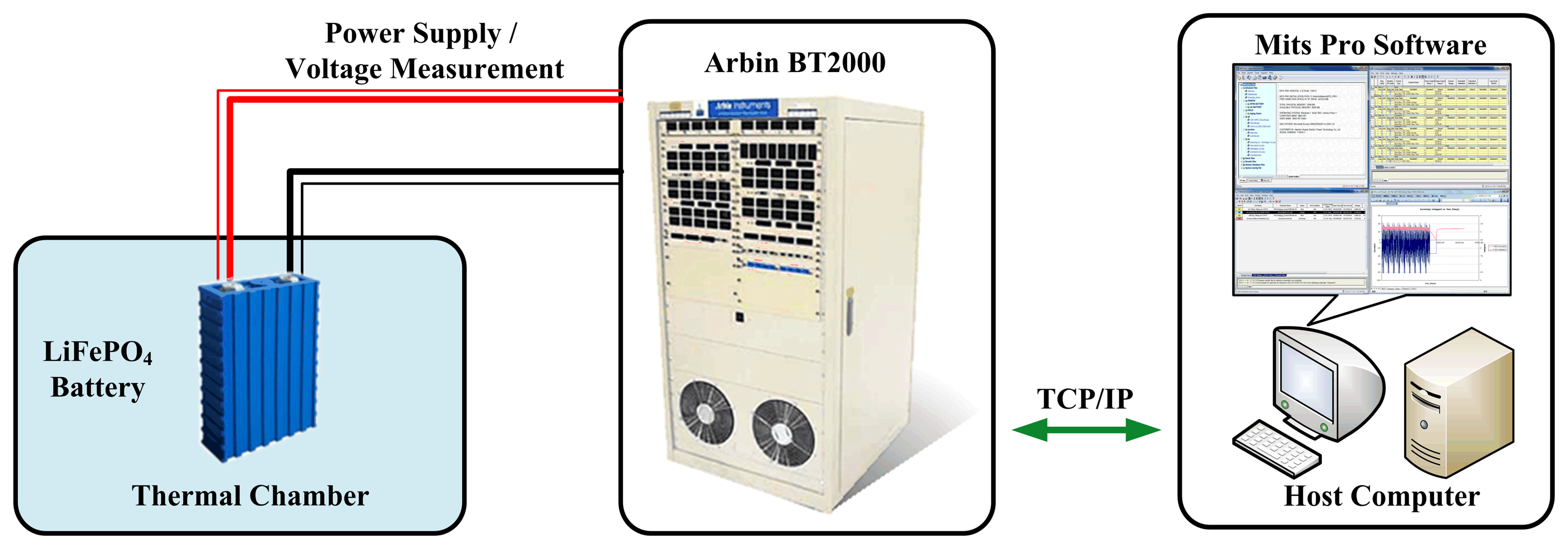
The test bench setup (Figure 1) consists of the following: (1) rectangular lithium-ion cells (LiFePO4, nominal voltage 3.3 V, nominal capacity 5 Ah, and upper/lower cut-off voltage 3.6/2.5 V.); (2) a thermal test chamber for environment, which has a temperature operation range between −55 and 150 °C; (3) a battery test system (Arbin BT2000 tester, Arbin, college town, TX, USA, which has a maximum voltage of 5 V and maximum charging/discharging current of ±200 A; the measurement inaccuracy of the current and voltage transducer inside the Arbin BT2000 system is within 0.1%); and (4) a PC with Arbins' Mits Pro Software for battery charging/discharging control. The Arbin BT2000 is connected to the battery cell placed inside the thermal chamber to maintain the temperature. The measured data are transmitted to the host computer through TCP/IP ports.
2.1.2. Available Capacity Test at Different Temperatures
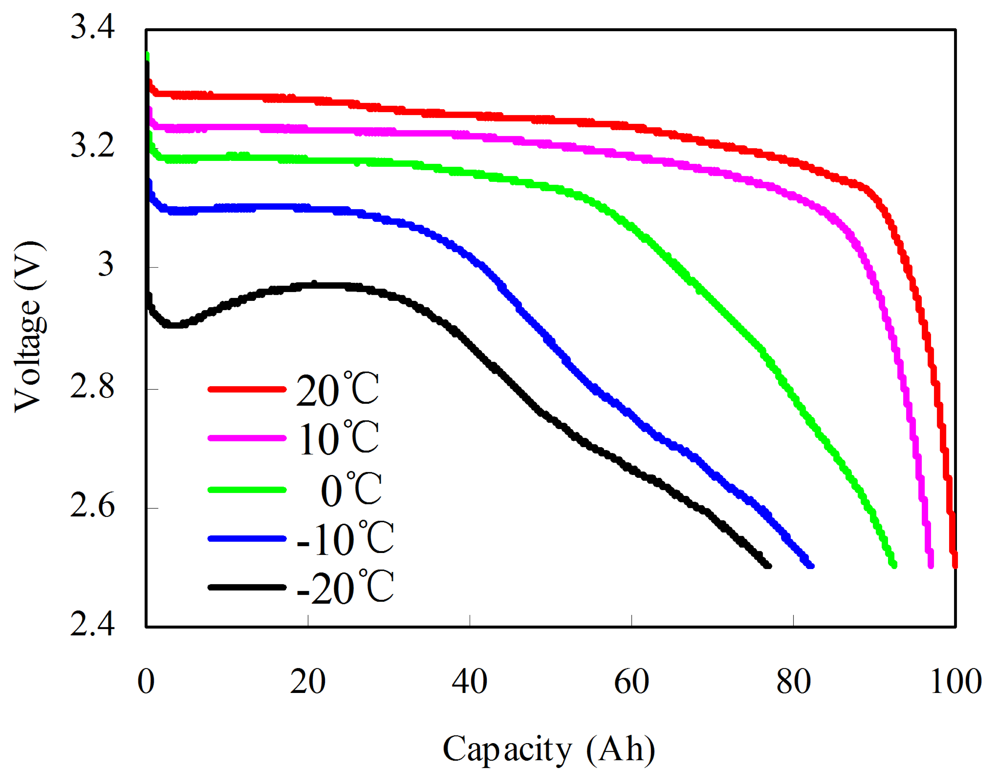
Given the temperature dependence of the capacity, the test is conducted from −20 to 20 °C at 10 °C intervals. The test procedures designed by many battery test manuals [33,34] at each temperature are as follows: (1) the cell is fully charged using a constant current of 1/3C rate until the voltage reaches to the upper cut-off voltage of 3.65 V at 20 °C; (2) the cell ambient temperature is decreased to the target temperature T; (3) a suitable soak period is employed for thermal equalization; and (4) the cell is fully discharged at a constant current of 1/3C rate until the voltage reaches the bottom cut-off voltage of 2.5 V. Figure 2 shows the discharge voltage curves at different temperatures. From −20 to 20 °C at an interval of 10 °C, the discharged capacities are 78, 84, 94, 98, and 100 Ah. In addition, the ohmic resistance R is most significantly increased as the temperature decreases. Thus, we may conclude that the poor performance of the lithium-ion batteries at low temperature originates from the substantially higher R, which can be further ascribed to the slow kinetics of the electrode reactions [32].
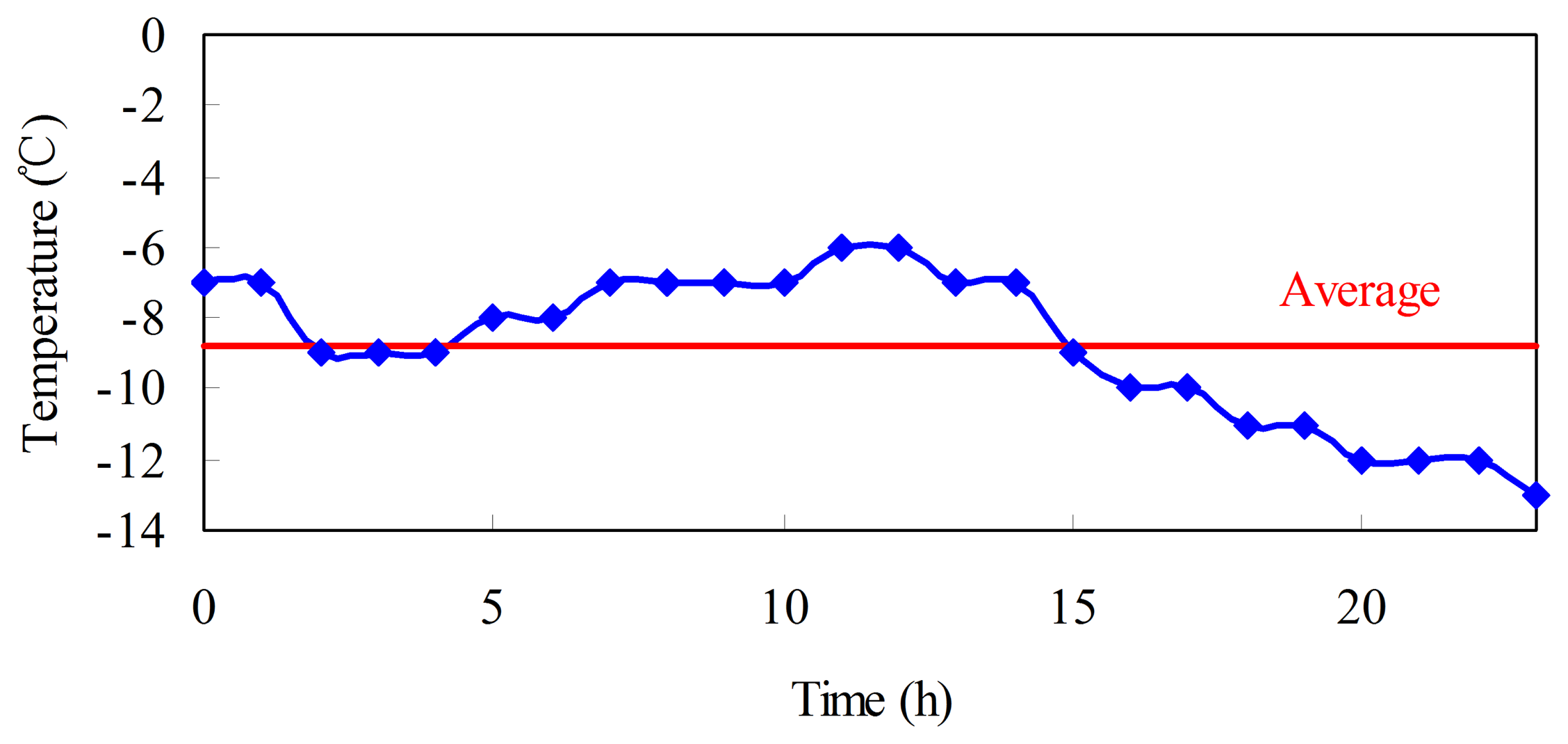
The purpose of the above test procedures is to verify the sustainable performance of capacities at different temperatures. Among these procedures, step (1) is implemented at room temperature, which is different from the ambient temperature in real vehicle applications. The operation temperature of the batteries without TMS in real vehicles varies along the ambient temperature. Figure 3 shows the temperature of Harbin in China during a regular day in winter [35]. The highest, lowest, and average temperatures that day are −6, −13, and −8.8 °C, respectively. Both charging and discharging processes in real vehicles occur at low temperature.
Therefore, the test procedures of available capacity at each temperature are redesigned as follows: (1) the cell ambient temperature is decreased to the target temperature T; (2) a suitable soak period is employed for thermal equalization; (3) the cell is fully charged using a constant current of 1/3C rate until the voltage reaches the upper cut-off voltage of 3.65 V at T, and then a 1 h rest is implemented; (4) finally, the cell is fully discharged at a constant current of 1/3C until the voltage reaches the bottom cut-off voltage of 2.5 V, wherein the available capacity of the cell is the number of ampere-hours that can be drawn from the battery. Steps 1 to 4 are repeated three times. If the error of the experimental results between the maximum and the average is within 2%, then the available capacity test is effective and the average value is considered as the available capacity; however, if the error is >2%, the available capacity test should be repeated. The results of available capacity at each temperature are shown in Table 1.
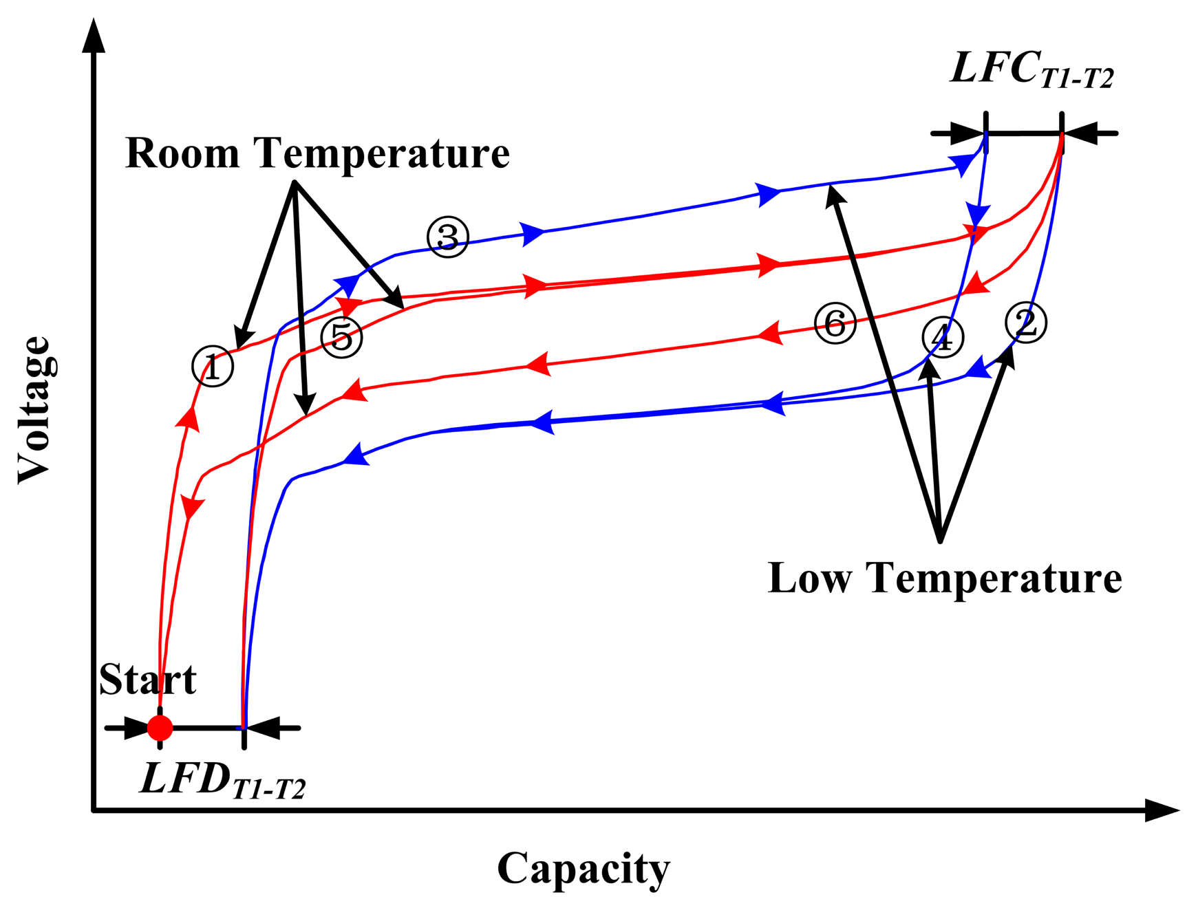
Although the battery is charged/discharged until the voltage reaches the same upper/bottom cut-off voltage at different ambient temperatures, the releasable capacity at each temperature varies. The capacity loss test is used to measure the difference of releasable capacities between two different temperatures. The difference between releasable capacities with fully charged battery at T1 and T2 is defined as the loss of full charge (LFCT1−T2). Likewise, the difference between releasable capacities with fully discharged battery at T1 and T2 is defined as the loss of full discharge (LFDT1−T2).
The test procedures of capacity loss at each temperature are as follows: (1) the cell is fully charged using a constant current of 1/3C until the voltage reaches the upper cut-off voltage of 3.65 V at T1; (2) the cell ambient temperature is decreased to T2, the cell is fully discharged at a constant current of 1/3C until the voltage reaches the bottom cut-off voltage of 2.5 V, and then the discharged capacity QChaT1−DisT2 is recorded; (3) the cell is fully charged using a constant current of 1/3C until the voltage reaches the upper cut-off voltage of 3.65 V; (4) the cell is fully discharged at a constant current of 1/3C until the voltage reaches the bottom cut-off voltage of 2.5 V and the charged capacity QChaT2−DisT2 is recorded; (5) the cell ambient temperature is then increased to T1, and the cell is fully charged using a constant current of 1/3C until the voltage reaches the upper cut-off voltage of 3.65 V; and (6) the cell is fully discharged at a constant rate of 1/3C until the voltage reaches the bottom cut-off voltage of 2.5 V and the discharged capacity QChaT1−DisT1 is recorded. The test process of capacity loss is shown in Figure 4. LFCT1−T2 is calculated as follows:
LFDT1−T2 is calculated as follows:
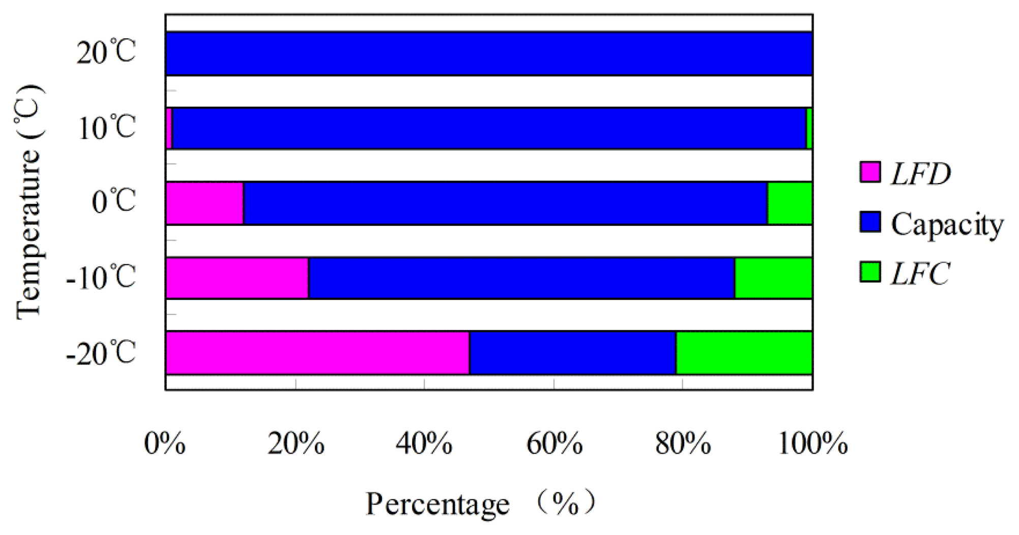
The results of LFD, LFC, and available capacity at each temperature with respect to the 20 °C 1/3C rate are presented in Table 2. The percentages of LFD, LFC, and available capacity at different temperatures are shown in Figure 5. Table 2 and Figure 5 show that LFD and LFC are different at the same temperature, in which LFD > LFC. Therefore, both the SOC definition and calculation at different temperatures should be redefined and recalibrated, corresponding to LFD, LFC, and available capacity.
2.2. Capacity with Different Currents
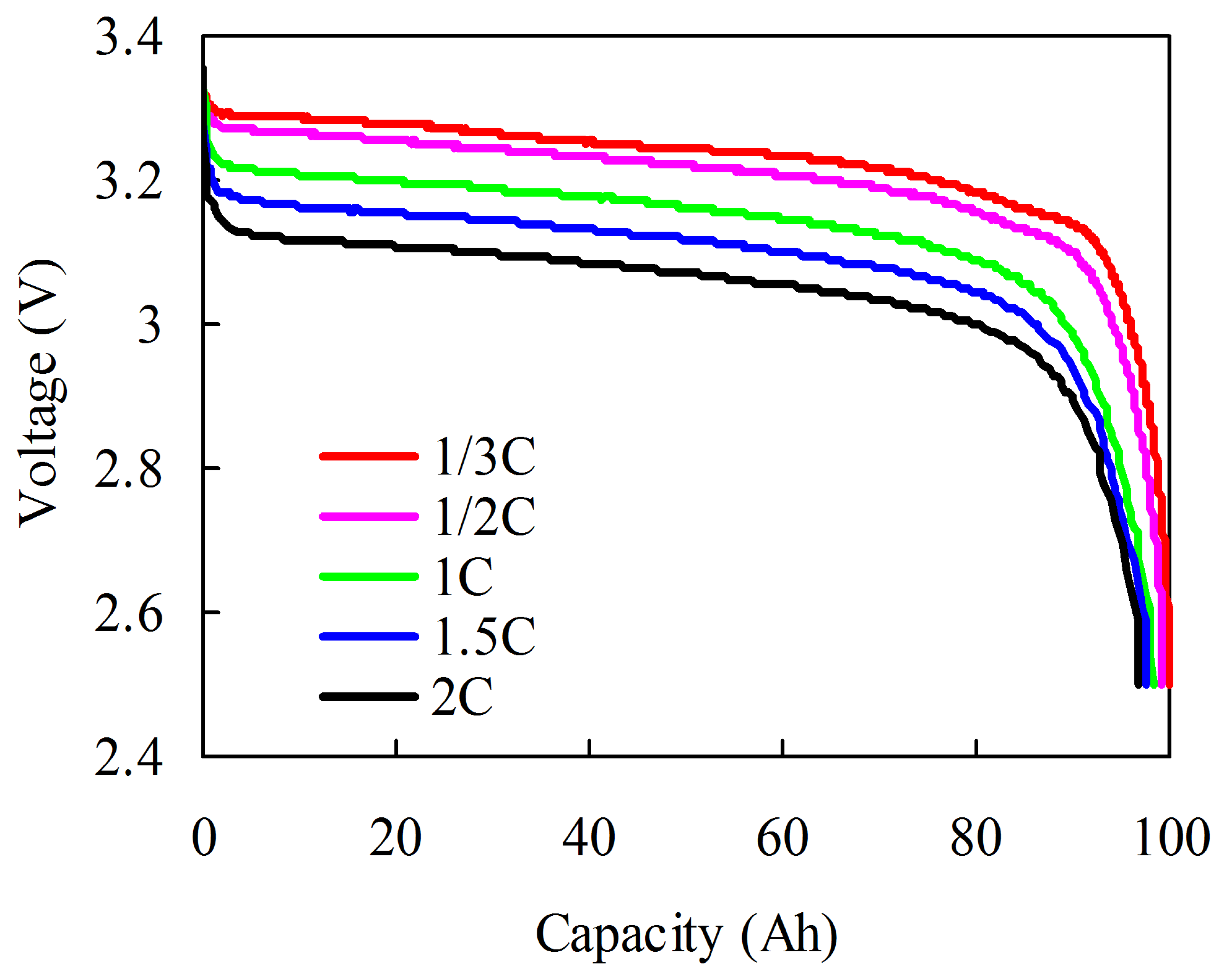
Current also influences capacity. A capacity test with different currents is conducted at C/3, C/2, 1C, 1.5C, and 2C rate. The capacities at C/3, C/2, 1C, 1.5C, and 2C (denoted as C3, C2, C, C2/3, and C1/2, respectively) are measured at the same temperature (20 °C). The test procedures at each rate are as follows: (1) the cell is fully charged using a constant current rate of C/3 until the voltage reaches the upper cut-off voltage of 3.65 V; (2) 1 h rest is implemented; (3) the cell is fully discharged at a constant current rate of C/3, C/2, 1C, 1.5C, or 2C until the voltage reaches the bottom cut-off voltage of 2.5 V; and (4) then another rest for 1 h. Figure 6 shows the discharge curves at different current rates. Less than 3% of the C1/2 capacity is not accessible with respect to the C3 capacity.
Compared with the temperature effect, the influence of current on capacity is relatively small. Moreover, in real vehicle applications, the battery pack is charged with a suitable current, as recommended by the manufacturer. Although a sophisticated dynamic current profile is run on the battery pack when the vehicle is working, the large current is limited by BMS within a reasonable range. To satisfy the requirement of power and energy for xEVs, a suitable battery pack size is selected during the design phase. Thus, the battery pack is mainly operated in the high-efficiency area and the large current does not last for a long time. In addition, the influence of current on capacity is temporarily neglected in SOC estimation.
3. Coulombic Efficiency
Coulombic efficiency is another important parameter of SOC estimation. Battery coulombic efficiency, like capacity, is sensitive to current and temperature. Therefore, current and temperature must also be specified in the definition of coulombic efficiency. In the last section, capacity losses at different currents and temperatures mainly involve changes in the thermodynamic and in the kinetic aspects of a battery [4]. Unlike the capacity loss, the coulombic efficiency is mainly caused by the energy loss that occurs during charging and discharging.
3.1. Definition of Coulombic Efficiency
Coulombic efficiency is the ratio of the Ah removed from a battery during discharging to the Ah required to restore the battery to the SOC before discharging [33]. The coulombic efficiency is defined as:
Qcharge is not equal to Qdischarge, which is primarily caused by the energy loss along with the charging/discharging process. The energy loss leads to the variation in charging/discharging time, which results in the variation in charging/discharging capacity. The energy loss during charging/discharging is mostly thermal loss. The thermal generation factors are decomposed into three elements, namely, reaction heat value, polarization heat value, and Joule heat value, which vary according to the variations in current and temperature [36].
Energy loss also depends on current and temperature. Therefore, the same number of charge that enters/exits the battery during charging/discharging at different currents and temperatures need different amounts of energy. The equivalent charge/discharge coulombic efficiency is defined as the ratio of the charged/discharged capacity at the non-rated condition to the charged/discharged capacity at the rated condition. The equivalent charge coulombic efficiency is given as:
The equivalent discharge coulombic efficiency is given as:
3.2. Calculation of Coulombic Efficiency
According to the different currents and temperatures running Qcharge and Qdischarge for various possible configurations, 16 kinds of coulombic efficiency can be obtained (Table 3). In Table 3, the charge capacities at different conditions are in the first row and the discharge capacities at different conditions are in the first line. The coulombic efficiencies at different conditions are in the cross location.
For example, the charge capacity at rated condition is on the first row and the discharge capacity at rated condition is on the first line. Consequently, the cross location of the first row and the first line is the rated coulombic efficiency , which can be measured through the following test procedures: (1) the battery is discharged using IR rate at TR until bottom cut-off voltage is reached; (2) the battery is rested for 1 h until it returns to the equilibrium state; (3) the battery is charged using IR rate at TR until upper cut-off voltage is reached, and the charge capacity is ; (4) the battery is rested for 1 h until it returns to the equilibrium state; (5) the battery is discharged using IR rate at TR until bottom cut-off voltage is reached, and the discharged capacity is . The calculation method of other coulombic efficiencies in Table 3 is similar to that of the rated coulombic efficiency.
According to the definition of equivalent charge/discharge coulombic efficiency, we can extend it to a more comprehensive equivalent charge/discharge coulombic efficiency, which is not only between non-rated condition and rated condition but also between different conditions. According to the different currents and temperatures running Qcharge and Qdischarge for various possible configurations, 10 kinds of equivalent charge/discharge coulombic efficiencies can be obtained (Tables 5 and 6). In these two tables, the standard charge/discharge capacity (denominator in equivalent charge/discharge coulombic efficiencies) is on the first row and the non-standard charge/discharge capacity (numerator in equivalent charge/discharge coulombic efficiencies) is on the first line. Correspondingly, the equivalent charge/discharge coulombic efficiencies between different conditions are in the cross location.
For example, the charge capacity at non-rated condition is on the first row and the charge capacity at rated condition is on the first line. Consequently, the cross location of first row and first line is the rated equivalent charge coulombic efficiency . The equivalent charge/discharge coulombic efficiency cannot be directly measured through experiment. Therefore, we transform as follows:
3.3. Influence of Current and Temperature on Coulombic Efficiency
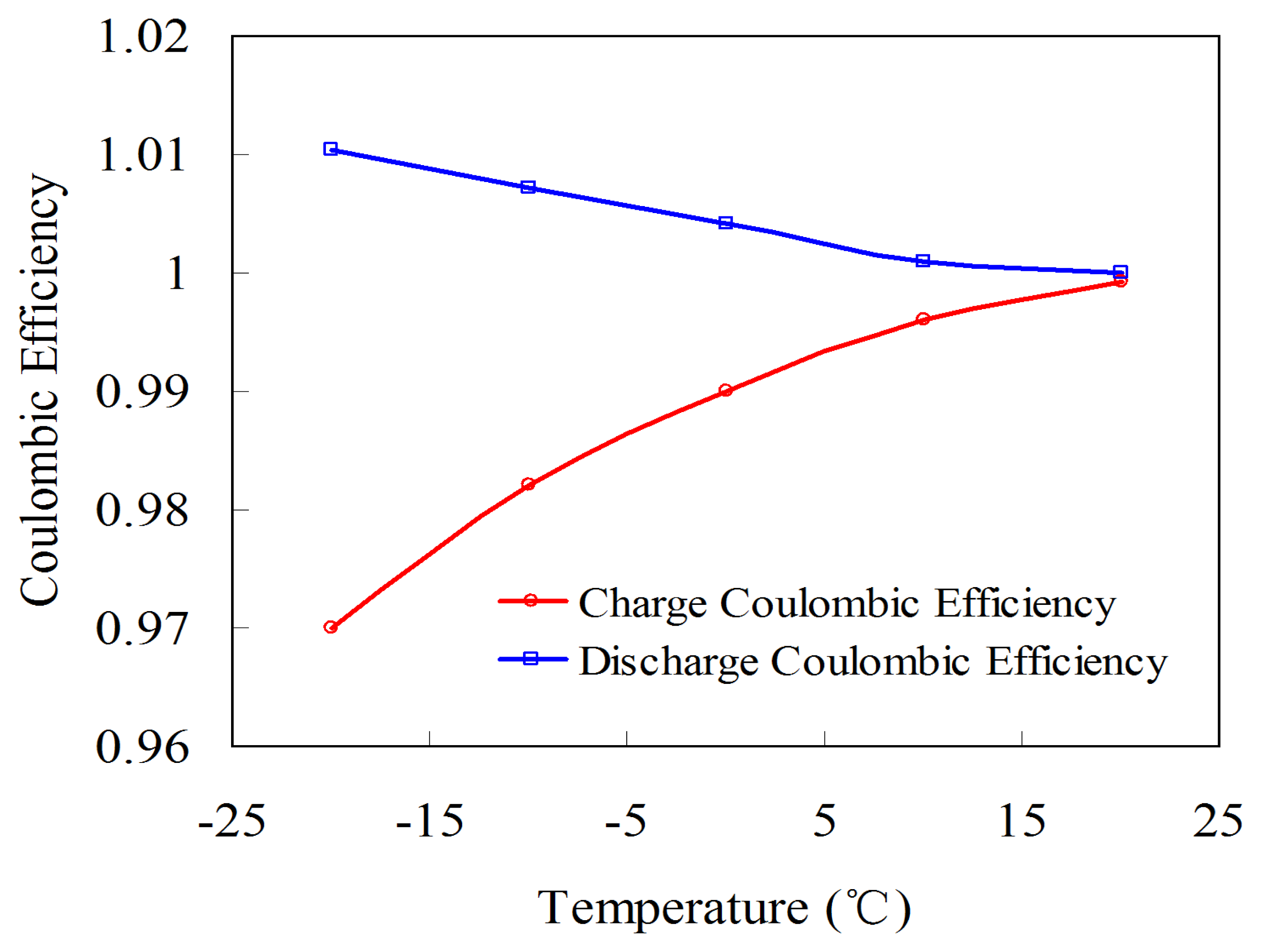
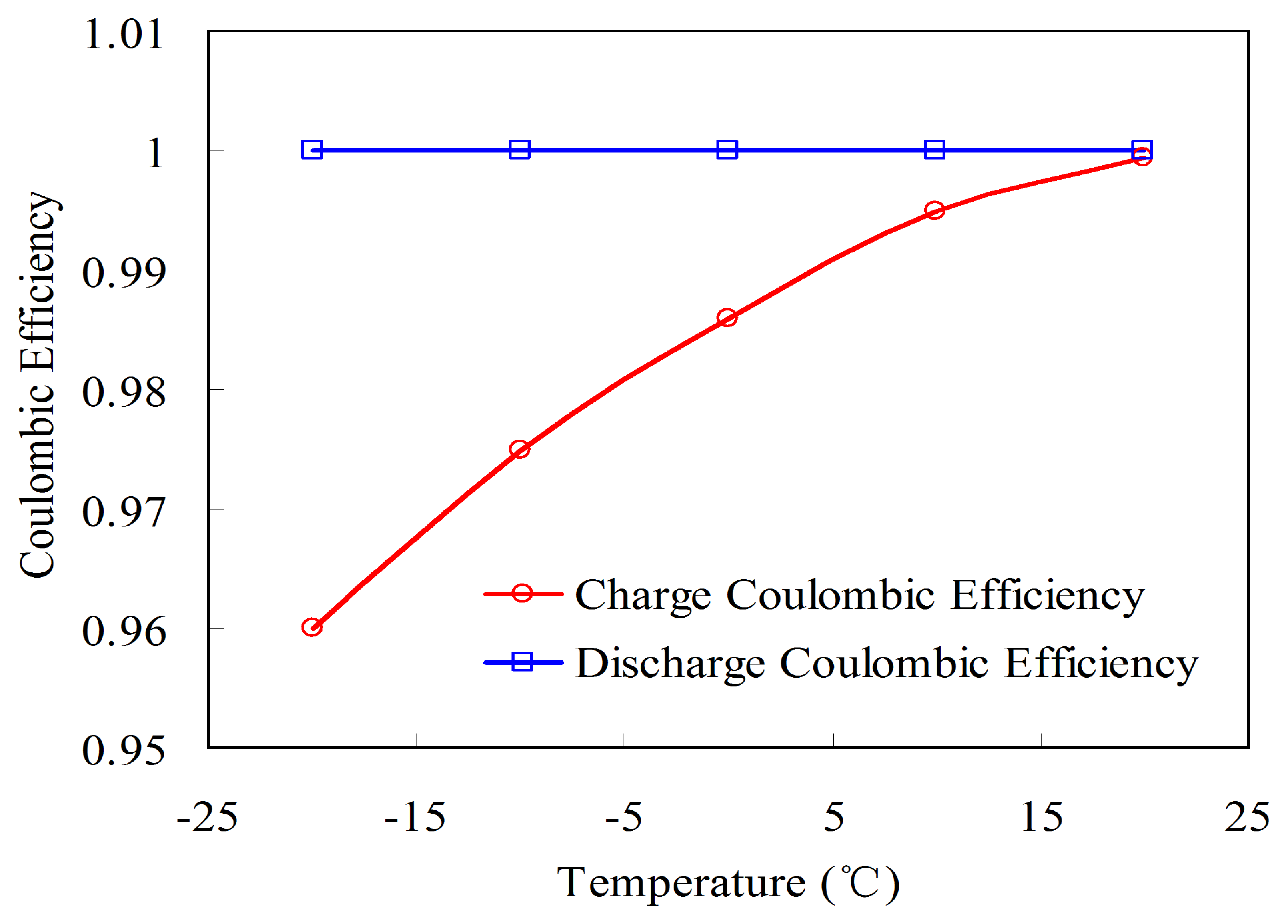
Figure 7 shows the influence of current (C/3, C/2, 1C, 1.5C, and 2C) and temperature (20, 10, 0, −10, and −20 °C) on coulombic efficiency. Figure 7 shows that the current has subtle effects on coulombic efficiency. At 20 °C, the coulombic efficiency at C/3 and 2C is 0.999 and 0.998, respectively. In real vehicle applications, although the loading current is a sophisticated dynamic profile, the duration of the large current is short. Therefore, the influence of the current on the coulombic efficiency is ignored in later sections. However, temperature has more significant effects on coulombic efficiency than current (Figure 6). Under C/3 rate, the coulombic efficiency at 20 and −20 °C are 0.999 and 0.96, respectively. Therefore, the influence of temperature on coulombic efficiency should be considered for the SOC estimation.
4. SOC Estimation
On the basis of the analysis in Section 2, the available capacity is influenced by current and temperature. Therefore, with regard to the variation in available capacity, SOC should be redefined. In this section, we provide the definition of the rated/non-rated SOC according to the available capacity at the rated and non-rated condition. The calculation of the rated/non-rated SOC is then developed to meet the applications at different conditions.
4.1. Definition of SOC
4.1.1. Definition of the Rated SOC
The rated capacity CIR,TR is the capacity when the fully charged battery is completely discharged at the rated condition. The rated releasable capacity is the releasable capacity when the operating battery is completely discharged at the rated condition. Accordingly, the rated SOC is defined as the percentage of the rated releasable capacity relative to the rated capacity:
The rated SOC is based on the rated capacity that is unaffected by current and temperature. On the basis of the analysis in Section 2, the influence of current on available capacity is neglected. Therefore, the rated SOC is applied to the batteries with TMS, which can maintain the temperature of batteries in the rated temperature range.
4.1.2. Definition of the Non-Rated SOC
The non-rated capacity CI,T is the capacity when the fully charged battery is completely discharged at non-rated condition. By contrast, the non-rated releasable capacity is the releasable capacity when the operating battery is completely discharged at the non-rated condition. The non-rated SOC is a relative quantity that describes the ratio of the non-rated releasable capacity to the non-rated capacity of the battery. The non-rated SOC is given as:
Compared with the rated SOC, the non-rated SOC is based on the non-rated capacity influenced by current and temperature. Therefore, the non-rated SOC is applied to the batteries without TMS. In this case, the temperature of batteries changes with the ambient temperature.
4.2. Calculation of Advanced Ah Counting Method
4.2.1. Calculation of the Rated SOC
The rated SOC is based on the rated capacity CIR,TR. However, real vehicle tests show a sophisticated dynamic current profile with different charge and discharge currents. Therefore, the charged and discharged capacity at different conditions should be converted into the discharged capacity at rated condition. In the charging process, we use the coulombic efficiency to convert the non-rated charged capacity into the rated discharged capacity. In the discharging process, the equivalent coulombic efficiency is used to convert the different conditions of discharge capacity into the rated discharged capacity. With a measured charging/discharging current I and the corresponding coulombic efficiency, the rated SOC in an operating period Δt can be calculated using Equation (9):
When the rated SOC is calculated using Equation (9), the coulombic efficiency ηIR,TR is as follows:
On the basis of the analysis in Section 3.4, the influence of current on coulombic efficiency is neglected. Therefore, the calculation of coulombic efficiency ηIR,TR is based on the rated current IR, and the coulombic efficiency ηIR,TR is as follows:
4.2.2. Calculation of the Non-Rated SOC
Compared with the rated SOC, the non-rated SOC is based on the non-rated capacity CI,T. Therefore, the charged and discharged capacities at different conditions should be converted into the discharged capacity at the battery operating condition. In the charging process, we use the coulombic efficiency to convert the charged capacity under different conditions into the discharged capacity under the corresponding condition. In the discharging process, given that the discharged capacity is under the current operating condition, the equivalent coulombic efficiency is .With a measured charging/discharging current I and the corresponding coulombic efficiency, the non-rated SOC in an operating period Δt can be calculated using:
When the non-rated SOC is calculated using Equation (12), the coulombic efficiency ηI,T is as follows:
On the basis of the analysis in Section 2.2, the influence of current on capacity is negligible. Therefore, the non-rated SOC is based on CIR,T in real vehicle application. Based on Section 3.4, the influence of current on coulombic efficiency is also negligible. In addition, the calculation of coulombic efficiency ηI,T is based on the rated current IR. The coulombic efficiency ηI,T is as follows:
In addition to the influence of temperature on coulombic efficiency, the variation in available capacity at different temperatures should be considered in calculating the non-rated SOC. Although the battery has the same releasable capacities, SOCs are different at different temperatures. Therefore, SOCs between different temperatures should be converted depending on the available capacity and capacity loss. According to Equation (12), SOCI,T(t) is the current temperature SOC, whereas SOCI,T(t − 1) is the SOC converted from the last temperature to the current temperature. The conversion procedure of SOC between different temperatures is as follows:
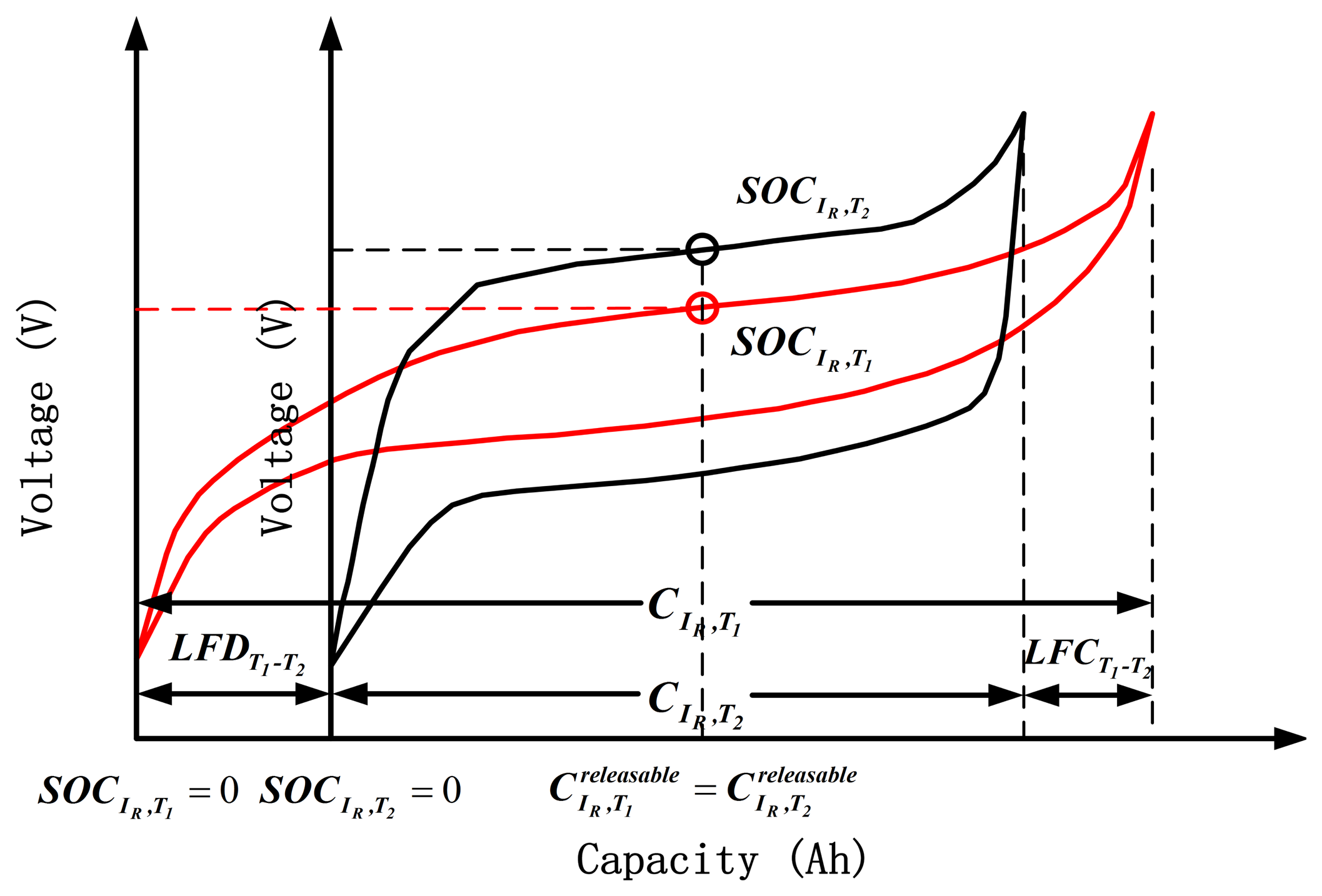
The battery soaked in the temperature of T1 and T2 (supposing T1 > T2) has the same releasable capacities (Figure 10). At the two temperatures, the corresponding SOCs are SOCIR,T1 and SOCIR,T2, and the available capacities are SOCIR,T1 and SOCIR,T2, respectively. The LFD between these two temperatures is LFDT1−T2. At temperature T1, the releasable capacity is:
At temperature T2, the releasable capacity is:
Given that the releasable capacities are the same at T1 and T2, i.e., , then:
When the battery is cooled from T1 to T2, SOCIR,T1 is converted into SOCIR,T2 as follows:
When the battery is warmed from T2 to T1, SOCIR,T2 is converted into SOCIR,T1 as follows:
5. Initial SOC Estimation by Multistate OCV
SOC is related to the embedding quantity of lithium-ion in the active material and with static thermodynamics. Therefore, the OCV after adequate resting can be considered to reach balanced potential because one-to-one correspondence exists between OCV and SOC and bear little relation to the service life of batteries; it is also an effective method to estimate SOC of lithium-ion batteries [21,37]. The initial SOC in Ah counting method can be revised using the OCV method.
Corresponding to the rated/non-rated SOC in the last section, the rated/non-rated OCV–SOCs are established to estimate the initial SOC. To estimate the non-rated initial SOC under different temperature paths, we further establish the R–L non-rated OCV–SOCs and the L–L non-rated OCV–SOCs. SOC estimation by the above OCV–SOCs at different conditions is defined as multistate OCV method.
5.1. Rated OCV–SOCs
The rated OCV–SOCs are established to estimate the rated initial SOC. The relationship between SOC and OCV should be based on the rated capacity SOCIR,TR, which guarantees that SOCs estimated by Ah counting method (SOCAh) and OCV method (SOCOCV) have good consistency.
The rated SOC is generally applied to batteries with TMS. Although TMS exist in battery packs, vehicles also experience cold cranking in winter. In the cold cranking process, the TMS cannot warm the battery on time, which causes a low internal temperature of the battery. Given the OCV thermosensitivity, gaps exist in the OCV–SOCs at different temperatures. In addition, OCV exhibits pronounced hysteresis phenomena, resulting in the non-overlapped charged and discharged OCV–SOC [30]. In the current paper, we only introduce the charged OCV test procedures, and the discharged test is the inverse process of the charged test.
The rated OCV–SOC test procedures are as follows: (1) the cell is fully discharged using a constant current of 1/3C rate until the voltage reaches the cut-off voltage of 2.5 V at 20 °C; (2) After a suitable period of rest (generally more than 3 h), the measured OCV is at SOC = 0%, which is denoted as OCVrated(SOCIR,TR = 0, T=20). The cell is then soaked at 10 °C for a suitable period, and the measured OCV is OCVrated(SOCIR,TR = 0, T=10). The OCV measurement is conducted from −20 °C to 20 °C at an interval of 10 °C. After the OCV measurement, the cell is again soaked at 20 °C for a suitable period; (3) the cell is then charged at a constant current of C/3 rate until the charged Ah reaches CIR,TR/20, which corresponds to SOCIR,TR = 5. With the same process in step (2), the OCVs are measured from OCVrated(SOCIR,TR = 5, T=20) to OCVrated(SOCIR,TR = 5, T=−20). Steps (2) and (3) are repeatedly performed until SOC = 0% to 100% at an interval of 5% has been achieved.
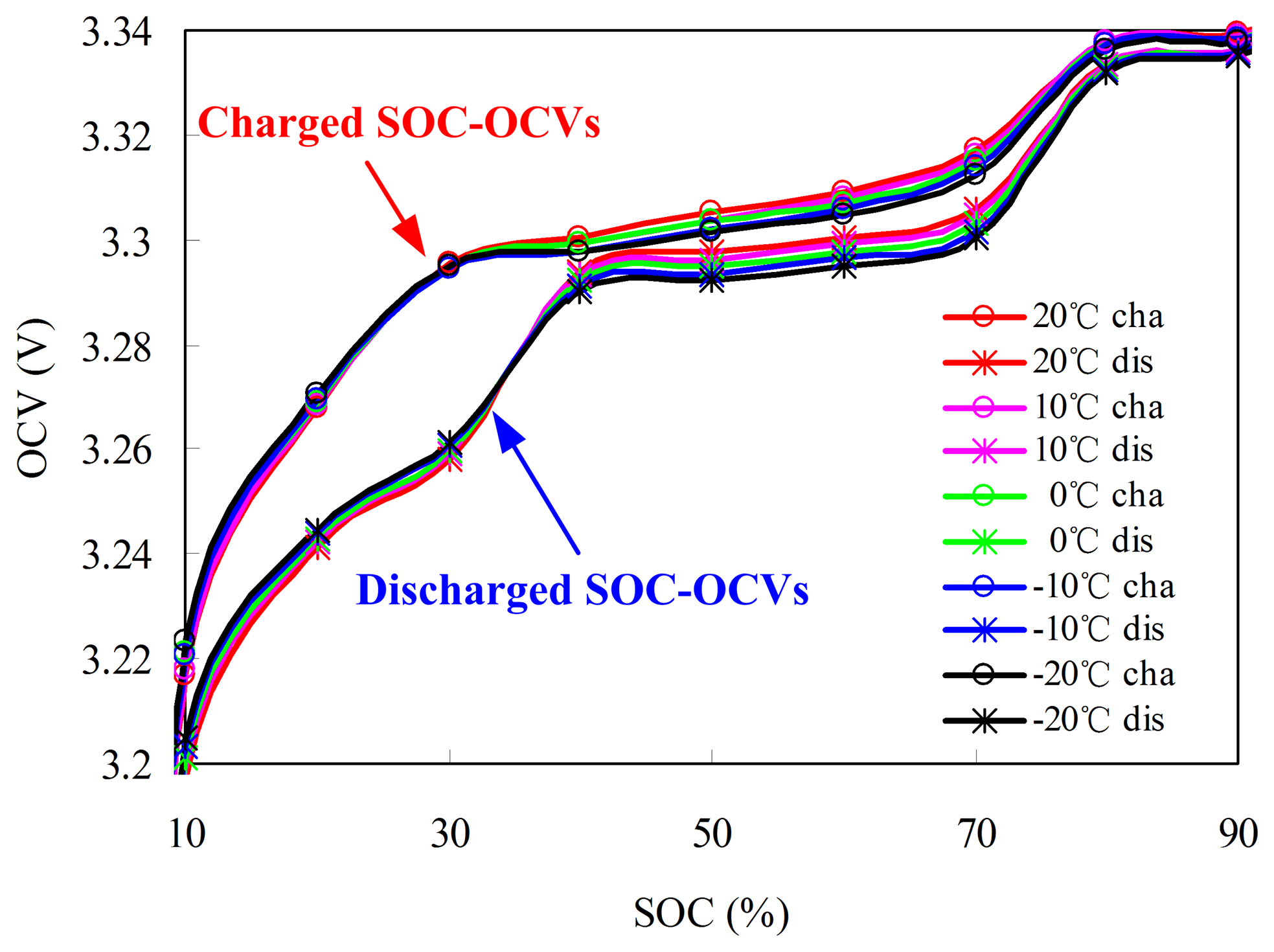
Five charged and discharged OCV–SOCs are obtained from −20 °C to 20 °C at an interval of 10 °C. Figure 11 emphasizes the charged and discharged OCV–SOCs between 10% and 90% SOC at different temperatures. The OCVs at the same SOC have lower temperature. The rated OCV–SOC at T1 is described using:
The rated OCV–SOCs can be obtained using the rated OCV–SOC at different temperatures with the fitting method:
As shown in Figure 10, the charged OCV–SOCs are higher than the discharged OCV–SOCs, indicating that hysteresis phenomenon of the OCV occurs during charging/discharging. The SOC based on the charged OCV–SOC is smaller than that based on the discharged OCV–SOC at the same temperature. Therefore, the effect of the hysteresis should not be ignored. If the battery is charged before rest, then the charged OCV–SOCs are used to estimate the initial SOC; otherwise, the discharged OCV–SOCs are used. In the later sections, we deal with the OCV hysteresis in the same way.
5.2. Non-Rated OCV–SOCs
Compared with the rated OCV–SOCs, the non-rated OCV–SOCs are established to estimate the non-rated initial SOC. The non-rated SOC is based on CI,T, which is significantly influenced by temperature. To ensure SOC consistency between SOCAh and SOCOCV, the effects of temperature on the available capacity and capacity loss should be considered in establishing the non-rated OCV–SOCs.
The non-rated SOC is generally applied to the batteries without TMS. In real vehicle applications, the battery pack without TMS experiences the following two cases of temperature variation: (1) the vehicle works at room temperature during daytime and rests in the evening. Given the large temperature difference during the day, the temperature sharply decreases in the evening. The next morning, the vehicle is restarted at low temperature; (2) The vehicle is operated at low temperature all the time. We define the above two cases as the different temperature paths: (1) From room temperature to low temperature (R–L) and (2) from low temperature to low temperature (L–L).
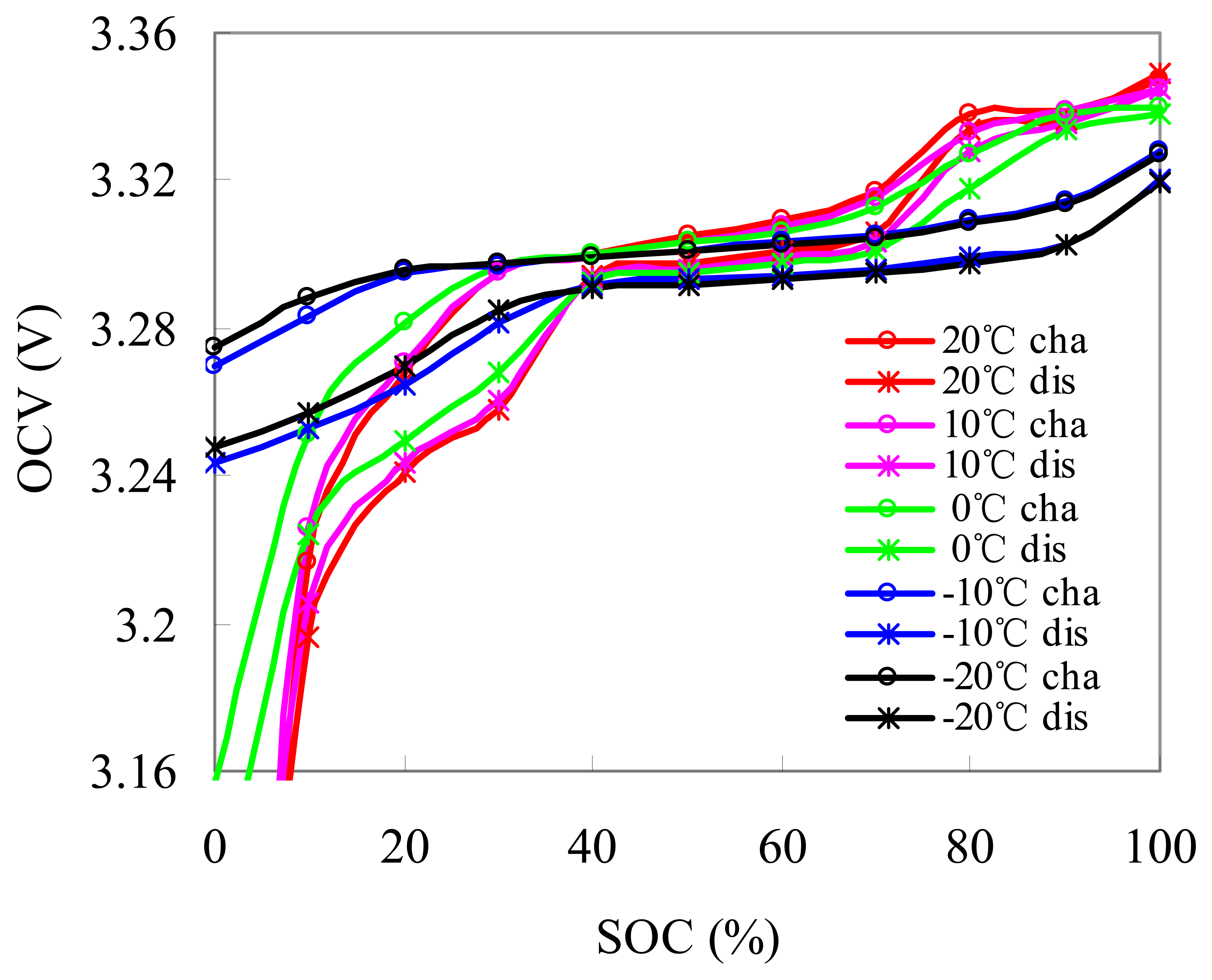
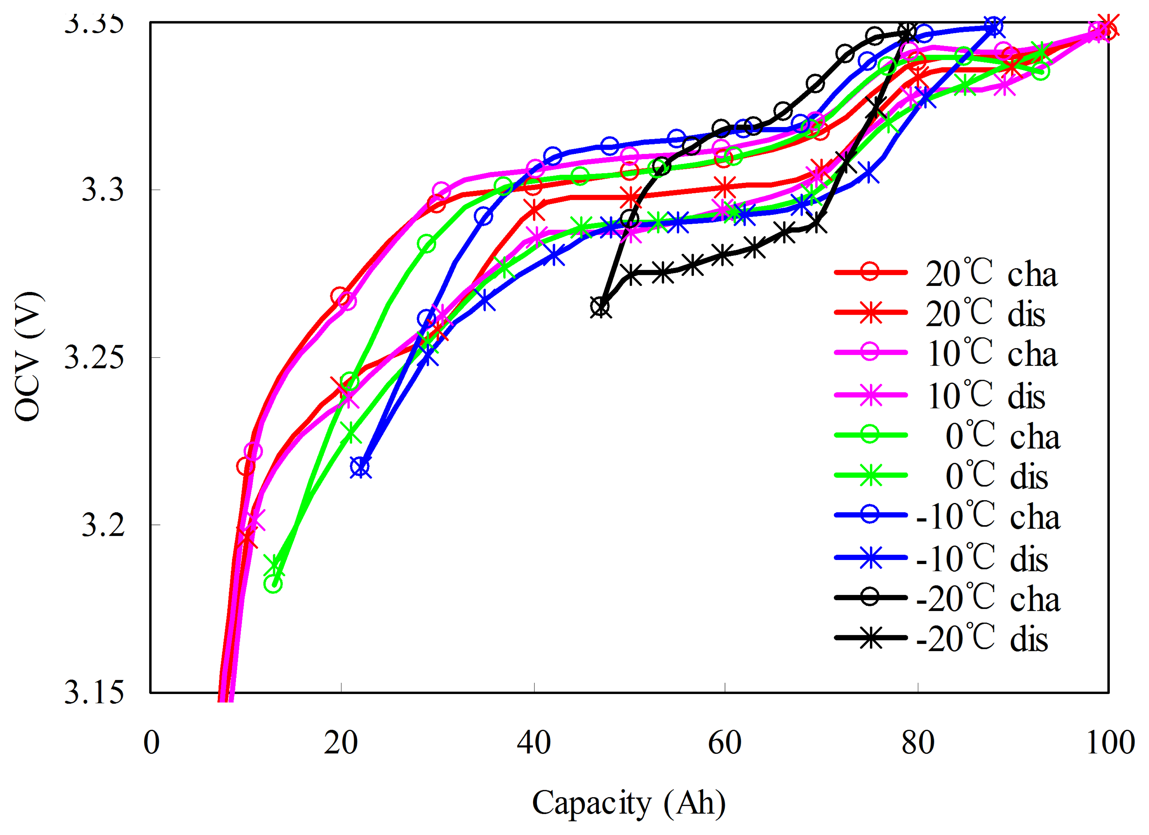
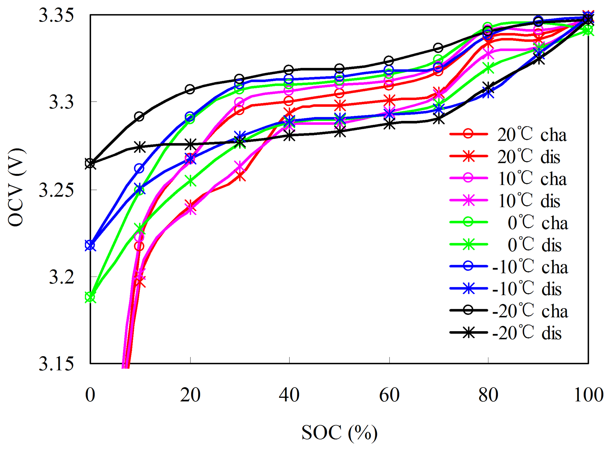
OCV is affected by the different temperature paths that cause errors in SOC estimation. Figure 11 shows the OCV–SOCs at 0 °C in different temperature paths. The R–L charged and discharged OCV–SOCs are measured as 4.2.1 test procedures. However, the L–L charged and discharged OCV–SOCs are measured as follows: (1) the cell is fully discharged using a constant current of 1/3C rate until the voltage reaches the cut-off voltage of 2.5 V at 20 °C; (2) the cell ambient temperature is decreased to the target temperature 0 °C and a suitable soak period is implemented for thermal equalization; (3) the cell is then charged at a constant current of C/3 rate until the Ah reaches CIR,TR/20. A suitable period is implemented until it returns to the equilibrium state. Step (3) is repeatedly performed until the battery reaches the upper cut-off voltage of 3.65 V. The voltages during each rest period are recorded to establish the L–L OCV–SOCs.
As shown in Figure 12, the OCV–SOCs in different temperature paths are different even at the same temperature. The charge/discharge OCVs decrease/increase with the increase in ambient temperature, and this phenomenon results from the entropy change [38]. To estimate the initial SOC in different temperature paths, we establish the R–L non-rated OCV–SOCs and the L–L non-rated OCV–SOCs, respectively.
5.2.1. R–L Non-Rated OCV–SOCs
The R–L non-rated OCV–SOCs are converted using the rated OCV–SOCs according to the available capacity and capacity loss at different temperatures. Considering the rated OCV–SOC at T1 as an example to demonstrate the process, the detailed procedures are in Figure 13. We assume that the rated OCV–SOC at TR and T1 are known as OCVrated(SOCIR,TR ,TR) and OCVrated(SOCIR,TR ,T1), respectively. According to the available capacity and capacity loss at T1 (CIR,T1,,LFDTR−T1, and LFCTR−T1), the domain of SOCIR,TR in OCVrated(SOCIR,TR,T1) is [LFDTR−T1/CIR,TR, (LFDTR−T1 + CIR,T1)/CIR,TR], as shown in Figure 13a. By OCV(SOCIR,TR ,T1) horizontal translation LFDTR−T1/CIR,TR and horizontal scaling CIR,T1/CIR,TR, the domain of SOCIR,TR is converted into [0,100]. The function of OCVrated(SOCIR,TR,T1) is transformed into OCVrated((CIR,T1SOCIR,TR + LFDTR−T1)/CIR,TR,T1) as shown in Figure 13b.
Figure 14 shows the charged and discharged R–L non-rated OCV–SOCs. The R–L non-rated OCV–SOC at T1 is described by:
The R–L non-rated OCV–SOCs can be obtained using the R–L non-rated OCV–SOC at different temperatures with the use of the fitting method:
5.2.2. L–L Non-Rated OCV–SOCs
Considering T1 as an example, the L–L non-rated OCV–SOC test procedures at each temperature are as follows: (1) the cell is soaked in the target temperature T1 for a suitable period for thermal equalization, and then fully discharged using a constant current of 1/3C rate until the voltage reaches the cut-off voltage of 2.5 V; (2) after a suitable period of rest, the measured OCV is at SOC = 0%, which is denoted as OCVL−L(SOCIR,TR = 0); (3) the cell is then charged at a constant current of C/3 rate until Ah reaches CIR,T1/20 Ah, which corresponds to SOCIR,T1 = 5. After a suitable period of rest, the measured OCV is at SOCIR,T1 = 5, which is denoted as OCVL−L(SOCIR,T1 = 5). Step (3) is repeatedly performed until SOC = 0% to 100% at an interval of 5% is achieved.
Figure 15 shows the charged and discharged L–L non-rated OCV–SOCs with respect to the capacity. The start and end points on X axis of OCV–SOC at different temperatures correspond to LFDTR−T and LFDTR−T1 + CIR,T, which guarantee that the SOCOCV estimated by L–L non-rated OCV–SOCs and SOCAh are consistent. Figure 16 shows the charged and discharged L–L non-rated OCV–SOCs with respect to SOC. The L–L non-rated OCV–SOC at T1 is described by:
The L–L non-rated OCV–SOCs can be obtained using the L–L non-rated OCV–SOC at different temperatures with the fitting method:
6. Experimental Results for SOC Estimation
According to whether the battery pack is with/without TMS, we calculate the rated SOC/non-rated SOC, respectively. The calculation procedures of the rated SOC are as follows. When the vehicle is started, the BMS measures the temperature of the battery pack. According to the measured temperature, we propose the application of the rated OCV–SOCs instead of the conventional OCV–SOC, which is often established at room temperature, to estimate the rated initial SOC. The other parameters in the rated SOC algorithm, such as ηIR,TR and CIR,TR, can be determined according to the rated condition. For the non-rated SOC, the battery pack temperature is also measured and saved in the BMS. By comparing the current temperature and the previous temperature stored in the memory of BMS, we could obtain the temperature path. According to the temperature path R–L or L–L, the corresponding non-rated OCV–SOCs are selected to estimate the non-rated initial SOC. In the process of calculation, SOCI,T(t) is the SOC at current temperature, whereas SOCI,T(t − 1) is the SOC converted from the last temperature to the current temperature. Meanwhile, the other parameters in the non-rated SOC algorithm, such as ηI,T and CI,T, are employed according to the measured ambient temperature. A flow chart based on the developed method is shown in Figure 17.
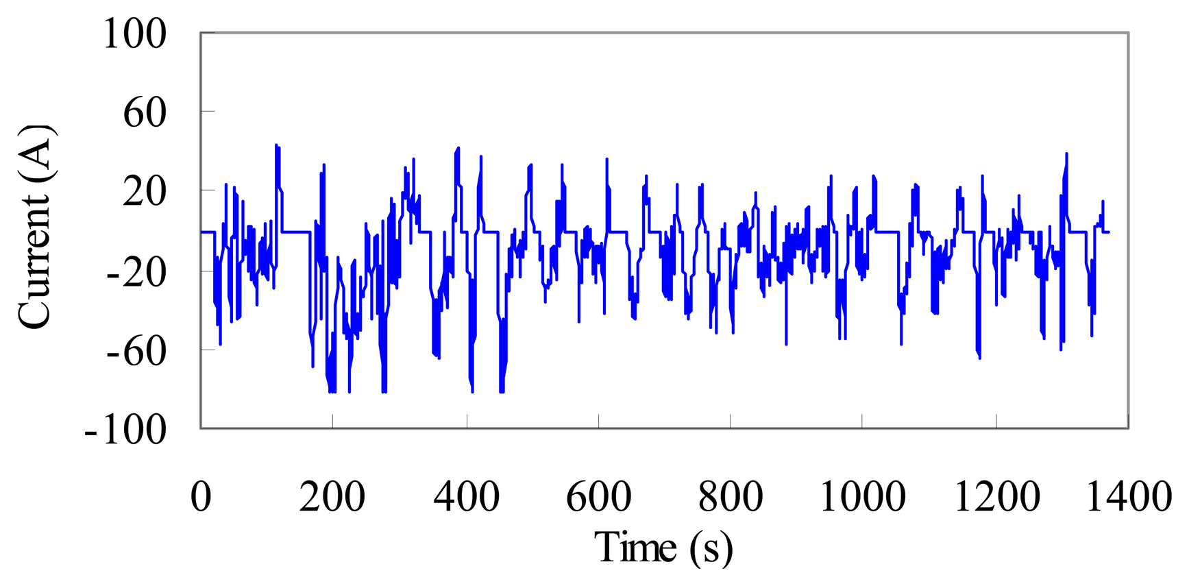
A validation test with a sophisticated dynamic current profile, the federal urban driving schedule (FUDS) is conducted to verify the SOC estimation algorithm. In the laboratory test, a dynamic current sequence is transferred from the FUDS time–velocity profile. The current sequence is then scaled to fit the specification of the test battery. A completed FUDS current profile over 1372 s is emphasized in Figure 18. FUDS tests are conducted at different ambient temperatures to emulate the operation conditions. The validation tests are separately implemented under constant and alternated temperatures.
6.1. Constant Temperature Test
The constant temperature test is used to validate the performance of the SOC by Ah counting (SOCAh) and initial SOC (SOCOCV) estimation at different constant temperatures. The test is conducted at −10, 0, and 20 °C. The other temperature tests are similar.
The pre-test is conducted before the constant temperature test. The cell is charged using the constant current of C/3 rate at TR until Ah reaches 0.7CIR,TR Ah. The cell is then soaked at target temperature T for a suitable period. The test procedures of constant temperature test at each target temperature (−10, 0, and 20 °C) are as follows: (1) pre-test; (2) nine FUDS cycles are loaded to the cell, followed by 12 h rest; (3) the cell is discharged using the constant current of C/3 rate until bottom cut-off voltage is reached.
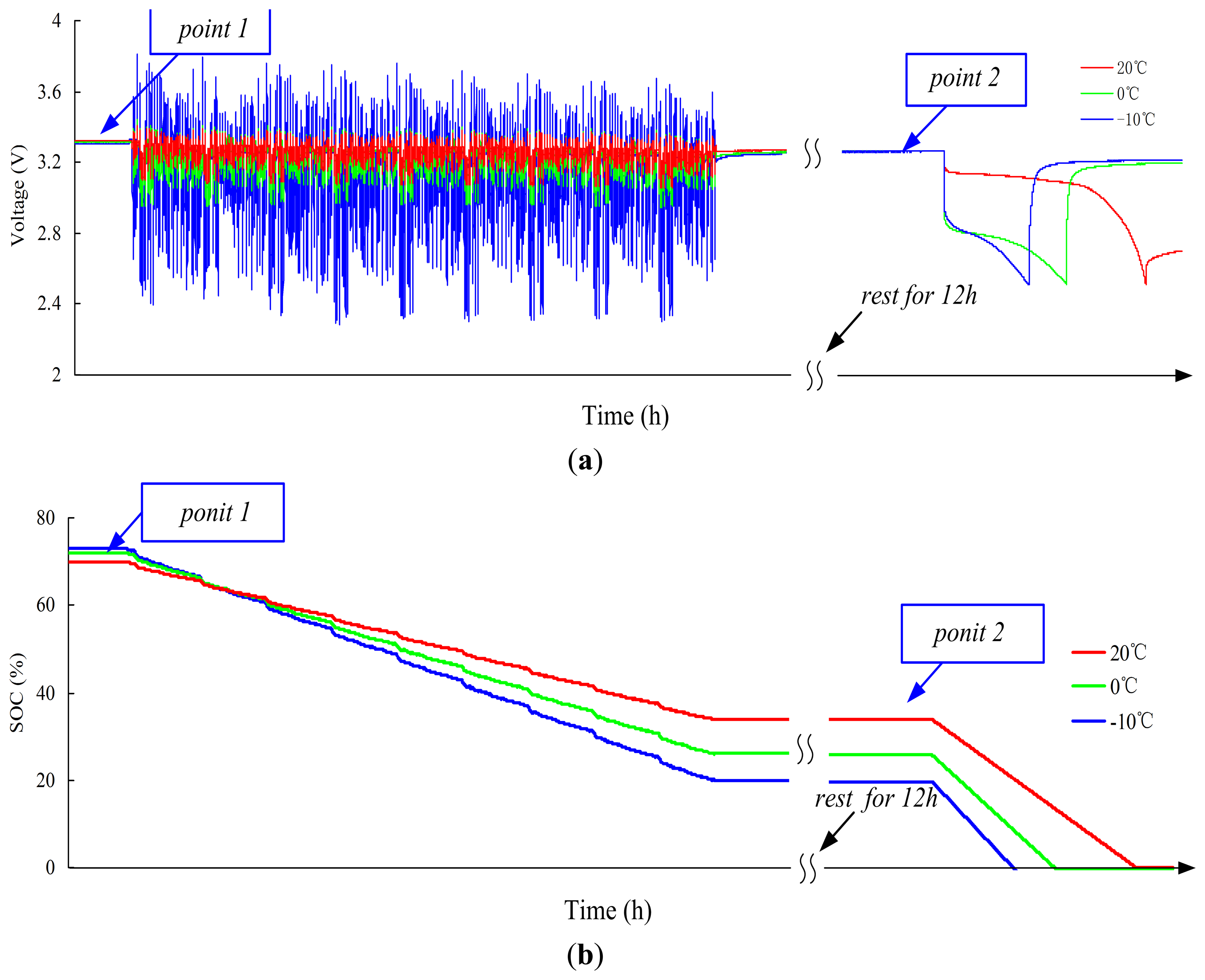
Figure 19a shows the voltage curves of constant temperature test at −10, 0, and 20 °C. Although the same Ah is charged before nine FUDS cycles (point 1), the releasable capacity at −10 °C or 0 °C is <20 °C in step (3). This phenomenon occurs because the available capacity decreases at low temperature. Figure 19b shows the SOC curves of constant temperature test at −10, 0, and 20 °C. The cell reaches point 1 through the R–L temperature path. The R–L non-rated initial SOCs at point 1 are estimated using the R–L non-rated OCV–SOCs.
Under the condition of known SOCIR,20 °C = 70%, SOCIR,0 °C and SOCIR,−10 °C can be calculated according to Equation (18), which are considered as the truth values of SOC at different temperatures. The errors of initial SOCs at different temperatures can be calculated according to the truth values of SOC. The results at point 1 are presented in Table 7. After nine FUDS cycles and before discharging (point 2), the cell undergoes the L–L temperature path. According to the L–L non-rated OCV–SOCs, we can estimate the L–L non-rated initial SOCs. Considering the truth values of SOC at point 1 as the initial SOCs, the non-rated SOCs can be calculated using Equation (12) during the nine FUDS cycles. Finally, the truth values of SOC at point 2 are measured using the discharge test method, by which the errors of L–L non-rated initial SOCs and non-rated SOCs can be calculated. The results at point 2 are reported in Table 8.
As shown in Tables 7 and 8, the errors of initial SOCs in different temperature paths are <3%. The calculation of non-rated SOCs during nine FUDS cycles produces subtle errors caused by the neglect of the influence of current on coulombic efficiency.
6.2. Alternated Temperature Test
The alternated temperature test is used to validate the performance of the Ah counting (SOCAh) and initial SOC (SOCOCV) estimation under alternated temperature condition. The procedures of alternated temperature test are as follows: (1) pre-test (the same as the −10 °C pre-test at constant temperature); (2) nine FUDS cycles are loaded to the cell, and the cell is discharged using the constant current of C/3 rate until bottom cut-off voltage is reached; (3) the cell is soaked at 20 °C for 12 h; and (4) additional two FUDS cycles are loaded to the cell, and then the cell is discharged using the constant current of C/3 rate until bottom cut-off voltage is reached.
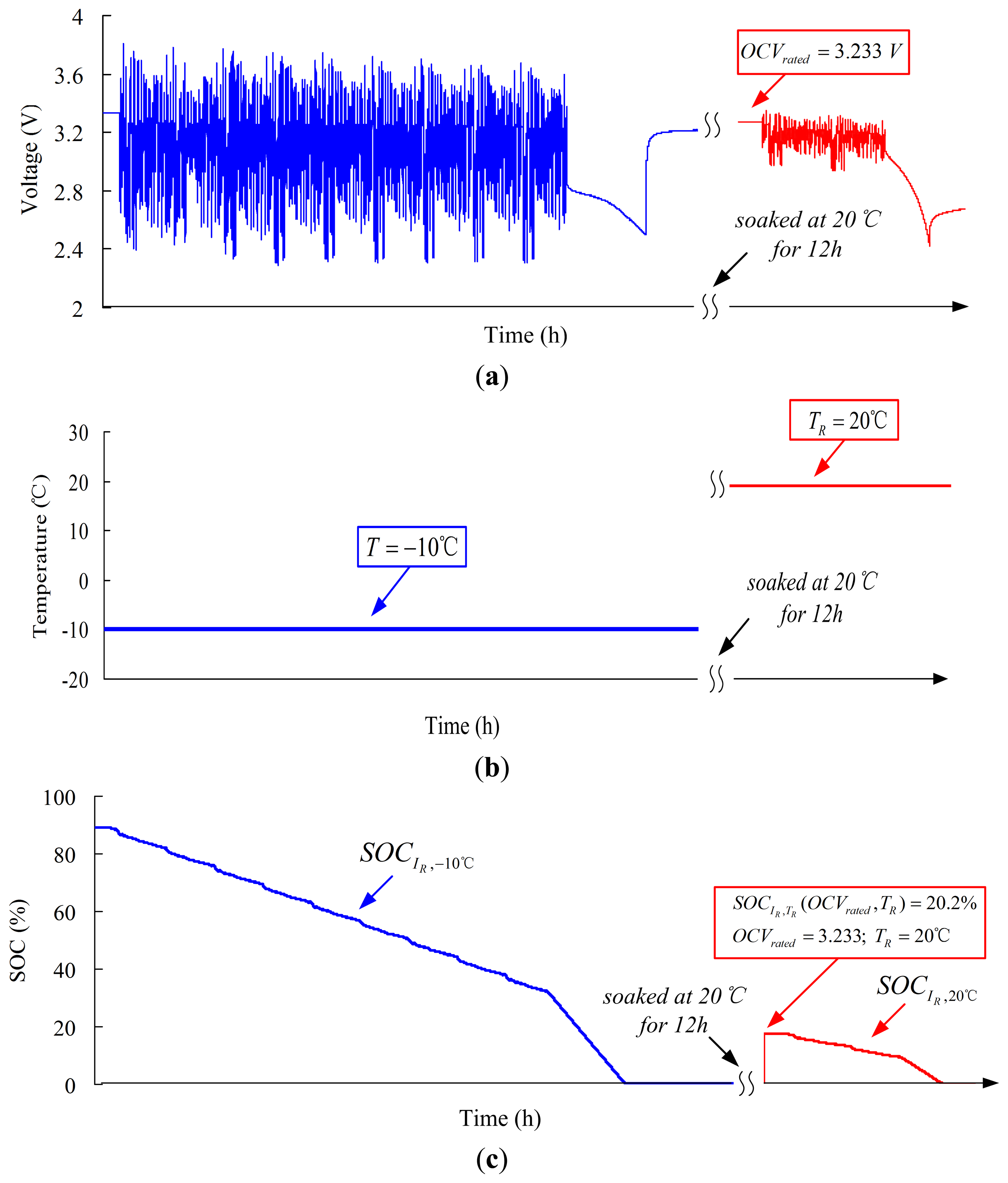
In the alternated temperature test, voltage, temperature, and SOC are depicted in Figure 20. Figure 20a shows the voltage curves of alternated temperature test. The cell has been discharged completely at −10 °C. However, the cell can be still discharged after 12 h at 20 °C due to the increase in available capacity. Figure 20b shows the temperature curves of alternated temperature test. The ambient temperature increases from −10 °C to 20 °C during the test. Figure 20c shows the SOC curves of alternated temperature test. After nine FUDS cycles, the cell is discharged and emptied at −10 C. The SOC at this moment is SOCIR,−10 °C = 0%. After being soaked at 20 °C for 12 h, SOCIR,−10 °C = 0% is converted into SOCIR,20 °C = 22% using Equation (18). Before the two FUDS cycles, the measured OCV at 20 °C is OCVrated = 3.233 V. According to the rated OCV–SOCs, we can estimate the rated initial SOC at SOCIR,TR(OCVrated,TR) = 20.2%. Finally, the true value of SOC is 21.7%, which is measured by Ah counting until the cell is discharged completely. The errors of rated initial SOC and rated SOC are both <2%.
7. Conclusions
Ambient temperature significantly influences the characteristics of lithium-ion batteries, such as capacity, coulombic efficiency, and OCV. Such temperature effects cause direct errors in SOC estimation. In this paper, we propose a combined SOC algorithm to address the temperature dependence of battery characteristics. First, our method simply and effectively improves the accuracy of the estimated SOC for lithium-ion batteries at different ambient temperatures. With minimal calculations this method can be used in BMS for on-board estimation. Second, the data of battery characteristics are obtained using the uncomplicated battery test from −20 to 20 °C, with a temperature interval of 10 °C. If the method is flexible in a wider temperature range or higher temperature resolution, the tests are only implemented under the corresponding temperature. Finally, two dynamic loading tests are conducted on the battery under constant and alternated temperatures to assess the SOC estimation performance using the proposed approach. The results indicate that the rated/non-rated initial SOC estimation based on the rated/non-rated OCV–SOCs in different temperature paths provides accurate values to calibrate the SOC estimated by Ah counting. In addition, the conversion of SOC between different temperatures exhibits high accuracy. The two SOC algorithms at different ambient temperatures have good consistency. Thus, this approach could be used in actual vehicle applications. Further studies on the following two aspects are recommended. First, advanced algorithms with the battery model under different temperatures can be applied to estimate on-line, real-time, and closed-loop SOC. Second, if this method is to be developed for SOC estimation of battery packs, other problems, such as the variation of cells, should be considered.
Acknowledgments
This research was supported by the National High Technology Research and Development Program of China (grant No. 2012AA111003) in part and the National Energy Technology Research and Application of Engineering Demonstrative Project of China (grant No. NY20110703-1) in part. The author would also like to thank the reviewers for their corrections and helpful suggestions.
Conflicts of Interest
The authors declare no conflict of interest.
References
- Scrosati, B.; Garche, J. Lithium batteries: Status, prospects and future. J. Power Sour. 2010, 195, 2419–2430. [Google Scholar]
- Lu, L.G.; Han, X.B.; Li, J.Q.; Hua, J.F.; Ouyang, M.G. A review on the key issues for lithium-ion battery management in electric vehicles. J. Power Sour. 2013, 226, 272–288. [Google Scholar]
- Wang, J.; Cao, B.; Chen, Q.; Wang, F. Combined state of charge estimator for electric vehicle battery pack. Control Eng. Pract. 2007, 15, 1569–1576. [Google Scholar]
- Dubarry, M.; Svoboda, V.; Hwu, R.; Liaw, B.Y. Capacity loss in rechargeable lithium cells during cycle life testing: The importance of determining state-of-charge. J. Power Sour. 2007, 174, 1121–1125. [Google Scholar]
- Pop, V.; Bergveld, H.J.; Op het Veld, J.H.G.; Regtien, P.P.L.; Danilov, D.; Notten, P.H.L. Modeling battery behavior for accurate state-of-charge indication. J. Electrochem. Soc. 2006, 153, A2013–A2022. [Google Scholar]
- Pop, V.; Bergveld, H.J.; Notten, P.H.L.; Regtien, P.P.L. State-of-the-art of battery state-of-charge determination. Meas. Sci. Technol. 2005, 16, R93–R110. [Google Scholar]
- Iryna, S.; William, R.; Evgeny, V.; Belfadhel-Ayeb, A.; Notten, P.H.L. Battery open-circuit voltage estimation by a method of statistical analysis. J. Power Sour. 2006, 159, 1484–1487. [Google Scholar]
- Gu, W.B.; Wang, C.Y. Thermal-electrochemical modeling of battery systems. J. Electrochem. Soc. 2000, 147, 2910–2922. [Google Scholar]
- Domenico, D.D.; Fiengo, G.; Stefanopoulou, A. Lithium-Ion Battery State of Charge Estimation with a Kalman Filter Based on an Electrochemical Model. Proceedings of the 17th IEEE International Conference on Control Applications, San Antonio, TX, USA, 3–5 September 2008; pp. 702–707.
- Speltino, C.; Di Domenico, D.; Fiengo, G.; Stefanopoulou, A. Comparison of reduced order lithium-ion battery models for automotive applications. Proceedings of the 48th IEEE Conference on Decision and Control, 2009 Held Jointly with the 2009 28th Chinese Control Conference (CDC/CCC), Shanghai, China, 15–18 December 2009; pp. 3276–3281.
- Chan, C.C.; Lo, E.W.C.; Weixiang, S. Available capacity computation model based on artificial neural network for lead-acid batteries in electric vehicles. J. Power Sour. 2000, 87, 201–204. [Google Scholar]
- Liao, E.H. Neural network based SOC estimation algorithm of LiFePO4battery in EV. Master Dissertation, University of Electronic Science and Technology Of China, ChengDu, China, 2011. [Google Scholar]
- Lee, Y.S.; Wang, J.; Kuo, T.Y. Lithium-ion battery model and fuzzy neural approach for estimating battery state of charge. Proceedings of the International Electric Vehicle Symposium, World Electric Vehicle Association, Busan, Korea, 6–9 October 2002; pp. 1879–1890.
- Chau, K.T.; Wu, K.C.; Chan, C.C. A new battery capacity indicator for lithium-ion battery powered electric vehicles using adaptive neuro-fuzzy inference system. Energy Convers. Manag. 2004, 45, 1681–1692. [Google Scholar]
- Singh, P.; Vinjamuri, R.; Wang, X.; Reisner, D. Design and implementation of a fuzzy logic-based state-of-charge meter for Li-ion batteries used in portable defibrillators. J. Power Sour. 2006, 162, 829–836. [Google Scholar]
- Wang, J. Estimation of dynamic battery soc using fuzzy arithmetic and the realization on DSP. Master Dissertation, Jilin University, Changchun, China, 2007. [Google Scholar]
- Cuadras, A.; Kanoun, O. SOC Li-ion battery monitoring with impedance spectroscopy. Proceedings of the Sixth IEEE International Multi-Conference on Systems, Signals and Devices, Djerba, Tunisia, 23–26 March 2009; Volume 5, pp. 1–5.
- Huet, F. A review of impedance measurements for determination of the state-of-charge or state-of-health of secondary batteries. J. Power Sour. 1998, 70, 59–69. [Google Scholar]
- Rodrigues, S.; Muichandraiah, N.; Shukla, A.K. Review of state-of-charge indication of batteries by means of a.c. impedance measurements. J. Power Sour. 2000, 87, 12–20. [Google Scholar]
- Johnson, V.H.; Pesaran, A.A.; Sack, T.; America, S. Temperature-dependent battery models for high-power lithium-ion batteries. Proceedings of the 17th Annual Electric Vehicle Symposium, Montreal, QC, Canada, 15–18 October 2000; pp. 1–14.
- Xing, Y.J.; He, W.; Pecht, M.; Tsui, K.L. State of charge estimation of lithium-ion batteries using the open-circuit voltage at various ambient temperatures. Appl. Energy 2014, 113, 106–115. [Google Scholar]
- Ng, K.S.; Moo, C.-S.; Chen, Y.-P.; Hsieh, Y.-C. Enhanced coulomb counting method for estimating state-of-charge and state-of-health of lithium-ion batteries. Appl. Energy 2009, 86, 1506–1511. [Google Scholar]
- Li, I.H.; Wang, W.Y.; Su, S.F.; Lee, Y.S. A merged fuzzy neural network and its applications in battery state-of-charge estimation. IEEE Trans. Energy Conv. 2007, 22, 697–708. [Google Scholar]
- Cheng, B.; Bai, Z.F.; Cao, B.G. State of charge estimation based on evolutionary neural network. Energy Convers. Manag. 2008, 49, 2788–2794. [Google Scholar]
- Wang, J.; Chen, Q.; Cao, B. Support vector machine based battery model for electric vehicles. Energy Convers. Manag. 2006, 47, 858–864. [Google Scholar]
- Plett, G.L. Extended Kalman filtering for battery management systems of LiPBbased HEV battery packs: Part 2. Modeling and identification. J. Power Sour. 2004, 134, 262–276. [Google Scholar]
- Plett, G.L. Sigma-point Kalman filtering for battery management systems of LiPB-based HEV Battery packs: Part 2. Simultaneous state and parameter estimation. J. Power Sour. 2006, 161, 1369–1384. [Google Scholar]
- Hu, X.; Li, S.; Peng, H. A comparative study of equivalent circuit models for Li-ion batteries. J. Power Sour. 2011, 198, 359–367. [Google Scholar]
- Chang, M.H.; Huang, H.P.; Chang, S.W. A New State of Charge Estimation Method for LiFePO4 Battery Packs Used in Robots. Energies 2013, 6, 2007–2030. [Google Scholar]
- Roscher, M.A.; Sauer, D.U. Dynamic electric behavior and open-circuit-voltage modeling of LiFePO4-based lithium ion secondary batteries. J. Power Sour. 2011, 196, 331–336. [Google Scholar]
- Pesaran, A.A.; Markel, T.; Tataria, H.S.; Howell, D. Battery Requirements for Plug-in Hybrid Electric Vehicles—Analysis and Rationale. Proceedings of the 23rd International Electric Vehicle Symposium (EVS-23), Anaheim, CA, USA, 2–5 December 2007; pp. 1–15.
- Zhang, S.S.; Xu, X.; Jow, T.R. The low temperature performance of Li-ion batteries. J. Power Sour. 2003, 115, 137–140. [Google Scholar]
- Hunt, G. USABC Electric Vehicle Battery Test Procedures Manual; United States Department of Energy: Washington, DC, USA, 1996. [Google Scholar]
- Idaho National Engineering; Environmental Laboratory. Battery Test Manual for Plug-in Hybrid Electric Vehicles; Assistant Secretary for Energy Efficiency and Renewable Energy (EERE) Idaho Operations Office: Idaho Falls, ID, USA, 2010. [Google Scholar]
- Weather China. Available online: http://www.weather.com.cn/weather/101050101.shtml (accessed on 13 February 2014).
- Sato, N. Thermal behavior analysis of lithium-ion batteries for electric and hybrid vehicles. J. Power Sour. 2001, 99, 70–77. [Google Scholar]
- Lee, S.J.; Kim, J.H.; Lee, J. State-of-charge and capacity estimation of lithium-ion battery using a new open-circuit voltage versus state-of-charge. J. Power Sour. 2008, 185, 1367–1373. [Google Scholar]
- Ye, Y.H.; Shi, Y.X.; Cai, N.S.; Lee, J.J.; He, X.M. Electro-thermal modeling and experimental validation for lithium ion battery. J. Power Sour. 2012, 199, 227–238. [Google Scholar]


| Temperature (°C) | First (Ah) | Second (Ah) | Third (Ah) | Average (Ah) |
|---|---|---|---|---|
| 20 | 100 | 100 | 99 | 100 |
| 10 | 98 | 98 | 98 | 98 |
| 0 | 83 | 82 | 82 | 82 |
| −10 | 67 | 66 | 65 | 66 |
| −20 | 32 | 32 | 32 | 32 |
| Temperature (°C) | LFD (Ah) | Capacity (Ah) | LFC (Ah) |
|---|---|---|---|
| 20 | 0 | 100 | 0 |
| 10 | 1 | 98 | 1 |
| 0 | 11 | 82 | 7 |
| −10 | 22 | 66 | 12 |
| −20 | 47 | 32 | 21 |
| Cha | Dis | |||
|---|---|---|---|---|
| Standard | Non-standard | |||
|---|---|---|---|---|
| 1 | ||||
| 1 | - | |||
| 1 | - | - | ||
| 1 | - | - | - | |
| Standard | Non-standard | |||
|---|---|---|---|---|
| 1 | ||||
| 1 | - | |||
| 1 | - | - | ||
| 1 | - | - | - | |
| Temperature (°C) | True SOC (%) | R-L OCV (V) | R-L Initial SOC (%) | R-L Initial SOC Error (%) |
|---|---|---|---|---|
| 20 | 70 | 3.319 | 71.9 | 1.9 |
| 0 | 71.9 | 3.316 | 69.4 | −2.5 |
| −10 | 72.7 | 3.306 | 70.4 | −2.3 |
| Temperature (°C) | True SOC (%) | L-L OCV (V) | L-L Initial SOC (%) | L-L Initial SOC Error (%) | Non-Rated SOC (%) | Non-Rated SOC Error (%) |
|---|---|---|---|---|---|---|
| 20 | 33.4 | 3.270 | 32.1 | −1.3 | 34.3 | 0.9 |
| 0 | 25.8 | 3.269 | 26.6 | 0.8 | 27.0 | 1.2 |
| −10 | 20.6 | 3.267 | 19.4 | −1.2 | 19.9 | −0.7 |
© 2014 by the authors; licensee MDPI, Basel, Switzerland. This article is an open access article distributed under the terms and conditions of the Creative Commons Attribution license ( http://creativecommons.org/licenses/by/3.0/).
Share and Cite
Feng, F.; Lu, R.; Zhu, C. A Combined State of Charge Estimation Method for Lithium-Ion Batteries Used in a Wide Ambient Temperature Range. Energies 2014, 7, 3004-3032. https://doi.org/10.3390/en7053004
Feng F, Lu R, Zhu C. A Combined State of Charge Estimation Method for Lithium-Ion Batteries Used in a Wide Ambient Temperature Range. Energies. 2014; 7(5):3004-3032. https://doi.org/10.3390/en7053004
Chicago/Turabian StyleFeng, Fei, Rengui Lu, and Chunbo Zhu. 2014. "A Combined State of Charge Estimation Method for Lithium-Ion Batteries Used in a Wide Ambient Temperature Range" Energies 7, no. 5: 3004-3032. https://doi.org/10.3390/en7053004