Analysis of the Energy Balance of Shale Gas Development

Abstract

Interest has rapidly grown in the use of unconventional resources to compensate for depletion of conventional hydrocarbon resources (“easy hydrocarbon”) that are produced at relatively low cost from oil and gas fields with large proven reserves. When one wants to ensure the prospects for development of unconventional resources that are potentially vast in terms of their energy potential, it is essential to determine the quality of that energy. Here we consider the development of shale gas, an unconventional energy resource of particularly strong interest of late, through analysis of its energy return on investment (EROI), a key indicator for qualitative assessment of energy resources. We used a Monte Carlo approach for the carbon footprint of U.S. operations in shale gas development to estimate expected ranges of EROI values by incorporating parameter variability. We obtained an EROI of between 13 and 23, with a mean of approximately 17 at the start of the pipeline. When we incorporated all the costs required to bring shale gas to the consumer, the mean value of EROI drops from about 17 at the start of the pipeline to 12 when delivered to the consumer. The shale gas EROI values estimated in the present study are in the initial stage of shale gas exploitation where the quality of that resource may be considerably higher than the mean and thus the careful and continuous investigation of change in EROI is needed, especially as production moves off the initial “sweet spots”.

1. Introduction

In 2008, the U.S. surpassed Russia in natural gas (NG) production to become the world's largest producer, with unconventional NG (tight-sand gas, coal-bed methane, and shale gas) production accounting for more than 50% of its total production output. Shale gas production in particular has followed a sharply upward trend recently. In 2011, shale gas accounted for approximately 30% of the total NG production in the U.S., clearly indicating the strong state of U.S. shale gas development. Energy resources that require higher or at least new levels of technology and higher cost for extraction than conventional resources are generally called “unconventional resources”. Advances in resource development technologies enable development of unconventional NG that are abundant in volume. The expanding development of unconventional resources, with their huge reserves, will have a strong, far-reaching impact. In the long-range view of energy supply and demand, it is generally held that the advent of unconventional resources will enable us to meet the needs in terms of quantity, even when confronted by depletion of “easy hydrocarbon resources” that can be produced at relatively low cost from oil and gas fields holding huge proven reserves.

Various studies have been made over the past half century on qualitative assessment of the degree to which the use of our energy resources can actually contribute to society. Systems ecologist H. T. Odum, known as the progenitor of qualitative energy assessment, first advanced the concept of “net energy” in the 1970s, which is essentially the energy obtained from an energy source minus the energy used in its acquisition and concentration (the energy investment, or energy cost). Odum proposed in 1973 that “the true value of energy source is the net energy” [1]. In this view, for an organism to leave its own seed to subsequent generations, it must evolve to adapt to changes in its environment and reproductive activities, which in itself requires additional energy. Taking this energy usage into account, if the organism cannot obtain net energy, then it cannot survive. In biological terms, the securement of net energy is thus essential, and a prerequisite for the evolution of organisms (Hall et al. [2]). Hall and Cleveland applied the net energy concept to oil development in the U.S. [3], and Cleveland et al. [4] and Hall et al. [5] performed analyses using EROI (energy return on investment) as a key indicator [6]. EROI is defined as the ratio of the total energy gained from an energy production process to the energy invested in its acquisition. EROI analysis a very powerful tool for evaluating various energy sources. However, one should note that EROI by itself is not necessarily sufficient for policy decisions; rather, it is just the tool we prefer the most, especially when EROI analyses show stark differences among competing energy sources (Murphy and Hall [6]).

In the midst of the heightening worldwide interest in unconventional resources, we focus here on the especially rapidly expanding shale gas development in the U.S., and apply a scientific approach to calculate the EROI of shale gas development. Aucott and Melillo [7] preliminarily estimated the EROI of shale gas obtained in the Marcellus Shale. They used estimates of carbon dioxide and nitrogen oxides emitted from the gas extraction processes as energy use, as well as fuel-use reports from industry and other sources. However, most of the fuel-use reports were obtained from personal communication. Available information about energy consumption in shale gas development is limited because energy companies generally do not provide detailed information on their energy consumption.

On the other hand, CO₂ emission data are more available due to regulations such as the mandatory greenhouse gas reporting rule. Weber and Clavin [8] compared six previous studies on the carbon footprints in shale gas development at different basins, excluded significant outlying values, derived statistical estimates for each emissions category, and on this basis provided what may be considered carbon footprint data on the average shale development operation in the U.S. Weber and Clavin [8] carefully discussed parameter variability and uncertainty of carbon footprint data to find some find some key factors affecting the estimates of carbon footprint data as follows: First, the six studies [9–14] analyzed different basins: National Energy Technology Laboratory (NETL) [11] examined only the Barnett shale basin, Jiang et al. [10] examined only the Marcellus shale basin, Stephenson et al. [12] and Burnham et al. [13] averaged over North American basins, and Hultman et al. [14] and Howarth et al. [9] averaged over all unconventional gas including tight gas. As described in Weber and Clavin [8], the basin choice affects both the estimated ultimate recovery of wells as well as the methane content of produced natural gas cited as 97% in Jiang et al. [10], 87% in Stephenson et al. [12], 80% in Burnham et al. [13], and 78% in NETL [11], Howarth et al. [9], and Hultman et al. [14]. Second, the six studies used different time periods of analysis, ranging from 3 years to 30 years, which causes immense uncertainty in estimated ultimate recovery (EUR). Weber and Clavin [8] created a Monte Carlo simulation using distributions for EUR (minimum = 0.5 bcf, most likely = 2 bcf, and maximum = 3.5 bcf). Clark et al. [15] mentioned that the EUR for a play is also subject to uncertainty and represents future well performance, which typically becomes more accurate as a play develops and more wells are drilled and produced. Third, the six studies adopted different methods of uncertainty quantification: none (Hultman et al. [14]), simple high-low ranges (Howarth et al. [9], Stephenson et al. [12], and NETL [11]), and Monte Carlo simulations with an 80% probability interval (Burnham et al. [13]) and 90% probability interval (Jiang et al. [10]). Fourth, Clark et al. [15] mentioned that the variability of water consumption is primarily driven by the quantity of hydraulic fracturing fluid used and the number of times a well is hydraulically fractured. The volume of fracturing fluid required can vary for a wide range of reasons including, but not limited to the length of the lateral portion of the well, the number of fracture stages, variations in the proprietary hydraulic fracturing practices used by service providers, and geological variability within and between plays [15].

Weber and Clavin [8] carefully examined six recent studies to produce a Monte Carlo uncertainty analysis of the carbon footprint of both shale and conventional natural gas production. Due to the scarcity of data, which is often common in life cycle assessment (LCA) studies on carbon footprint, one cannot obtain the true underlying distribution functions for a number of parameters. Instead Weber and Clavin [8] chose flexible triangular distributions with a most likely value equal to the average of the various study estimates. They chose a most likely value equal to either the average of the various study estimates or a single value judged to be of high quality and minimum/maximum values equal to the minimum and maximum study estimates for each emissions subcategory. The carbon footprints used in the present study as data for calculation of the shale gas EROI are taken from the estimates of Weber and Clavin [8]. To convert carbon footprint data to energy equivalents, we add the emission factor (defined by the carbon dioxide emission per calorific value) into the Monte Carlo simulation which can derive statistical information from uncertain data. We derive the ranges of expected EROI values from the Monte Carlo simulation. Furthermore, the results of EROI of shale gas are compared with those of conventional natural gas (NG) for onshore development in the U.S.

In our calculation of the EROI, we adopt different methods from Aucott and Melillo [7], which provides an opportunity under many uncertainties to validate the estimation of the shale gas EROI. We adjust both the protocol for calculation of EROI and the system boundary on EROI calculations in the present study so as to coincide with those of Aucott and Melillo. The present study also contributes to analysis of uncertainties in EROI estimation by comparing the two different approaches. Furthermore, the difference between Aucott and Melillo [7] and the present study is that the present study obtains the statistical value of EROI on the average shale development operation in the U.S. while Aucott and Melillo [7] conducted an analysis of EROI of shale gas only in the Marcellus Shale.

2. Methods

We derived energy use for the production of shale gas by converting readily available carbon release data into the energy use associated with that release. This was necessary because the energy used for the production of shale gas is not made available. Because there are legal requirements for providing information on the amount of carbon released by shale gas facilities we converted these values to energy inputs and gas produced to generate an estimate of EROI. We include a statistical analysis of the uncertainty in these estimates. Details follow.

2.1. Carbon Footprint in Shale Gas and Conventional NG Development

Expectations are high for the future of shale gas development, but it is also viewed as problematic in its potential for water and atmospheric pollution and its effect on climate change through the release of methane and other gases during its production, particularly in regard to the greenhouse effect of methane escaping to the atmosphere. The carbon footprint of a given activity is the total volume of carbon dioxide and other greenhouse gases directly and indirectly released in the course of that activity over its entire life cycle (i.e., from initiation of exploration to closing of the field), as calculated once the sources of this release have been identified. The outline of the methodology of Weber and Clavin [8] for estimation of the carbon footprint in shale gas development was as follows.

As described above, the six different studies cited by Weber and Clavin [8] all shared the objective of calculating the carbon footprint of shale gas development, but differed in scope (range of investigation) as relating to assumed development regions, methane content of the gas, and other aspects. Acknowledging these regional differences, Weber and Clavin [8] applied the data from all six studies to infer an average for the shale gas development implementations in the U.S. Weber and Clavin [8] examined the assumptions and boundary conditions of six published studies [9–14] on the carbon footprint of shale gas development, unified these carbon footprint data, and submitted their unified data and assumptions to Monte Carlo simulation using a selected combination of the inputs taken from across the six studies, summed together to create category subtotal (preproduction, production, and transmission). To unify these six studies with different scopes, basins, time periods of analysis, system boundaries, and uncertainty quantification, Weber and Clavin [8] allowed the widest possible inclusion of foreseeable causes of greenhouse gases and in some cases adjustments were added to the study results so that the system boundaries accorded with a broad system boundary to include all potential sources identified in any of the studies. Furthermore, they excluded as outliers the data that included values that diverged excessively from the other values by citing the data of calculations by Venkatesh et al. [16]. They also compared the carbon footprints obtained for shale gas development with those of conventional natural gas (NG) development [8]. Following established practice, they used gCO₂e/MJLHV (grams of carbon dioxide equivalent per Mega Joule Lower Heating Value), based on calorific value, as the functional unit for upstream and downstream operations and gCO₂e/kWh, based on electric energy, as the functional unit for future emissions from the power plant. The LHV is defined as the amount of heat produced when combusting a certain amount of fuel assuming all water is in the form of steam and is not condensed (Finet [17]). Through these processes, Weber and Clavin [8] determined the most likely, minimum, and maximum values as input values to Monte Carlo simulation for each emission category as shown in

Table 1. Input parameters to Monte Carlo simulation for each category of emission in shale gas and conventional NG development using six published studies (Weber and Clavin [8]). Units: gCO₂e/MJ (grams of carbon dioxide equivalent per mega joule) unless otherwise indicated.

			Minimum	Most likely	Maximum
Preproduction	Well pad construction a		0.05	0.13	0.3
	Well drilling b		0.1	0.2	0.4
	Fracking water c		0.04	0.23	0.5
	Fracking chemicals d		0.04	0.07	0.1
	Well completion (conventional) e		0.01	0.12	0.41
	Fugitive emission during well completion (shale gas) f	Total emission [Mton CH4]	13.5	177	385
		Flare combustion ratio	0.15	0.41	1
		Estimated ultimate recovery (EUR) [billion ft3]	0.5	2	5.3
Production/Processing	Flaring g		0	0.43	1.3
	Lease/plant energy (conventional) h		2	3.3	4.3
	Lease/plant energy (shale gas) i		2	3.3	4.1
	Vented CO2 at plant j		0.2	0.7	2.8
	Fugitive at well k		0.7	2.3	5.0
	Fugitive at plant l		0.7	1.0	3.6
	Liquid unloading (conventional NG well) m		0.6	4.1	6.6
Transmission	Compression fuel n		1	1.7	2.7
	Fugitive transmission o		0.2	0.38	0.6
	Mean		0.55	1.28	2.34

^aHere, it is assumed that the carbon footprint from the preparation of well pad comprises carbon loss due to vegetation loss and emissions (as calculated from monetary cost) resulting from roadway and pad construction [10];^bThe carbon footprint of the well drilling operation is calculated, under the assumption that it comprises emissions resulting from energy consumption in drilling, the acquisition and processing of drilling mud (the main component in the drilling mud is bentonite), and water usage [10];^cThe carbon footprint of allocating the water necessary when fracking is calculated, as a process specific to shale gas development;^dThe carbon footprint for acquisition of the chemicals necessary in fracking is calculated as a process specific to shale gas development. Jiang et al. [10] calculated the cost of procurement based on the quantities and prices of the materials used in fracking and converted it to carbon dioxide emission to obtain the carbon footprint;^e,fJiang et al. [10] and Stephenson et al. [12] calculated the carbon footprint of this process from the methane release and the carbon dioxide generation due to incomplete combustion in flaring during the initial stage of production;^gFlaring refers to the burning of gases accompanying oil or gas production in a tower installed in the facility. Its effects include preventing explosions and untreated methane gas released to the atmosphere. Methane gas has a strong greenhouse effect; its global warming potential is 21 times that of carbon dioxide. In this study, the carbon footprint of flaring is calculated in terms of its carbon dioxide generation;^h,iThis involves the energy consumed at both the production site (lease fuel) and in the NG processing plant (plant fuel), which are generally regarded as difficult to consider separately. The methods of its calculation differ from study to study. In some the carbon footprint of toxic gas removal, compression, condensate separation, processing, and other processes are cumulatively calculated (NETL; U.S. National Energy Technology Laboratory [11], Stephenson et al. [12]) and in others past industrial studies are cited (Burnham et al. [13]);^jThe amount of carbon dioxide that is vented at the NG processing plant is calculated as the carbon footprint;^kFugitive gas calculation accounts for the carbon footprint of NG emissions from the well and well plant. Weber and Clavin note that although emissions from pipelines and malfunctions in pneumatic systems, dehydrators, compressors, AGR units, and other equipment may be regarded as its sources, the largest cause is valve leakage [8]. The methods of calculation may involve a process-base approach (NETL) or the use of greenhouse gas emissions data from the U.S. EPA (Environmental Protection Agency), API (American Petroleum Institute), GAO (Government Accountability Office), and other organizations (Hultman et al. [14], Burnham et al. [13], Stephenson et al. [12], Howarth et al. [9]). In this study, we calculate the “fugitive at well” as the NG release at the well during production;^lHere the gas release at the natural gas processing plant is calculated, in the same manner as described above;^mIn a mature conventional NG well, the intermittently produced water and buildup of condensates tend to block the NG flow, and it is therefore necessary to remove them. The methane expected to be released and burned at that time is calculated as a carbon footprint;ⁿThe energy used in compression of the NG for transport is considered. The amount of energy consumed in compressing the NG for pipeline transmission is estimated;^oGas release which occurs during transport from the plant to the end consumer (the power plant) is calculated. NG distribution for applications other than electricity generation are excluded from consideration.

.

In Table 1, the carbon intensity is expressed in terms of grams of carbon dioxide equivalent per mega joule of energy provided (gCO₂e/MJ). They chose a most likely value equal to either the average of the various study estimates or a single value judged to be of high quality and minimum/maximum values equal to the minimum and maximum study estimates for each emissions subcategory. They then used these values in a Monte Carlo simulation by producing 10,000 samples that followed the triangular distribution formed from the minimum, most likely, and maximum values shown for each category, and summed them to calculate the carbon footprints of shale gas and conventional NG. They chose a 95% interval to capture best- and worst-case scenarios exhibited in the tails of the various input parameters' distributions. Finally, they obtained simulation estimates of the probability distributions of carbon footprints. The statistical estimated values obtained by Weber and Clavin show a 95% probability interval using Monte Carlo analysis with probability distributions constructed using the estimates in all six studies. In this context, a Monte Carlo approach allows us to estimate ranges of expected values of LCA metrics by incorporating parameter variability with specified distribution functions.

2.2. Approach Used for Deriving EROI from Carbon Footprint

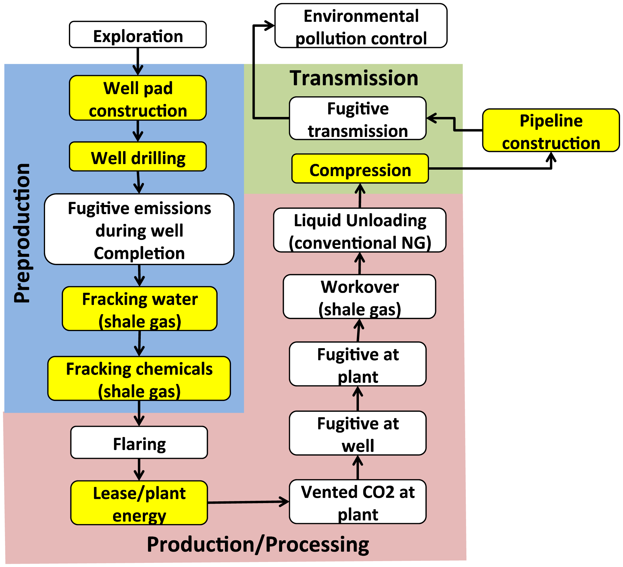
Figure 1 shows a flowchart of possible sources of greenhouse gas emissions in the course of development and production of shale gas and conventional NG, together with the emission categories defined by Weber and Clavin (Preproduction indicated by light blue, Production/Processing indicated by light pink, and Transmission indicated by light green). Furthermore, as shown by the system boundary of gas production processes in Figure 1, energy inputs taken into account by the present study are indicated by yellow boxes. Note that Weber and Clavin did not consider the category related to the pipeline construction and thus data for the pipeline construction are taken from the estimates of Aucott and Melillo [7]. Since the comprehensive methodology for calculating EROI is not entirely standardized, inclusions and boundaries of energy inputs should be clearly noted. Although EROI is usually calculated at the wellhead, our EROI estimation includes not only the energy consumption in gas production but also that energy used for toxic gas removal, compression, condensate separation, processing, and other factors related to transmission so as to coincide with the protocol for calculation of EROI and the system boundary on EROI calculations of Aucott and Melillo as possible.

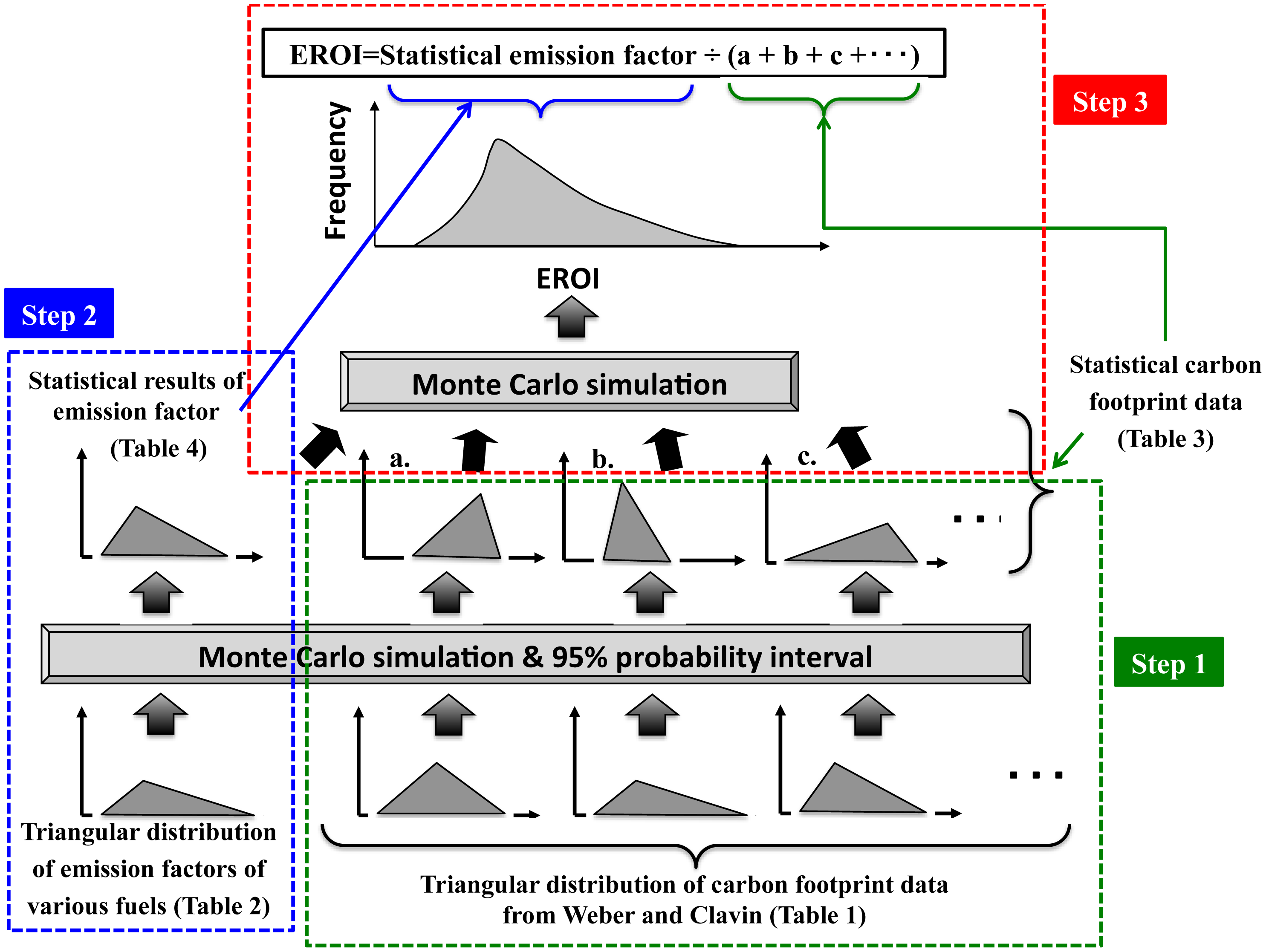
Figure 2 shows a schematic diagram of Monte Carlo simulation for the estimation of EROI conducted in the present study. Taking into account the uncertainties resulting from various factors like the regional differences in shale gas development, we opted to use a similar Monte Carlo simulation conducted in which random numbers are generated based on triangular distributions, after which an statistical solution was determined from the distribution of results. The procedure for this method is as follows:

Step 1

Similar to the method applied by Weber and Clavin as described above, to compute the quantified probability distribution of carbon footprint data of shale gas and conventional NG, we conducted a Monte Carlo simulation by producing 10,000 samples that followed the triangular distribution formed from the minimum, most likely, and maximum values shown for each category shown in Table 1. We also chose a 95% interval to obtain simulation estimates of the probability distributions of carbon footprints. We then determined triangular distributions with a most likely value equal to the mean value of the probability distributions and minimum/maximum values equal to the minimum and maximum of a 95% interval of the probability distributions for each emissions subcategory.

Step 2

We derived the statistical results of the emission factor defined as carbon dioxide emission per calorific value for fuel used in the course of gas development and production. Similarly, we conducted a Monte Carlo simulation by producing 10,000 samples that followed the triangular distribution formed from the minimum, most likely, and maximum values shown in

Table 2. Emission factors of various fuels used in generator (based on U.S. Energy Information Administration data [20]).

Fuel type	Values
Diesel fuel	73.15 kg CO2/MMBtu = 69.40 g CO2/MJ
Natural gas	53.06 kg CO2/MMBtu = 50.34 g CO2/MJ
Gasoline	71.26 kg CO2/MMBtu = 67.61 g CO2/MJ
Residual fuel	78.80 kg CO2/MMBtu = 74.76 g CO2/MJ

. As shown in Table 2, based on these values, we formed a triangular distribution with the NG, residual fuel, and diesel fuel emission factors as the minimum, maximum, and most likely, respectively. Electricity generation by engine is a common power source for drilling operations. The engines may be powered by NG, gasoline, residual fuel, or other fuel, as well as by diesel fuel (Website, U.S. industrial drilling equipment maker Flowtech Energy [18]). The use of NG at drilling sites is increasing in the U.S. because it is cheaper than diesel, for which its supply is sharply rising [19]. Similar to the Step 1, we chose a 95% interval to obtain simulation estimates of the probability distributions of the emission factor. We then determined triangular distributions with a most likely value equal to the mean value of the probability distributions and minimum/maximum values equal to the minimum and maximum of a 95% interval of the probability distributions.

Step 3

To compute the statistical distribution of EROI, we conducted a Monte Carlo simulation by producing 10,000 samples that followed the triangular distribution formed from the minimum, most likely, and maximum values of carbon footprints determined in the Step 1 and of the emission factor determined in the Step 2. We determine triangular distributions with a most likely value equal to the mean value of the probability distributions and minimum/maximum values equal to the minimum and maximum of a 95% interval of the probability distributions for each category.

In the present study, we derive two types of statistical results of EROI: EROI_{production/processing} EROI_transmission. The estimated value of EROI_{production/processing} includes the energy required in the category of preproduction and production/processing shown in Figure 2 while the value of EROI_transmission includes the energy required in the category of not only preproduction and production/processing but also transmission. To derive EROI_{production/processing} from carbon footprint data, we use the following equation:

$$\mathit{\text{ERO}}{I}_{\mathit{\text{production}}/\mathit{\text{processing}}}=\frac{e}{C{F}_{\mathit{\text{production}}/\mathit{\text{processing}}}}$$

(1)

where CF_{production/processing} is the statistical results of the total carbon footprint data [unit: g CO₂e/MJ] resulting from energy consumption calculated in Step 1 which are categorized in preproduction and production/processing shown in Figure 2 and e is the statistical results of the emission factor [unit: g CO₂e/MJ] for fuel used in the course of gas development and production calculated in Step 2. Thus, to obtain the probability distribution of a sort of EROIs, we opted to use a Monte Carlo simulation in which random numbers were generated according to the specific distribution of the carbon footprint resulting from energy consumption and the emission factors of the fuel used in the development and these values were substituted into Equation (1). Here we assume that random distributions of the carbon footprint resulting from energy consumption and the emission factors of the fuel used in the development satisfy the triangular distribution. In the present study, we performed 10,000 computing iterations in Monte Carlo simulation and output the results in terms of the mean, and maximum and minimum values showing a 95% probability interval, to represent the distribution.

Furthermore, to derive the statistical results of EROI_transmission which further include the energy cost for the pipeline construction, we use the following equation:

$$\mathit{\text{ERO}}{I}_{\mathit{\text{transmission}}}=\mathit{\text{Net\_gas\_factor}}/(1/\mathit{\text{ERO}}{I}_{\mathit{\text{production}}/\mathit{\text{processing}}}+{\mathit{\text{Input\_E}}}_{\mathit{\text{pipeline}}}/{\mathit{\text{Output\_E}}}_{\mathit{\text{ultimate}}})$$

(2)

where Net_gas_factor to be described later in detail is the ratio of the quantity of the net estimated ultimate recovery gas (given by the subtraction of the total quantity of flaring/vented/fugitive gases from the estimated ultimate recovery gas) to the quantity of the estimated ultimate recovery gas. Input_E_pipeline is the input energy value of the pipeline construction (i.e., 9637 GJ) obtained by Aucott and Melillo [7] and Output_E_ultimate is the estimated ultimate recovery (i.e., 3.25 × 10⁶ GJ) derived by Aucott and Melillo [7]. Although these values obtained by Aucott and Melillo were used in the development of shale gas, we used these values in the development of conventional gas.

3. Results

3.1. Simulation Estimates of the Probability Distributions of Carbon Footprints

Table 3. Comparison of statistical results of mean carbon footprints for each emissions category between conventional NG and shale gas. These results were derived from a Monte Carlo simulation using the triangular distribution formed from the minimum, most likely, and maximum values shown for each category shown in Table 1. The 95% probability interval is shown in parentheses for each category. Note that conventional NG is assumed to have the same carbon footprints related to energy inputs with the exception of those associated with hydraulic fracturing.

		Conventional gas	Shale gas
Preproduction	Well pad construction	0.16 (0.07–0.26)	0.16 (0.07–0.26)
	Well drilling	0.23 (0.12–0.36)	0.20 (0.12–0.36)
	Fracking water	-	0.26 (0.09–0.45)
	Fracking chemicals	-	0.07 (0.05–0.09)
	Fugitive emission during well completion	0.18 (0.04–0.37)	1.2 (0.2–3.4)
	Subtotal	0.57 (0.35–0.81)	1.9 (0.9–4.1)
Production/Processing	Flaring	0.6 (0.1–1.1)
	Lease/plant energy	3.2 (2.2–4.0)
	Vented CO2 at plant	1.2 (0.4–2.4)
	Fugitive at well	2.7 (1.1–4.5)
	Fugitive at plant	1.8 (0.8–3.2)
	Workover (shale gas well)	-	1.2 (0.0–4.8)
	Liquid unloading (conventional NG well)	3.8 (1.3–6.0)	-
	Subtotal	13.2 (9.6–16.7)	10.5 (7.2–15.3)
Transmission	Compression fuel	0.4 (0.2–0.6)
	Fugitive transmission	1.9 (1.2–2.5)
	Subtotal	2.2 (1.6–2.9)
Total		16.0 (12.4–19.5)	14.6 (11.0–21.0)

shows the comparison of statistical results of mean carbon footprints for each emissions category from Monte Carlo simulation between conventional NG and shale gas. In Table 3, as an indicator of uncertainty, the 95% probability interval is shown in parentheses for each category and their totals. These results are almost equivalent to those obtained by Weber and Clavin [8].

3.2. Simulation Estimates of Emission Factors of the Fuel Used in the Development

Table 4. Comparison of statistical results of emission factors derived from Monte Carlo simulation between conventional NG and shale gas. The 95% probability interval is shown in parentheses. Note that it is assumed that the mix of natural gas from conventional NG and shale gas creates the same GHG emission factor profile.

	Conventional NG		Shale gas
	Mean	95% probability interval	Mean	95% probability interval
Emission factor [g CO2e/MJ]	64.86	(54.00–72.97)	64.86	(54.00–72.97)

shows the statistical results of emission factors in shale gas and conventional NG development derived from Monte Carlo simulation. Note that it is assumed that the mix of natural gas from conventional NG and shale gas creates the same GHG emission factor profile. We also considered procurement of electricity from a power grid. According to the American Association of Drilling Engineers (AADE), this power mode has been investigated and practical development has been accomplished in an effort to reduce the greenhouse gas emission and noise and to hold down costs, as it has been found environmentally and economically sound [21]. In the U.S., the mean emission factor for electricity in 2009 was 551.4 g CO₂/kWh [22]. With a generating-end calorific value base of 8.78 MJ/kWh, primary energy conversion then yields an emission factor of 62.8 g CO₂/MJ. This is within the range generated with random numbers as described above for the diesel-engine emission factor, which indicates that electricity procurement from a power grid is covered by the range assumed for diesel-engine power procurement, and we therefore used the random numbers following the triangular distribution for the emission factor of engines as the emission factor for all of the conventional NG and shale gas development.

3.3. Statistical Results of EROI

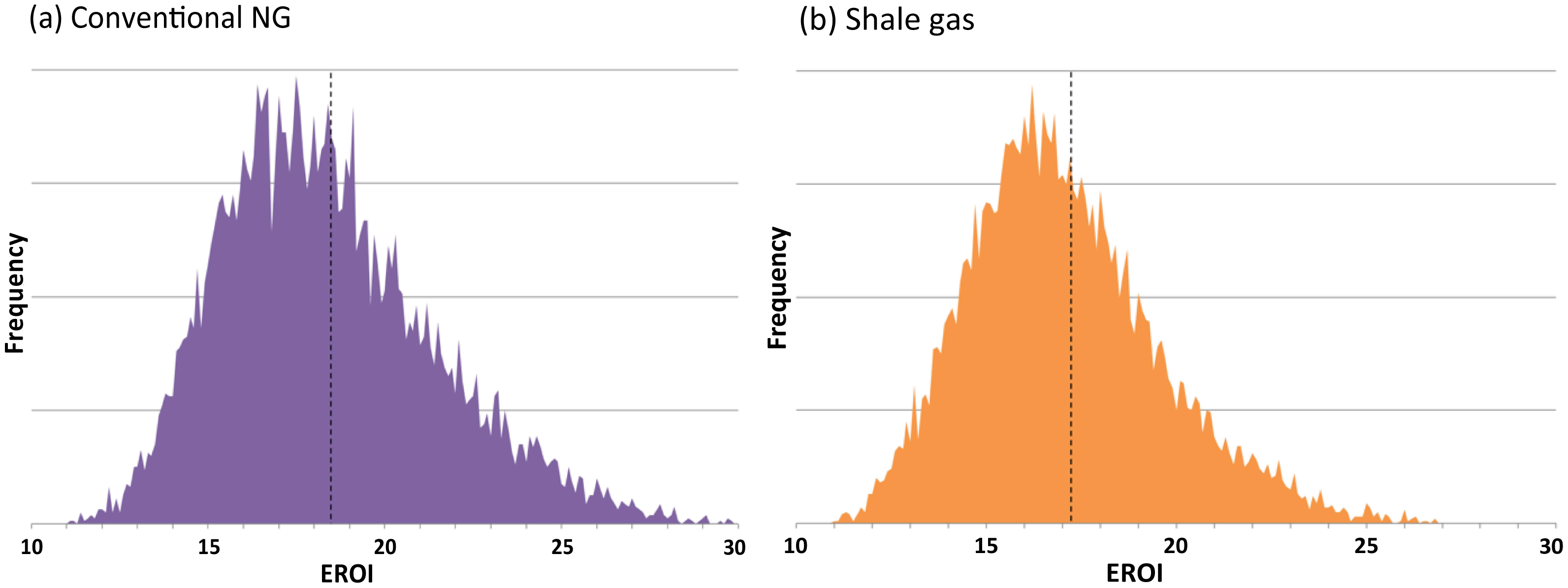
As shown by the statistical results of EROI_{production/processing} and EROI_transmission from Monte Carlo simulation in

Table 5. Comparison of statistical results of EROIs derived from Monte Carlo simulation between conventional NG and shale gas. The 95% probability interval is shown in parentheses.

	Conventional NG		Shale gas
	Mean	95% probability interval	Mean	95% probability interval
EROIproduction/processing	18	(14–25)	17	(13–23)
EROItransmission	13	(10–18)	12	(9–16)

, when we incorporated all the costs required to bring shale gas to the consumer, the mean value of EROI drops from about 17 at the start of the pipeline (i.e., EROI_{production/processing}) to 12 when delivered to the consumer (i.e., EROI_transmission). Similarly, in the case of conventional NG, the mean value of EROI drops from about 18 at the start of the pipeline to 13. In Table 5, as an indicator of uncertainty, the 95% probability interval is shown in parentheses. The EROI_{production/processing} distributions for conventional NG and shale gas are also shown graphically in Figure 3a,b, respectively.

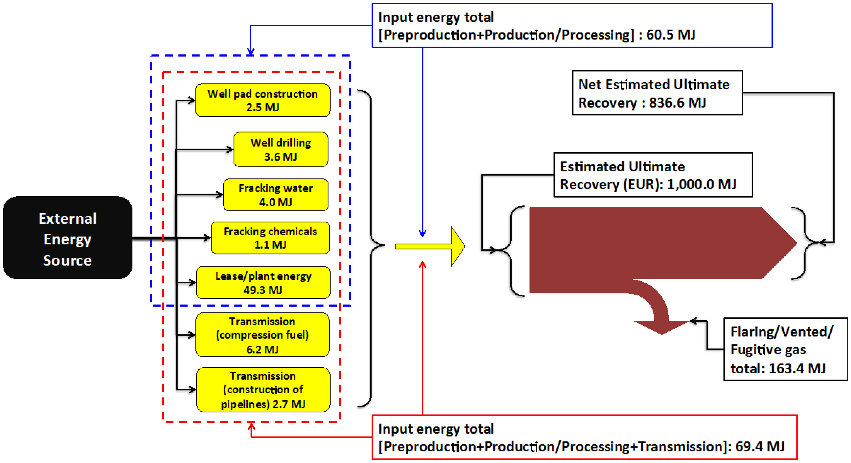
Nos. (1) through (14) of

Table 6. Energy investment [MJ] per GJ unit shale gas production for each category. Energy inputs taken into account by the present study are indicated by yellow filled.

		Item	Energy [MJ]	No.
Energy investment [MJ] per GJ shale gas production	Preproduction	Well pad construction	2.5	(1)
		Well drilling	3.6	(2)
		Fracking water	4.0	(3)
		Fracking chemicals	1.1	(4)
		Fugitive emissions during well completion	18.5	(5)
	Production/Processing	Flaring	9.3	(6)
		Lease/plant energy	49.3	(7)
		Vented CO2 at plant	18.5	(8)
		Fugitive at well	41.6	(9)
		Fugitive at plant	27.8	(10)
		Workover (shale gas well)	18.5	(11)
	Transmission	Transmission (compression fuel)	6.2	(12)
		Fugitive transmission	29.3	(13)
		Transmission (construction of pipelines) from Aucott and Melillo [8]	2.7	(14)
		Normalized Estimated Ultimate Recovery	1,000.0	(15)
		Input energy total [Preproduction + Production/Processing + Transmission] = (1) + (2) + (3) + (4) + (7) + (12) + (14)	69.4	(16)
		Input energy total [Preproduction + Production/Processing] = (1) + (2) + (3) + (4) + (7)	60.5	(17)
		Flaring/Vented/Fugitive gas total = (5) + (6) + (8) + (9) + (10) + (11) + (13)	163.4	(18)
		Net Estimated Ultimate Recovery =(15) − (18)	836.6	(19)
		Net_gas_factor = (15) ÷ (19) = 0.8366		(20)
		EROIproduction/processing = (15) ÷ (17) = 17		(21)
		EROItransmission = (19) ÷ (16) = 12		(22)

show the energy investment [MJ] per GJ unit shale gas production. In Nos. (1) through (13) of Table 6, the energy investment per GJ unit shale gas production in the present study was calculated by division of the mean value of carbon footprint data for each energy consumption category shown in Table 3 by the mean value of the emission factor (64.86 g CO₂e/MJ) shown in Table 4. In No. (14), the energy investment per GJ unit shale gas production in the category of construction of pipelines was calculated by division of the energy consumption required in the construction of pipelines (9637 GJ) by the typical estimated ultimate recovery (3.25 × 10⁶ GJ) derived by Aucott and Melillo [7]. In Table 6, Energy inputs taken into account by the present study are indicated by yellow filled. As we here assume GJ unit shale gas production, the calorific value of the normalized estimated ultimate recovery is 1000.0 MJ as shown in No. (15). We summed energy inputs required in the category of preproduction, production/processing, and transmission to calculate a total input energy in this category as shown in No. (16). Similarly, we summed energy inputs required in the category of preproduction and production/processing to calculate a total input energy in this category as shown in No. (17). Furthermore, we summed the energy losses due to flaring/vented/fugitive gases to calculate a total energy loss as shown in No. (18). Finally, we obtained the calorific value of the net estimated ultimate recovery as shown in No. (19) by subtracting the total energy losses caused by flaring/vented/fugitive gases shown in No. (18) from the calorific value of the estimated ultimate recovery shown in No. (15). As shown in No. (20), Net_gas_factor appeared in Equation (2) was calculated as 0.8366 by dividing the calorific value of the net estimated ultimate recovery shown in No. (19) by the calorific value of the estimated ultimate recovery shown in No. (15). The values of EROI_{production/processing} and EROI_transmission were calculated as 17 and 12 as shown in No. (21) and (22), respectively.

Figure 4 shows an energy flow diagram for shale gas development processes. In Figure 4, yellow boxes show energy inputs supplied by external energy sources such as NG, gasoline, residual fuel, and diesel fuel. In the present study, we do not consider the self-use of a produced fuel. Furthermore, we can see the decrease of the net quantity of produced gas due to fugitive and vent emissions from the estimated ultimate recovery (EUR). In Figure 4, the energy inputs for two types of EROI estimation can be graphically recognized by blue lines (EROI_{production/processing}) and red lines (EROI_transmission).

4. Discussion

4.1. Comparison of EROI of Various Oil and Gas Resources

As shown in

Table 7. Comparison of various oil and gas resource EROIs.

Type of energy		EROI	Source	Notes
Shale gas		17 (13–23)	Present study	EROI at the start of the pipeline
Shale gas		12 (9–16)	Present study	EROI at the consumer
Conventional NG		18 (14–25)	Present study	EROI at the start of the pipeline
Conventional NG		13 (10–18)	Present study	EROI at the consumer
Shale gas		64–112	Aucott and Melillo [7]	EROI based on NEER
Shale gas		8–12	Aucott and Melillo [7]	EROI based on NER
Oil & NG production	World (1992)	26	Gagnon et al. [24]	EROI at the wellhead
	World (2006)	18
	U.S. (1972)	19.9	Guilford et al. [25]	EROI at the start of the pipeline
	U.S. (2007)	10.7
	U.S., Gulf of Mexico	7–22	Moerschbaecher and Day Jr. [26]	EROI at the wellhead
NG	Canada, conventional	20	Freise [27]	EROI within a boundary including the exploration, drilling, gathering and separating stages
Other non- conventional resources	U.S. tight sand gas	67	Sell et al. [28]	EROI at the wellhead
	U.S. oil shale	1.1–1.8	Brandt [29]	EROI at the wellhead
	Methane hydrate	4–5	Callarotti [30]	Microwave heating of methane hydrate plugs in laboratory settings.

, the shale gas EROI obtained in this study generally equals or exceeds the EROIs reported for other types of oil and gas production, though it must be noted that the studies cited for the other oil and gas resources vary in systems boundaries of calculation. This comparison nevertheless indicates that shale gas production obtained from presently-exploited resources is not inferior to most other fuels from the perspective of EROI. However, we should note that the shale gas EROI values estimated in the present study are in the initial stage of shale gas exploitation and thus the careful and continuous investigation of change in EROI is needed, especially as production moves off the initial “sweet spots”.

Aucott and Melillo [7] performed an preliminary analysis of the EROI of shale gas development in the Marcellus Shale using two different protocols of EROI calculation: a net external energy ratio (NEER) and a net energy ratio (NER) termed by Brandt and Dale [23]. The NEER's denominator includes only energy inputs that are consumed from the existing industrial energy system, excluding any self-use energy and subtracts self-use energy from the total of the produced gas in the numerator while the NER includes any self-use energy in the denominator and subtracts self-use energy from the total of the produced gas in the numerator. Thus, the estimation results of EROI obtained by Aucott and Melillo are also shown in Table 7. The shale gas EROI of 64 to 112 obtained by the NEER (Aucott and Melillo) is far larger than the value of 8 to 12 by the NER (Aucott and Melillo). On the other hand, the present study includes the existing external energy in the denominator and as described above, we do not consider the self-use of a produced fuel. Anyhow, the protocol and the system boundary for calculation of EROI_transmission in the present study is almost equivalent to that of the NER values derived in Aucott and Melillo. The present study obtained the mean EROI_transmission value of approximately 12. This mean value is almost within the range of the NER value of 8 to 12 obtained by Aucott and Melillo.

Let us begin by examining calculation methods for energy investment, as used by Aucott and Melillo. In the summation approach by Aucott and Melillo, the energy investments include energy data on fuel used by each activity and other inclusions were calculated by multiplying related carbon footprint data and nitrogen oxides from gas extraction activities by the emission factor, and the energy indirectly invested in steel and other materials was then added to calculate the total energy investment.

Table 8. Comparison of energy investment [MJ] per GJ unit shale gas production.

		Present study	Aucott and Melillo [7]
Energy investment [MJ] per GJ shale gas production	Well pad construction	2.5	4.3
	Well drilling	3.6
	Fracking water	4.0	1.4
	Fracking chemicals	1.1
	Lease/plant energy	49.3	88.7
	Transmission (compression fuel)	6.2
	Transmission (construction of pipelines) from Aucott and Melillo [7]	2.7

shows a comparison of these results per GJ unit shale gas production with those of the present study. In Table 8, the energy investment per GJ unit shale gas production in the present study was calculated by division of the mean value of carbon footprint data for each energy consumption category shown in Table 3 by the mean value of the emission factor (64.86 g CO₂e/MJ) shown in Table 4. On the other hand, the energy investment per GJ unit shale gas production in Aucott and Melillo was calculated by division of the energy investment for each energy consumption category by the typical estimated ultimate recovery (3.25 × 10⁶ GJ) derived by Aucott and Melillo [7]. In Table 8, we can see that the energy input related to lease/plant is dominant over all categories.

4.2. Effects of Environmental Pollution Control on EROI Estimation

In assessing the EROI of shale gas development in the present study, we did not consider factors associated with environmental pollution control because environmental factors are generally excluded in EROI estimation. However, it would be useful to estimate the effects of environmental pollution control. Potential sources of environmental pollution by shale gas development include groundwater contamination and accidental release of chemicals in fracking, waste processing, atmospheric pollution, and earthquakes induced by drilling and fracking [31,32].

Those that have become specifically problematic are groundwater and soil contamination by chemicals added to gels and proppants used in fracking. As an example of governmental measures to address pollution, in Texas, the state which is the largest producer of shale gas in the U.S., a bill was passed in 2011 that imposes an obligation on shale gas developers to submit information on the added chemicals to the state regulatory authorities and disclose them to the public. Similar legislation is being pursued by other states and the federal government, but at present, legislative measures imposing operating regulations are lagging behind in the field of shale gas development in the U.S. where competition in the private sector has brought about rapid expansion [33].

Appropriate environmental pollution control measures will be essential for continuing shale gas development, and may lead to a lower EROI. In the treatment of spent fracking water, in particular, a series of instances of pollution-based damage have occurred and countermeasures must be implemented. Hence, even greater energy investment than at present is necessary in shale gas development due to the need for implementation of environmental pollution prevention measures.

Mitigation of greenhouse gas emissions in shale gas production may also affect the EROI. The escape of methane gas during shale gas production in particular is viewed as a problem because of its strong effect on climate change, and its emission in shale gas development has become a matter of major concern, while the highly active research efforts for calculation of its carbon footprint in shale gas development have also drawn much attention. The U.S. Environmental Protection Agency (EPA) has advocated the adoption of “reduced emissions completion” (REC) as a measure for mitigation of methane release in the well completion and workover engaged in nonconventional natural gas production [34]. REC systems employ mobile equipment installed at gas wells to separate gas from fracking flowback. As the separated gas can then be fed into pipelines, it is hoped that RECs can increase the well's production while reducing its carbon footprint. The EPA estimates that the initial investment in implementing RECs can be recovered within 1 year by the resulting increase in gas production. In this EPA estimate, RECs can shift an annual loss of 270,000 Mcf (285 × 10⁶ MJ) from NG to production output [34] at a cost of USD 500,000 in initial investment and USD 121,250 annually for maintenance, which correspond to 9.5 × 10⁶ MJ and 2.3 × 10⁶ MJ per year in terms of initial energy cost and maintenance energy cost, respectively, as calculated from the energy intensity of upstream development in Canada shown in

Table 9. Canadian energy intensities [35].

	2009 [year]
Energy consumption [MJ]	8,514.6 × 109
Real GDP (2002 base) [USD]	1,082,046 × 106
National energy intensity [MJ/USD]	7.9
Energy intensity in upstream development [MJ/USD]	17.1
Upstream-development energy intensity/National energy intensity [dimensionless]	2.17

. This clearly indicates that REC implementation can increase the EROI based on a net energy ratio.

4.3. Uncertainty in the EROI of Shale Gas

As described above, the carbon footprints used in this study as data for calculation of the shale gas EROI are taken from the estimates of Weber and Clavin [8], in which they compared previous studies, excluded significant outlying values, derived statistical estimates for each emissions category, and estimated ranges of expected values of carbon footprint data. Weber and Clavin [8] carefully discussed parameter variability and uncertainty of carbon footprint data to find some find some key factors affecting the estimates of carbon footprint data. Since energy companies generally do not provide detailed information on their energy consumption, one should convert available information such as monetary or carbon footprint data to energy equivalents. As we can see in above, we should pay attention to uncertainty and variability in LCA metrics. It must therefore be noted that the EROI values obtained in the present study ultimately suffer from the inherent uncertainty and variability in carbon footprint data discussed in Weber and Clavin [8].

Zhang and Colosi [36] pointed out that calculations of EROI are susceptible to inadvertent or intentional mathematical manipulation, whereby the same dataset can be used to compute dramatically different values of EROI. They illustrated how the variability of systems boundaries on EROI calculations causes the variation in EROI values. Sills et al. [37] pointed out the high variability of estimated EROI ratios from previous algal biofuel LCA studies, which range from 0.09 to 4.3. They mentioned that differences in published EROI values reflect differences in model scope, boundaries, and functional units; coproduct allocation methods; and choices of model parameters and other assumptions. Their work, motivated by the lack of comprehensive uncertainty analysis in previous studies, used a Monte Carlo approach to estimate ranges of expected values of LCA metrics such as EROI by incorporating parameter variability with empirically specified distribution functions. On the other hand, Murphy et al. [38] emphasized that if their proposed protocols of EROI estimation are followed, that EROI can rightfully take its place as a very powerful tool for evaluating some very important aspects of the utility of different fuels.

Limitations of this study include the statistical independence among the indicators, in the absence of information on their actual distribution and any intercorrelations, and not accurately knowing their distribution functions used for Monte Carlo simulation. Therefore, future work should focus on better understanding sources of uncertainty and reducing uncertainty. For instance, Hall et al. [39] discussed three basic reasons for the differences in EROIs as determined by different investigators: procedural/metric issues, philosophical and boundary issues and quality adjustment issues.

5. Conclusions

In the present study, our analysis focused on energy balance in terms of the EROI indicator, which evaluates energy resources from a qualitative standpoint, and calculated the EROI of U.S. shale gas development. We derived two types of EROI estimates: EROI_{production/processing} and EROI_{/transmission}. The calculation of EROI was mainly based on the carbon footprints of shale gas development and enhanced by using a Monte Carlo uncertainty analysis. It yielded an EROI_{production/processing} of between 13 and 23 with a mean of approximately 17, which was slightly lower than the EROI value of between 14 and 25 with a mean of approximately 18 found for conventional NG by the same approach. We determined that this difference is largely attributable to energy invested in the use of fracking water and chemicals in shale gas development. Furthermore, when we incorporated all the costs required to bring shale gas to the consumer, the mean value of EROI drops from about 17 at the start of the pipeline (i.e., EROI_{production/processing}) to 12 when delivered to the consumer (i.e., EROI_transmission). The protocol and the system boundary on EROI_{/transmission} calculations are almost equivalent to the NER defined in Aucott and Melillo [7]). The mean value of EROI_{/transmission} is almost within the range of the NER value of 8 to 12 obtained by Aucott and Melillo [7] adopting different methods from the present study. This implies that the present study have supported the EROI estimates obtained by Aucott and Melillo [7].

The shale gas EROI obtained from presently-exploited resources in this study is not so inferior to the EROIs reported for other types of oil and gas production. However, we should note that the shale gas EROI values estimated in the present study are in the initial stage of shale gas exploitation and thus the careful and continuous investigation of change in EROI is needed, especially as production moves off the initial “sweet spots”. Furthermore, the present EROI calculation did not include energy investment for environmental pollution control, as the current absence of publicly available information on the chemicals used in fracking prevents accurate assessment. The need thus remains to include consideration of this investment, particularly in regard to the treatment of spent fracking water.

References

- Odum, H.T. Energy, ecology and economics. AMBIO 1973, 2, 220–227. [Google Scholar]
- Hall, C.A.S.; Balogh, S.; Murphy, D.J.R. What is the minimum EROI that a sustainable society must have? Energies 2009, 2, 25–47. [Google Scholar]
- Hall, C.A.S.; Cleveland, C.J. Petroleum drilling and production in the U.S.: Yield per effort and net energy analysis. Science 1981, 211, 576–579. [Google Scholar]
- Cleveland, C.J.; Costanza, R.; Hall, C.A.S.; Kaufmann, R. Energy and the U.S. economy: A biophysical perspective. Science 1984, 225, 890–897. [Google Scholar]
- Hall, C.A.S.; Cleveland, C.J.; Kaufmann, R. Energy and Resource Quality: The Ecology of the Economic Process; Wiley: New York, NY, USA, 1986. [Google Scholar]
- Murphy, D.J.; Hall, C.A.S. Year in review-EROI or energy return on (energy) invested. Ann. N. Y. Acad. Sci. 2010, 1185, 102–118. [Google Scholar]
- Aucott, M.L.; Meillo, J.M. A Preliminary Energy return on investment analysis of natural gas from the Marcellus Shale. J. Ind. Ecol. 2013, 17, 668–679. [Google Scholar]
- Weber, C.L.; Clavin, C. Life cycle carbon footprint of shale gas: Review of evidence and implications. Environ. Sci. Technol. 2012, 46, 5688–5695. [Google Scholar]
- Howarth, R.W.; Santoro, R.; Ingraffea, A. Methane and the greenhouse-gas footprint of natural gas from shale formation. Clim. Chang. 2011, 106, 679–690. [Google Scholar]
- Jiang, M.; Griffin, W.M.; Hendrickson, C.; Jaramillo, P.; VanBriesen, J.; Venkatesh, A. Life cycle greenhouse gas emissions of Marcellus Shale Gas. Environ. Res. Lett. 2011, 6, 034014. [Google Scholar] [CrossRef]
- National Energy Technology Laboratory. Life Cycle Greenhouse Gas Inventory of Natural Gas Extraction, Delivery and Electricity Production; National Energy Technology Laboratory: Morgantown, WV, USA, 2011. [Google Scholar]
- Stephenson, T.; Valle, J.E.; Riera-Palou, X. Modeling the Relative GHG Emissions of Conventional and Shale Gas Production. Environ. Sci. Technol. 2011, 45, 10757–10764. [Google Scholar]
- Burnham, A.; Han, J.; Clark, C.E.; Wang, M.; Dunn, J.B.; Palou-Rivera, I. Life-cycle greenhouse gas emissions of shale gas, natural gas, coal, and petroleum. Environ. Sci. Technol. 2012, 46, 619–627. [Google Scholar]
- Hultman, N.; Rebois, D.; Scholten, M.; Ramig, C. The Greenhouse Impact of Unconventional Gas for Electricity Generation. Environ. Res. Lett. 2011, 6, 044008. [Google Scholar] [CrossRef]
- Clark, E.C.; Horner, M.R.; Harto, B.C. Life Cycle water consumption for shale gas and conventional natural gas. Environ. Sci. Technol. 2013, 47, 11829–11836. [Google Scholar]
- Venkatesh, A.; Jaramillo, P.; Griffin, W.M.; Matthews, H.S. Uncertainty in life cycle greenhouse gas emissions from United States natural gas end-uses and its effects on policy. Environ. Sci. Technol. 2011, 45, 8182–8189. [Google Scholar]
- Finet, C. Heating value of municipal solid waste. Waste Manag. Res. 1987, 5, 141–145. [Google Scholar]
- Flowtech Energy HP. Available online: http://www.flowtechenergy.com (accessed on 26 November 2013).
- Reuters: RPT-Drillers Dropping Diesel for Cheaper Natural Gas. Available online: http://www.reuters.com/article/2012/04/12/rigs-gas-idUSL2E8FC26U20120412 (accessed on 26 November 2013).
- U.S. Energy Information Administration. Available online: http://www.eia.gov/ (accessed on 26 November 2013).
- American Association of Drilling Engineers HP. Available online: http://www.aade.org/ (accessed on 26 November 2013).
- U.S. EnvironmentProtection Agency HP. Available online: http://www.epa.gov/ (accessed on 26 November 2013).
- Brandt, A.R.; Dale, M. A General Mathematical Framework for Calculating Systems-Scale Efficiency of Energy Extraction and Conversion: Energy Return on Investment (EROI) and Other Energy Return Ratios. Energies 2011, 4, 1211–1245. [Google Scholar]
- Gagnon, N.; Hall, C.A.S.; Brinker, L. A Preliminary Investigation of Energy Return on Energy Investment for Global Oil and Gas Production. Energies 2009, 2, 490–503. [Google Scholar]
- Guilford, M.C.; Hall, C.A.S.; O'Connor, P.; Cleveland, C.J. A New Long Term Assessment of Energy Return on Investment (EROI) for U.S. Oil and Gas Discovery and Production. Sustainability 2011, 3, 1866–1887. [Google Scholar]
- Moerschbaecher, M.; Day, J.W., Jr. Ultra-Deepwater Gulf of Mexico Oil and Gas: Energy Return on Financial Investment and a Preliminary Assessment of Energy Return on Energy Investment. Sustainability 2011, 3, 2009–2026. [Google Scholar]
- Freise, J. The EROI of Conventional Canadian Natural Gas Production. Sustainability 2011, 3, 2080–2104. [Google Scholar]
- Sell, B.; Murphy, D.; Hall, C.A.S. Energy Return on Energy Invested for Tight Gas Wells in the Appalachian Basin, United States of America. Sustainability 2011, 3, 1986–2008. [Google Scholar]
- Brandt, A.R. Converting Oil Shale to Liquid Fuels with the Alberta Taciuk Processor: Energy Inputs and Greenhouse Gas Emissions. Energy Fuels 2009, 23, 6253–6258. [Google Scholar]
- Callarotti, R.C. Energy Return on Energy Invested (EROI) for the Electrical Heating of Methane Hydrate Reservoirs. Sustainability 2011, 3, 2105–2114. [Google Scholar]
- Rahm, D. Regulating hydraulic fracturing in shale gas plays: The case of Texas. Energy Policy 2011, 39, 2974–2981. [Google Scholar]
- Zoback, M.; Kitasei, S.; Copithorne, B. Addressing the Environmental Risks from Shale Gas Development; World Watch Institute, Natural Gas and Sustainable Energy Initiative: Washington, DC, USA, 2010. [Google Scholar]
- Ichihara, M. The United States, an oil and gas development large country reviving by shale development. JOGMEC Oil Gas Rev. 2012, 46, 39–57, In Japanese. [Google Scholar]
- Reduced Emissions Completions for Hydraulically Fractured Natural Gas Wells; U.S. Environment Protection Agency: Washington, DC, USA, 2011.
- Energy Use Data Handbook, 1990 to 2009; Natural Resources Canada, Office of Energy Efficiency: Ottawa, ON, Canada, 2012.
- Zhang, Y.; Colosi, L.M. Practical ambiguities during calculation of energy ratios and their impact on life cycle assessment calculations. Energy Policy 2013, 57, 630–633. [Google Scholar]
- Sills, L.D.; Paramita, V.; Franke, J.M.; Johnson, C.M.; Akabas, M.T.; Greene, H.C.; Tester, W.J. Quantitative Uncertainty Analysis of Life Cycle Assessment for Algal Biofuel Production. Environ. Sci. Technol. 2013, 47, 687–694. [Google Scholar]
- Murphy, D.J.; Hall, C.A.S.; Dale, M.; Cleveland, C. Order from Chaos: A Preliminary Protocol for Determining the EROI of Fuels. Sustainability 2011, 3, 1888–1907. [Google Scholar]
- Hall, C.A.S.; Dale, B.E.; Pimentel, D. Seeking to Understand the Reasons for Different Energy Return on Investment (EROI) Estimates for Biofuels. Sustainability 2011, 3, 2413–2432. [Google Scholar]