Comparison between Underground Cable and Overhead Line for a Low-Voltage Direct Current Distribution Network Serving Communication Repeater

Abstract

This paper compares the differences in economic feasibility and dynamic characteristics between underground (U/G) cable and overhead (O/H) line for low-voltage direct current (LVDC) distribution. Numerous low loaded long-distance distribution networks served by medium-voltage alternative current (MVAC) distribution lines exist in the Korean distribution network. This is an unavoidable choice to compensate voltage drop, therefore, excessive cost is expended for the amount of electrical power load. The Korean Electric Power Corporation (KEPCO) is consequently seeking a solution to replace the MVAC distribution line with a LVDC distribution line, reducing costs and providing better quality direct current (DC) electricity. A LVDC distribution network can be installed with U/G cables or O/H lines. In this paper, a realistic MVAC distribution network in a mountainous area was selected as the target model to replace with LVDC. A 30 year net present value (NPV) analysis of the economic feasibility was conducted to compare the cost of the two types of distribution line. A simulation study compared the results of the DC line fault with the power system computer aided design/electro-magnetic transient direct current (PSCAD/EMTDC). The economic feasibility evaluation and simulation study results will be used to select the applicable type of LVDC distribution network.

1. Introduction

Numerous low loaded long-distance distribution lines in the Korean distribution network system are served by 22.9 kV alternative current (AC) distribution lines. This is an unavoidable choice to compensate for the voltage drop. As a result, excessive cost is expended for the amount of electrical power load. The Korean Electric Power Corporation (KEPCO) consequently is seeking a solution to replace the medium-voltage alternative current (MVAC) distribution lines with low-voltage direct current (LVDC) distribution lines, thus reducing costs and providing better quality direct current (DC) electricity. The distribution line for communication repeaters is one of the target models to replace with LVDC. The two possible methods are to install the LVDC distribution line with either underground (U/G) cable or overhead (O/H) line. The Korean Electric Power Research Institute (KEPRI) performs economic evaluations and modeling to select the best real distribution line option.

In this paper, the economic difference between installing the LVDC distribution line with O/H line or U/G cable is first analyzed with the net present value (NPV) over 30 years. The idea of NPV takes into consideration that money spent or obtained in future periods will have a different value compared to money spent or obtained in the present. Then, this paper depicts the hardware LVDC distribution and its software simulation model. This testbed is being installed at KEPRI to perform various hardware tests for LVDC distribution systems. Its simulation model also has been developed using power system computer aided design/electro-magnetic transient direct current (PSCAD/EMTDC) to conduct the pre-simulation tests before conducting hardware tests and cross verification between the results of hardware and PSCAD/EMTDC simulation tests after completing the testbed installation. A line constant is obtained according to the type of LVDC distribution line, and then fault voltage and current are analyzed by a case study with the developed testbed.

2. Economic Feasibility Evaluation

2.1. NPV Analysis

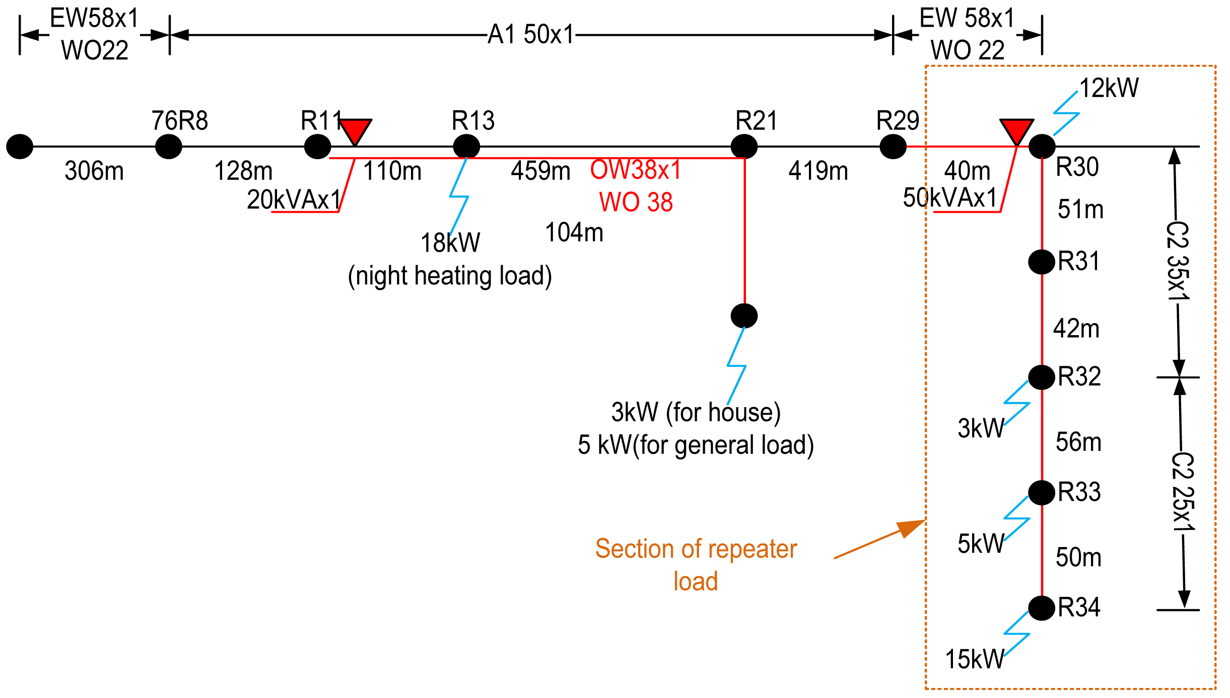
This paper shows the economical evaluation of the LVDC distribution network for communication repeaters in two different cases. The first case is that all sections of the LVDC distribution system consist of O/H lines and the other case is a system with U/G cable. This distribution system has five customers of a communication repeater in a mountainous area where the total power demand is 35 kW and the total distance of the line is approximately 1600 m. Figure 1 shows detailed data of the selected applicable realistic 22.9 kV distribution network for communication repeaters.

In this low voltage system, the distribution voltage is 1500 V (case of bipolar ±750 V) which differs from the 22.9 kV distribution voltage of a normal MVAC system. There are five items to consider for economic feasibility evaluation:

• investment costs;

• energy loss costs;

• interruption and outage costs;

• fault repair costs;

• maintenance costs.

Table 1. Net present value (NPV) analysis parameters. O/H: overhead; U/G: underground; and LVDC: low-voltage direct current.

Parameters	Values	Units
Exchange rate (3 January 2013)	1,423.280	Korean Won (KRW)/€
Average power factor of loads	0.93	pF
Average electricity purchase cost (in 2012)	93.75	KRW/kW h
Average efficiency of power converters	97	%
Lifetime of transformers	30	years
Lifetime of power converters	15	years
Corporate tax rate (CTR)	22	%/year
Failure rate of MVAC O/H line [3]	0.0750	time/km/year
Failure rate of MVAC U/G cable [3]	0.0275	time/km/year
Failure rate of LVDC O/H line [3]	0.0510	time/km/year
Failure rate of LVDC U/G cable [3]	0.0187	time/km/year
Fault repair cost of O/H line [3]	1,423,280	KRW/fault
Fault repair cost of MVAC U/G network [4]	2,334,179.2	KRW/fault
Fault repair cost of LVDC U/G network [4]	2,277,248.0	KRW/fault
Inspection cost of pole transformer (for O/H line) [3]	35,439.672	KRW/unit/year
Inspection cost of pad Transformer (for U/G cable) [3]	39,552.951	KRW/unit/year
Inspection cost of power converter [3]	56,931.200	KRW/unit/year
Maintenance cost of MVAC O/H line	512,000	KRW/km/year
Maintenance cost of MVAC U/G cable	2,886,000	KRW/km/year
Maintenance cost of LVDC O/H line	78,000	KRW/km/year
Maintenance cost of LVDC U/G cable	1,443,000	KRW/km/year

shows the parameters used for NPV analysis [1,2].

2.1.1. Investment Cost

Investment is incurred to remodel the old distribution networks or install new distribution networks. It is computed as follows:

$$C_{\text{inv}}=\sum [(C_{\text{eqip}}+C_{\text{inst}})\times N_{\text{eqip}}]$$

(1)

where C_inv: investment cost; C_eqip: unit price of equipment; C_inst: installation fee; and N_eqip: quantity of equipment.

Various equipments must be considered in any calculation of the investment costs. The first is the transformer; its installation cost is shown in

Table 2. Transformer and power converter installation costs. AC: alternative current; and DC: direct current.

Component	Number	Unit price (KRW)	Installation price(KRW)	Unit sub-total (KRW)
Transformer 50 kVA (one-phase, for MVAC and LVDC)	1	1,113,000	633,333	1,746,333
Rectifier (35 kVA, AC/DC Converter)	1	10,500,000	1,050,000	11,550,000
Inverter (12 kVA, DC/AC Converter)	1	3,600,000	360,000	3,960,000
Inverter (3 kVA, DC/AC Converter)	1	900,000	90,000	990,000
Inverter (5 kVA, DC/AC Converter)	1	1,500,000	150,000	1,650,000
Inverter (15 kVA, DC/AC Converter)	1	4,500,000	450,000	4,950,000

. Replacement cost of power electronic devices considering NPV can be computed with total cost of the converter installation from Table 2 and life-span of devices and real interest rate from Table 1. This can be calculated as follows:

$$C_{\text{CR}}=\frac{C_{\text{CI}}}{(1+{(IR)}^{Y_{\text{CL}}}}=\frac{23,100,000}{1+{0.07}^{15}}=8,372,503\text{KRW}$$

(2)

where C_CR: replacement cost of converter; C_CI: total cost of converter installation; IR: interest rate; and Y_CL: life-span of converter.

The cost of line material and installation should also be considered.

Table 3. Line material and installation costs of MVAC. EW: equipment wire; ABC: aerial bundled cable; and CV: XLPE insulated PVC sheathed cable.

Component	Length (m)	Line installation cost (Including line, 16 m electric pole price) (KRW/m, two-wire)	O/H line cost (KRW)
EW 58 mm2 O/H Line	345	36,761	12,682,545
ABC 50 mm2 O/H Line	1116	64,693	72,197,388
CV 35 mm2 O/H Line	93	33,217	3,089,181
CV 25 mm2 O/H Line	106	30,823	3,267,238

and

Table 4. Line material and installation costs of LVDC.

Line type	Component	Length (m)	Line installation cost (including line cost) (KRW/m)	Total O/H system cost [bipole] (KRW)	Total O/H system cost [monopole] (KRW)
O/H line	OW 60 (three-wire)	1660	35,895	59,585,700	-
	OW 60 (two-wire)	1660	33,988	-	56,420,080
U/G cable	600 V CV 70	1660	52,554	87,239,640	58,159,760

explain the costs of line material and installation of the MVAC network system operating currently and the LVDC system, respectively. The information in these Tables was obtained from the historical database of KEPCO. The total investment cost of the existing MVAC system is 92,982,685 KRW.

In the LVDC O/H line case, the system uses OW 60 mm² and the bipole case has three-wire, while the monopole case has two-wire. In the LVDC U/G cable case, it is replaced to 600 V XLPE insulated PVC sheathed cable (CV) 70 mm² and monopole line installation cost is calculated by 2/3 that of the bipole case.

In conclusion, total investment costs of LVDC system with O/H line is 92,804,536 KRW in bipole case, 89,638,916 KRW in monopole case as following equation and the system with U/G cable is 120,458,476 KRW in bipole case, 91,378,596 KRW in monopole case.

2.1.2. Energy Loss Cost

Energy loss leads to generating wasted electrical power, and this can be converted to the costs. These are caused by line resistance and power converter efficiency. Energy loss of DC distribution line and DC/AC converters are computed with MATLAB/Simulink and conversion efficiency of AC/DC converter is assumed to be 97% which is a common figure. Total energy loss of LVDC network, P_tot is derived by:

$$P_{\text{tot}}=P_{\text{L}}+P_{\text{conv}}$$

(3)

where P_L: energy loss of distribution line; and P_conv: energy loss of DC/AC and AC/DC converters.

The results of energy loss cost of the MVAC and LVDC are shown in

Table 5. Energy loss costs of MVAC and LVDC.

Line type	Total energy loss by simulation (kW)	Year (h)	Average energy price paid by KEPCO (KRW/kW h)	Total loss cost (KRW)
MVAC line	1.5531	8760	93.75	1,275,483
LVDC O/H line	5.6779	8760	93.75	4,662,975
LVDC U/G cable	5.2185			4,285,693

. The rated voltage of LVDC is ±750 V, which needs much larger current for transmitting the same electricity compared to the 22.9 kV MVAC line. The loss of the distribution line is obtained by the following equation:

$$P_{\text{L}}=I^2+R_{\text{L}}$$

(4)

where I: the current of distribution line; and R_L: the resistance of distribution line.

The total energy loss cost is calculated by multiplying the annual average electricity price and the annual energy loss of a distribution network. As a result, the energy loss cost of the LVDC is 3.36–3.66 times greater than that of the MVAC.

2.1.3. Maintenance Cost

The maintenance cost for the distribution system is the sum of the power converter or pole transformer inspection cost and line maintenance cost. This study uses the inspection and maintenance cost data from the KEPCO database to calculate the maintenance cost. In the case of the LVDC, it is not affected by the number of wires in the line, meaning that the maintenance costs of the bipole case and monopole case are the same.

Table 6. Maintenance costs of MVAC.

Component	Number (unit)/length (km-three phase)	Cost (KRW/unit or KRW/km)	Sub-total (KRW)
Pole transformer inspection cost	5.000	35,440	177,198
MVAC O/H line planned maintenance cost	1.461	512,000	748,032
LVAC O/H line planned maintenance cost	0.199	78,000	15,522
Total cost			940,752

shows the maintenance cost of the MVAC network, and

Table 7. Maintenance costs of LVDC.

Component	Number (unit)/length (km-P.N. line)	Cost (KRW/unit)	Sub-total (KRW)
Power converter inspection cost	5.000	56,931	[A] 284,656
LVDC O/H line maintenance cost	1.660	78,000	[B] 129,480
LVDC U/G line maintenance cost	1.660	1,443,000	[C] 2,395,380
Total cost of the O/H Line: [A] + [B] = 414,136
Total cost of the U/G Line: [A] + [C] = 2,680,036

shows the maintenance cost of the LVDC O/H and U/G line.

2.1.4. Fault Repair Cost

The fault repair cost is calculated with the failure rate, line length, line type, and repair cost per fault.

Table 8. Fault repair costs of MVAC.

Component	Failure rate (fault/km/line)	Length (km) × number of lines	Cost (KRW/fault)	Total cost (KRW)
MV O/H line fault repair cost	0.0750	3.32	1,423,280	354,397

and

Table 9. Fault repair costs of LVDC.

Component	Failure rate (fault/km/line)	Length (km) × number of lines	Cost (KRW/fault)	Total (KRW)
LV O/H line fault repair cost (bipole)	0.0510	1.66 × 3 = 4.98	1,423,280	361,485
LV O/H line fault repair cost (monopole)	-	1.66 × 2 = 3.32	-	240,990
LV U/G cable fault repair cost (bipole)	0.0187	1.66 × 3 = 4.98	2,277,248	212,071
LV U/G cable fault repair cost (monopole)	-	1.66 × 2 = 3.32	-	141,381

present the calculations of the fault repair costs of MVAC and LVDC systems, respectively:

$$C_{\text{FR}}=N_{\text{fault}}\times L\times C_{\text{AFR}}$$

(5)

where C_FR: fault repair cost; N_fault: number of fault per km; L: length of distribution line; and C_AFR: average repair cost per fault.

2.1.5. Interruption and Outage Cost [5–9]

Power interruption and outage cost indicates losses of power not delivered to customers as an expense when power interruption occurs. Total power interruption and outage cost (C_POC) is derived by:

$$C_{\text{poc}}=C_{\text{NDE}}+C_{\text{ARC}}=\sum _{j\in J}\{{\lambda }_{\text{com}}\times (a_j+b_j\times t_{\text{rep}})\times P_j\times n_j\}+\sum _{k\in K}\{({\omega }_{\text{kfar}}\times a_{\text{ifar}}+{\omega }_{\text{kdar}}\times a_{\text{idar}})\times P_k\times n_k\}$$

(6)

where C_NDE: annual cost from the non-delivered energy; C_ARC: annual cost of auto-reclosing; a_j: power outage cost parameter for the power not supplied to the load section or customer group j (KRW/kW) [8]; b_j: time dependent power outage per unit cost constant parameter for the energy not supplied to the load section or customer group j (KRW/kW h) [8]; a_ifar: cost parameter of a fast auto-reclosing unit for power not supplied to load section (KRW/kW); a_idar: cost parameter of a time-dependent delayed auto-reclosing unit for energy not supplied to load section (KRW/kW); t_rep: fault repair time for the network component and return of electricity supply; P_j: average yearly power for load section j/customer of group j; n_j and n_k: the number of load sections j and load sections k; ω_kfar: sum of the individual distribution network fast auto reclose fault frequency per year in section k; ω_kdar: sum of the individual distribution network delayed auto reclose fault frequency per year in section k; and P_k: average yearly power for load section in zone k.

The annual cost resulting from non-delivered energy is estimated using the failure/fault rate of the network components and the interruption parameter constants. The interruption parameters used in the calculation are obtained based on the interruption data statistics of residential customers in Korea. The average failure rate of the power electronics converters is 0.3 faults per year/100 units, and that for the pole-mounted transformers is 0.5 faults per year/100 units, with fault repair time, t_rep [9,10].

When estimating the total power outage cost for the LVDC distribution system, the fast automatic reclosing is assumed to be zero. This is due to the fact that the capacitors in the LVDC link can still supply power to residential customers during the short time duration of interruptions prior to the system's restoration to normal operation conditions.

Table 10. Interruption and outage costs of MVAC.

Distribution system type	Permanent fault outage constant parameters		Failure rate of components (λ)	Total time of repair and power restoration (h)	Total feeder load (kW)	Non-delivered energy cost (KRW)
	aj (KRW/kW)	bj (KRW/kW h)
O/H line	4896.96	48,969.6	0.5	6	35	5,227,505
Distribution system type	Incipient interruption constant parameters		Frequency of interruptions (ω_far)	Frequency of interruptions (ω_dar)	Total feeder load (kW)	Auto-reclose cost (KRW)
	aifar (KRW/kW)	aidar (KRW/kW)
O/H line	1.7	2.74	0.7422	0.1295	35	56.58

and

Table 11. Interruption and outage costs of LVDC.

Connection type	Permanent fault outage constant parameters		Failure rate of components (λ)	Total time of repair & power restoration (h)	Total feeder load (kW)	Non-delivered energy cost (KRW)
	aj (KRW/kW)	bj (KRW/kW h)
Bipole	4896.96	48,969.6	0.2	3	35	1,062,640
Monopole	4896.96	48,969.6	0.3	3	35	1,593,960
Distribution system type	Incipient interruption constant parameters		Frequency of interruptions (ω_far)	Frequency of interruptions (ω_dar)	Total feeder load (kW)	Auto-reclose cost (KRW)
	aifar (KRW/kW)	aidar (KRW/kW)
O/H line	1.7	2.74	0	0.1295	35	12.42
U/G cable	1.7	2.74	0	0.0180	35	1.73

present the result of a comparison between the interruption and outage cost of MVAC and LVDC networks. The LVDC line voltage level is much lower than that of the MVAC, therefore, the frequency of supply discontinuance of the LVDC due to contact with the tree is much lower than that of the MVAC, and consequently, the interruption and outage cost of LVDC is highly reduced. As shown on Table 10, the annual interruption and outage cost of existing MVAC distribution line is calculated at 5,227,561 KRW. Then the costs of LVDC O/H line case are able to be calculated at 1,062,652 KRW (bipole) and 1,593,972 KRW (monopole), then in the LVDC U/G cable case, cost is 1,062,642 KRW (bipole) and 1,593,962 KRW (monopole) as shown in Table 11.

2.2. NPV Analysis

This paper performs economic analysis with NPV analysis. The NPV analysis method can express the present monetary value for all calculated costs and is given as:

$$\text{NPV}=C_{\text{inv}}+\mathit{\text{AIR}}\times [\mathit{\text{EBITDA}}\times (1-\mathit{\text{CTR}})-\mathit{\text{DPC}}\times \mathit{\text{CTR}}]$$

(7)

where AIR: annual installation rate of present value; EBITDA: earnings before interest, taxes, depreciation and amortization; CTR: corporate tax rate; and DPC: depreciation cost.

Table 12. NPV evaluation factors.

Factor	Contents
EBITDA	where EBITDA means operation and maintenance (O&M) cost
CTR	where CTR is 22%
DPC	DPC = Cinv/YNPV, where YNPV is year of NPV analysis (30 years)
AIR	AIR = [1−(1+IR)−YNPV]/IR = [1−(1.07)−30]/0.07=12.4 where interest rate (IR) is 7%

shows the factors of NPV evaluation.

Table 13. NPV analysis for first year.

Category	MVAC system	O/H line system		U/G line system
		Bipole	Monopole	Bipole	Monopole
1. Installation Cost	92,982,685	92,804,536	89,638,916	120,458,476	91,378,596
2. Energy Loss Cost	1,275,483	4,662,975	4,662,975	4,285,693	4,285,693
3. Maintenance Cost	940,752	414,136	414,136	2,680,036	2,680,036
4. Fault Repair Cost	354,397	361,485	240,990	212,071	141,381
5. Power Outage Cost	5,227,561	1,062,653	1,593,973	1,062,642	1,593,962
Total Cost	100,780,879	99,305,785	96,550,990	128,698,919	100,079,668

expresses the result of economic feasibility evaluation considering NPV for the first year after installation compared to the O/H line system and U/G cable system.

Table 14. NPV analysis for 30 years (KRW).

Category	MVAC system	O/H line system		U/G cable system
		Bipole	Monopole	Bipole	Monopole
Investment Cost	92,982,685	92,804,536	89,638,916	120,458,476	91,378,596
Annual O&M Cost (EBITDA)	7,798,194	6,501,249	6,912,074	8,240,442	8,701,072
EBITDA × (1 − CTR)	6,082,591	5,070,974	5,391,418	6,427,545	6,786,836
Depreciation cost (DPC) for 30 years	3,099,423	3,093,485	2,987,964	4,015,283	3,045,953
DPC × CTR	681,873	680,567	657,352	883,362	670,110
EBITDA × (1 − CTR) − DPC × CTR	5,400,718	4,390,407	4,734,066	5,544,183	6,116,726
Annual Installation Rate of Present Value (AIR)	12.41	12.41	12.41	12.41	12.41
O&M Cost (NPV)	67,017,734	54,480,747	58,745,216	68,797,992	75,902,710
Overall NPV	160,000,419	147,285,283	148,384,133	189,256,468	167,281,307

shows the result of NPV analysis for 30 years and verifies that the most economical method to install a distribution line for communication repeaters is the LVDC bipolar overhead system. The overall NPV costs of bipolar and monopolar LVDC distribution networks of U/G cable are higher than for the O/H line system by approximately 28% and 12%, respectively, and the cost of the MVAC network is approximately in between those of the LVDC O/H line and U/G cable.

In consideration of replacing MVAC with LVDC, the O/H line configuration is an economical solution, and the NPV cost of the U/G cable is not much higher than the cost of MVAC. Therefore, if U/G cable were considered for a low loaded distribution line due to environmental or security reasons, the LVDC underground network is a reasonable solution regarding economic aspects.

3. LVDC Testbed and Simulation Model

KEPCO simultaneously conducts installation of the LVDC distribution testbed in KEPRI and development of the simulation model with PSCAD/EMTDC [11] to conduct various tests and analyses of the LVDC distribution line.

3.1. Configuration of the LVDC Testbed

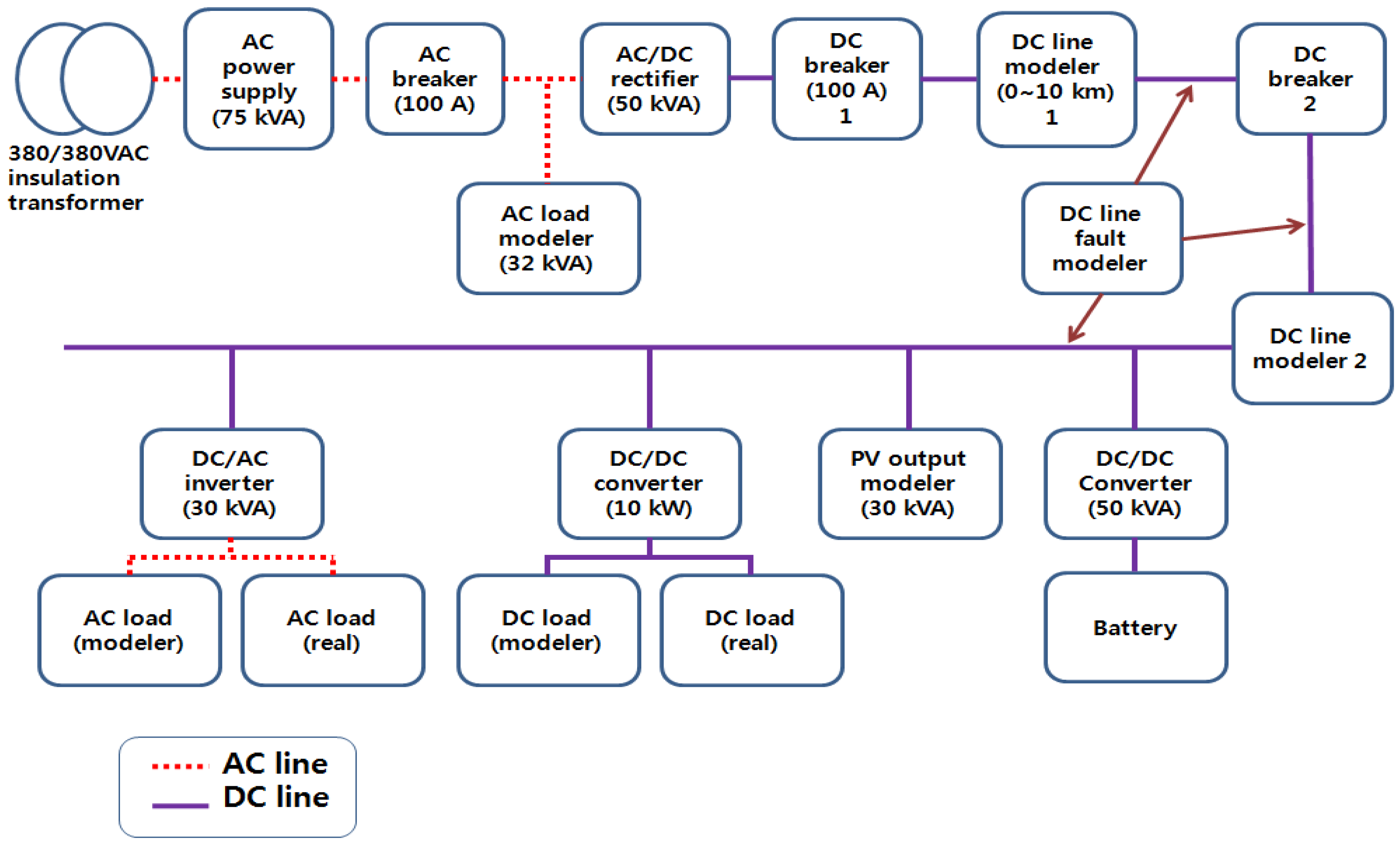
Figures 2 and 3 shows the overall schematic diagram of the LVDC testbed of KEPCO and its simulation model, respectively. The objective of the LVDC testbed is to test developed power conversion systems for LVDC, failure effects analysis on DC lines, determining the possible distribution line length with DC lines, connection test with decentralized power supply system and so on. This testbed is able to operate in bipole ±750 V and ±380 V or monopole 380 V, 750 V and 1500 V [12]. Thus, it can be utilized as the test infrastructure for further various LVDC distribution and micro-grid tests.

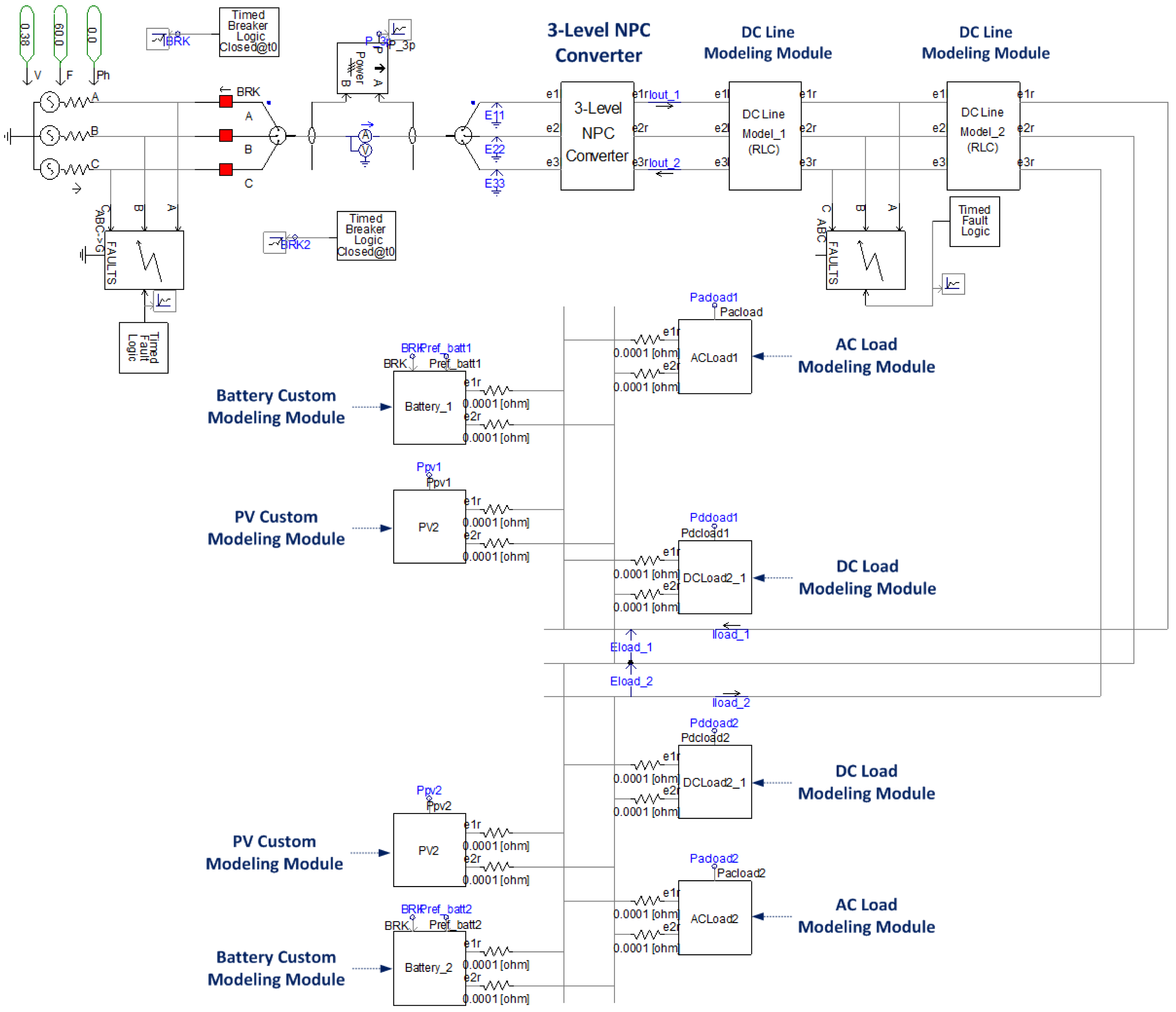
3.2. Simulation Model

The simulation model of the LVDC testbed has been developed with PSCAD/EMTDC. Pre-simulation will be performed with this simulation model before conducting hardware tests and cross-verification between the result of hardware and software tests. The rectifier is three-level Neutral-Point-Clamped (NPC) converter which is powered by a 60 Hz three-phase 380 V AC network. This converter outputs bipole DC power and DC line is consist of two models to simulate the fault occur at middle point of DC line. In case of models of battery, photovoltaic (PV) generator and AC and DC load, models for positive pole and negative pole exist, respectively.

3.2.1. AC/DC Converter Model

The AC/DC converter being developed for the testbed is selected as a three-level NPC converter [12,13] consisting of 12 IGBTs and 6 diodes. This converter has lower voltage fluctuation range. Thus, it incurs less dV/dt stress than a conservative two-level pulse width modulation (PWM) converter. Although a three-level converter consists of a number of devices, the voltage ratings of semiconductor switching devices are able to be half the voltage ratings of a two-level converter.

3.2.2. DC Load Model

The developed DC load model, consisting of a buck converter, converts a voltage level from DC distribution lines to a lower voltage for DC loads. For the scheduling function, a scheduled power consumption is input through a load scheduling file (*.list) and changed as R load through the equation, R = V²/P.

3.2.3. AC Load Model

The developed AC load model consists of a three-phase two-level inverter, getting scheduled power by a linked scheduling file, as for the DC load model.

3.2.4. PV Generator Model

The PV model for the testbed basically outputs the scheduled PV output with a constant voltage characteristic, not featured with Maximum Power Point Tracking (MPPT) control, PV cell characteristic, etc., like a real PV system. It consists of a boost converter that converts the voltage level from PV cell to the level of DC distribution lines.

3.2.5. Battery Model

The battery model for the testbed outputs the calculated power as an uninterruptable power supply (UPS) device when fault occurs on the AC side. MPPT control, PV cell characteristic, state of charge (SOC) estimation by battery management system (BMS), etc. are not considered. When a fault occurs, the battery output reference is calculated using the following equation:

$$P_{\text{batt}(\text{ref})}=(P_{\text{dc},\text{load}}+P_{\text{ac},\text{load}})-P_{\text{pv},\text{out}}$$

(8)

where P_batt(ref): reference of the battery system; P_dc,load: kW of DC load; P_ac,load: kW of AC load; and P_pv,out: kW output of PV.

4. Simulation Study

In this section, dynamic characteristic analysis is performed when the LVDC distribution line for communication repeaters is installed with an O/H line or U/G cable. For this analysis, the line constant is first computed for the U/G cable and O/H line 1600 m long. Then the difference in the fault voltage and current is analyzed by the PSCAD/EMTDC simulation study using the computed line constant.

4.1. Computation of Line Parameters

4.1.1. Line Parameters of U/G Cable

The U/G cable of the DC distribution line for the simulation study is 70 mm², 0.6/1 kV, three-core CV cable. Resistance, inductance and capacitance of this cable are 0.268 Ω/km, 0.013 mH/km and 0.657 uF/km, respectively. Since cable manufacturers have their own production methods, the public company is not able to know the line parameters. The best way to obtain accurate parameters is through the manufacturer. The data mentioned above are measured parameters provided by the manufacturer, JS Cable Inc. (Choongnam, Korea).

4.1.2. Line Parameters of O/H Line [9]

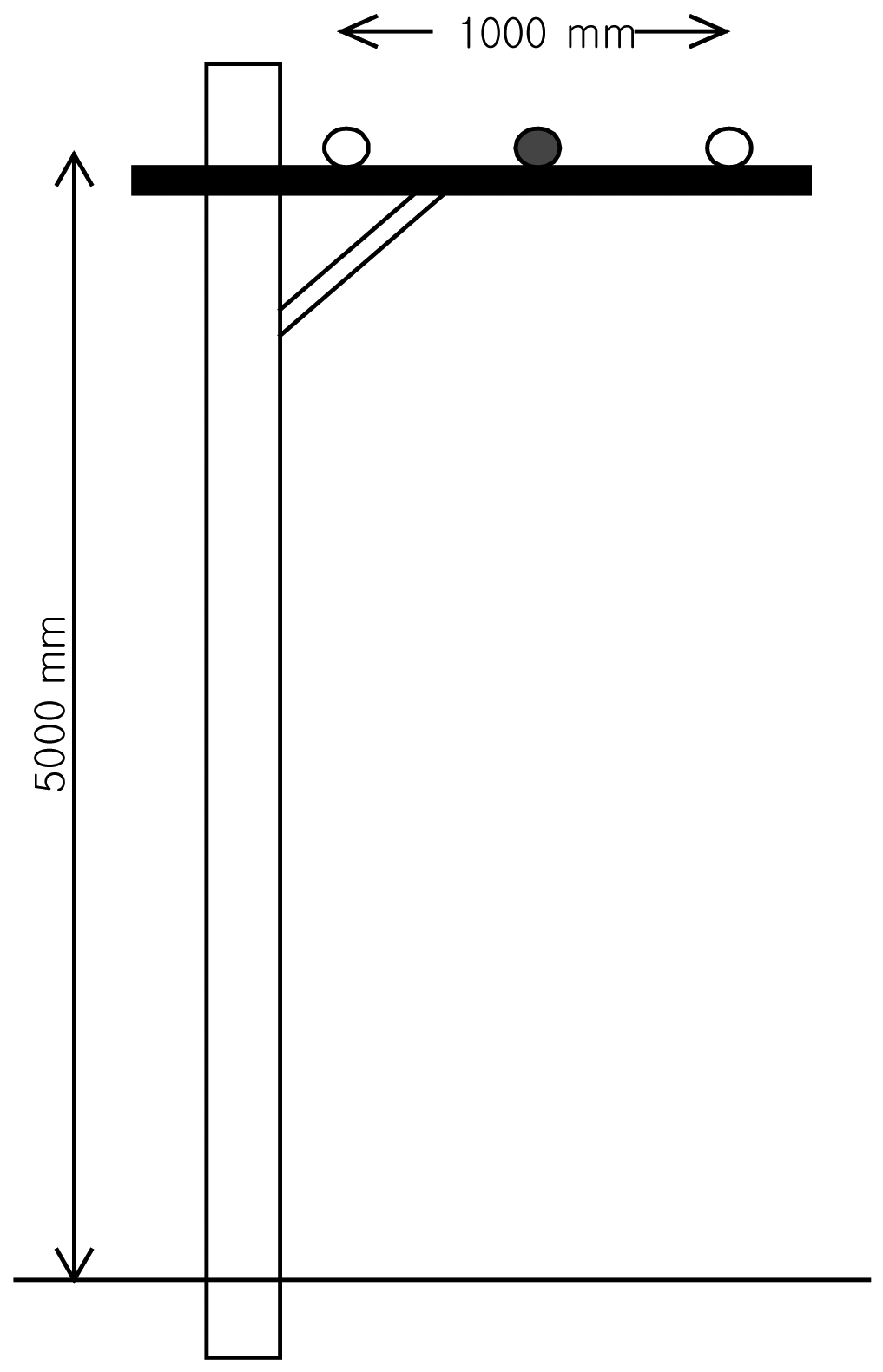
The O/H line of the DC distribution line for the simulation study is an outdoor weather-proof polyvinyl chloride insulated (OW) wire with a 60 mm² cross section. In the case of the O/H line, line parameters are affected by the configuration of the O/H line. In general, parameters of an O/H line have much bigger inductance and much smaller capacitance, because the distance of the conductors is very far for the case of a U/G cable. Figure 4 expresses the configuration of the O/H line presumed for computing the line parameters. Where, distances between wires are identical and the colored wire is a neutral line. The conductor of 60 mm² OW wire is annealed copper wire of 4.37 mm radius.

The resistivity of this conductor can be derived as follows:

$$\rho =\frac{1}{58}\times \frac{100}{C_{\text{p}}}=0.017$$

(9)

where C_p : conductivity (100, annealed copper wire).

Resistance can be determined by:

$$R=\rho \times \left(\frac{1}{A}\right)=0.017\times \left(\frac{1}{60}\right)=0.46\Omega /km$$

(10)

where A: cross-section (=60 mm²).

Inductance of the O/H line can be derived as follows:

$$L=L_1+L_2=0.921log\frac{D}{r^{\text{'}}}=2.273\text{mH}/\text{km}$$

(11)

where r′: radius of fictitious conductor (=0.7788r); and D: distance between conductors of ±pole (=1000 mm).

Thus, L₁ and L₂ are equally to 1.137 mH/km.

Line-to-line capacitance, C_ab can be derived by:

$$C_{\text{ab}}=\frac{0.0121}{log\left(\frac{D}{r}\right)}=5.122\times {10}^{-3}\mu \text{F}/\text{km}$$

(12)

Line-to-neutral capacitance, C_an and C_bn can be derived by:

$$C_{\text{an}}=C_{\text{bn}}=2C_{\text{ab}}=\frac{0.0242}{log\left(\frac{D}{r}\right)}=10.24\times {10}^{-3}\mu \text{F}/\text{km}$$

(13)

4.2. Simulation Study

The parameters of the DC line obtained above are modeled by two T-equivalent RLC circuits to analyze the fault in the middle of the DC line. The

Table 15. Comparison of line parameters of 1.6 km LVDC distribution line.

Type	O/H line	U/G cable	Unit
Resistance	0.736	0.4288	Ω
Inductance	1.8192	0.0208	mH
Capacitance	0.082 (Line-to-line) 0.0164 (Line-to-neutral)	1.0512	μF

expresses the parameter differences between U/G cable and O/H line with a line length of 1.6 km.

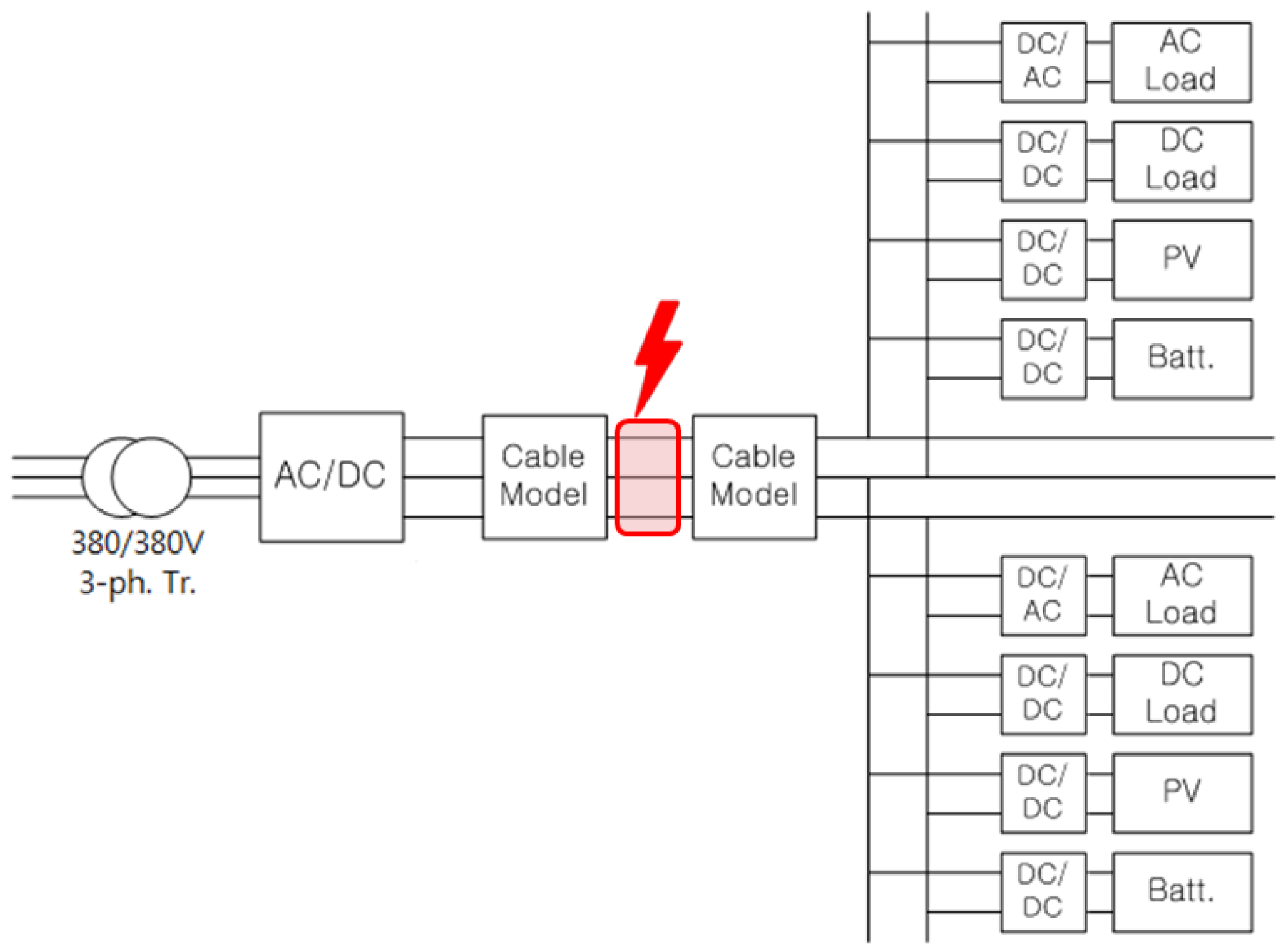
As shown on Table 15, there is considerable difference between the parameters of U/G cable and O/H line. This simulation study deals with the differences of fault current and voltage when a DC line fault occurs. A three-line short is the most serious fault that can occur on a DC distribution line. When a fault occurs, if the fault current is bigger, the connected devices might get a bigger shock and it is necessary to enlarge the capacity of the associated circuit breakers. Figure 5 depicts the overall schematic diagram of the LVDC testbed model and fault point.

PV generators respectively output 5 kW and batteries are not operated to analyze just the short-circuit current of the DC line fault. The point of fault occurrence is in the middle of the 1.6 km DC distribution line and the duration time is 50 ms (0.6–0.65 s).

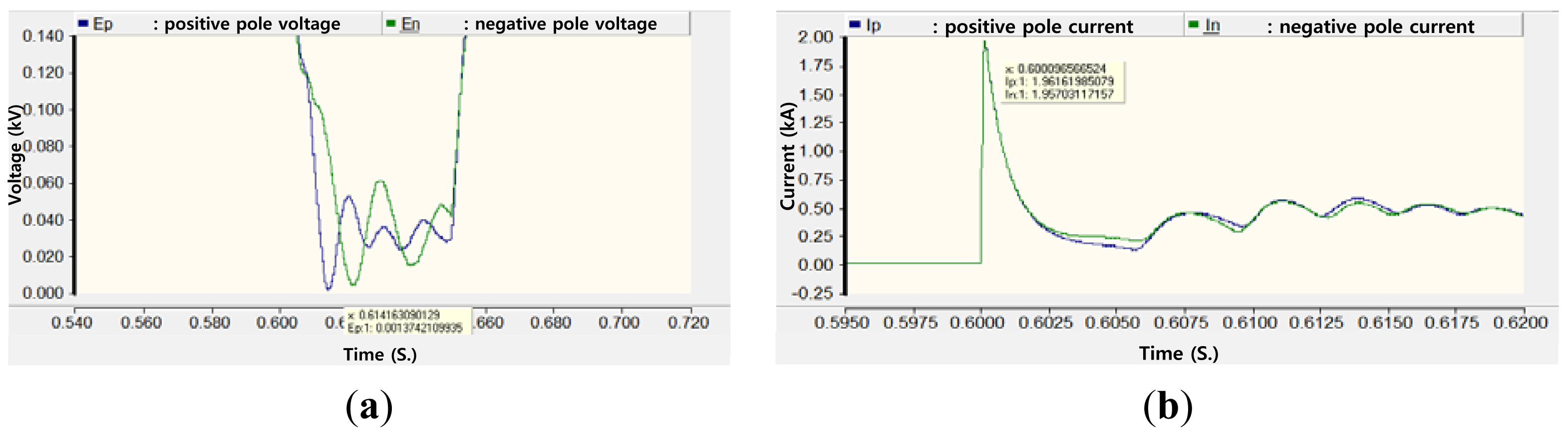
4.2.1. Fault Case of U/G Cable

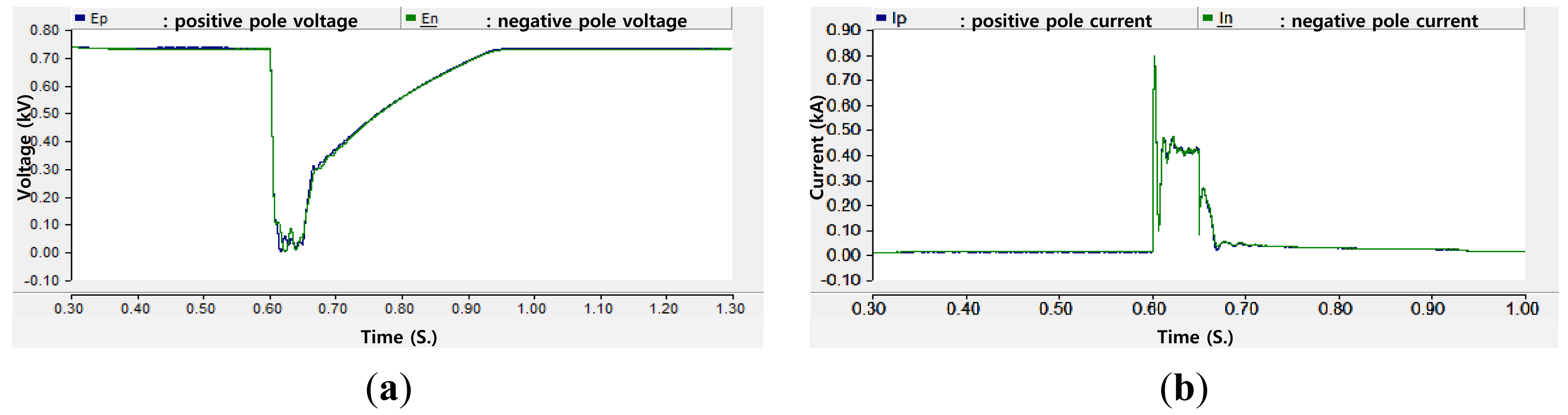
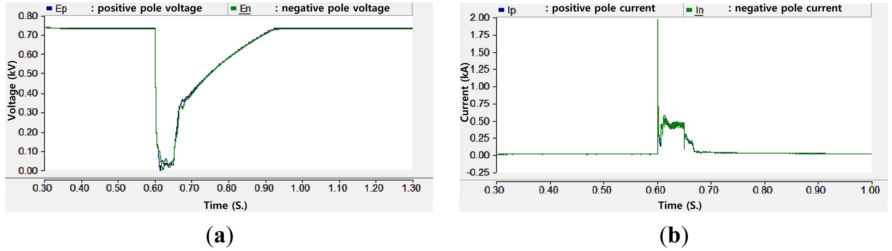
Figures 6 and 7 show the result of a three-line short fault in a U/G cable line. After a fault occurs, the voltage levels of the bipolar DC line decrease to zero drastically; after relieving the fault at 0.65 s, the DC line recovers the nominal voltage level gradually. The maximum fault current level is 1956 A and waveforms of bipolar currents are almost the same.

4.2.2. Fault Case of O/H Line

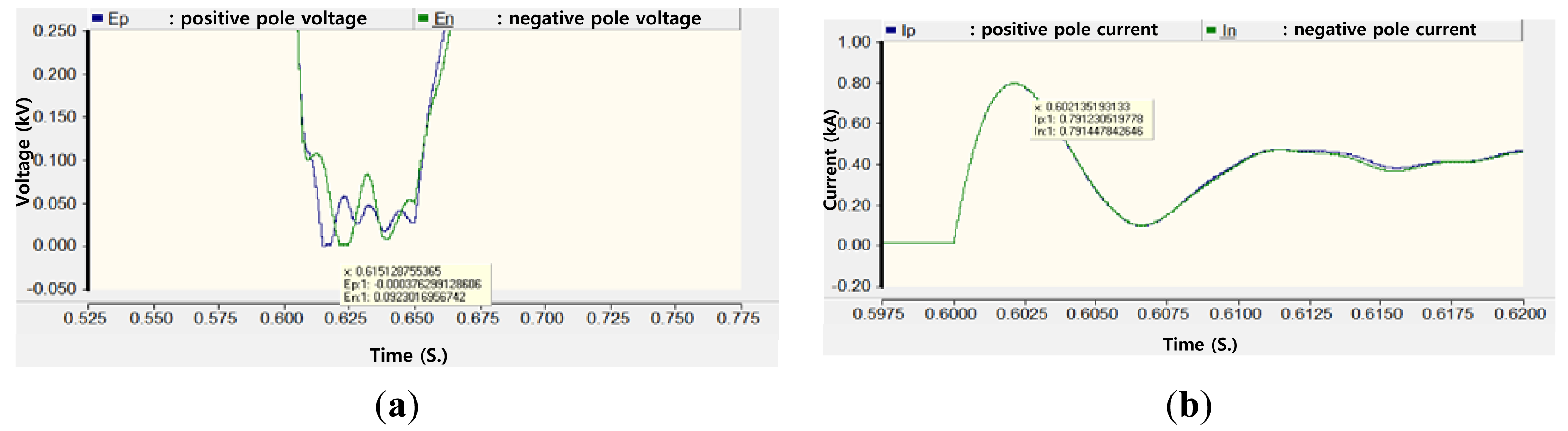
Figures 8 and 9 show the results of an O/H line fault. The trend of fault voltage is similar as the above case and the maximum current levels are 0.791, 0.4 times the result of the above case. Thus, the difference of line parameters causes considerable differences in fault current and additional expense might be needed to increase the capacity of the circuit breakers and other devices when the LVDC distribution line is installed with U/G cable.

5. Conclusions

KEPRI is researching the business models of the LVDC distribution and distribution network for communication repeaters as one of LVDC business models. This paper analyzed the difference between U/G cable and O/H line for a LVDC distribution line for communication repeaters in a mountainous area. For analysis, a realistic applicable MVAC distribution line was selected and an economic feasibility evaluation for each type of distribution line was conducted. The result showed that the overall NPV cost for 30 years with a U/G cable is approximately 12% to 28% higher, depending on the configuration than the cost with O/H lines, and the NPV cost of the existing MVAC system is approximately between the results of LVDC U/G cable and O/H line configurations.

Then the LVDC testbed being installed was explained. It consists of an AC/DC converter, simulators of a PV generator, AC load, DC load, DC distribution line and DC line fault, battery and so on. The objectives of the LVDC testbed are various hardware tests for the LVDC distribution and DC microgrid. In addition, a PSCAD/EMTDC model of the testbed was developed to perform pre-simulation and cross-verification between results of hardware and software tests.

Simulation studies were conducted to compare the fault simulation results of U/G cable and O/H line for the LVDC distribution network. The results verified that the fault current level in the case of an O/H line is significantly less than the fault current level in the case of U/G cable. Results of economic feasibility evaluation and dynamic characteristic analysis with PSCAD/EMTDC would be utilized to select an appropriate type of LVDC distribution line.

References

- Hur, D. Economic Considerations Underlying the Adoption of HVDC and HVAC for the Connection of an Offshore Wind Farm in Korea. J. Electr. Eng. Technol. 2012, 7, 157–162. [Google Scholar]
- Lassila, J.; Kaipia, T.; Partanen, J.; Järventausta, P.; Verho, P.; Mäkinen, A.; Kivikko, K.; Lohjala, J. A Comparison of the Electricity Distribution Investment Strategies. Proceedings of the 19th International Conference on Electricity Distribution, Vienna, Austria, 21–24 May 2007.
- Naakka, V. Reliability and Economy Analysis of the LVDC Distribution System. Master's Thesis, Tampere University of Technology, Tampere, Finland, December 2011. [Google Scholar]
- Kaipia, T.; Salonen, P.; Lassila, J.; Partanen, J. Possibilities of the Low Voltage DC Distribution Systems. Proceedings of the Nordac, Nordic Distribution and Asset Management Conference, Stockholm, Sweden, 21–22 August 2006.
- Kivikko, K.; Makinen, A.; Verho, P.; Jarventausta, P. Outage Cost Modelling for Reliability Based Network Planning and Regulation of Distribution Companies. Proceedings of the 8th IEE International Conference on Developments in Power System Protection, Amsterdam, The Netherlands, 5–8 April 2004; Volume 2, pp. 607–610.
- Lassila, J.; Honkapuro, S.; Partanen, J. Economic Analysis of Outage Costs Parameters and Their Implications on Investment Decisions. Proceedings of the IEEE Power Engineering Society General Meeting, San Francisco, CA, USA, 12–16 June 2005.
- Lagland, H. Comparison of Different Reliability Improving Investment Strategies of Finnish Medium-Voltage Distribution Systems. Acta Wasaensia 2012, 42, 1–216. [Google Scholar]
- Bozic, Z. Customer Interruption Cost Calculation for Reliability Economics: Practical Considerations. Proceedings of the International Conference on Power System Technology, Perth, Australia, 4–7 December 2000; Volume 2, pp. 1095–1100.
- Roos, F.; Lindahl, S. Distribution System Component Failure Rates and Repair Times—An Overview. Proceedings of the Nordic Distribution and Asset Management Conference, Espoo, Finland, 23–24 August 2004; pp. 1–6.
- Short, T.A. Electrical Power Distribution Handbook; CRC Press: Boca Raton, FL, USA, 2004. [Google Scholar]
- PSCAD/EMTDC User Manual; Manitoba Hydro HVDC Centre: Montreal, QC, Canada, 2010.
- Lago, J.; Moia, J.; Heldwein, M.L. Evaluation of Power Converters to Implement Bipolar DC Active Distribution Networks—DC-DC Converters. Proceedings of the IEEE Energy Conversion Congress and Exposition (ECCE), Phoenix, AZ, USA, 17–22 September 2011; pp. 985–990.
- Pou, J.; Zaragoza, J.; Ceballos, S.; Saeedifard, M.; Boroyevich, D. A Carrier-Based PWM Strategy with Zero-Sequence Voltage Injection for a Three-Level Neutral-Point-Clamped Converter. IEEE Trans. Power Electron. 2012, 27, 642–651. [Google Scholar]