Optimal Sizing and Control of Battery Energy Storage System for Peak Load Shaving

Abstract

Battery Energy Storage System (BESS) can be utilized to shave the peak load in power systems and thus defer the need to upgrade the power grid. Based on a rolling load forecasting method, along with the peak load reduction requirements in reality, at the planning level, we propose a BESS capacity planning model for peak and load shaving problem. At the operational level, we consider the optimal control policy towards charging and discharging power with two different optimization objectives: one is to diminish the difference between the peak load and the valley load, the other is to minimize the daily load variance. Particularly, the constraint of charging and discharging cycles, which is an important issue in practice, is taken into consideration. Finally, based on real load data, we provide simulation results that validate the proposed optimization models and control strategies.

1. Introduction

With the development of the load demands and renewable energy integration, the huge differences between peak and valley loads are pushing the power companies to upgrade the existing power systems. However, the investment may not be economical due to the relative short duration of the peak loads, which leads to an extremely low equipment utilization ratio. The battery energy storage system (BESS), which can supply energy during high demand periods and consume energy in low demand periods, is an advanced alternative to address this challenge [1,2]. From the peak load shaving aspect, the design of the BESS consists of two levels. At the planning level, we need to minimize the power capacity of the BESS while achieving the peak load shaving target. At the operational level, the control policy towards charging and discharging power should be improved so as to optimize the peak load shaving.

For the BESS planning optimization, the accuracy of predicted load curve is important to design the control strategy [3]. Load forecast methods can be broadly divided into two categories: traditional forecast methods (time series method, regression analysis, trend extrapolation, elastic coefficient method, etc.) and artificial intelligence methods (expert systems, fuzzy logic methods, neural network methods, etc.) [4]. The regression analysis method is simple and easy to understand—no off-line training is necessary—and easy to implement [5]. Several load points are predicted using a multi-regression model in [3]. Some load curves that fit to these points are searched and selected from past recorded data to derive a continuous load curve by weighted averaging. The short-term load forecast method presented in this paper not only makes use of the historical load data before the predicted day, as the traditional forecast methods do, but also takes advantage of the obtained data on the predicted day by passage of time. The predicted load curve is used to solve for real time BESS control strategy.

For the operational control strategy, optimization algorithms can also be divided into intelligent algorithms and classical algorithms. Intelligent algorithms are used in [6–8], including particle swarm optimization [6], evolutionary algorithm [7], and simulated annealing [8]. Intelligent algorithms can solve models including discontinuous and nonlinear constraints, but they cannot assure that they converge to the global optimal solution, and their parameters are difficult to choose. Classical algorithms, such as dynamic programming [9,10] and mixed integer programming [11,12], have been employed in the sizing and operation optimization. However, under a forecasting framework, dynamic programming will encounter the “curse of dimensionality”, which is very complicated to solve. For the control strategy, a critical issue is how to manage the charging and discharging process of the BESS in order to maximum the welfare under a limited BESS capacity [13–17]. A static model of BESS is established to minimize the amount and the time of power-off [13]. The paper studies how to improve the power system reliability through peak load shaving with BESS. The study in [15] analyzes the economics of grid level energy storage for the application of load shaving. To be accurate to the real power allocation, charging and discharging rates were modeled for simulation purposes. Similarly, a derived discharging simulation model was developed in [16] for evaluation of the ampere-hour capacity of the battery needed for load shaving. These studies, however, only consider the theoretical constraints in physics but ignore the operational constraints in practice.

In this paper, the mixed-integer programming (MIP) method based on a new BESS model is used, which is different from the typical approaches that merely consider physical constraints of the BESS, since operational constrains are also taken into consideration. Meanwhile, the model is designed to minimize either the load range, or the load variance, or both. In addition, the number of charging and discharging cycles is considered as the constraint to better reflect the usage of BESS instead of the number of charging and discharging. Although this study focuses on the BESS, the proposed methods in this paper can be applied to any kind of energy storage systems.

The remainder of the paper is organized as follows. Optimal sizing model is presented in Section 2. Section 3 introduces the rolling forecasting method. We then establish two models of charging and discharging control process in Section 4. Section 5 presents the simulation results.

2. Optimal Sizing Model

The BESS capacity is measured in two dimensions, i.e., power capacity and energy capacity, respectively. The power capacity is represented by the maximum discharging power and the maximum charging power. The power capacity varies in different scenarios. On the generation side, the power capacity is relevant to the peak load and the capacity of generators. On the transmission and distribution side, however, the power capacity is relevant to the possible maximum load and the transmission capability.

We optimize the energy capacity of the BESS based on the assumption that the power capacity of the system has already been determined. The power output of BESS is positive when discharging, while negative when charging. Let P_cap denote the power capacity of the BESS, thus the maximum discharging power $P_{S,disch}^{max}=P_{cap}$ and the maximum charging power $P_{S,ch}^{max}=-P_{cap}$. Let E_cap denote the energy capacity of the BESS. Since the maximum values of powers are determined, we then optimize the energy capacity of the BESS. The objective function is as follows.

$$minf=E_{cap}$$

(1)

When optimizing the energy capacity, the power output constraints should be satisfied.

$$\begin{array}{l}0\le P_S^{+}(k)\le u_S^{+}(k)·P_{S,disch}^{max}\\ u_S^{-}(k)·P_{S,ch}^{max}\le P_S^{-}(k)\le 0\end{array}$$

(2)

Here $P_S^{+}(k)$ and $P_S^{-}(k)$ represent the discharging power and the charging power of the BESS at time k, respectively, and $u_S^{+}(k)$ and $u_S^{-}(k)$ denote, respectively, the state of discharging and charging of the BESS. Note that $u_S^{+}(k)$ and $u_S^{-}(k)$ have to satisfy

$$\begin{array}{r}{u}_S^{+}(k)+u_S^{-}(k)=1\\ u_S^{+}(k)·\left(u_S^{+}(k)-1\right)=0\\ u_S^{-}(k)·\left(u_S^{-}(k)-1\right)=0\end{array}$$

(3)

If $u_S^{+}(k)=0$ and $u_S^{-}(k)=1$, then the BESS is charging. If $u_S^{+}(k)=1$ and $u_S^{-}(k)=0$, then the BESS is discharging.

In addition to the power constraints, the energy constraints should also be considered. Let E(k) represent the remaining energy of the BESS at time k, with E(0) being the remaining energy at the beginning and E(n) being the remaining energy at the end of the day. In addition, ε_low and ε_high are the lowest and the highest percentage of the remaining energy, respectively. Both ε_low and ε_high range from 0% to 100% with ε_low ≤ ε_high.

$${\epsilon }_{low}{E}_{cap}\le E(k)\le {\epsilon }_{high}{E}_{cap}$$

(4)

To achieve continuous peak load shaving, the remaining energy at the end of the day should be the same as that at the beginning of the day, which is represented by

$$E(n)=E(0)$$

(5)

The relationship between the power output of the BESS and the remaining energy of BESS are shown as follows, with η⁺ being the discharging efficiency, η⁻ being the charging efficiency, and △t being the length of a single time step.

$$E(k+1)=E(k)-(P_S^{+}(k)/{\eta }^{+}+P_S^{-}(k)·{\eta }^{-})·△t$$

(6)

Besides, the peak load shaving constraint should also be satisfied. In such constraint, P_L(k) is the load at time k, while $P_L^{max}$ is the peak load during the time period concerned. The constraint assures that the amount of peak load shaved will match the power capacity P_cap.

$$P_L(k)-P_S^{+}(k)-P_S^{-}(k)\le P_L^{max}-P_{cap}$$

(7)

The above model consisting of all listed formulas is a mixed-integer programming (MIP) optimization model.

The final energy capacity of the BESS is determined as follows. First, based on historical load curves, we evaluate the energy capacity required to accomplish peak load shaving for each day. Among these results, pick an energy capacity that can cover p percentage of the peak load shaving tasks. The p percentage, which ranges from 0% to 100%, is assigned to be the percentage of the mission-completed days under a specified energy capacity and different daily loads.

3. Rolling Load Forecasting Method

Load forecasting is essential to peak load shaving and the forecasting accuracy directly affects the effectiveness of peak load shaving. Short-period forecasting methods include time series analysis, regression analysis, artificial neural network, support vector machine (SVM), among others. Regression analysis is the cornerstone of the rolling load forecasting (RLF) proposed in this study.

When predicting the load through regression analysis, the real loads of early time in the day are needed to obtain the optimal regression parameters, which will be used when predicting the loads in the rest of the day.

We adopt the Mean Average Percentage Error (MAPE) to evaluate the prediction accuracy. The MAPE is calculated as follows.

$$MAPE=\frac{1}{n}{\displaystyle \sum _{i=1}^n\frac{\left|x(i)-\widehat{x}(i)\right|}{x(i)}}$$

(8)

where x(i) and $\widehat{x}$ (i) represent the real value and the predicted value of the target day; and n is the sampling number of the target day.

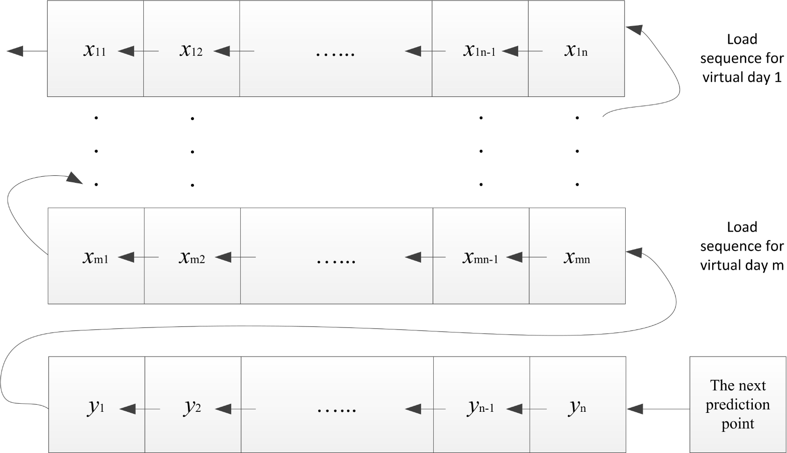
However, the data is far from enough if only early time of the day is considered. With the RLF method we propose, historical load data of the same time in the preceding days are grouped together to make prediction for the present time. We call the time period from present time to the same time in the preceding day as a virtual day.

Considering that the regression parameter we calculate for a certain prediction will not always be optimal, we refresh the regression parameter each time we make a new prediction for the next prediction time. The rolling algorithm is shown as in Figure 1.

On each prediction of y_i (i = 1, 2, …, n), we use the following equation:

$$y_i={\displaystyle \sum _{j=1}^m{r}_{ji}{x}_{ji}}$$

(9)

where for each calculation, the optimal regression parameter r_ji, j = 1, 2, …, m will be updated.

We will only compare our RLF with Average Load Forecasting (ALF), which is widely used in practice. It is noted that RLF is not a novel method in forecasting theory, but we will show that RLF is significantly better than ALF, especially when there are high prediction errors.

4. Charging and Discharging Model

4.1. Minimizing the Gap between Peak and Valley

During the peak load periods, the BESS outputs active power to shave the peak load. During the valley load periods, however, the BESS absorbs the active power from the power system. Denote P_level1 as the load reduction in peak hours and P_level2 as the load compensation in the valley hours. The objective functions can be written as

$$maxf=\alpha P_{level1}+(1-\alpha )P_{level2}$$

(10)

where α ϵ [0,1]. If α is larger than 0.5, the load reduction bears higher weight in the objective, and vice versa. Note that P_level1 and P_level2 have to satisfy

$$\begin{array}{l}0\le P_{level1}\le P_{S,disch}^{max}\\ 0\le P_{level2}\le -P_{S,ch}^{max}\end{array}$$

(11)

$$\begin{array}{l}{P}_L(k)-P_S^{\text{+}}(k)-P_S^{-}(k)\le P_L^{max}-P_{level1}\\ P_L(k)-P_S^{\text{+}}(k)-P_S^{-}(k)\le P_L^{min}-P_{level2}\end{array}$$

(12)

There are also constraints on power, state of charging and discharging as well as energy for the optimization of charging and discharging powers of the storage system. The constraints are shown below.

$$\begin{array}{l}0\le P_S^{\text{+}}(k)\le u_S^{+}(k)·P_{S,disch}^{max}\\ u_S^{-}(k)·P_{S,ch}^{max}\le P_S^{-}(k)\le 0\end{array}$$

(13)

$$\begin{array}{r}{u}_S^{+}(k)+u_S^{-}(k)=1\\ u_S^{+}(k)·\left(u_S^{+}(k)-1\right)=0\\ u_S^{-}(k)·\left(u_S^{-}(k)-1\right)=0\end{array}$$

(14)

$${\epsilon }_{low}{E}_{cap}\le E(k)\le {\epsilon }_{high}{E}_{cap}$$

(15)

$$E(n)=E(0)$$

(16)

$$E(k+1)=E(k)-\left(P_S^{+}(k)/{\eta }^{+}+P_S^{-}(k)·{\eta }^{-}\right)·△t$$

(17)

The more charging and discharging cycles the BESS experiences, the more lifetime reduction of the storage units will incur. If the output of BESS reaches the rated amount of the system energy, a same amount of energy should be absorbed before the next cycle of discharge. Thus, the charging and discharging cycles can be represented by the ratio of the total energy discharged and the energy capacity. For the purpose of system lifecycle extension, the charging and discharging cycles are constrained by

$${\displaystyle \sum _{k=1}^n{P}_S^{+}(k)/{\eta }^{+}}·△t\le c·E_{cap}$$

(18)

where c is the maximum number of the charging and discharging cycles allowed. It is an adjustable constant in the practice of BESS. If c is too small, the BESS will be thoroughly utilized at all times, but the load shaving tasks may still be missed, while if it is too large, the BESS may become underutilized, which can be a waste of the capacity of BESS. There is a threshold for c to achieve the largest amount of load shaving (In model 1, the threshold is 1.28), above which the constraint would lose its power.

4.2. Minimizing the Variance of Daily Load

In the above model, the weighted sum of peak load reduction and the valley load compensation is set to be the objective function. As we can see, the goal of peak load shaving is to iron out peaks and valleys as much as possible, that is, to reduce the fluctuation of the load curve during one-day period. In that case, our objective can be written as to minimize the variance of the load curve, which is

$$f_1=\frac{1}{n}{{\displaystyle \sum _{k=1}^n\left[\left(P_L(k)-P_S^{+}(k)-P_S^{-}(k)\right)-P_L^{mean}\right]}}^2$$

(19)

where $P_L^{mean}$ is the average value of load within a day. To smooth out the curve, an additional item that represents the fluctuation of adjacent time can be written as follows.

$$f_2=\frac{1}{n-1}{{\displaystyle \sum _{i=1}^{n-1}\left[P_L(k+1)-P_S^{+}(k+1)-P_S^{-}(k+1)-P_L(k)+P_S^{+}(k)+P_S^{-}(k)\right]}}^2$$

(20)

The final objective function is shown in Equation 20, where β is the weight of two items in the function, and β ϵ [0, 1]. If β is 1, then only the variance is considered, otherwise, the adjacent-time fluctuation is the also considered.

$$minf=\mathrm{\beta }{f}_1+(1-\mathrm{\beta })f_2$$

(21)

In addition, the second model that we just introduced contains constraints of Conditions 12–17. Extra constraints are raised to ensure the effectiveness of peak load shaving as follows:

$$\begin{array}{l}{P}_L(k)-P_S^{+}(k)-P_S^{-}(k)\le -P_L^{max}-min\left({\gamma }_1{P}_{S,disch}^{max},P_L^{max}-P_L^{mean}\right)\\ P_L(k)-P_S^{+}(k)-P_S^{-}(k)\le -P_L^{min}-min\left({\gamma }_2{P}_{S,ch}^{max},P_L^{mean}-P_L^{min}\right)\end{array}$$

(22)

where γ₁ and γ₂ are between 0 and 1. This is to maximize both the load reduction in peak hours and the load compensation in valley hours.

5. Simulation Results

5.1. Case Description

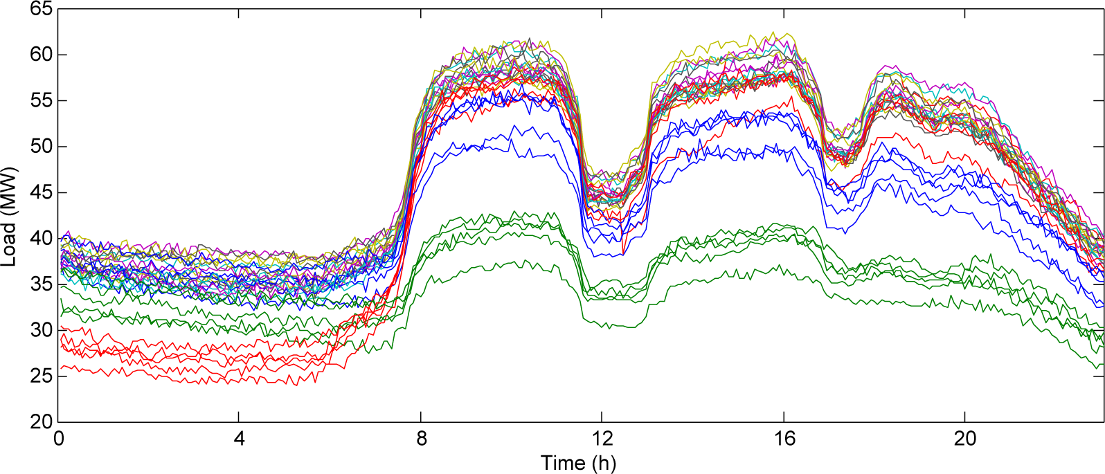
The historical load from the Biling Substation in ShenZhen during the entire March in 2014 is shown in Figure 2. The sample interval is 5 min, thus we have 288 samples per day. There are three peaks in the area, i.e., around 10:00, 16:00 and 19:00. The duration of the former two are relatively longer with 2.5 h and 3.5 h, respectively, while the peak hours in the evening only last no more than 2 h. Different colors indicate different days of the week, i.e., from Monday to Sunday.

5.2. Optimal Sizing Results

In the simulation, the value of P_cap is set to 4 MW, and ε_low and ε_high are 5% and 95%, respectively. CPLEX 12.4 is used to solve the MIP problem. We run the program in a computer with 3.2 GHz CPU and 8 GB RAM for 10 times, and the average computation time is around 3 s.

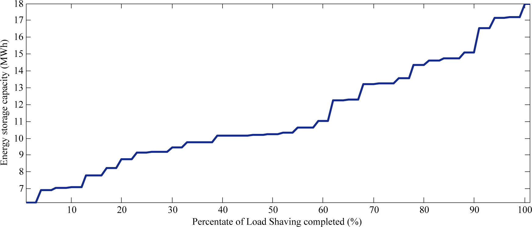
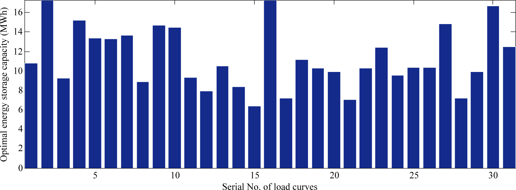
Figure 3 shows the optimal energy capacity to accomplish the tasks of peak load shaving with the power capacity being 4 MW. From the results shown in the figure, we find the energy capacity needed mainly lie in the interval from 8 to 16 MWh, that is, the system keeps discharging for 2–4 h at the maximum discharging power.

Figure 4 presents the relationships between the capacity E_cap and the peak load shaving completion rates p. The p value indicates the percentage of days with successful shaving tasks with regard to the total observed days as shown in follows:

$$p=\frac{\text{number}\text{of}\text{days}\text{with}\text{completed}\text{load}\text{shaving}\text{tasks}}{\text{number}\text{of}\text{total}\text{days}\text{studied}}$$

(23)

For example, if E_cap is 12 MWh, then the numerator would be the number of days whose optimal energy storage capacity is under 12 MWh in Figure 3. The bigger p is, the larger capacity is required. This parameter is a requirement for realistic operation considerations. A small p will increase the probability of failing to complete the peak load shaving tasks, making it necessary to expand the power system, which incurs a large amount of cost despite that the operation cost for BESS decreases. The selection of p is based on the trade-off between the two costs, which is beyond the scope of this study.

5.3. Load Forecasting Results

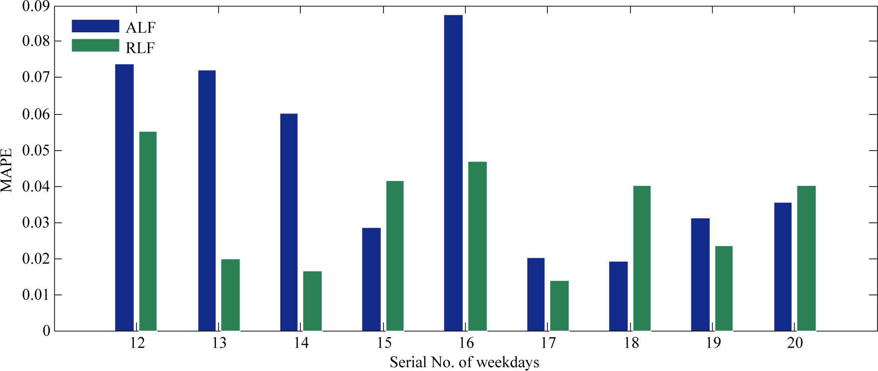
Historical data with m days backward and the known data of the day to predict are necessary for the RLF. In the simulation process, we obtain the load data of the virtual day before the next prediction point, together with the data of the preceding m virtual days, to predict the load of subsequent virtual days. We distinguish weekdays and weekend days regarding their differences in load characteristics by assigning 10 to m for weekdays and 4 for weekend days, so that we have data of the preceding two weeks in both situations. Figure 5 shows the prediction results of nine weekdays (from 18th to 21st and from 24th to 28th of March), with the average MAPEs of ALF and RLF being 4.76% (the average value of values of blue bars) and 3.31% (the average value of values of green bars) respectively. Compared with ALF, the RLF have better performances in terms of accuracy. Similar results are observed in the prediction results of weekend days.

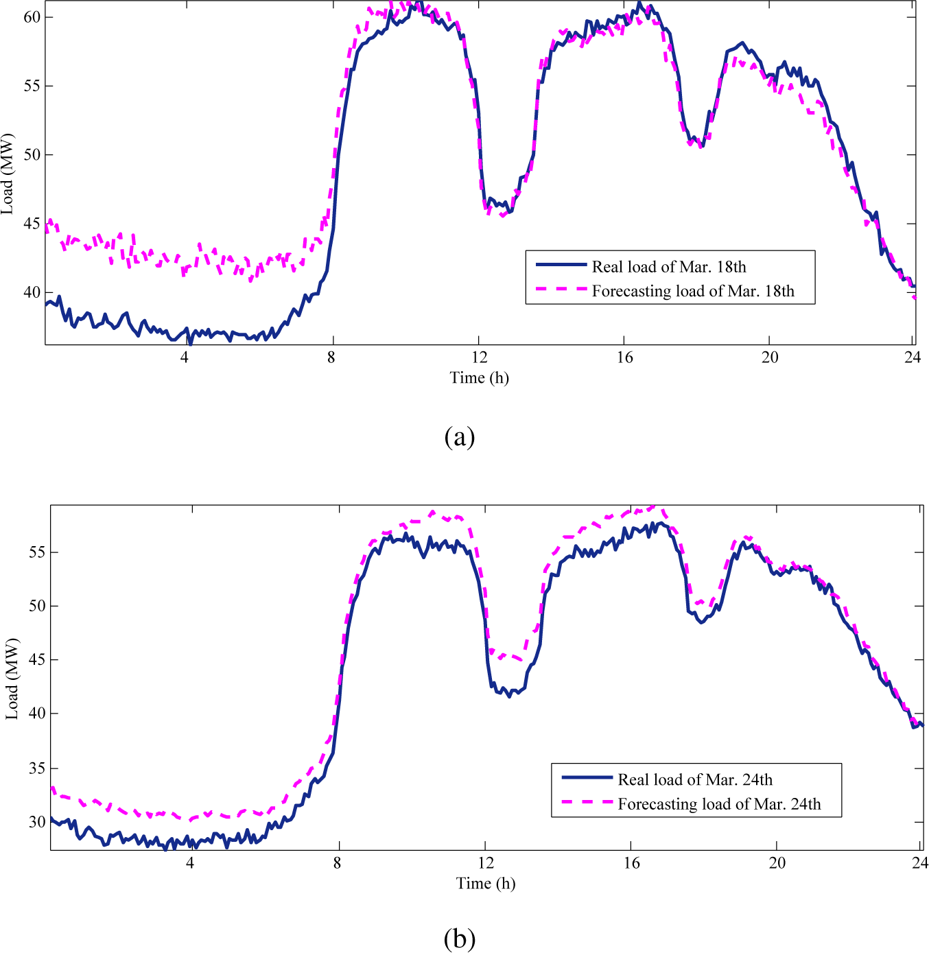
Figure 6 draws a typical curve of real and forecasting load, of the 12th weekday (March 18th) and the 16th weekday (March 24th), the latter of which has higher accuracy as we intentionally selected March 18th as a representative day with high prediction errors so as to construct a stricter criterion to validate the RLF method.

5.4. Peak Load Shaving Results

In the simulation in this section, the power capacity is set to be 4 MW and maximum charging and discharging power are assumed to be equal. The rated energy capacity is 16 MWh, and the initial remaining energy is 10% of the energy capacity All other parameters remain the same as Section 5.2.

5.4.1. Optimization Results of Different Models

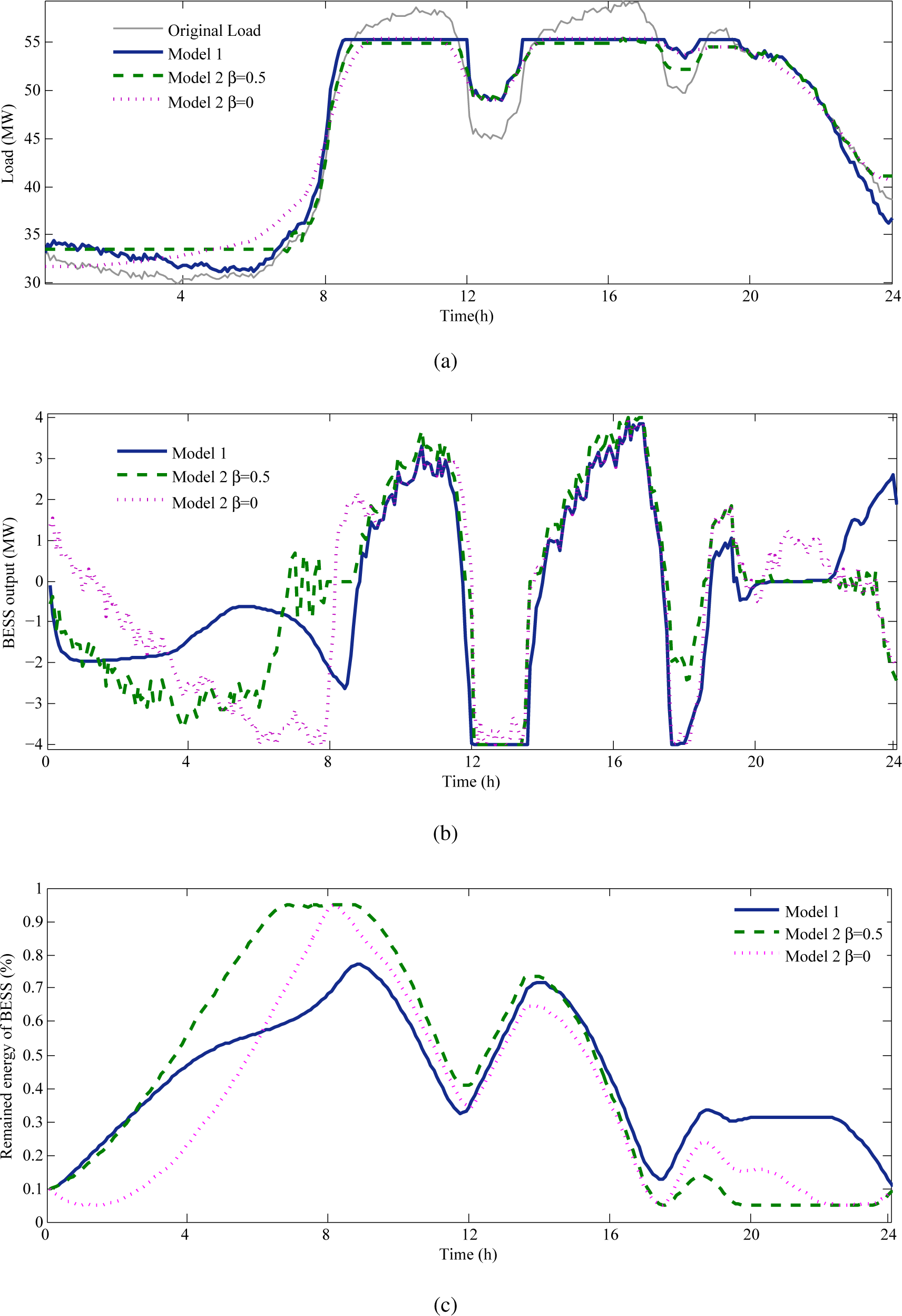
In the first simulation model, α is equal to 1, and P_level1 is 4 MW. In model 2, γ₁ of constraint (21) is equal to 1 with γ₂ equal to 0. We do not restrict the number of charging and discharging cycles in this section. Figure 7 shows the results.

Figure 7a presents the load before and after the peak load shaving. As for the load compensation in valley hours, the figure shows that, with β equal to 0.5 in model 2, the variance of the whole day’s load is considered in the objective, thus the load is compensated to a relatively high level in the valley hours to lower the variance. If β is equal to 0, the objective is solely to reduce the adjacent-time fluctuations, where we can observe a curve much more smooth but with lower level of compensation in valley hours. Model 1 completely targets load reduction in peak hours, hence for this reason it is weak in the compensation of load in valley hours. On the other hand, during the peak hours, as the peak load reduction is constrained in model 2, it will always be the case that the reduction meets the requirement whatever β is. When β is equal to 0.5 in model 2, the average value of load in peak hours is less than the other two situations after the peak load. When β is equal to 0, however, the curve becomes smooth after peak load shaving.

Figure 7b shows the BESS output under different models. It seems that the variation is lower than in model 1, since there is no need to alter output frequently to suppress the fluctuation. The only goal in model 1 is to reduce peak load to a certain level, in contrast to models aiming at to decrease the variance or reduce the adjacent-time fluctuation.

Figure 7c shows the remaining energy under different models. The number of charging and discharging cycles is the least in model 1 since it is only required to accomplish tasks of peak load shaving. On the other hand, model 2 needs more cycles and larger depth of discharge in order to reduce the variance and fluctuation.

Model 1 is recommended if only peak load shaving is required. When fluctuation reduction is also required, the model 2 with β equal to 0.5 may be more appropriate.

5.4.2. Actual Effectiveness of Peak Load Shaving

The optimization on charging and discharging power is based on the predicted load curve. However, the forecasted value always differs from the real value, which incurs a gap between the predicted effectiveness and the realized effectiveness of peak load shaving. To simulate the realized effectiveness of peak load shaving, model 2 with β equal to 0.5, γ₁ equal to 1 and γ₂ equal to 0 are adopted to do the analysis. The constraint of charging and discharging cycles is removed.

Table 1. Valley compensation of weekdays and weekend days.

Peak Load Reduction = 4 MW
Weekdays	Pv_com	Pmax_vload	Rv_com	Cycles	Weekend days	Pv_com	Pmax_vload	Rv_com	Cycles
18 March	2.67	11.04	0.24	1.44	16 March	2.26	7.63	0.30	1.27
19 March	2.61	13.63	0.19	1.37	22 March	2.48	9.03	0.27	1.32
20 March	2.67	13.03	0.20	1.38	23 March	2.20	7.77	0.28	1.30
21 March	3.41	14.54	0.23	1.39	29 March	2.59	9.38	0.27	1.34
24 March	3.33	15.95	0.21	1.34	30 March	2.52	9.46	0.27	1.37
25 March	1.76	12.74	0.14	1.41
26 March	3.38	14.68	0.23	1.34
27 March	3.18	12.56	0.25	1.35
28 March	3.21	12.12	0.27	1.35
31 March	2.93	13.18	0.22	1.35
Average	2.92	13.35	0.22	1.37	Average	2.41	8.65	0.28	1.32

Notes: P_{v_com} is the power compensation amount in valley hours; P_{max_vload} is the maximum value of the difference between mean load and valley load; $R_{v\_com}=\frac{P_{v\_com}}{P_{max\_vload}}$ is the compensation rate.

shows the one-shot optimization results of 10 weekdays and 5 weekend days, using historical data of the first 11 weekdays (from 3 March to 7 March, 10 March to 14 March and 17 March) and 5 weekend days (i.e., 1 March, 2 March, 8 March, 9 March and 15 March). In these applications, the energy capacity is fixed and we require that the peak load reduction be 4 MWh, such that we focus on the valley compensation and charging and discharging cycles. We use the percentage of valley compensation on the difference between the mean load and the lowest load as an index. On average, 22% of the valley load is compensated on weekdays and 28% of the valley load is compensated for weekend days, and the cycles are slightly more than 1.3. The results of weekend days are better than weekdays because the load variation is smaller in weekend days under the same energy capacity. It is noted that all the optimizations are achieved with a fixed energy capacity, and the results may still get better if we increase the energy capacity.

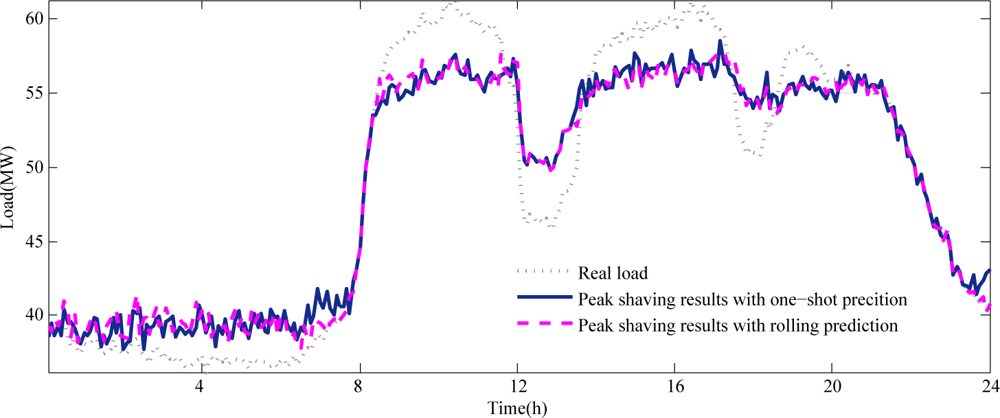
However, the optimization of the RLF method is even better than the one-shot method. Figure 8 displays the real effectiveness of peak load shaving of both the one-shot method and the RLF method on March 18th. With the data on 18 March 2014, the peak load reduction under one-shot optimization is 2.7496 MW but 4 MW under RLF.

Although there is difference between the predicted load curve and real load curve, the peak load shaving is still effective because the peak hours of both the curves match. As for the one-shot forecasting, the shapes of the predicted curve and that of the real curve differ a lot, especially in the valleys. Compared with one-shot optimization, the RLF method significantly increases the peak load reduction by improving the forecasting accuracy and adjusting the charging and discharging process in real-time.

6. Conclusions

In this study, an optimization model satisfying peak load reduction requirements is proposed to minimize the BESS capacity required for peak load shaving. A rolling load forecasting method is also employed to enhance the optimization performance. In addition, two charging and discharging control models are established with different optimization objectives, that is, to minimize peak–valley differences and to minimize daily load variance. By considering the penalty cost of load fluctuation in the objective function, the curve of the daily load can be smoothed simultaneously. The constraint of charging and discharging cycles is also taken into consideration, which overcomes the drawback that resulted from using the changes of charging and discharging status to represent the usage of battery. Simulations based on the real load data was carried out to validate the proposed optimization models and control strategies. The results show that improved peak load shaving performances can be achieved with limited BESS capacity.

References

- Divya, K.; Østergaard, J. Battery energy storage technology for power systems-an overview. Electr. Power Syst. Res 2009, 79, 511–520. [Google Scholar]
- Vazquez, S.; Lukic, S.M.; Galvan, E.; Franquelo, L.G.; Carrasco, J.M. Energy storage systems for transport and grid applications. IEEE Trans. Ind. Electron 2010, 57, 3881–3895. [Google Scholar]
- Hida, Y.; Yokoyama, R.; Shimizukawa, J.; Iba, K.; Tanaka, K.; Seki, T. Load Following Operation of Nas Battery by Setting Statistic Margins to Avoid Risks, Proceedings of the 2010 IEEE Power and Energy Society General Meeting, Minneapolis, MN, USA, 25–29 July 2010; pp. 1–5.
- Niu, D.; Shi, H.; Li, J.; Wei, Y. Research on Short-Term Power Load Time Series Forecasting Model Based on bp Neural Network, Proceedings of the 2010 2nd International Conference on Advanced Computer Control (ICACC), Shenyang, Liaoning, China, 27–29 March 2010; pp. 509–512.
- Liu, K.; Subbarayan, S.; Shoults, R.; Manry, M.; Kwan, C.; Lewis, F.; Naccarino, J. Comparison of very short-term load forecasting techniques. IEEE Trans. Power Syst 1996, 11, 877–882. [Google Scholar]
- Lee, T.-Y. Operating schedule of battery energy storage system in a time-of-use rate industrial user with wind turbine generators: A multipass iteration particle swarm optimization approach. IEEE Trans. Energy Conver 2007, 22, 774–782. [Google Scholar]
- Chacra, F.A.; Bastard, P.; Fleury, G.; Clavreul, R. Impact of energy storage costs on economical performance in a distribution substation. IEEE Trans. Power Syst 2005, 20, 684–691. [Google Scholar]
- Fung, C.; Ho, S.; Nayar, C. Optimisation of a Hybrid Energy System Using Simulated Annealing Technique, Proceedings of the 1993 IEEE Region 10 Conference on Computer, Communication, Control and Power Engineering (TENCON’93), 9–21 October 1993; pp. 235–238.
- Oudalov, A.; Cherkaoui, R.; Beguin, A. Sizing and Optimal Operation of Battery Energy Storage System for Peak Shaving Application, Proceedings of the 2007 IEEE Lausanne Power Tech, Lausanne, Switzerland, 1–5 July 2007; pp. 621–625.
- Maly, D.; Kwan, K. Optimal battery energy storage system (BESS) charge scheduling with dynamic programming. IEEE Proc. Sci. Meas. Technol 1995, 142, 453–458. [Google Scholar]
- Chen, S.; Gooi, H.B.; Wang, M. Sizing of energy storage for microgrids. IEEE Trans. Smart Grid 2012, 3, 142–151. [Google Scholar]
- Guan, X.; Xu, Z.; Jia, Q.-S. Energy-efficient buildings facilitated by microgrid. IEEE Trans. Smart Grid 2010, 1, 243–252. [Google Scholar]
- Ding, M.; Xu, N.; Lin, G. Static function of the battery energy storage system. Trans. China Electrotech. Soc 2012, 27, 242–248. [Google Scholar]
- Xie, L.; Thatte, A.; Gu, Y. Multi-time-scale modeling and analysis of energy storage in power system operations, Proceedings of the 2011 IEEE Energytech, Cleveland, OH, USA, 25–26 May 2011; pp. 1–6.
- Kerestes, R.J.; Reed, G.F.; Sparacino, A.R. Economic analysis of grid level energy storage for the application of load leveling, Proceedings of the 2012 IEEE Power and Energy Society General Meeting, San Diego, CA, USA, 22–26 July 2012; pp. 1–9.
- Papic, I. Simulation model for discharging a lead-acid battery energy storage system for load leveling. IEEE Trans. Energy Conver 2006, 21, 608–615. [Google Scholar]
- Lo, C.H.; Anderson, M.D. Economic dispatch and optimal sizing of battery energy storage systems in utility load-leveling operations. IEEE Trans. Energy Conver 1999, 14, 824–829. [Google Scholar]