Ground Return Current Behaviour in High Voltage Alternating Current Insulated Cables

 ,
,  ,
,
Abstract
:1. Introduction
- ➢
- EHV overhead lines with any number of earth wires [1];
- ➢
- Milliken conductors [2];
- ➢
- Harmonic behaviour of high voltage direct current (HVDC) cables [3];
- ➢
- Distribution line carrier (DLC) in medium voltage (MV) network [4];
- ➢
- Alternating current (AC) gas Insulated transmission Lines (GILs) [5];
- ➢
- AC high-speed railway supply [6].
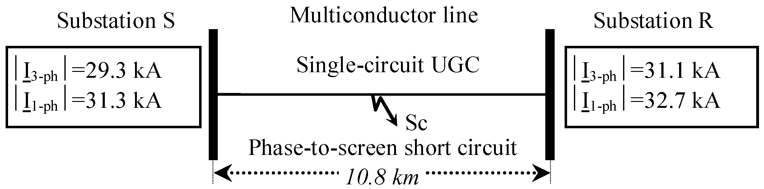
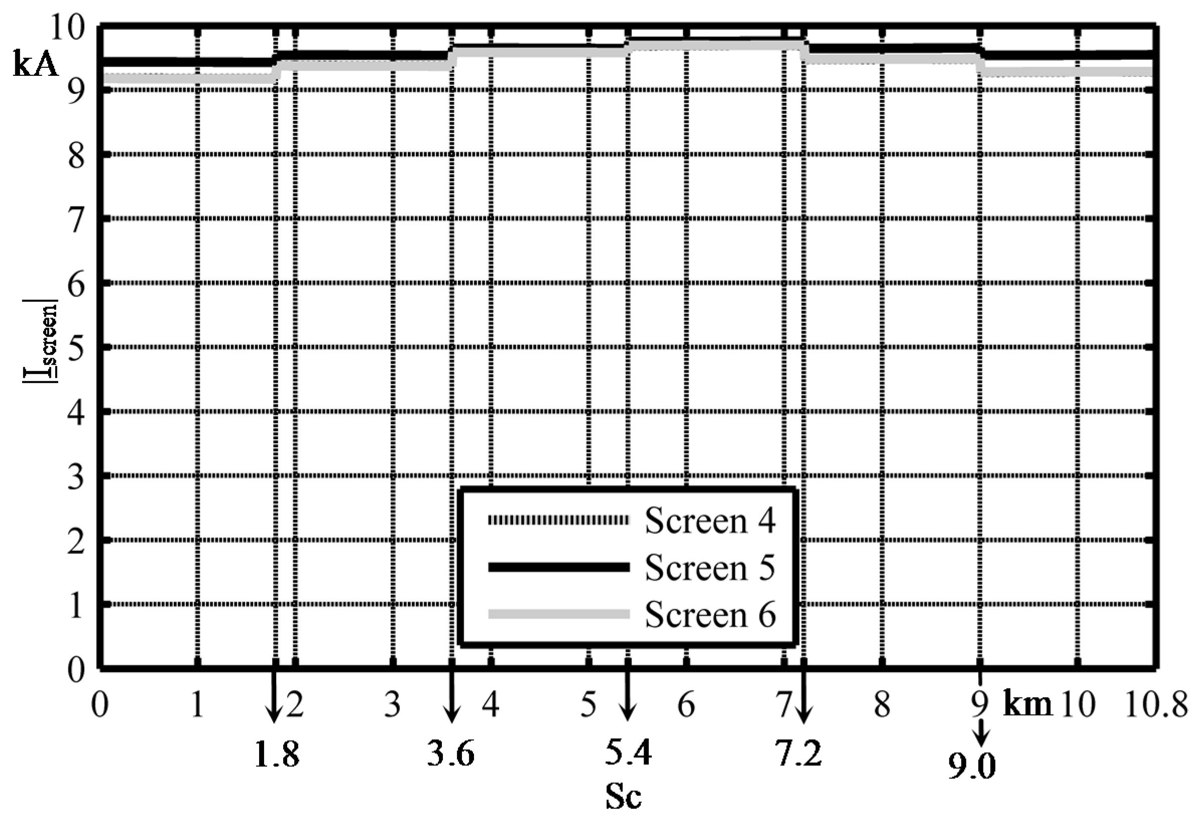
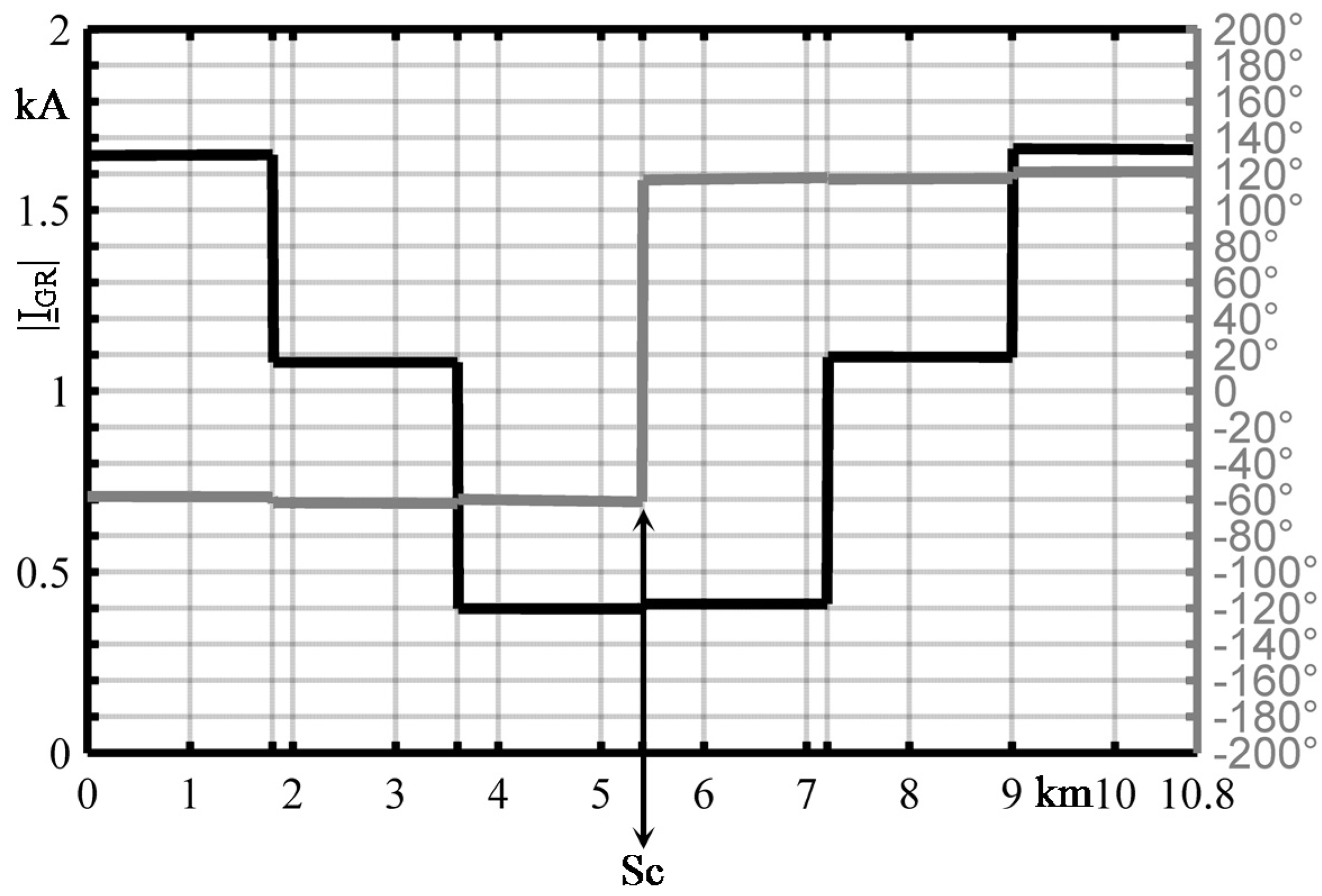
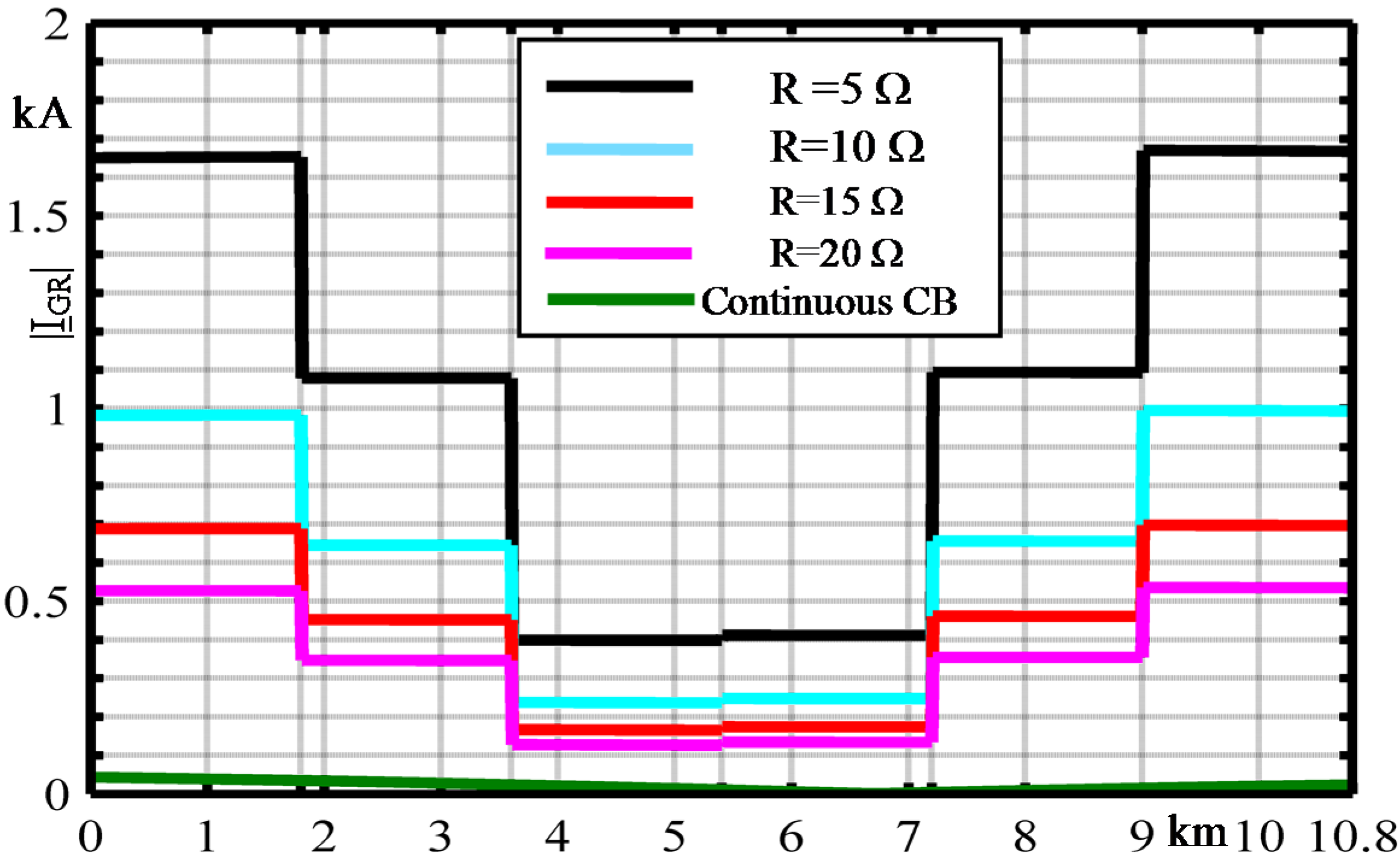
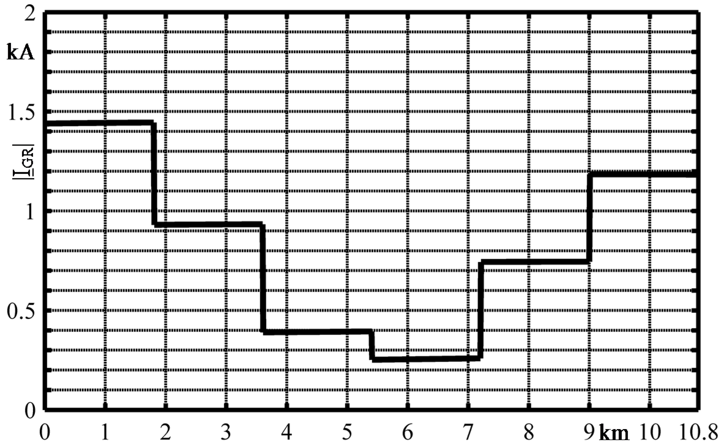
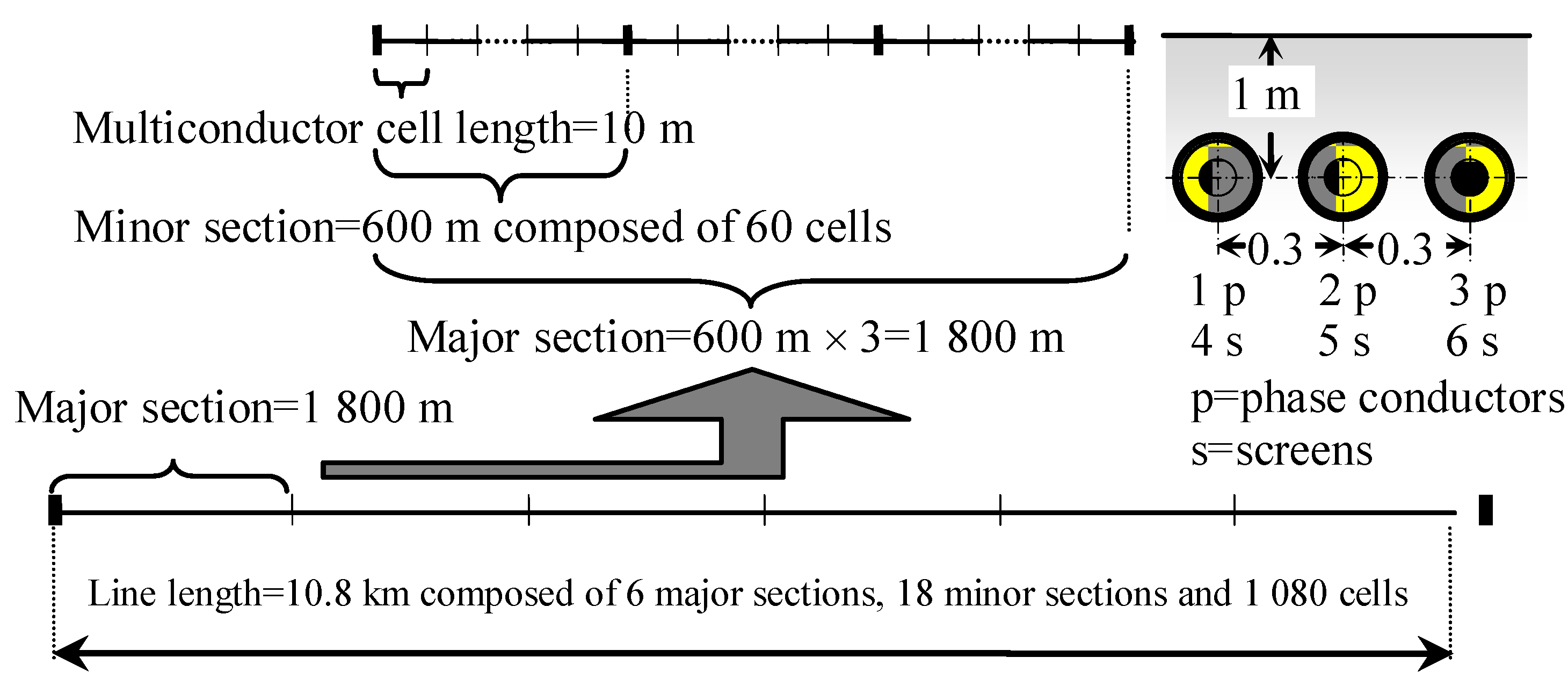
2. Fault Occurrence in a Cross-Bonded Single Circuit Cable Line by Means of Multiconductor Cell Analysis


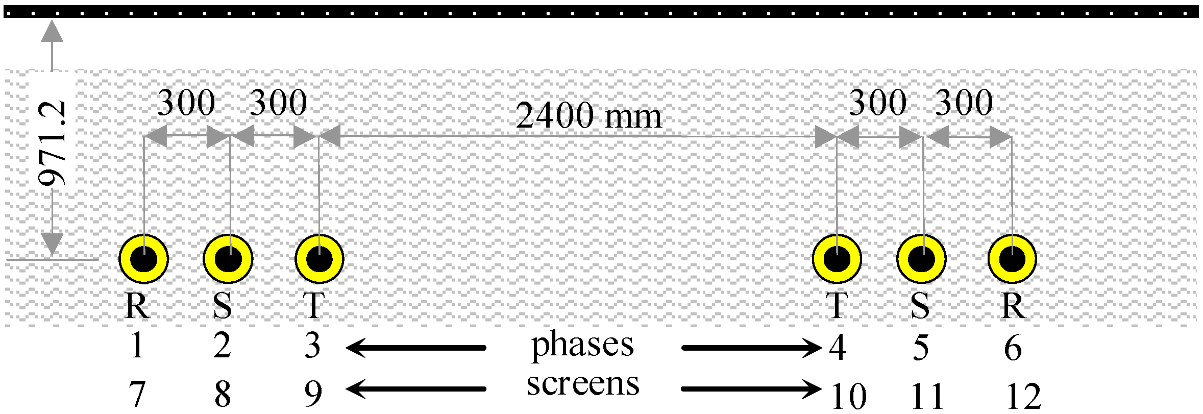
| Cable type insulation | Unit | XLPE |
|---|---|---|
| Voltage levels after IEC 62067 | kV | 220/380 (420) |
| Cross sectional area/material | mm2 | 2500/Cu M-type |
| Conductor diameter | mm | 64.3 |
| Conductor screen diameter d0 | mm | 68.7 |
| Insulation diameter d1 | mm | 122.8 |
| Insulation screen diameter | mm | 126.1 |
| Metallic shield diameter/material | mm | 131.3/Al welded |
| Jacket of PE diameter | mm | 142.4 |
| Overall diameter | mm | 142.4 |
| Per unit length 50 Hz resistance of phase conductor at 20 °C | mΩ/km | 8.4827 |
| Per unit length series Inductance | mH/km | 0.5431 |
| Per unit length shunt Leakance (50 Hz) with loss factor tanδ = 0.0007 | nS/km | 48.4 |
| Per unit length shunt Capacitance with εr = 2.3 | μF/km | 0.22 |
| Per unit length zero sequence impedance z0 | Ω/km | 0.0547 + j·0.0612 |
| Line length | km | 10.8 |
| Cell length | m | 10 |
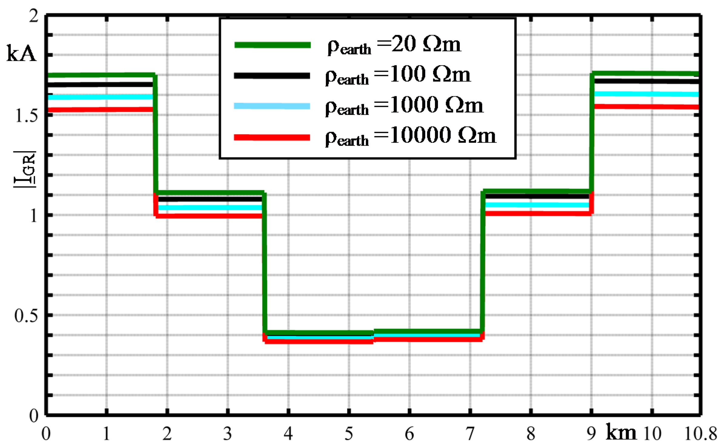
| Earth resistivity | Ω·m | 100 |
| Substation earthing resistances RA and RB | Ω | 0.1 |
| Major section CB box resistance R | Ω | 5 |
| Link resistance Rcont between screens at earthing sites | mΩ | 1 |


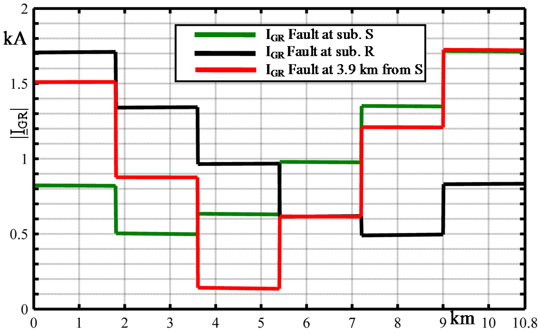
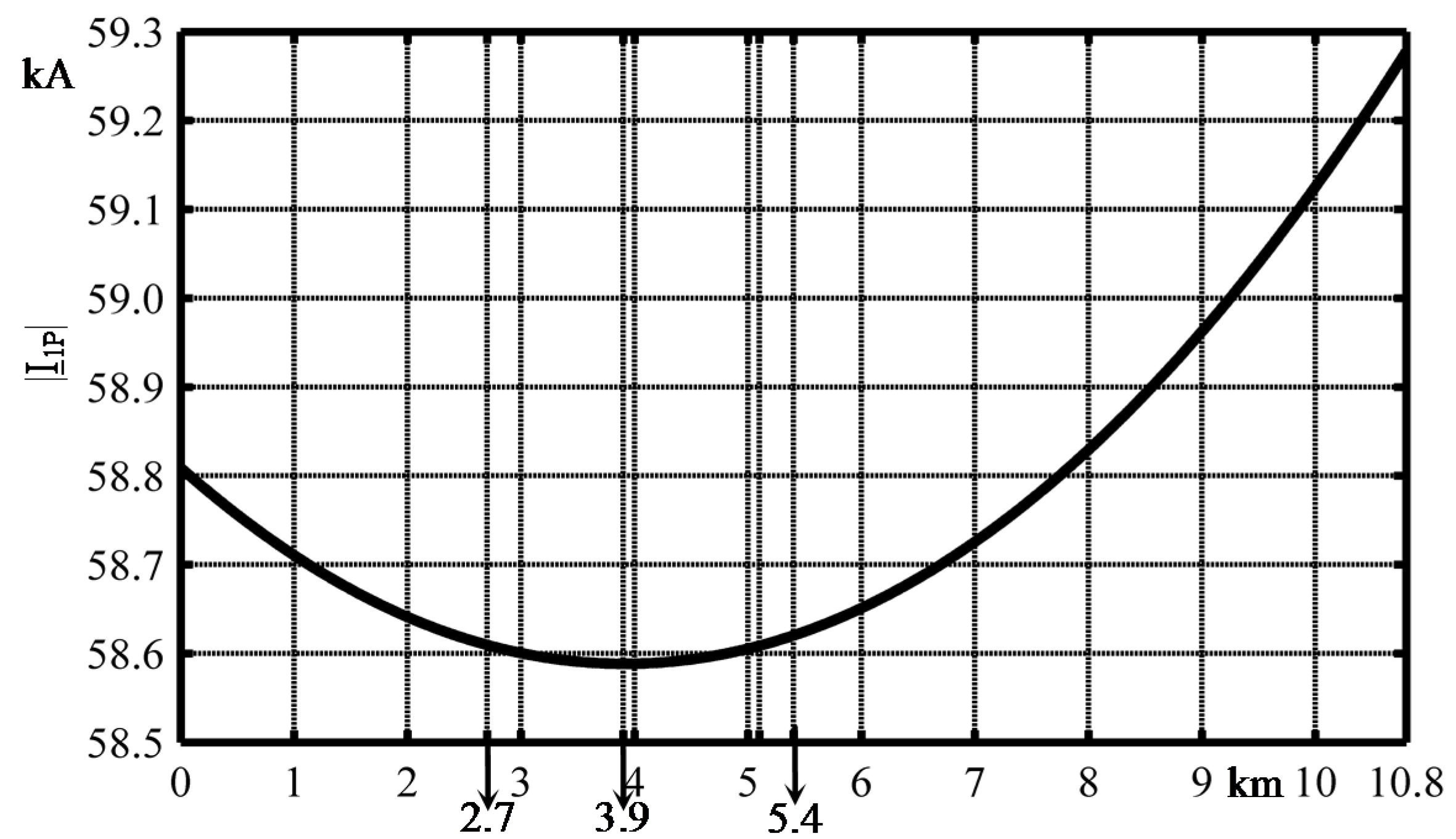
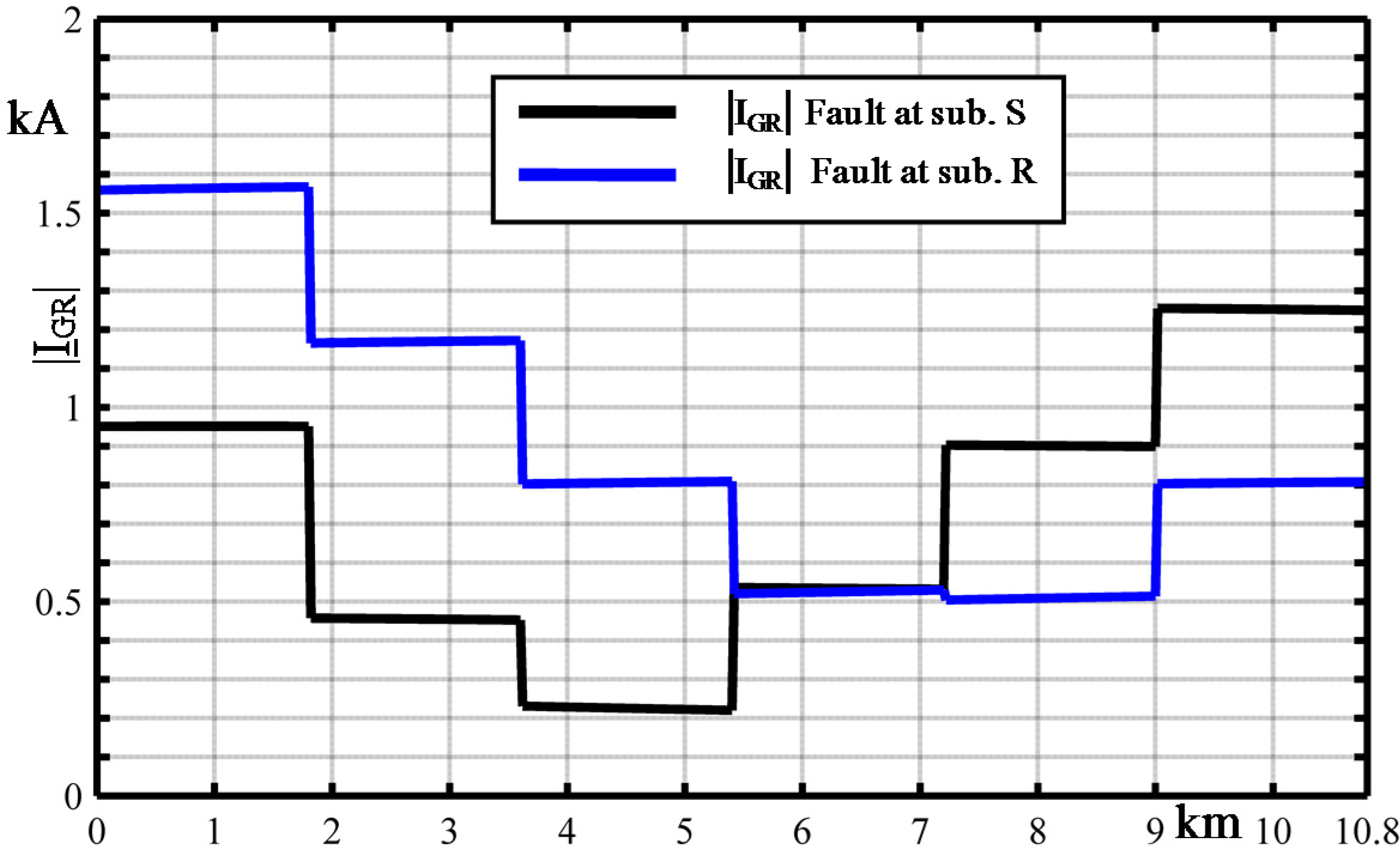
- at S substation;
- at R substation;
- at 3.9 km from S substation.
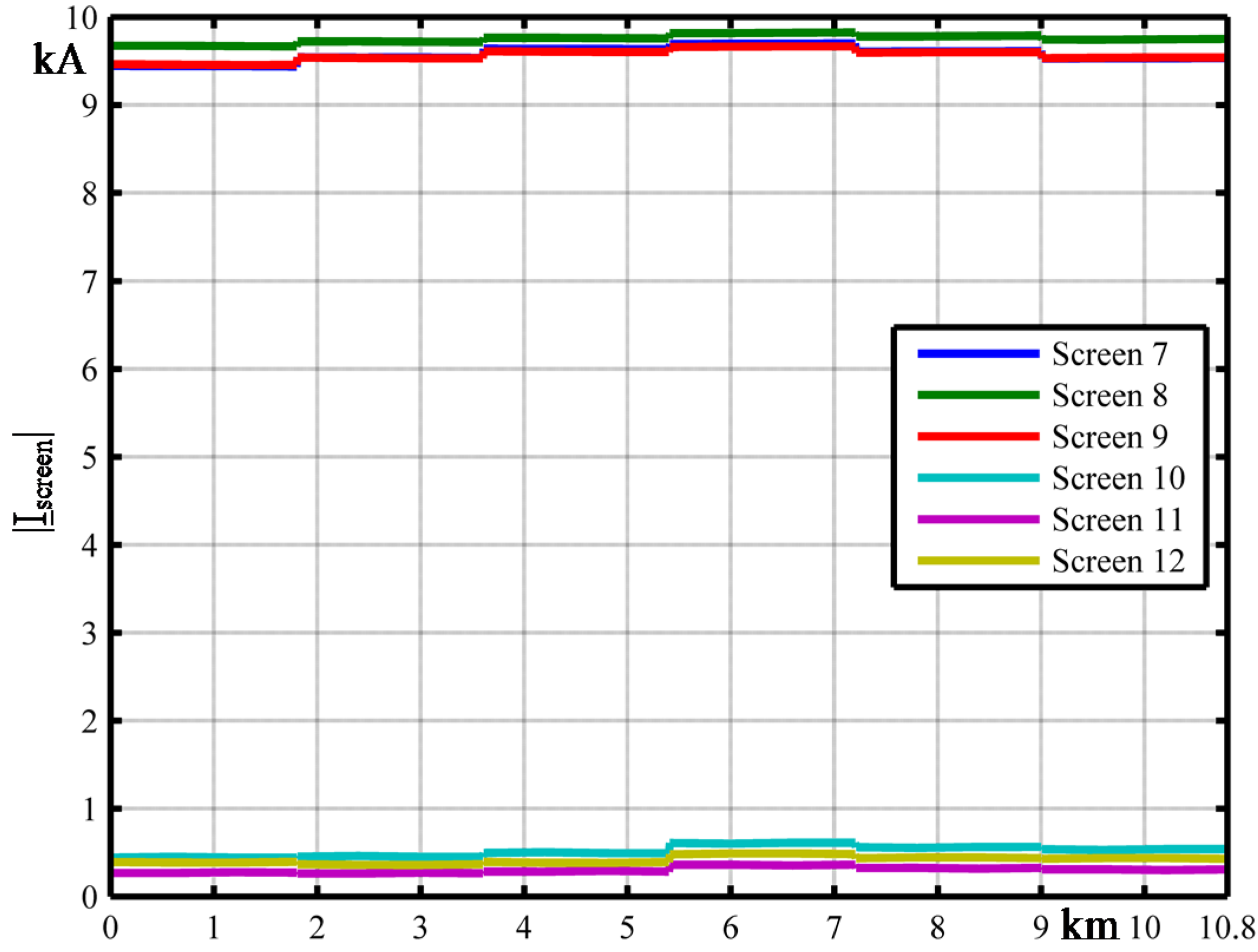
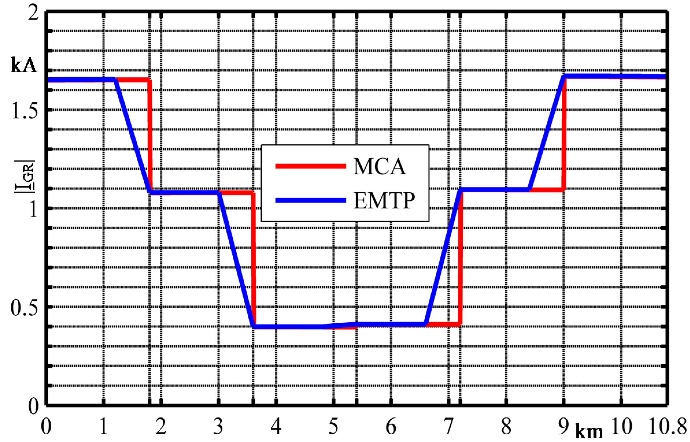
Ground Return Current in Double Circuit Underground Cable


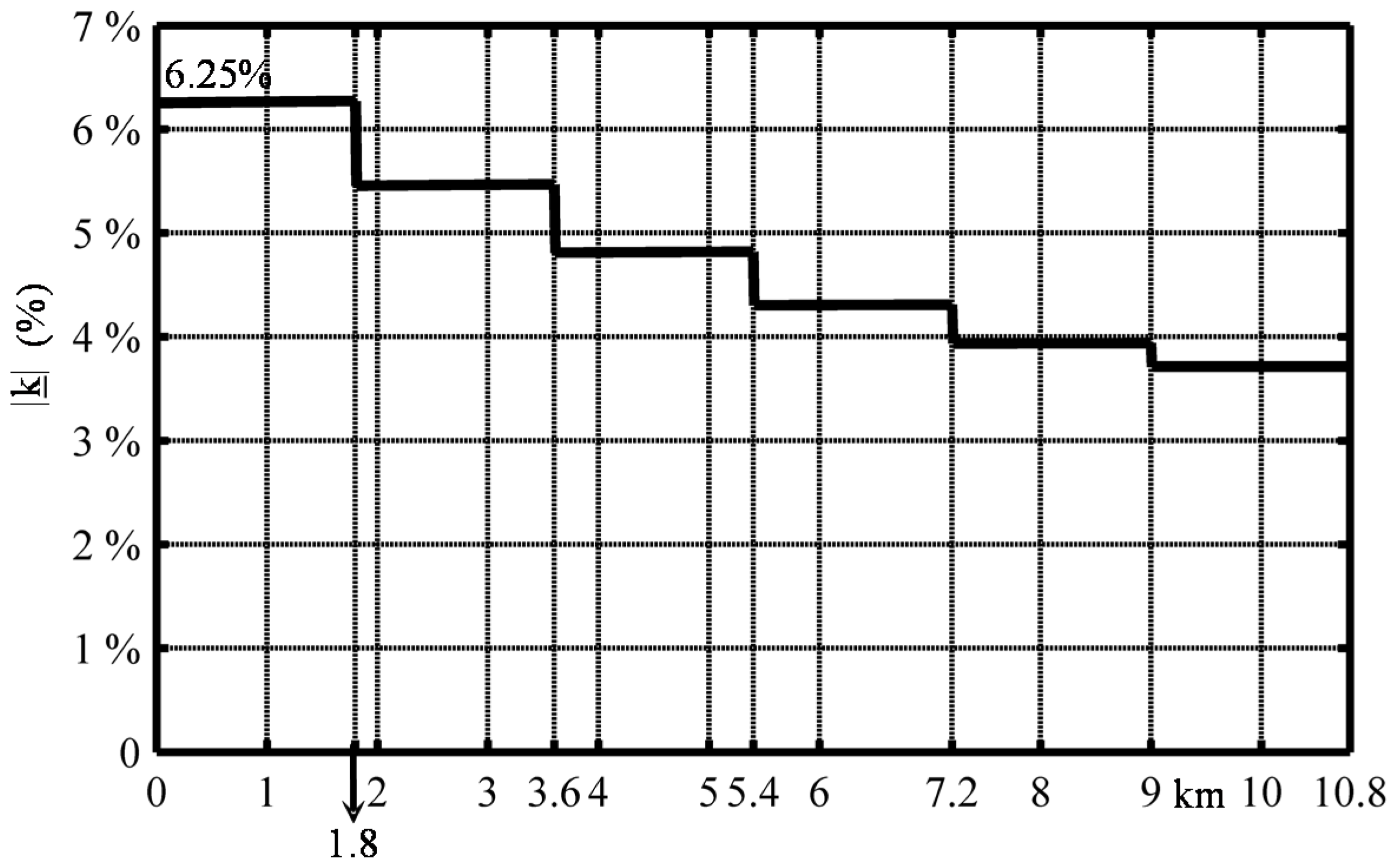
3. Comparison with k-Factors

| Short circuit location | |k| L.M. Popović | |k| MCA |
|---|---|---|
| 0.0083 | 0.0082 | |
| 0.0166 | 0.0165 | |
| 0.0249 | 0.0248 |
3.1. Cross-Bonded Cable
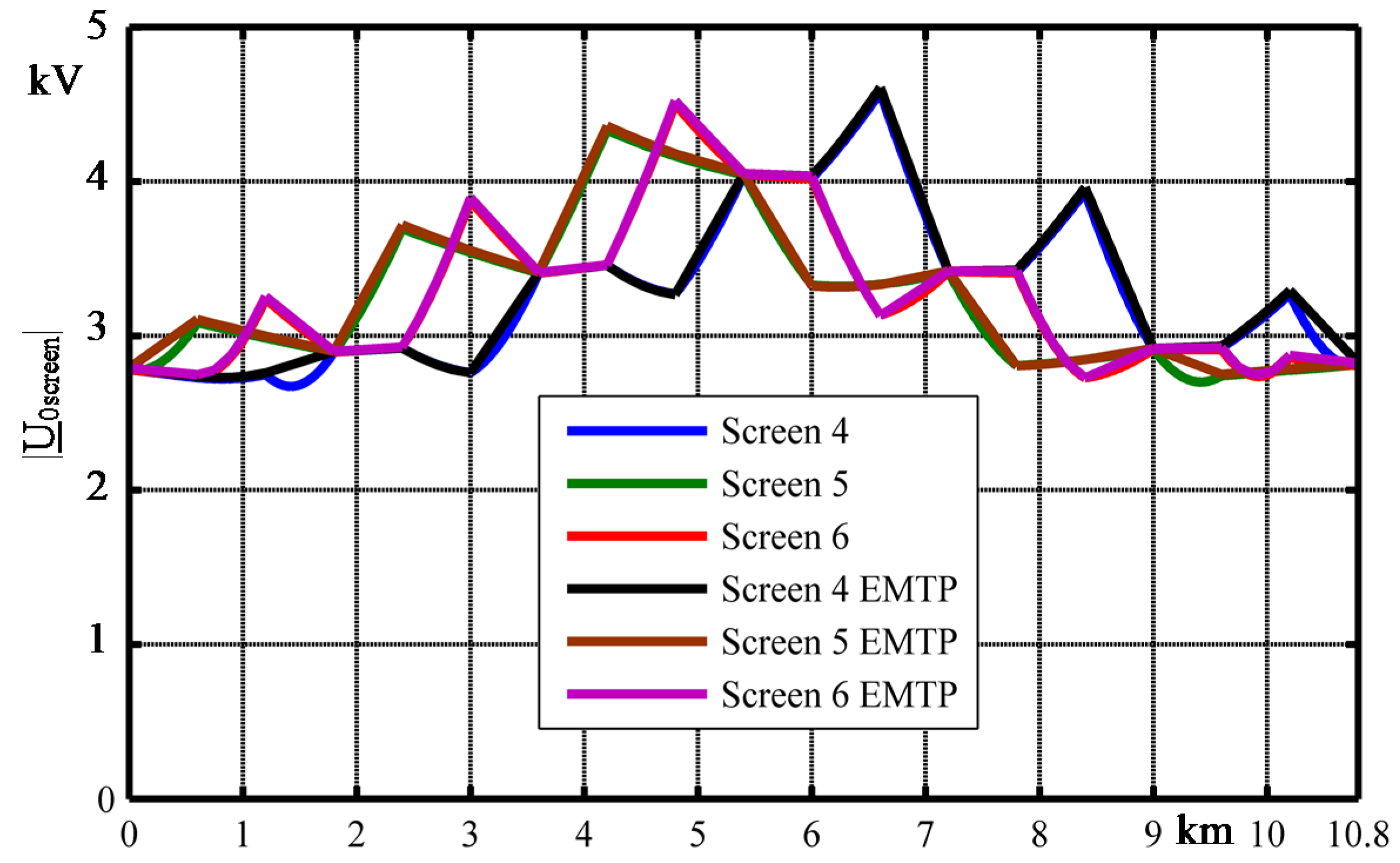
4. Comparison with ElectroMagnetic Transient Program-Restructured Version

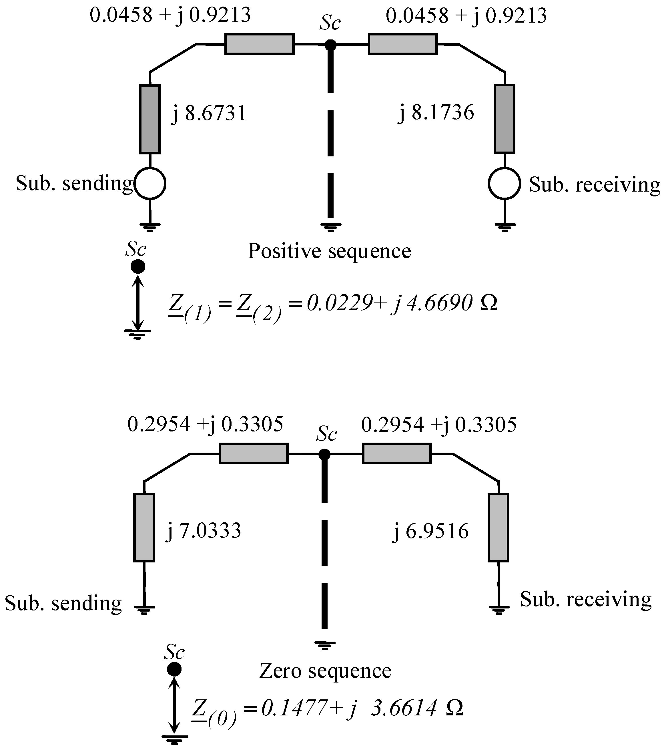
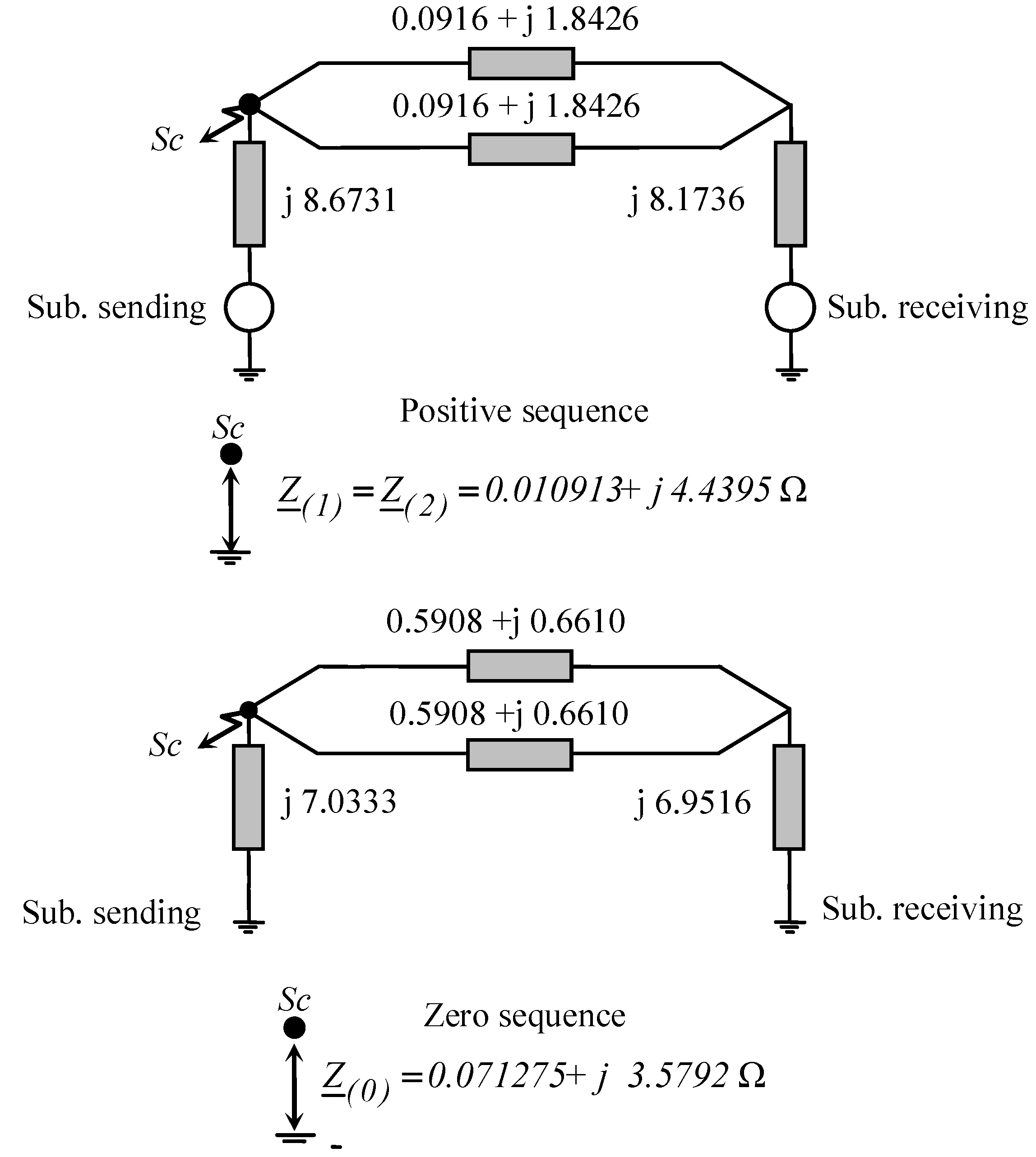
5. Comparison with Sequence Theory


| CB fault location Faulted screen 8 with corresponding phase 2 | MCA (kA) | SI (kA) | |
|---|---|---|---|
| Substation S | 61.186 | 61.171 | 0.0245 |
| Substation R | 61.438 | 61.436 | 0.0033 |
| 5.4 km from Sub. S | 58.619 | 58.622 | −0.0051 |
6. Conclusions
- ➢
- ➢
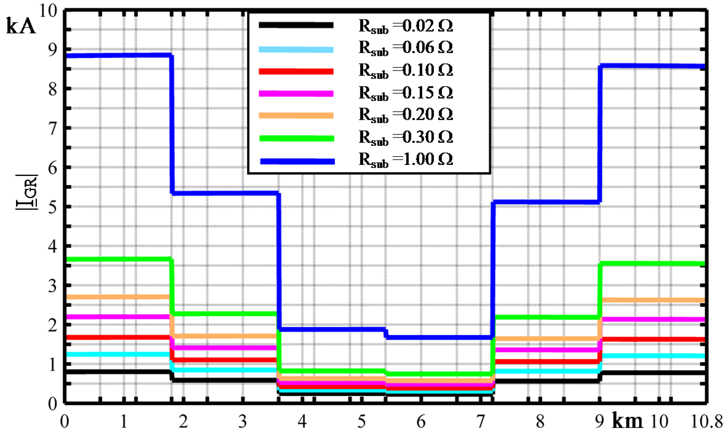
- The short circuit |IGR| is significantly influenced by the different values of both the major section CB box resistances and the substation grid ones since the metallic screens are earthed at each major section and at the substation sites: the lower the value of substation grid resistances the lower the magnitude of ground return current;
- ➢
- The use of sequence impedance approach only for short circuit computations gives slight errors since the transposed UGCs are a rather symmetric system. Of course, the sequence theory approach cannot give |IGR|;
- ➢
- The double-circuit UGC gives (in the same conditions of single-circuit UGC) lower ground return current magnitudes;
- ➢
- k-factors are valid for solid bonded cables. They are not applicable to cross-bonded UGCs whether single-circuit or a double- circuit;
- ➢
- IEC 60909-2 and 60909-3 give k-factors only for solid bonded three single-core cables laid in trefoil and flat configurations so that no evaluation is possible for cross-bonded cables which are the usual screen arrangement of HV-EHV cables. IEC k-factor applied to SB cables in flat laying gives an underestimate of about 10%.
Conflicts of Interest
References
- Benato, R.; Sessa, S.D.; Guglielmi, F. Determination of steady-state and faulty regimes of overhead lines by means of multiconductor cell analysis (MCA). Energies 2012, 5, 2771–2793. [Google Scholar] [CrossRef]
- Benato, R.; Paolucci, A. Multiconductor cell analysis of skin effect in Milliken type cables. Electr. Power Syst. Res. 2012, 90, 99–106. [Google Scholar] [CrossRef]
- Benato, R.; Forzan, M.; Marelli, M.; Orini, A.; Zaccone, E. Harmonic behaviour of HVDC cables. Electr. Power Syst. Res. 2012, 89, 215–222. [Google Scholar] [CrossRef]
- Benato, R.; Caldon, R. Distribution line carrier: Analysis procedure and applications to distributed generation. IEEE Trans. Power Deliv. 2007, 22, 575–583. [Google Scholar] [CrossRef]
- Benato, R.; di Mario, C.; Koch, H. High capability applications of long gas insulated lines in structures. IEEE Trans. Power Deliv. 2007, 22, 619–626. [Google Scholar] [CrossRef]
- Benato, R.; Caldon, R.; Paolucci, A. Matrix algorithm for the analysis of high speed railway and its supply system. L’Energ. Elettr. 1998, 75, 304–311. (In Italian) [Google Scholar]
- Benato, R. Multiconductor analysis of underground power transmission systems: EHV AC cables. Electr. Power Syst. Res. 2009, 79, 27–38. [Google Scholar] [CrossRef]
- Popović, L.M. Determination of the reduction factor for feeding cables consisting of three single-core cables. IEEE Trans. Power Deliv. 2003, 18, 736–743. [Google Scholar] [CrossRef]
- Sarajcev, I.; Majstrovic, M.; Sutlovic, E. Influence of earthing conductors on current reduction factor of a distribution cable laid in high resistivity soil. In Proceedings of the 2001 IEEE Power Tech Conference, Porto, Portugal, 10–13 September 2001.
- Sarajcev, I.; Majstrovic, M.; Sutlovic, E. Determining currents of cable sheaths by means of current load factor and current reduction factor. In Proceedings of the 2003 IEEE Power Tech Conference, Bologna, Italy, 23–26 January 2003.
- Sarajcev, I.; Majstrovic, M.; Medic, I. Current reduction factor of compensation conductors laid alongside three single-core cables in flat formation. In Proceedings of the 2003 IEEE International Symposium on Electromagnetic Compatibility, Istanbul, Turkey, 11–16 May 2003.
- Popović, L.M. Practical method for evaluating ground fault current distribution in station, towers and ground wire. IEEE Trans. Pow. Deliv. 1998, 13, 123–128. [Google Scholar] [CrossRef]
- Popović, L.M. Efficient reduction of fault current through the grounding grid of substation supplied by cable line. IEEE Trans. Pow. Deliv. 2000, 15, 556–561. [Google Scholar] [CrossRef]
- Popović, L.M. Ground fault current distribution in stations supplied by a line composed of a cable and an overhead section. Eur. Trans. Electr. Power 2007, 17, 207–218. [Google Scholar] [CrossRef]
- Popović, L.M. Determination of actual reduction factor of HV and MV cable lines passing through urban and suburban areas. Electron. Energ. 2014, 27, 25–39. [Google Scholar]
- Popović, L.M. Ground fault current distribution for the fault anywhere along the feeding line consisting of three single-core cables. In Proceedings of the Sixth International Symposium Nikola Tesla, Belgrade, Serbia, 18–20 October 2006.
- Popović, L.M. Improved analytical expressions for the reduction factor of feeding lines consisting of three single-core cables. Eur. Trans. Electr. Power 2008, 18, 190–203. [Google Scholar] [CrossRef]
- Viel, E.; Griffiths, H. Fault current distribution in HV cable systems. IEEE Proc. Gener. Transm. Distrib. 2000, 147, 231–238. [Google Scholar] [CrossRef]
- Viel, E.; Griffiths, H. Determination of ground return currents for earth faults fed by metal sheathed/screened cables. A Case Study. In Proceedings of the 33rd Universities Power Engineering conference, UPEC’ 98, Edinburgh, UK, 8–10 September 1998; pp. 715–718.
- Short-Circuit Currents in Three-Phase a.c. Systems—Part 2: Data of Electrical Equipment for Short-Circuit Current CalculationsIEC/TR 60909-2, Ed. 2.0 ed; International Electrotechnical Commission (IEC): Geneva, Switzerland, 2008.
- Short-Circuit Currents in Three-Phase a.c. Systems—Part 3: Currents during Two Separate Simultaneous Line-to-Earth Short-Circuits and Partial Short-Circuit Currents Flowing through EarthIEC 60909-3, Ed. 2.0 ed; International Electrotechnical Commission (IEC): Geneva, Switzerland, 2003.
- Short-Circuit Currents in Three-Phase a.c. Systems—Part 0: Calculation of CurrentsIEC 60909-0, Ed. 1.0 ed; International Electrotechnical Commission (IEC): Geneva, Switzerland, 2001.
- Sutton, S.; Plath, R.; Schröder, G. The St. Johns wood—elstree experience—testing a 20 km long 400 kV XLPE-insulated cable system after installation. In Proceedings of the 7th International Conference on Insulated Power Cable JiCable07, Versailles, France, 24–28 June 2007.
- Sadler, S.; Sutton, S.; Memmer, H.; kaumanns, J. 1600 MVA electrical power transmission with an EHV XLPE cable system in the underground of London. In Proceedings of the Cigrè 2004, Paris, France, 29 August 2004.
- Tsuchiya, S.; Iida, T.; Morishita, Y.; Tnkajim, A.; Akiya, Y.; Kurata, T. EHV cable installation technology for tunnels and ducts in Japan. In Proceedings of the Cigré 2012, Paris, France, 26 August 2012.
- Benato, R.; Caciolli, L. Sequence impedances of insulated cables: Measurements versus computations. In Proceedings of the Transmission and Distribution Conference and Exposition (T&D), 2012 IEEE PES, Orlando, FL, USA, 7–10 May 2012.
© 2014 by the authors; licensee MDPI, Basel, Switzerland. This article is an open access article distributed under the terms and conditions of the Creative Commons Attribution license (http://creativecommons.org/licenses/by/4.0/).
Share and Cite
Benato, R.; Sessa, S.D.; Guglielmi, F.; Partal, E.; Tleis, N. Ground Return Current Behaviour in High Voltage Alternating Current Insulated Cables. Energies 2014, 7, 8116-8131. https://doi.org/10.3390/en7128116
Benato R, Sessa SD, Guglielmi F, Partal E, Tleis N. Ground Return Current Behaviour in High Voltage Alternating Current Insulated Cables. Energies. 2014; 7(12):8116-8131. https://doi.org/10.3390/en7128116
Chicago/Turabian StyleBenato, Roberto, Sebastian Dambone Sessa, Fabio Guglielmi, Ertugrul Partal, and Nasser Tleis. 2014. "Ground Return Current Behaviour in High Voltage Alternating Current Insulated Cables" Energies 7, no. 12: 8116-8131. https://doi.org/10.3390/en7128116