A Recursive Solution for Power-Transmission Loss in DC-Powered Networks

Abstract
: This article presents a recursive solution to the power-transmission loss in DC-powered networks. In such a network, the load cannot be modeled as a fixed equivalent resistance value, since the switching regulator may draw more or less current based on the actual supply voltage to meet the power demand. Although the power-transmission loss itself is simply I2 RL, I, in turn, depends on the load’s supply voltage, which, in turn, depends on I, making it impossible to derive a closed-form solution by classical resistive network analysis in general. The proposed approach is to first derive a closed-form solution to I in the one-node topology using the quadratic formula. Next, we extend our solution to a locally daisy-chained (LDC) network, where the network is readily decomposable into stages, such that the solution combines the closed-form formula for the current stage with the recursive solution for the subsequent stages. We then generalize the LDC topology to trees. In practice, the solution converges quickly after a small number of iterations. It has been validated on real-life networks, such as power over controller area network (PoCAN).1. Introduction
Transmission of DC power in local-area networks (LAN) is a problem of increasing importance. For example, power over Ethernet (PoE) is gaining wide acceptance in offices using IP (Internet Protocol) telephones in conjunction with routers and other Internet appliances. Another example is controller area network (CAN), a widely-used standard in automobiles, as well as industrial control. These and many other emerging wired network standards run DC power lines alongside data wires in a bundled cable, such as RJ45 or RJ9, making it convenient for deployment, as only a single modular jack needs to be plugged in without requiring a separate AC adapter brick. Moreover, the growing popularity of photovoltaic (PV) generators is suggesting in-home DC power networks either in conjunction or in lieu of the traditional AC power lines.
The amount of DC power-transmission loss in such LANs is becoming a growing part of the total load. As more devices are powered by such relatively low-voltage networks, the transmission loss can grow rapidly in the sharp-slope region of the quadratic curve. In such a network, we assume that resistive load is dominant, while capacitive or inductive effects are negligible, as we are interested in the steady-state behavior. Thus, each transmission-line segment can be modeled as an equivalent resistor in series. However, as a power consumer, a node in such a network cannot be modeled as a constant equivalent resistor, because depending on the voltage, the node draws a different amount of current for the voltage-current product to meet the power demand. Surprisingly, precise solutions for analyzing the power-transmission loss in such networks have not been published.
1.1. Failure of Resistive Network Analysis
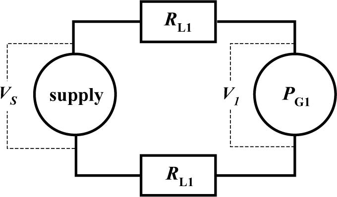
Consider a single-node network, as shown in Figure 1. The equivalent resistance RG1 of the node is a function of the current ( ), but the current, in turn, depends on the load’s supply voltage (I1 = PG/(V1 = Vs−ΔV1)), since the load may draw more or less current to maintain the power consumption level. When expressed in the classical resistive network, the equivalent load resistance cannot be expressed in a closed form.
Unless ΔV1 or V1 is actually measured, it must be expressed in terms of I1, making the solution circular.
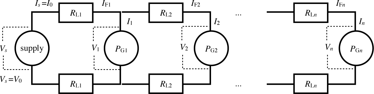
The problem becomes worse with a two-node network, as shown in Figure 2, where:
Therefore, unless I1 and I2 are known (by measurement), it has not been possible to solve for the transmission loss systematically.
1.2. Recursive Solution
Our approach is to first derive a closed-form solution to the current for a single node modeled as one power load with two transmission-line resistors. The single-node network has a closed-form solution based on the quadratic formula, and additional nodes can be viewed as additional single-node networks. Second, we extend the solution to a locally daisy-chained (LDC) network topology, which can be viewed as attaching additional stages to the previous stage to the same voltage rails as the power load, as shown in Figure 2. Third, we generalize the daisy-chained solution to tree topology by pre-order traversal. Each node applies the quadratic formula to determine the voltage across its load, which is then used as the apparent supply voltage to its children. The cumulative current drawn by the subsequent LDC stages or tree levels (commonly referred to as descendants) is solved by a recursive algorithm based on the initially estimated voltage. However, additional load by the descendants will incur a voltage drop to the power load, causing even more current to be drawn, thereby lowering the voltage across the power load. Then, the recursive solution is invoked to update the cumulative current drawn by the descendants until the whole circuit converges. Because the current drawn by each stage of the LDC or each subtree is known, the power-transmission loss can then be calculated for each transmission link accordingly.
2. Related Work
In recent year, low-power DC distribution has received growing interest due to the development of high-efficiency power converters and emerging renewable DC energy sources. Several studies have surveyed the use of low-voltage DC-power distribution. Telecommunication system commonly use 48 VDC, but as computers were introduced inside such equipment, they suffer from inefficiency, due to very high load currents. To overcome this problem, a 270-VDC power system was introduced [1], where results showed it to be superior to AC and 48-VDC systems. However, the efficiency gained in transmission due to the high voltage represents a great mismatch with the low voltage requirements of the components and peripherals in the system, making it impractical if not also hazardous and costly.
For this reason, high-voltage DC systems often fail to provide adequate performance for new generations of low-power electronic equipment, such as IP telephones, access points, switching hubs, network cameras, etc., in residential and commercial buildings [2]. To save the wiring and installation cost, power over Ethernet (PoE) was developed [3]. Although daisy-chained connection is possible though PoE, the standard only prescribes the power on point-to-point connection (e.g., via a CAT 5/5e cable up to 100 m), and thus, the use of PoE in real-world settings is limited. For example, if multiple PoE devices are daisy-chained by a 50-m cable per segment, in practice, only a few devices can be so connected, due to power-transmission loss.
Hybrid electric vehicles (HEV) use an electric propulsion system that requires over 270 V of high DC voltage [4,5] for steering, electric motors and electric machines with associated converters. However, other low-power loads, such as doors, sensors, displays, navigation computers, security, control panel, etc., are powered by a 12-V (or 24-V) car battery. Furthermore, the low-voltage loads are controlled by a controller area network (CAN), which can connect up to 100 loads in a daisy-chain within 30 m at 1 Mbps. To reduce cable weight and enable quick installation, the data lines of CAN bus tend to be combined into a power line; that is, PoCAN [6,7]. Therefore, although the CAN protocol theoretically supports up to 100 nodes in a daisy-chained topology, the number of possible connected nodes is also limited by the voltage of a power source. However, PoCAN emphasizes only the scalability of the CAN data bus without qualifying the scalability of the DC power lines. Since the number of low-power loads is increasing in vehicular applications, the number of loads that can be connected by the PoCAN line powered by the 12-V battery system is becoming an important design criterion.
Previous work on a DC-power distribution system covered AC vs. DC distribution [8,9], DC power distribution for micro power grids such as residential applications [10,11], constant power load modeling [12], fault protection [13], and stability analysis [14,15].
For long distance transmission or distribution, renewable DC power sources (e.g., solar, fuel cell) are usually converted into AC power [8,9] to be compatible with existing electrical systems. However, this AC/DC conversion incurs overhead due to harmonics, conversion loss, increases in dimension, and costs and degradation of the power quality.
To minimize overhead, DC-power distribution of renewable energy for residential places has been suggested [10,11]. The voltage level is generally 12 or 24 V for residential applications, without converting to 110–220 V AC power. This can increase power efficiency, as well as the safety of human life. However, the relatively low voltage may result in higher power loss due to cable resistance.
Unfortunately, no analytical solutions have been published on daisy-chained or tree topologies powered by a single voltage source with DC power transmission loss. This study presents a recursive algorithm that solves the current on each transmission-line segment in response to the given supply voltage. Our tool is expected to be useful for designers to check the feasibility of their system before deployment.
3. Problem Statement
The problem is to determine the transmission loss of each segment of a daisy-chained DC power network in a steady-state operating condition. The assumption implies that only stationary characteristics need to be considered during the network analysis. Since P = V×I = I2R and the line resistance of each segment is assumed to be a given constant, the problem is equivalent to solving for the Ii of each segment i. The given values are:
Vs, the supply voltage at one end of the daisy chain,
RLi, the line resistance of segment i, for i in 1…n,
PGi, the power consumption of each node i.
We assume that the power supply is either regulated or is sufficiently powerful, so that it will maintain Vs at a constant level. In the case of a battery, we assume that the internal resistance is low or can be modeled as part of RL1. We also assume that each load node is powered by a (switching) regulator, so that it responds to its (variable) supply voltage by varying its current draw to make up the load PGi. This means the equivalent resistance RGi is not a constant, but is a function of Vs at a constant level. We also assume that each load node is powered by a regulator, so that it will vary its current draw in order to maintain the given power level PGi of the load.
Note that we assume that the regulator is 100% efficient for the purposes of determining the boundary cases or feasibility. One common scenario is that the transmission loss causes so much voltage drop, that even ideal regulators cannot output any power at 0 V, making the specific configuration infeasible. Besides, when determining the load, the user is likely to measure the system empirically, so that it already takes the regulator efficiency into account. The same can be said about the supply-side regulator, too. Our measurement results actually confirm this assumption.
4. Solution
As suggested in the Introduction, formulating this problem as a classic resistive network is not productive, due to the lack of a closed-form solution for more than one node in a daisy chain or in a tree. Instead, our approach is to start with the solution of a single transmission line powering a single node at stage i (∈ [1, n]), which does have a closed-form solution based on the quadratic formula. The single-node solution to stage i of a daisy chain is used as the initial condition for the subsequent (n–i) stages, which are solved recursively to obtain the additional current draw. Then, the currents are summed to further lower the voltage input to stage i. This process is iterated until the solution converges. We first describe the single-node solution and the recursive solution. The solution to the LDC topology is then generalized to trees by following a multi-way recursive structure.
4.1. One-Node Case
In the case of one node 1, as shown in Figure 1, given Vs, PG1, RL1, the problem is to solve for I1 = IL1 = Is and, therefore, the power-transmission loss.
multiply through by Is and rearrange,
Recall that the quadratic formula a2x + bx + c = 0 has the closed-form solutions
Therefore, Is can be solved by the quadratic formula,
The physical meaning of the two solutions is that there can be two ways of achieving the same power level: a higher V with a lower I and a lower V with a higher I. However, in practice, only the smaller solution (i.e., the minus sign in ±) is realistic, because it is lower power and reached first. Besides, it is also the more stable configuration [15]. The only other consideration is that when RL1 = 0, the transmission loss is zero, and Is is due entirely to PG1/Vs. Therefore, the unique closed-form solution is:
4.2. Locally Daisy-Chained (LDC) Topology
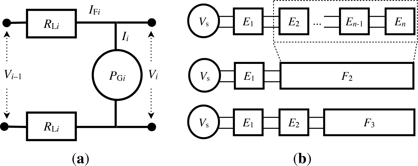
To extend this network to two or more nodes in a daisy chain, we organize the circuit as connected stages of sub-circuits, as shown in Figure 2. It is useful to take two sub-circuit views. Figure 3a shows that each stage i, called Ei (for the “i-th element”), consists of the two line resistors RLi (for the supply and ground rails) and the power consumer at PGi. It assumes that the supply has a perceived supply voltage of Vi−1 from the previous stage. To the next stage, it provides the perceived supply voltage of Vi, which is shared with the target load of this stage. Figure 3b shows the grouping of sub-circuits. i is defined to be the concatenation of Ei and i + 1, and n = En. In other words, i is the concatenation of circuits Ei …En, and therefore, 1 is the entire daisy chain. The notation for the current consumption is Ii for Ei and IFi for i, respectively.
The current consumed by i is the sum of those of Ei and i + 1. That is,
We can solve for E1 using the closed-form solution, because its input voltage is known. This enables E1 to provide V1 as the “supply” voltage to 2. However, E1 and 2 (and more generally, Ei and i + 1) are not two independent circuits, but they are parts of one circuit and interact with each other. As 2 is turned on, it will pull down the voltage seen by E1’s load, causing E1 to draw more current and lower the V1. These two sub-circuits will continue drawing additional current, but by a smaller amount over time. Eventually, the circuit will stabilize or at least hover about some sustainable level. This will happen because, in the last stage, n = En, and there is no more load beyond that point, i.e., n + 1 does not exist, and therefore, En converges as long as Vn−1 is given.
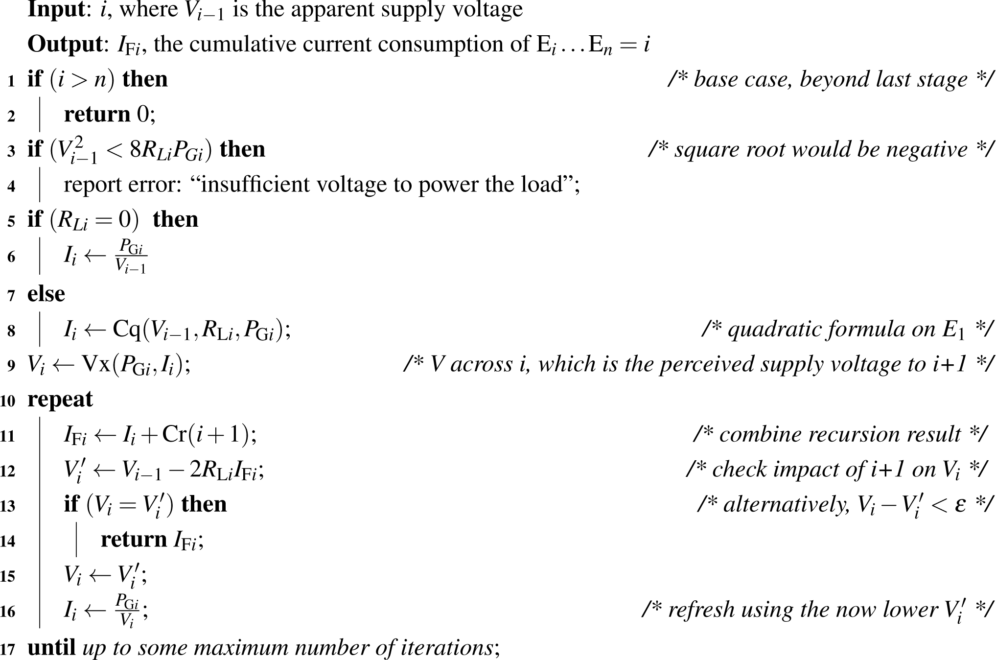
Our approach is to start with the initial solution as two independent circuits and iteratively update the load of one sub-circuit caused by the drop in supply voltage as perceived by the other sub-circuit. The pseudocode of the algorithm is shown in Algorithm 1. The current drawn by 1 (namely the entire circuit) depends on Vs. Recursively, the current drawn by sub-circuit Ei depends on Vi−1.
(Lines 1–2): Base case of recursion. If the daisy chain being considered is empty (including beyond the last stage), then it consumes no current.
(Lines 3–4) Before evaluating the quadratic formula, make sure that we are not taking the square root of a negative number, which happens when the voltage is too low (and the transmission loss is so great), such that it cannot power the entire daisy chain. In this case, the algorithm notifies the user that no feasible solution can be found for the given network.
(Lines 5–6) Another boundary case is that if RLi = 0, then there is no transmission loss, and the current Ii is due entirely to the load, namely PGi/Vi−1. The execution continues.
(Line 8) In the normal case, Ii has the quadratic formula solution to the current consumed by sub-circuit Ei:
(Line 9) With known Ii and Vi−1, we can solve for Vi to estimate the supply voltage for the next sub-circuit Ei+1.
(Line 11, Cr() call) Given Vi, we can recursively solve the current IFi+ 1 for the rest of the cumulative sub-circuit i+1. If there is no next stage (Line 2), then it is the base case and IFi+ 1 is simply zero, so IFi has a closed-form solution. We can use it to derive the power consumed by i+1.
(Line 11 + assignment) We can add the current drawn by Ei and i+1 to derive IFi ← Ii + IFi+1, where IFi+1 is solved recursively based on a snapshot of Vi. Any changes to Vi assumptions will be fixed in a later iteration.
(Line 12) We figure out the revised due to the additional voltage drop over the two RLi’s.
(Lines 13–14) If = Vi, then this means Ei and i+1 have converged to the same voltage, as neither is drawing any more incremental current.
(Line 15) Otherwise, must be lower now, so we update the current on both Ei and i+1.
(Line 16) We know that given Vi, Ii = PGi/Vi, and we will try to use Ii and IFi+ 1 to derive Vi−1.
Iterate.
4.3. Tree Topology
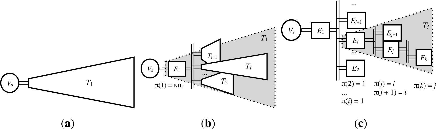
We now extend the solution to a tree topology. It entails mapping the concepts of a stage in an LDC to a node in a tree. The “car-cdr” recursive order in the style of the Lisp language on the LDC is generalized to pre-order traversal on the tree (i.e., root first, followed by its children recursively).
We organize the circuit as a tree of sub-circuits, as shown in Figure 4. Each node in the tree is a sub-circuit called Ei (for the “i-th element”), same as that in the LDC shown in Figure 3a earlier. It consists of the two line resistors RLi (for the supply and ground rails) connecting the node as a power consumer of PGi to its parent node π(i). Node i has a perceived supply voltage of Vπ(i) from its parent before the transmission line.
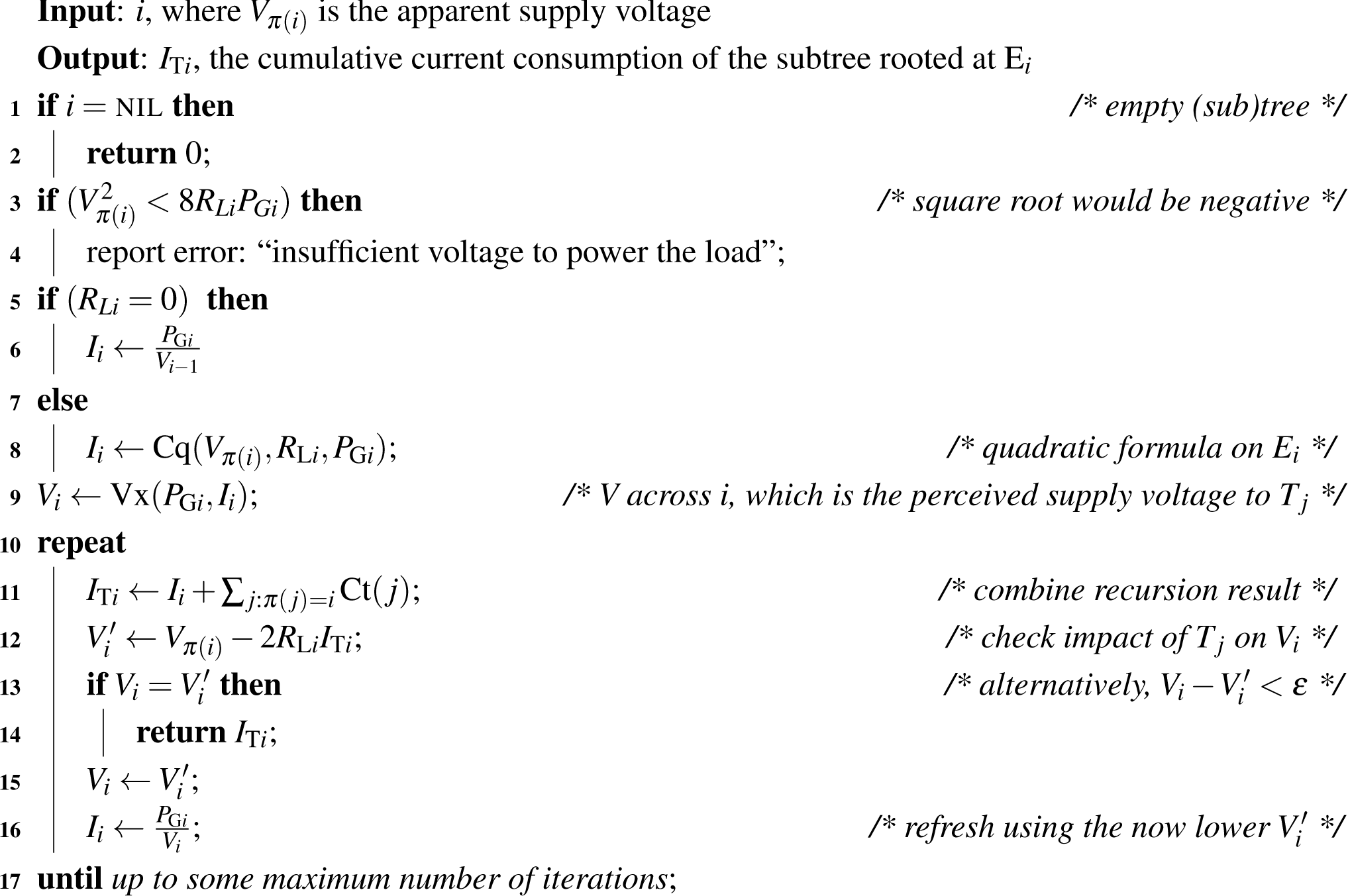
A node i in the tree can have zero or more children. The subtree rooted at i is denoted Ti, which is defined as the joining of sub-circuits Ei and its children subtrees Tj for all j: π(j) = i. T1 is the entire tree, as shown in Figure 4a, and Figure 4b shows the partially expanded view. More generally, Figure 4c shows how a tree can be further expanded in more detail. If node i is called a leaf, if ∄j: π(j) = i, in which case Ti = Ei. To its children, node i provides the common perceived supply voltage of Vi, which is shared with the load PGi. The notation for the current consumption is Ii for Ei and ITi for Ti, respectively. The current consumed by Ti is the sum of those of Ei and Tj∀j: π(j) = i. That is,
The algorithm for the tree follows the same general structure as that for the LDC. For each subtree starting with i = 1, we can solve for Ei using the closed-form solution, because its input voltage is known. This enables Ei to provide Vi as the “supply” voltage to its children Tj’s. However, Ei and Tj’s are not independent circuits, but they are parts of one circuit and interact with each other. As each Tj is turned on, it will pull down the voltage seen by Ei’s load, causing Ei to draw more current and lower the Vi. These sub-circuits will continue pulling more current each time, but by a smaller amount, and eventually converge to a sustainable level. Similar to the last stage of an LDC, for all leaf nodes, Ti = Ei, and ∄j: π(j) = i, and therefore, Ei will converge by definition, as long as Vπ(i) is given.
The pseudocode of the algorithm is shown in Algorithm 2. The current drawn by T1 (namely the entire circuit) depends on Vs. Recursively, the current drawn by sub-circuit Ei depends on Vπ(i).

(Lines 1–2) Base case of recursion. If the tree being considered is empty, then it consumes no current.
(Lines 3–6) Catch the infeasible case before taking the square root of a negative number, and skip division by zero if the line resistance is zero.
(Line 8) If Vπ(i) is known, then Ii has same quadratic formula solution (i.e., Equation (9)) to current consumed by sub-circuit Ei.
(Line 9) With known Ii and Vπ(i), we can solve for Vi to estimate the supply voltage for the next-level sub-circuits Tj∀j: π(j) = i.
(Line 11, Ct() call) Given Vi, we can recursively solve the current ITj for the children cumulative sub-circuits Tj. If it has no children (i.e., ∄j), the empty summation ∑j:π(j)=i Ct(j) is simply zero, so ITi has a closed-form solution. We can use it to derive the power consumed by Tj.
(Line 11 + assignment) We can add the current drawn by Ei and Tj to derive ITi ← Ii +∑j:π(j)=i ITj, where ITj is solved recursively based on a snapshot of Vi. Any changes to Vi assumptions will be fixed in a later iteration.
(Line 12) We figure out the revised due to the additional voltage drop over the two RLi’s.
(Lines 13–14) If , then the power consumption of Ti has converged.
(Line 15) Otherwise, the power still has not converged, and must be lower now, so we update the current on both Ei and all children Tj.
(Line 16) We know that if given Vi, then Ii = PGi/Vi, and we will try to use Ii and ITj to derive Vπ(i).
Iterate.
5. Execution Trace
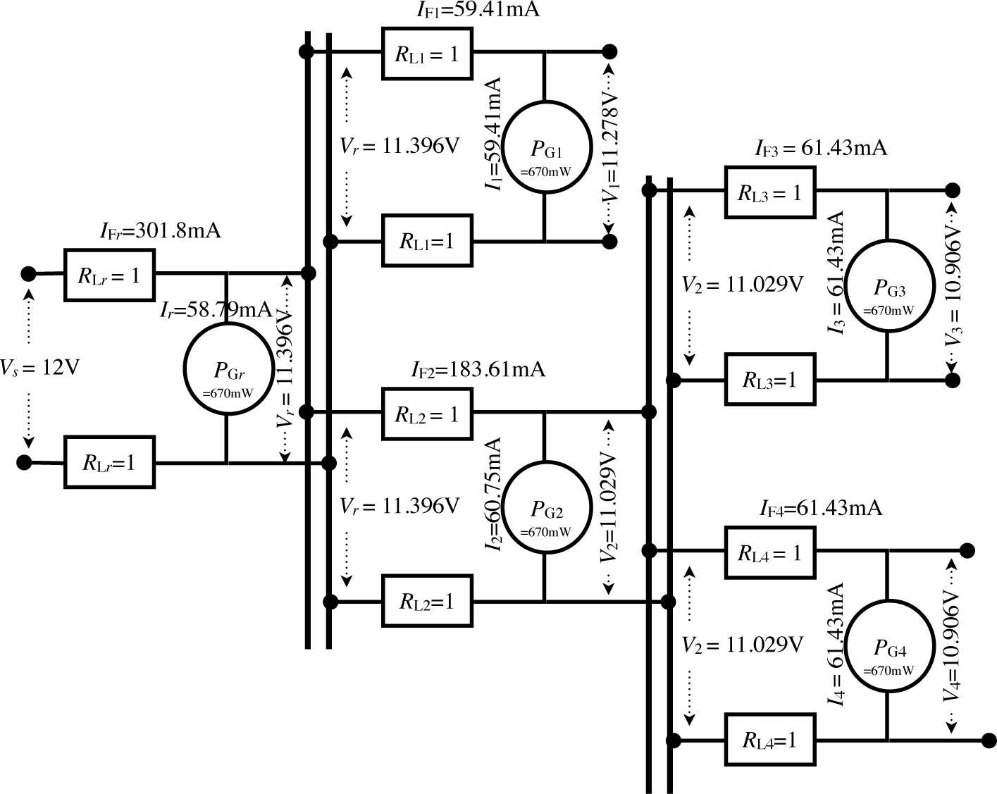
We have swept the supply voltage for a tree circuit in Figure 5 from 18 V down to 6 V, based on commonly-available battery technologies. Common car batteries (e.g., 40 Ah) are typically 12 V, while high-capacity (e.g., 600 Ah) marine batteries are 6 V. Table 1 shows the supply voltage, total current consumption, total power consumption and total power-transmission loss of the same network. Even though the total net load remains constant (3.35 W), the power-transmission loss goes from 109.7 mW at 18 V up to 1.46 W at 7 V, or over 13 times as much. When the supply voltage drops down to 6 V and below, the loss is so high, that it fails to power the entire network, no matter how large the battery capacity may be. This example shows that our algorithm can be used for design-space exploration of not only different supply voltages, but also the cable quality and topology.
To help illustrate the execution of our algorithm, let us consider the example in Figure 5. Because Ct() is a recursive algorithm, we use the indentation level to indicate the level of nesting of invoking the Ct() function during its execution.
The user calls Ct(r) with Vs = 12.
Line 1 checks the base case and skips Line 2, because r (the root) is not NIL.
Lines 3–6 ensure no overload condition or zero line resistance.
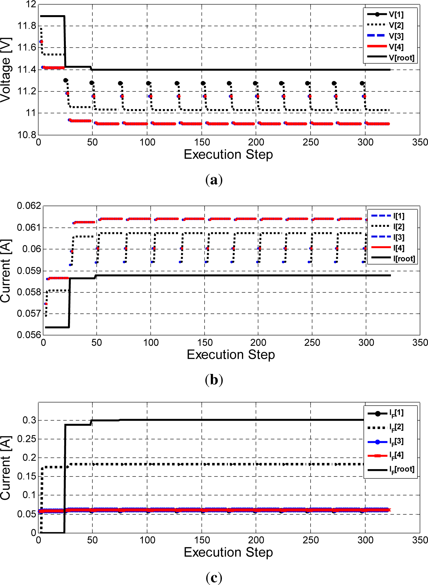
Line 8 applies the quadratic formula, and Line 9 calculates the corresponding voltage. We get Ir = 0.056363 and Vr = 11.887274 at this point.
The algorithm enters a loop to recursively compute the total current drawn by its two subtrees, 1 and 2.
– Calling Ct(1) on subtree i = 1:
* Here, π(1) is the root, so Vπ(i) = Vr = 11.887. As the base cases do not apply, Lines 8 and 9 yield V1 = 11.773 and I1 = 0.056908.
* In the loop, Line 11 attempts to recursively call all of Node 1’s children (i.e., those nodes j whose predecessor π(j) is one. However, since no such nodes exist, IT1 simply gets a copy of I1 with a trivial summation.
* Line 12 refreshes the voltage drop by two line resistors RL1 using the new current from its subtrees.
* Line 13 checks if Subtree 1’s voltage has converged. Since the line resistors are being considered for the very first time on the previous line, they pull down the voltage, so the voltage has not converged.
* Lines 15 and 16 refresh the voltage and current by considering the load PG1, and we get V1 = 11.773459, I1 = 0.056908, while IF1 remains unchanged at 0.056908.
* The algorithm runs for an additional iteration and converges, returning its IF1 value to Ct(r), which is just receiving the result for its first summation term.
– Calling Ct(2) on subtree i = 2:
* This is similar to Subtree 1, except that Subtree 2 has children. Therefore, after the quadratic formula on Load 2, the current summation on Line 11 results in two recursive calls to Ct(3) and Ct(4). Both are leaf nodes and apply the quadratic formula without further recursive calls. After the first iteration, they yield V3 = V4 = 11.658522, I3 = I3 = 0.057469 and IF3 = IF4 = 0.057469, since both subtrees have identical line resistance and load.
* In our implementation, Ct(2) converges after nine iterations. Since V3 =V4 = 11.419078, I3 = I4 = 0.058674, IF3 = IF4 = 0.058674, we get V2 = 11.536426, I2 = 0.058077, IF2 = 0.175424.
By the end of Ct(r)’s first iteration, we have Vr = 11.422610, Ir = 0.058656, IFr = 0.288695.
Ct(r) resumes its loop for a total of 11 more iterations before Vr converges.
Figure 6 plots the values of Vi;Ii and IFi over the execution steps of the algorithm in the three charts.
6. Validation
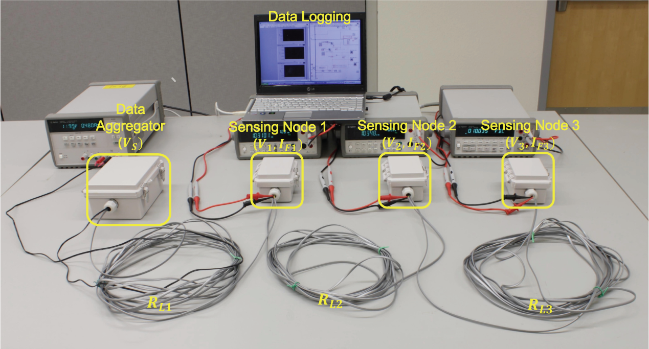
We validated our algorithm by measurement on a real-life, daisy-chained water-pipe monitoring system, called DuraMote [16]. Our validation setup consists of one data aggregator and three daisy-chained sensing nodes, as shown in Figure 7. Adjacent nodes are connected via a 10-m phone cable (RJ9) with four wires of RLi = 1 Ω each, including one for supply, one for ground and two for CAN data. Assuming static voltage is directly supplied to each sensing node by either utility power or energy buffer, the total power consumption (Pstatic) of three sensing nodes is 4.86 W (=1.62 W×3) in active mode and 47.1 mW (=15.7 mW×3) in sleep mode. Table 2 shows the voltage, current and power-transmission loss as measured by the setup shown in Figure 7 and calculated by our Cr() algorithm over a 12-V supply voltage at each LDC segment in active mode. With a supply voltage of 12 V and three identical sensing nodes, the measurement results in an active mode match within 0.1% of the computed current.
7. Conclusions
This article presents an algorithm for solving the power loss in DC transmission networks. We believe that this is the first general solution proposed for this fundamental problem in electrical engineering. The base case of our recursive algorithm has a closed-form solution for a single node based on the quadratic formula. The recursive case and the base case decrease each other’s perceived supply voltage until they converge. We first derive a solution for a daisy-chained topology and extend it to a tree topology. In practice, the solution converges very quickly (much less than one second). This solution can be valuable for exploring trade-offs among power loss, cost and other considerations, especially in low-voltage DC-powered networks.
Future work includes more general models of the circuit. Specifically, for now, we consider symmetric line resistance on the supply path and ground path, but that is not necessarily the case. Another direction is the extension to circuits with cycles, that is multiple paths from the supply to a given node. Some problems contain properties of both. For instance, automobiles commonly use the car body as the ground, making it more difficult to predict the resistance of the ground path. It is certainly an asymmetric supply/ground problem, because the supply lines are separate, whereas the ground lines are tied together; moreover, it is also a cyclic problem, because all ground lines can be viewed as being connected to each other in a clique. We believe that the solution here can serve as a basis on which these other problems can be solved.
Acknowledgments
The present research was supported by the research fund of Dankook University in 2014.
Author Contributions
Dr. Kim designed and validated the recursive algorithms. As the first author, he has analyzed the pertinent acquired data on which the results and conclusions of this study are based. Dr. Chou wrote the majority of the original draft of the article. As a corresponding author, he guarantees that all individuals who meet the authorship criteria are included as authors of this paper.
Conflicts of Interest
The authors declare no conflict of interest.
References
- Yamashita, T.; Muroyama, S.; Furubo, S.; Ohtsu, S. 270 VDC system—A highly efficient and reliable power supply system for both telecom and datacom system, Proceedings of the IEEE International on Telecommunication Energy Conference, Copenhagen, Denmark, 6–9 June 1999.
- Marquet, D.; San Miguel, F.; Deshayes, A.; Tetart, J.-C. New power supply optimised for new telecom networks and services, Proceedings of the IEEE International on Telecommunication Energy Conference, Copenhagen, Denmark, 6–9, June 1999.
- IEEE Std 802.3at-2009 (Amendment to IEEE Std 802.3-2008); IEEE Xplore Digital Library, 2009. Available online: http://ieeexplore.ieee.org/stamp/stamp.jsp?tp=&arnumber=5306743 accessed on 13 November 2014.
- Chan, C.C. An overview of electric vehicle technology. Proc. IEEE 1995, 81, 1202–1213. [Google Scholar]
- Chan, C.C. The state of the art of electric and hybrid vehicles. Proc. IEEE 2002, 90, 247–275. [Google Scholar]
- Beikirch, H.; Vo., M. CAN-Transceiver for field bus powerline communications, Proceedings of the International Symposium on Power Line Communications and Its Application, Limerick, Ireland, 5–7 April 2000; 90, pp. 257–264.
- Shinozuka, M.; Chou, P.H.; Kim, S.; Kim, H.R.; Pul, S. Nondestructive monitoring of a pipe network using a MEMS-based wireless network, Proceedings of the Nondestructive Characterization for Composite Materials, Aerospace Engineering, Civil Infrastructure, and Homeland Security IV, San Diego, CA, USA, 9 March 2010.
- Starke, M.; Tolbert, L.M.; Ozpineci, B. AC vs. DC distribution: A loss comparison, Proceedings of the Transmission and Distribution Conference and Exposition, Chicago, IL USA, 21–24 April 2008; pp. 1–7.
- Justo, J.J.; Mwasilu, F.; Lee, J.; Jung, J.-W. AC-microgrids versus DC-microgrids with distributed energy resources: A review. Renew. Sustain. Energy Rev 2013, 24, 387–405. [Google Scholar]
- Kakigano, H.; Miura, Y.; Ise, T. Low-voltage bipolar-type DC microgrid for super high quality distribution. J. IEEE Trans. Power Electron 2010, 25, 3066–3075. [Google Scholar]
- Cetin, E.; Yilanci, A.; Ozturk, H.K.; Kasikci, I.; Colak, M.; Icli, S. Construction of a fuel cell system with DC power distribution for residential applications. Int. J. Hydrog. Energy 2011, 36, 11474–11479. [Google Scholar]
- Salomonsson, D.; Sannino, A. Load modelling for steady-state and transient analysis of low-voltage DC systems. J. Electr. Power Appl. IET 2007, 1, 690–696. [Google Scholar]
- Cairoli, P.; Kondratiev, I.; Dougal, R. Ground fault protection for DC bus using controlled power sequencing, Proceedings of the IEEE SoutheastCon 2010, Concord, NC, USA, 18–21 March 2010; pp. 234–237.
- Bellthayat, M.; Cooley, R.; Witulski, A. Large signal stability criteria for distributed systems with constant power loads, Proceedings of the 26th Annual IEEE on Power Electronics Specialists Conference, Atlanta, GA, USA, 18–22 June 1995; 2, pp. 1333–1338.
- Karlsson, P.; Svensson, J. DC bus voltage control for a distributed power system. J. IEEE Trans. Power Electron 2003, 18, 1405–1412. [Google Scholar]
- Kim, S.; Torbol, M.; Chou, P.H. Remote structural health monitoring systems for next generation SCADA. Smart Struct. Syst 2013, 11, 511–531. [Google Scholar]


| Execution items | Execution trace over the swept supply voltage from 6 V to 18 V | |||||||
|---|---|---|---|---|---|---|---|---|
| voltage | 18 V | 15 V | 12 V | 10 V | 9 V | 8 V | 7 V | 6 V |
| total current | 192.21 mA | 234.21 mA | 301.81 mA | 377.77 mA | 435.71 mA | 522.09 mA | 687.09 mA | infeasible |
| total power | 3.46 W | 3.51 W | 3.62 W | 3.78 W | 3.92 W | 4.18 W | 4.81W | - |
| power-transmission loss | 109.70 mW | 163.14 mW | 271.77 mW | 427.73 mW | 571.42 mW | 826.71 mW | 1.46 W | - |
| Mode | Segment, i | Sensing Node 1 | Sensing Node 2 | Sensing Node 3 | |||
|---|---|---|---|---|---|---|---|
| Measured | Computed | Measured | Computed | Measured | Computed | ||
| Active | voltage (Vi) | 11.08 V | 11.08 V | 10.45 V | 10.45 V | 10.13 V | 10.13 V |
| current (IFi) | 461.2 mA | 461.27 mA | 315.1 mA | 315.02 mA | 159.9 mA | 159.96 mA | |
| power-trans. loss | 425.41 mW | 425.53 mW | 198.58 mW | 198.48 mW | 51.16 mW | 51.17 mW | |
© 2014 by the authors; licensee MDPI, Basel, Switzerland This article is an open access article distributed under the terms and conditions of the Creative Commons Attribution license (http://creativecommons.org/licenses/by/4.0/).
Share and Cite
Kim, S.; Chou, P.H. A Recursive Solution for Power-Transmission Loss in DC-Powered Networks. Energies 2014, 7, 7519-7534. https://doi.org/10.3390/en7117519
Kim S, Chou PH. A Recursive Solution for Power-Transmission Loss in DC-Powered Networks. Energies. 2014; 7(11):7519-7534. https://doi.org/10.3390/en7117519
Chicago/Turabian StyleKim, Sehwan, and Pai H. Chou. 2014. "A Recursive Solution for Power-Transmission Loss in DC-Powered Networks" Energies 7, no. 11: 7519-7534. https://doi.org/10.3390/en7117519