Analysis of Future Vehicle Energy Demand in China Based on a Gompertz Function Method and Computable General Equilibrium Model

Abstract

This paper presents a model for the projection of Chinese vehicle stocks and road vehicle energy demand through 2050 based on low-, medium-, and high-growth scenarios. To derive a gross-domestic product (GDP)-dependent Gompertz function, Chinese GDP is estimated using a recursive dynamic Computable General Equilibrium (CGE) model. The Gompertz function is estimated using historical data on vehicle development trends in North America, Pacific Rim and Europe to overcome the problem of insufficient long-running data on Chinese vehicle ownership. Results indicate that the number of projected vehicle stocks for 2050 is 300, 455 and 463 million for low-, medium-, and high-growth scenarios respectively. Furthermore, the growth in China’s vehicle stock will increase beyond the inflection point of Gompertz curve by 2020, but will not reach saturation point during the period 2014–2050. Of major road vehicle categories, cars are the largest energy consumers, followed by trucks and buses. Growth in Chinese vehicle demand is primarily determined by per capita GDP. Vehicle saturation levels solely influence the shape of the Gompertz curve and population growth weakly affects vehicle demand. Projected total energy consumption of road vehicles in 2050 is 380, 575 and 586 million tonnes of oil equivalent for each scenario.

1. Introduction

Due to the large size of and tremendous growth in the Chinese automotive market, forecasting the development trend of China’s vehicle fleet is important for academic researchers as well as policymakers in the fields of sustainable mobility and environmental protection.

Firstly, fossil fuels are the most important primary energy source in most countries around the world and the transportation sector, particularly individual transport, is highly dependent on fossil fuels [1]. There is strong demand for oil because of increasing private vehicle ownership [2]. China is also facing energy supply problems due to limited fossil energy resources. Its per capita reserves of coal, petroleum and natural gas (NG) are 67.0%, 5.4%, and 7.5% of world average reserves, respectively [3]. Furthermore, as Organization for Economic Co-operation and Development (OECD) oil use declines, China will become the largest consumer of oil by 2030s and Chinese demand is concentrated in transport [4].

Secondly, vehicle emissions are the dominant source of air pollution and the transportation sector accounts for a large fraction of air pollution emissions [5,6,7]. According to the International Maritime Organization’s second Greenhouse Gas (GHG) study [8] the highest CO₂ emitting transport mode is road, which contributes 21.3% of the CO₂ emitted globally and is second only to electricity and heat production which contributes 35%. Because of the overwhelming use of petroleum as the fuel of choice, Gao and Winfield [9] further note that road vehicles not only reduce petroleum resources but also release a significant amount of exhaust fumes which contribute to global warming and harm the environment and human health.

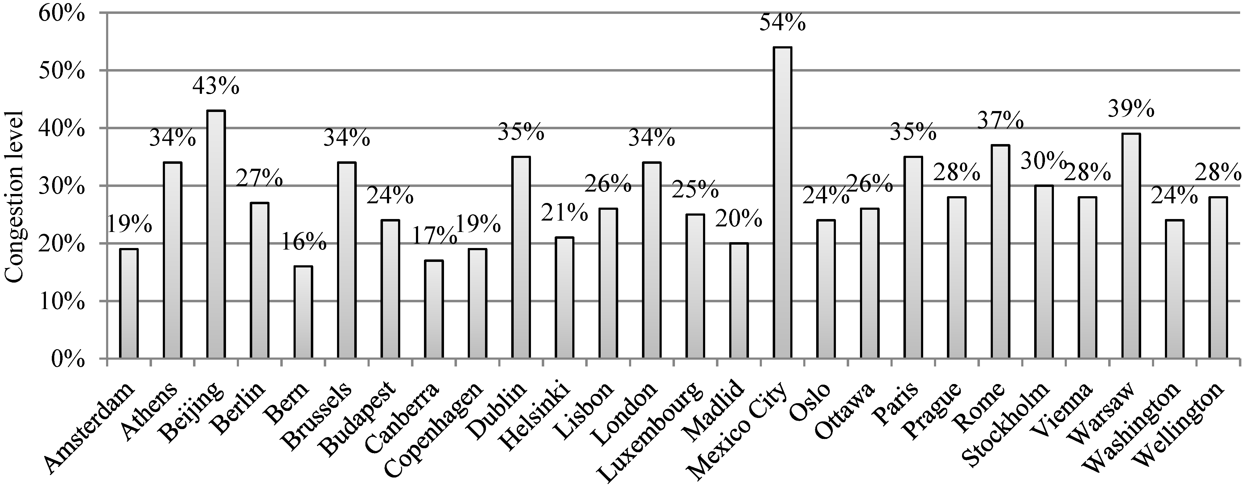
Thirdly, the fast growth in vehicle ownership has caused concerns over traffic congestion, especially in large Chinese cities [10]. In the urban areas of China, the rapid growth in traffic has led to severe congestion problems and particularly a lack of parking space [11]. According to the reports by TomTom Traffic Index [12], China’s congestion level in 2013 was 36%, exceeding levels in Europe (26%), Australia & New Zealand (26%) and the Americas (20%). The congestion level in Beijing far exceeds congestion levels in all other capital cities within Organization for Economic Co-operation and Development (OECD) countries, with the exception of Mexico City (see Figure 1).

Finally, the automotive industry is one of the largest sectors in the global market and the automobile is an increasingly technology intensive product [13]. The growth rate of China’s car market has accelerated rapidly over the past two decades [14]. In China, the production and sales of vehicles exceeded 20 million units in 2013 and China has had the highest vehicle production and vehicle sales in the world for five consecutive years [15]. According to projections by Huo et al. [16], total vehicle stock in China will exceed that of the U.S. within 15 years.

Figure 1. Congestion levels in capital cities in 2013 (data source: [12]). All founding members of OECD are included, excepting Iceland and Turkey, because of lack of data.

Figure 1. Congestion levels in capital cities in 2013 (data source: [12]). All founding members of OECD are included, excepting Iceland and Turkey, because of lack of data.

It is standard practice in the vehicle forecast literature to model projected vehicle ownership using the Gompertz function when economic variables such as per capita income or per capita gross domestic product (GDP) are being used as the main explanatory variables. Huo and Wang [17] employ per capita income as an economic factor, while several researchers use per capita GDP on the basis of macro level [18,19,20,21,22]. Meyer et al. [23] use income data based on a micro level; moreover the authors use GDP time series from the World Bank database (World Development Indicators). Wu et al. [15] notes that GDP should be used instead of income to estimate vehicle demand in China because of biases in the reporting of Chinese income statistics and the impact of Chinese Government intervention on the balance between vehicle supply and demand. Indeed, most studies use the GDP-dependent Gompertz function to estimate Chinese vehicle stocks [15,24,25,26]. We therefore employ the GDP-dependent Gompertz function.

As Wang et al. [27] note, the first major challenge in forecasting vehicle populations using the GDP approach is the accuracy of the GDP forecasts themselves. The latest reports show that growth in China is set to slow in the post-industrial era at around 2020 [28,29] because of a “middle-income trap” referred by World Bank [30] or the characteristics of the industrialization process. The process of industrialization can be divided into three stages, consistent with Bell’s conception of post-industrialization: pre-industrialization, industrialization and post-industrialization [31]. The index of industrial production (IIP) is generally used to quantify the economic value of industrial production and indicate industrial output and activity [32]. The IIP is probably the most important and widely analyzed indicator, given the driving role played by manufacturing in the business cycle. Further, the IIP is a crucial variable used to forecast the short-run evolution of GDP in most countries [33]. 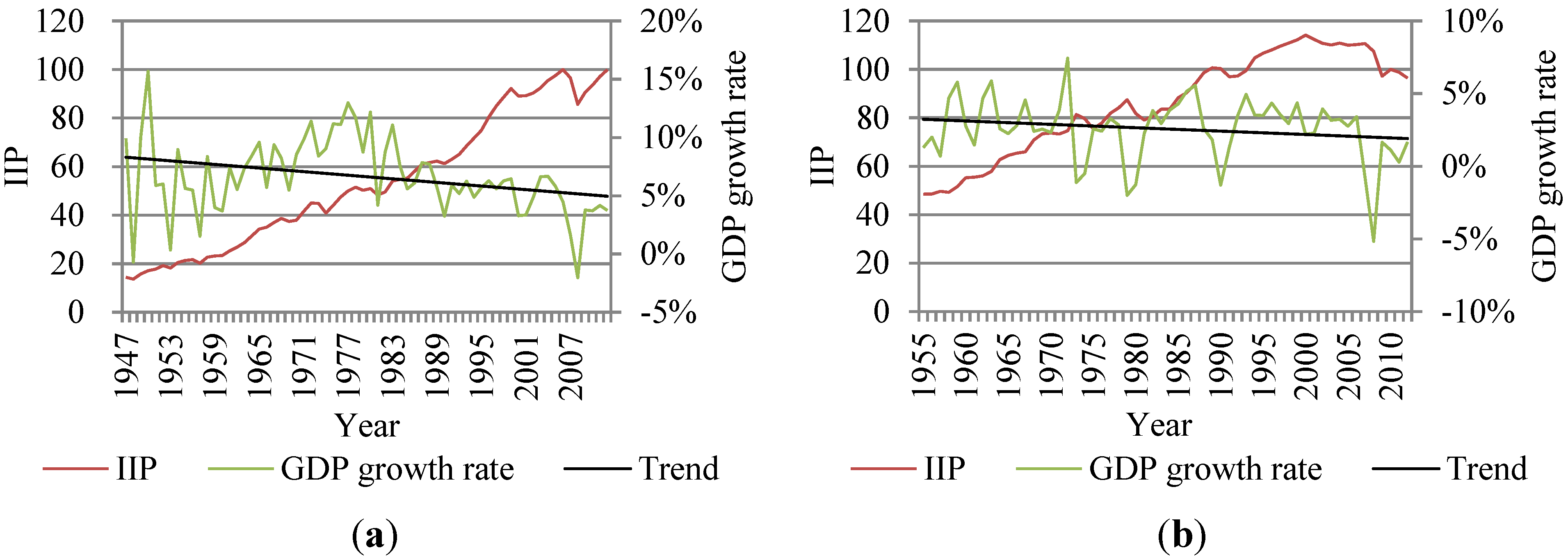Figure 2 illustrates the annual IIP and annual GDP growth rate in the United States (U.S.) and United Kingdom (UK).

Figure 2. Annual growth rate of industrial production (IIP) and gross domestic product (GDP) in the U.S. and UK (Data source: [34,35,36,37]). (a) United States (Index 2007 = 100); (b) United Kingdom (Index 2010 = 100).

Figure 2. Annual growth rate of industrial production (IIP) and gross domestic product (GDP) in the U.S. and UK (Data source: [34,35,36,37]). (a) United States (Index 2007 = 100); (b) United Kingdom (Index 2010 = 100).

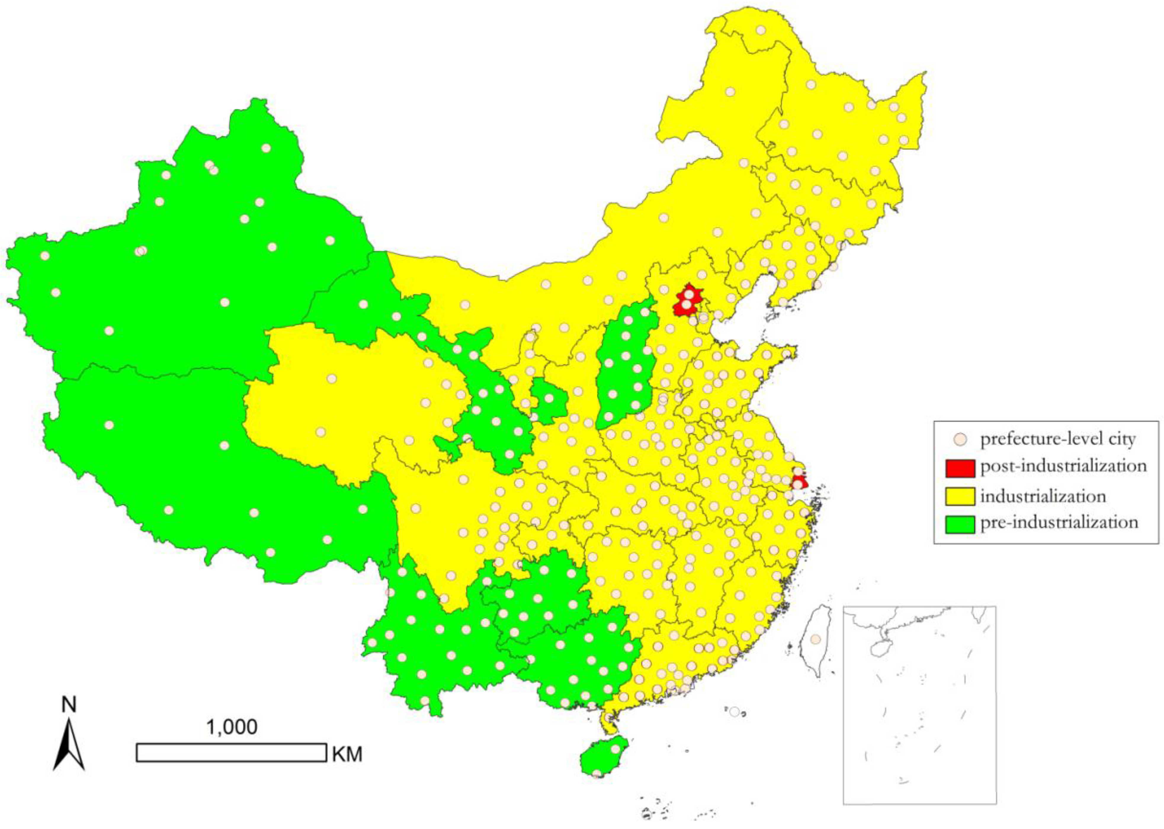
International experience shows that the growth rate of annual GDP decreases with industrialization (see Figure 2). China has not yet reached the post-industrialization stage till now, with most provinces being in the industrialization and pre-industrialization stages, with the exception of Beijing and Shanghai (see Figure 3). According to the Report of Hu Jintao to the 18th CPC (Communist Party of China) National Congress [38], industrialization should be complete by approximately 2020. We therefore expect GDP growth in China to slow over the next decade.

Figure 3. The process of industrialization across regions of China in 2010 (data source: [39]).

Figure 3. The process of industrialization across regions of China in 2010 (data source: [39]).

It is therefore necessary to obtain a detailed and full understanding of Chinese automotive developments, particularly during the transition from pre-industrialization to post-industrialization. The accuracy of GDP forecasts are especially important over this transitional period as is the impact of alternative GDP growth rates on vehicle fleet projections. In contrast to previous studies that assumed a single annual Chinese GDP growth rate [24], this paper establishes a recursive dynamic Computable General Equilibrium (CGE) model to forecast the Chinese economic growth rate from 2013 to 2050. Unlike traditional econometric methods [15], the CGE model is based on the general equilibrium theory of Walras and therefore uses a series of simultaneous equations to characterize the interdependence between different economic sectors and agents in a macroeconomic system [40]. Agents and sectors make choices to maximize their objective function, for example, utility functions for consumers and profit functions for firms. Finally, we used the model to estimate the price and resource allocation in equilibrium.

Our analysis contributes to several literature topics. Firstly, the existing Gompertz function analyses are widely used to specify dynamic features of the automotive market and to estimate the growth in vehicle ownership using economic explanatory variables. Of the three growth functions—Gompertz, Logistic and Richards—several studies have showed that the Gompertz function best fits the historical vehicle ownership data [17,18]. Secondly, this paper is directly related to previous research on projected Chinese vehicle ownership. Huo et al. [24] estimated the highway vehicle stocks from 2011 to 2050 in China based on three different growth scenarios—high-growth, medium-growth and low-growth. Wu [25] forecasted China’s vehicle stock through 2030 and projected the share of each major vehicle category, including cars, buses and trucks. The truck category is subdivided into a further four categories: heavy-duty, medium-duty, light-duty and mini trucks. Zheng et al. [26] estimated county-level vehicle ownership using the Gompertz function and observed significant spatial differences in vehicle population and ownership between Chinese counties. Furthermore, the results in Zheng et al. [26] demonstrate that economic development is highly correlated with vehicle ownership. Wu et al. [15] projected vehicle stock levels in China based on the extant patterns of vehicle development across all OECD countries, Europe, the U.S. and Japan, respectively. Their results show that the OECD and European patterns better describe the growth in China’s vehicle stock than Japanese or U.S. patterns. Thirdly, this paper also relates to the empirical literature on long-term projections of GDP growth rates. There are two broad classes of methodologies: the CGE model and, the production function method with a growth accounting framework. The CGE model is widely used in many fields such as tax reform, international trade, employment, education and energy resources. A number of CGE models have been used to estimate China’s economic growth in the next several decades [41,42,43]. We extend these analyses by forecasting a series of GDP growth rates under three possible growth scenarios.

This paper makes several important advances over the previously cited literature on Chinese vehicle ownership. Firstly, we forecast China’s annual GDP growth rate using a recursive dynamic CGE model rather than a multiple autoregressive moving average (MARMA) model. The CGE model is more general used for long-term GDP growth forecasts. Secondly, we use data for all OECD countries and estimate vehicle growth rates under three scenarios—high-growth, mid-growth and low-growth. Thirdly, by estimating vehicle populations under three growth scenarios enables us to explore the sensitivity in vehicle projections according to variations in key factors, including vehicle saturation level, GDP growth rate and population growth. This is important given the uncertainty over Chinese economic and automotive industry development. Finally, the total energy consumption of road vehicles and the fuel consumption of other major categories of vehicle are analyzed.

The paper is organized as follows. Section 2 presents the methodology, research approach and the data sources. Section 3 reports the projected annual vehicle ownership and energy demand in the transport sector in China from 2013 to 2050. This section also includes a discussion of the impact of the different key parameters (i.e., vehicle saturation level, GDP growth rate and population growth rate) on vehicle stock projections and energy consumption. Finally, Section 4 presents our conclusions and provides policy suggestions.

2. Methodology and Data

There are three factors in the Gompertz function: (a) per capita GDP; (b) the saturation level of vehicle ownership and; (c) curvature parameters [44]. Therefore, each of these parameters needs to be estimated to obtain a projection of Chinese vehicle ownership.

This study proceeds as follows. Firstly, we build a CGE model to project China’s annual GDP growth rate from which per capita GDP can be derived. Secondly, we set the ultimate saturation level of vehicle ownership for each country according to the existing literature [20]. Finally, we determine the curvature parameters. The rule of thumb stating that sample size N > 30 is sufficient for asymptotic theory to provide a good approximation for inference on a single variable does not extend to models with regresses [45]. Historical data on Chinese vehicle ownership is unavailable for a sufficiently long period, therefore the Gompertz function is estimated using data on vehicle development trends of the founding members of the OECD countries under the assumption that the OECD pattern best describes China’s vehicle stock growth, as illustrated by Wu et al. [15]). The estimated parameters are used to predict the annual vehicle ownership in China. The data before 2013 are historical, with all projections based on the historical data.

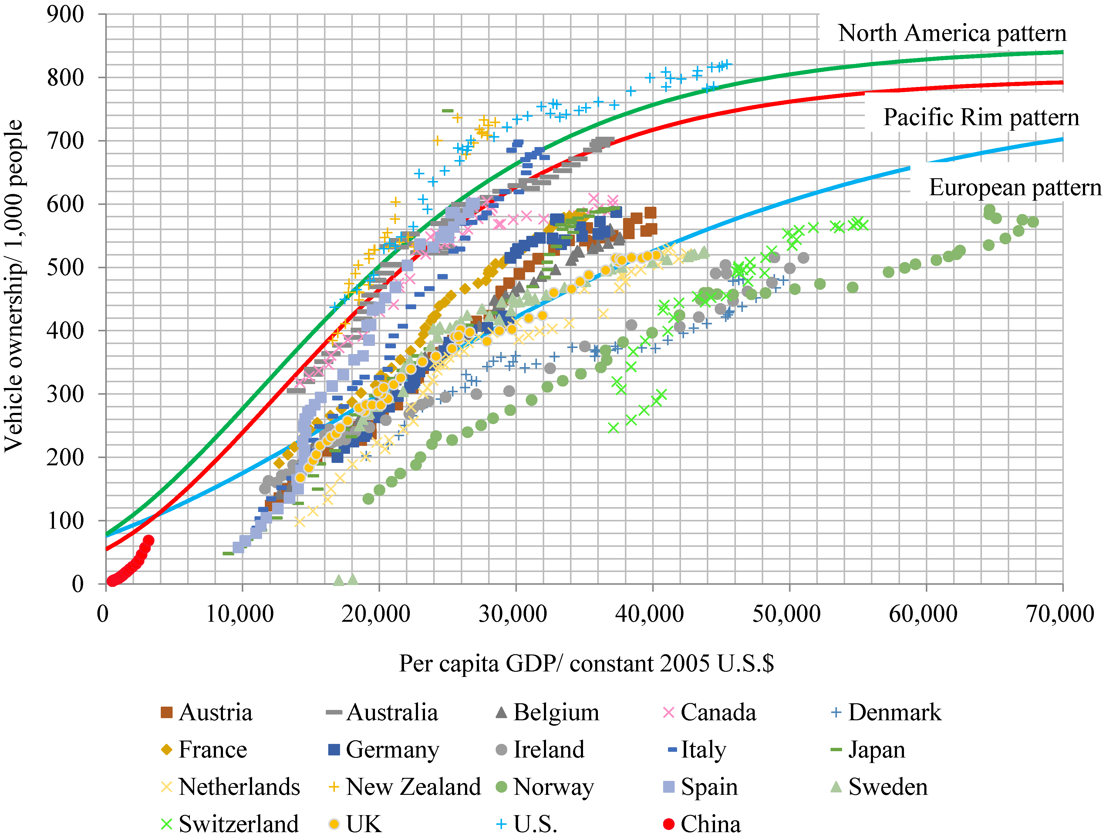
Before introducing the methodology and data, we describe the vehicle development trends across OECD countries (see Figure 4).

The Development Research Center of the State Council [46] and Huo et al. [24] divide vehicle demand growth into three periods: incubation period (with an initial slow growth period), booming period (intermediate stage of the Gompertz S-curve, covering the inflection point) and saturated growth period (the growth rate of the Gompertz S-curve is decreasing). Figure 4 shows that most OECD countries present different characteristics but closely follow the Gompertz curve. The Pacific Rim and North America patterns display the greatest curvature in the booming period and both have entered the saturated growth phase. European countries remain in the booming period, presenting rapid growth in automotive markets, but display a comparably smoother growth pattern in the intermediate stage of the Gompertz S-curve. The red circle trend line (lower left corner of the first quadrant) represents China’s current position; China has not reached the inflection point of the increasing curve and remains in the rapid growth period. Therefore, it is necessary to estimate future Chinese vehicle ownership under different growth scenarios.

Figure 4. Growth trends of vehicle stocks in representative OECD countries (data source: [47,48]).

Figure 4. Growth trends of vehicle stocks in representative OECD countries (data source: [47,48]).

2.1. Gompertz Function

The Gompertz function has been widely used to estimate vehicle ownership [15,17,18,19,20,21,22,23,24,25,26]. This study therefore follows standard econometric methodology by employing the Gompertz function to estimate vehicle ownership in China. The Gompertz function is regularly expressed as the following Equation (1):

$$V_{i,t}=V_i^{*}\times e^{\text{α}{e}^{\text{β}E{F}_{i,t}}}$$

(1)

where V_i,t represents the number of vehicles per 1000 people in country i in year t; $V_i^{*}$ is the ultimate saturation level of vehicle ownership (vehicles per 1000 people) in country i; EF_i,t is per capita GDP in country i in year t; α and β are two negative parameters that determine the shape of the S-curve in different economic levels. The parameter α determines the demands of vehicle stocks at low or zero economic levels and the parameter β is a curvature parameter that controls the slope of the Gompertz function at high economic levels.

Taking the logarithm of both sides of Equation (1), the estimating equation can be expressed as the following Equation (2):

$$\text{ln}\left(\text{ln}\frac{V_i^{*}}{V_{i,t}}\right)=\text{ln}\left(-\text{α}\right)+\text{β}E{F}_{i,t}$$

(2)

As shown as Equation (2), time-subscripts and region-subscripts are added where appropriate. Therefore, we implement panel regressions for unbalanced panel data because, for several countries, data for a sufficiently long period were unavailable.

2.2. Computable General Equilibrium (CGE) Model

The recursive dynamic CGE model in our study consists of 42 production sectors (see Table 1), four primary economic factors (productive labor, professional labor, agricultural labor, capital), four types of energy input (coal, crude oil, gas, electricity), two classes of household (rural and urban) and five basic account types (enterprise, government, investment and saving, stock, foreign).

Table 1. Sector classification in CGE model.

No.	Sector	No.	Sector
1	Agriculture, forestry, animal husbandry and fishery	22	Scrap waste
2	Coal mining and washing	23	Electricity, heat production and supply industry
3	Oil and gas exploration industry	24	Gas Production and Supply
4	Metal mining industry	25	Water production and supply industry
5	And other non-metallic mineral mining industry	26	Construction
6	Food manufacturing and tobacco processing industry	27	Transportation and Warehousing
7	Textile industry	28	Postal Services
8	Textile, leather and feather products industry	29	Information transmission, computer services and software industry
9	Wood processing and furniture manufacturing	30	Wholesale and retail trade
10	Paper printing and Educational and Sports Goods	31	Accommodation and Catering Services
11	Petroleum processing, coking and nuclear fuel processing industry	32	Financial Industry
12	Chemical Industry	33	Real Estate
13	Non-metallic mineral products industry	34	Leasing and Business Services
14	Metal smelting and rolling processing industry	35	Research and Development Industry
15	Fabricated Metal Products	36	Integrated Technical Services
16	General, special equipment manufacturing industry	37	Water conservancy, environment and public facilities management industry
17	Transportation Equipment Manufacturing	38	Resident Services and Other Services
18	Electrical machinery and equipment manufacturing	39	Education
19	Communications equipment, computers and other electronic equipment manufacturing	40	Health, social security and social welfare
20	Measuring Instruments and Office Machinery	41	Culture, Sports and Entertainment
21	Handicrafts and other manufacturing	42	Public administration and social organizations

Table 1. Sector classification in CGE model.

No.	Sector	No.	Sector
1	Agriculture, forestry, animal husbandry and fishery	22	Scrap waste
2	Coal mining and washing	23	Electricity, heat production and supply industry
3	Oil and gas exploration industry	24	Gas Production and Supply
4	Metal mining industry	25	Water production and supply industry
5	And other non-metallic mineral mining industry	26	Construction
6	Food manufacturing and tobacco processing industry	27	Transportation and Warehousing
7	Textile industry	28	Postal Services
8	Textile, leather and feather products industry	29	Information transmission, computer services and software industry
9	Wood processing and furniture manufacturing	30	Wholesale and retail trade
10	Paper printing and Educational and Sports Goods	31	Accommodation and Catering Services
11	Petroleum processing, coking and nuclear fuel processing industry	32	Financial Industry
12	Chemical Industry	33	Real Estate
13	Non-metallic mineral products industry	34	Leasing and Business Services
14	Metal smelting and rolling processing industry	35	Research and Development Industry
15	Fabricated Metal Products	36	Integrated Technical Services
16	General, special equipment manufacturing industry	37	Water conservancy, environment and public facilities management industry
17	Transportation Equipment Manufacturing	38	Resident Services and Other Services
18	Electrical machinery and equipment manufacturing	39	Education
19	Communications equipment, computers and other electronic equipment manufacturing	40	Health, social security and social welfare
20	Measuring Instruments and Office Machinery	41	Culture, Sports and Entertainment
21	Handicrafts and other manufacturing	42	Public administration and social organizations

2.2.1. Production

Each production sector produces a differentiated product. Within each sector, the production process follows a five-level, nested, constant elasticity of substitution production (CES) function. At the top level, the aggregate output for the sector is the product of aggregate intermediate input and capital-energy-labor composition through a CES function. At the second level, we assume that the composition of different intermediate inputs follows a Leontief function. We also assume that the capital-energy-labor composition is constitutive of aggregate labor input and capital-energy composition in a CES function. The setting of the capital-energy-labor composition follows the structure of various energy CGE models; the input of capital in production is usually accompanied by a corresponding energy input [49]. At the third level, the aggregate labor input is a combination of two components through a CES function. In the agricultural sector, these two components consist of agricultural labor and professional labor whereas in the other sectors, the two constituents’ parts are productive labor and professional labor. Moreover, the capital-energy composition is a synthesis of capital input and composite energy input through a CES function. The remainder is a two-level nested structure of energy aggregation, following Liang et al. [50]. Electricity is regarded as a secondary energy—it is composed of the fossil fuel energy aggregation in a CES function at the forth level. At the last level, fossil fuel energy aggregation is a composition of coal, crude oil and gas by a CES function.

2.2.2. Income Distribution, Taxation and Transfer

The revenue generated in production is distributed to the resident, enterprise, government and foreign accounts. The total income of residents includes labor income, capital interest and transfer payments from enterprise, government and abroad. In the model, the residents are subject to personal income tax, so real disposable income is equal to total resident income minus personal income tax payments. The revenue of enterprises comes from capital interest and transfers from government and foreign accounts—the tax item is corporate income tax. Government income is obtained from various taxes including: personal income tax; corporate income tax; production tax and; import tax. Production tax is the sum of value-added tax and other taxes in production, where value-added tax is levied in proportion to the value of the capital-energy-labor composition. The other taxes on production are levied in proportion to the value of aggregate sector output. Government makes transfers to residents, enterprise and foreign accounts. Finally, the income of foreign accounts originates from the return of foreign capital supply and transfers from the domestic government. However, foreign accounts also make transfer payments to domestic residents.

2.2.3. Domestic Demand

Domestic demand for products is a function of residential consumption, government consumption and investments. We assume that residential disposable income is spent on consumption and saving, and that the utility function of residents is a Stone-Geary function. Therefore, residential demand for each product satisfies a linear expenditure system (LES) function as Equation (3) shows:

$$Q{H}_{i,h,t}={\text{γ}}_{i,h,t}+\frac{{\text{β}}_{i,h}}{P{Q}_{i,t}}\left(mp{c}_h\cdot Y{H}_{h,t}-{\displaystyle \sum _{i}P{Q}_{i,t}}\cdot {\text{γ}}_{i,h,t}\right)$$

(3)

where QH_i,h,t is the consumption of commodity i by household h at time t; PQ_i,t is the price of commodity i in a domestic market at time t; YH_h,t is the disposable income of household h at time t; γ_i,h,t is the subsistence level amount of commodity i by household h at time t; β_i,h is the share of expenditure on commodity i, and; mpc_h is the marginal propensity of consumption by household h. This assumes that the share of expenditure on commodities and the marginal propensity of consumption is constant.

Government consumption of each commodity and transfers are assumed to be constant over time. Assuming that government expenditure is fixed simplifies the model but does not substantially alter the final results.

It is assumed that the share of nominal investment demand of each commodity in the contemporary aggregate domestic nominal investment (including fixed investment and stock accumulation) is exogenously determined. Moreover, the capital supply is assumed to be perfectly flexible among all production sectors.

2.2.4. Foreign Trade

We employ the normal setting of foreign trade that is widely used in various CGE models. With respect to imports, we adopt the Armington assumption that the substitutability between domestic output and imported commodities is not perfect and that the domestic supply of each commodity is a CES composition of the domestic output and the import [51]. With respect to exports, total domestic output is allocated through a constant elasticity transformation (CET) function between exports and domestic supply.

2.2.5. Model Closure and Market Clearing

We assume that the commodity, labor factor and capital market are all cleared. As for model closure, we adopt the neo-classical framework, assuming that capital and labor supply are exogenous and, finally, that all savings are transformed into investments.

2.2.6. Dynamic Structure

We use the recursive method to characterize the dynamic path of labor, capital and technology. The annual growth path of labor and technology is exogenously determined, whereas the labor growth path is set according to United Nations figures [52] and the technology growth path is set according to Li [41]. Capital accumulation is endogenous and the dynamic accumulation formula is following Equation (4):

$$K_{t+1}=\left(1-\text{δ}\right)K_t+FIXIN{V}_t/KP{I}_t$$

(4)

where K_t is real capital stock at time t; FIXINV_t is nominal fixed investment at time t and; KPI_t is capital price index at time t. The depreciation rate δ is exogenously set to 0.094 as defined in Zhang et al. [53].

2.3. Energy Consumption

Following Ou et al. [54], total energy consumption of on-road motor vehicles is calculated as the aggregate of different vehicle types as expressed by the following Equation (5):

$$E{C}_t={\displaystyle \sum _i\left(V{P}_{i,t}\times AF{E}_{i,t}\right)},{\displaystyle \sum _{i}V{P}_{i,t}}=\frac{V_t}{1000}\times PO{P}_t$$

(5)

where EC (tons of oil equivalent, toe) is total energy consumption; t is the calendar year, i is the vehicle type (including car, bus and truck); VP_i,t is the vehicle population for vehicle type i in the year t; AFE_i,t (toe) is the fleet average on-road fuel economy for vehicle type i in the year t; POP_t is the total population in year t and; V_t is vehicle ownerships per 1000 people in year t as derived by the Gompertz function.

Due to the unavailability of long-running vehicle ownership data for China, we cannot estimate the vehicle population for different vehicle types in China from the Gompertz functions directly. Instead, we use data on the proportion of each vehicle type in the vehicle population (see more data details in Section 2.4).

Defining s_i,t as the proportion of each major vehicle category in the total vehicle population in the year t, we have:

$$s_{i,t}=\frac{V{P}_{i,t}}{{\displaystyle \sum _{i}V{P}_{i,t}}}=\frac{1000\times V{P}_{i,t}}{V_t\times PO{P}_t}$$

(6)

Energy demand by vehicles is then derived using a combination of Equations (1), (5) and (6):

$$E{C}_t={\displaystyle \sum _i\left[\frac{s_{i,t}\times \left(V^{*}\times e^{\text{α}{e}^{\text{β}E{F}_t}}\right)\times PO{P}_t\times AF{E}_{i,t}}{1000}\right]}$$

(7)

2.4. Data

Our data is obtained from five sources. The first is the World Road Statistics dataset (WRS) [46]. The WRS is the only universal source of strategic data on road networks, traffic and inland transport and is conducted by the International Road Federation (IRF). It contains data on vehicle ownerships in all OECD countries and China from 1963 to 2011. Some countries are excluded from our analysis. Firstly, North America and the majority of European countries are founding members of the OECD community. To eliminate the selection effects of using data on OECD countries, countries that joined in or after 1963 are excluded. Secondly, of the founding members of the European countries with comparable data, Turkey is excluded because its per capita GDP and vehicle ownership is six times smaller than any of the other countries while Luxembourg is excluded because its per capita GDP is twice as large as any other country. Greece, Iceland and Portugal are excluded because comparable data is unavailable for a sufficiently long period. Among the Asia-Pacific region with comparable data, Korea is excluded because its per capita GDP is half the size of any other country. Therefore, a sample of 18 OECD countries is used in this paper, including Australia, Austria, Belgium, Canada, Denmark, France, Germany, Ireland, Italy, Japan, the Netherlands, New Zealand, Norway, Spain, Sweden, Switzerland, United Kingdom and the United States.

The second source of data for this study is the World Development Indicators (WDI) from World Bank open data [47], which publishes annual GDP and population data for each country from 1960 to 2013. The WDI is collected by the World Bank and represents the most current and accurate global development data available. The virtues of the WDI include its comprehensive global coverage and the fact that its annual GDP data is expressed in constant 2005 U.S. $.

The third data source is from the Social Accounting Matrix (SAM) and is used in our CGE model. We constructed a 2007 China SAM based on a series of available datasets, which include Input-Output Table 2007 [55] and various yearbooks and literatures [56,57,58]. The exogenous model parameters—elasticity of substitution, utility function parameters and the population growth path—are obtained from related research [52,59,60,61,62].

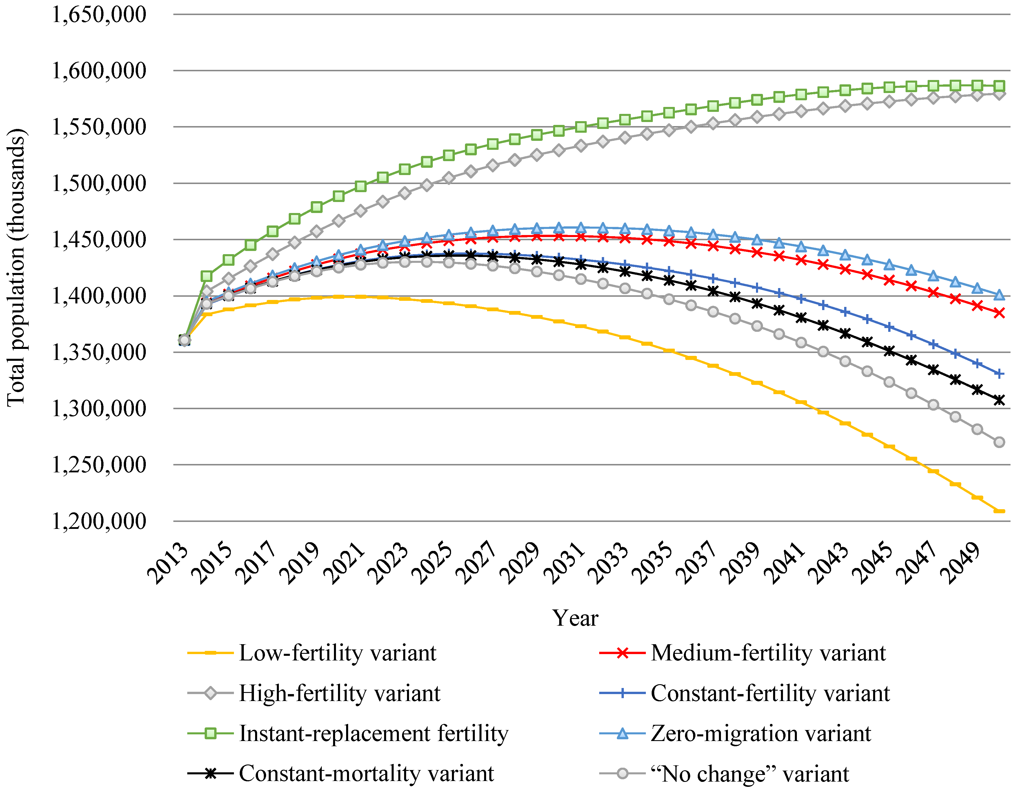
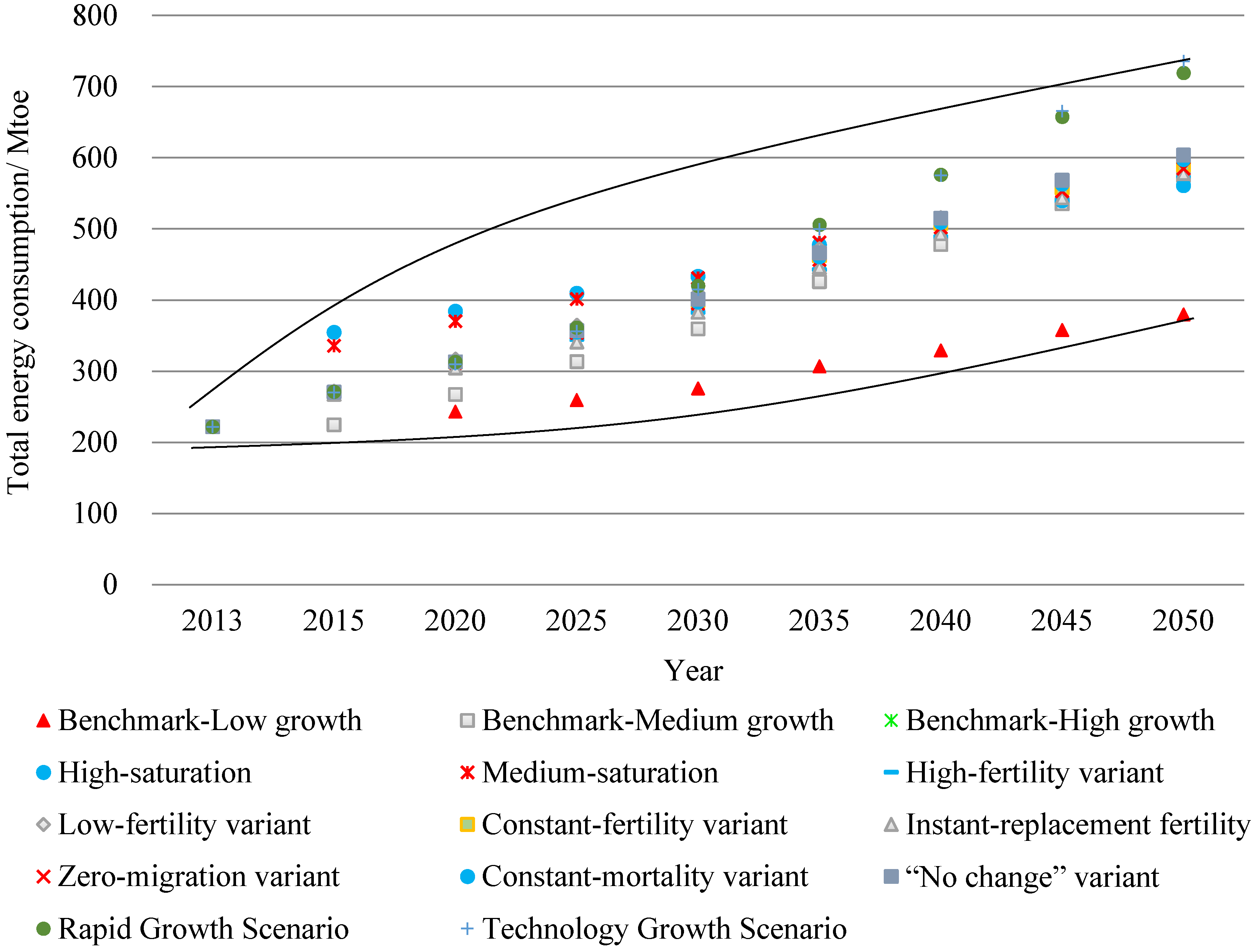
The fourth data set is the 2012 Revision of World Population Prospects (WPP 2012) [52] which is prepared by the United Nations Population Division. WPP 2012 provides a comprehensive and consistent set of annual population data for the world’s countries for 2010–2100, including eight different fertility projection variants based on varying assumptions for fertility, mortality and international migration (low, medium, high, constant-fertility, instant-replacement fertility, constant-mortality variant, zero-migration variant and a “no change” variant). The high, low, constant-fertility and instant-replacement variants differ from the medium variant only in the projected level of total fertility. The constant-mortality variant and the zero-migration variant both employ the same fertility assumption (medium fertility). Lastly, the “no change” variant employs the same assumption of international migration as the medium variant but differs from the latter by having constant fertility and mortality. Among these, we adopt the medium fertility assumption to calculate Chinese GDP per capita. The remaining seven potential fertility trends are used to perform the sensitivity analysis.

The ultimate saturation level of vehicle ownership for each country is obtained from Dargay et al. [20], who estimated vehicle ownership saturation for 45 countries. The on-road fuel economy of the average vehicle and, the share of each major vehicle category to total vehicle population in 2010–2050, are obtained from China Automotive Energy Research Center (CAERC) [44]. CAERC [44] contains estimates of the fuel economy and the share of car, bus and truck to total vehicles in the Business as Usual (BAU) scenario, in which the current trends of vehicle propulsion technologies continue as do existing market conditions and fuel economy improves, but not in an aggressive manner.

3. Results and Discussion

Based on historical information on vehicle growth in OECD countries, the growth patterns in Chinese vehicle stock have been grouped into three scenarios. The first is the high-growth scenario, as witnessed in the North American regions of the United States and Canada. The second is the medium-growth scenario, following the vehicle growth trends witnessed in the Pacific Rim countries including Australia, Japan and New Zealand. The third is the low-growth scenario, following the trends in vehicle growth observed in the following European countries: Austria, Belgium, Denmark, France, Germany, Ireland, Italy, the Netherlands, Norway, Spain, Sweden, Switzerland, and the United Kingdom. The ultimate saturation level of Chinese vehicle ownership is obtained from Dargay et al. [20] and assumes a saturation level of 807 vehicles per 1000 people.

3.1. Results

3.1.1. Curvature Parameters in the Gompertz Function

According to Bollen and Brand [63], fixed-effects (FE) and random-effects (RE) models for longitudinal data are common in sociology because they control for time-invariant omitted variables. Bollen and Brand [63] also point out that the Hausman test is the most typical test used by researchers to compare the performance of these two models.

The results obtained from each regression are shown in Table 2. Columns (1) to (6) present the regression result when Chinese vehicle growth is assumed to follow the North America pattern, Pacific Rim pattern and European pattern, respectively. The first two columns present the results for the high-growth scenario as estimated by RE and FE models. The middle two columns show the medium-growth scenario regression results, and the final two columns present the result for the low-growth scenario.

Table 2. Panel Regression in the Gompertz function.

Dependent Variable: $\text{ln}\left(\text{ln}\frac{V_i^{*}}{V_{i,t}}\right)$
Variable	North America Pattern		Pacific Rim Pattern		European Pattern
	RE	FE	RE	FE	RE	FE
$\frac{E{F}_{i,t}}{\text{10,000}}$	−0.887 ***	−0.755 ***	−0.797 ***	−0.800 ***	−0.436 ***	−0.443 ***
	(−17.60)	(−24.29)	(−28.82)	(−29.29)	(−35.78)	(−36.56)
$\text{ln}\left(-\text{α}\right)$	1.249 ***	0.870 ***	0.960 ***	0.988 ***	0.825 ***	0.844 ***
	(8.30)	(9.41)	(5.10)	(14.82)	(10.66)	(23.12)
N	96	96	139	139	630	630

t statistics has shown in parentheses: *** p < 0.001.

Table 2. Panel Regression in the Gompertz function.

Dependent Variable: $\text{ln}\left(\text{ln}\frac{V_i^{*}}{V_{i,t}}\right)$
Variable	North America Pattern		Pacific Rim Pattern		European Pattern
	RE	FE	RE	FE	RE	FE
$\frac{E{F}_{i,t}}{\text{10,000}}$	−0.887 ***	−0.755 ***	−0.797 ***	−0.800 ***	−0.436 ***	−0.443 ***
	(−17.60)	(−24.29)	(−28.82)	(−29.29)	(−35.78)	(−36.56)
$\text{ln}\left(-\text{α}\right)$	1.249 ***	0.870 ***	0.960 ***	0.988 ***	0.825 ***	0.844 ***
	(8.30)	(9.41)	(5.10)	(14.82)	(10.66)	(23.12)
N	96	96	139	139	630	630

t statistics has shown in parentheses: *** p < 0.001.

Then we apply the Hausman test to establish whether the FE or RE model is the best estimator for projecting growth in the Chinese vehicle market. The null hypothesis states that the RE model is preferable. Table 3 shows that p-value is less than 0.05 for all patterns. These results mean that these two models are different enough to resoundingly reject the null hypothesis for the high-, medium-, and low-growth scenarios so the FE model is our preferred model.

Table 3. The results of the Hausman Test.

Coefficients						Hausman test
	(b) Fixed	(B) Random	(b−B) Difference		Standard Error	chi2 (1)	Prob > chi2
North America pattern
$E{F}_{i,t}$	−0.0000755	−0.0000887	0.0000132	1.67 × 10−6		62.15	0.0000
Pacific Rim pattern
$E{F}_{i,t}$	−0.0000800	−0.0000797	−3.05 × 10−7	1.41 × 10−7		4.68	0.0304
European pattern
$E{F}_{i,t}$	−0.0000443	−0.0000436	−6.37 × 10−7	1.47 × 10−7		18.75	0.0000

Table 3. The results of the Hausman Test.

Coefficients						Hausman test
	(b) Fixed	(B) Random	(b−B) Difference		Standard Error	chi2 (1)	Prob > chi2
North America pattern
$E{F}_{i,t}$	−0.0000755	−0.0000887	0.0000132	1.67 × 10−6		62.15	0.0000
Pacific Rim pattern
$E{F}_{i,t}$	−0.0000800	−0.0000797	−3.05 × 10−7	1.41 × 10−7		4.68	0.0304
European pattern
$E{F}_{i,t}$	−0.0000443	−0.0000436	−6.37 × 10−7	1.47 × 10−7		18.75	0.0000

Table 4 summarizes the curvature parameters α and β from the Gompertz curve. It shows that the absolute value of parameter α in the Asian pattern is larger than that the North American or European pattern, which may lead to greater curvature in the Gompertz function curve when the economic level is low or at zero. The absolute value of parameter β in the Asian pattern is similar to that in North America but larger than that in Europe which may lead to a smoother sloping function curve at high economic levels.

Table 4. The results of curvature parameter estimation.

Parameters	North America Pattern	Pacific Rim Pattern	European Pattern
α	−2.387	−2.686	−2.326
β	−0.755 × 10−4	−0.800 × 10−4	−0.443 × 10−4

Table 4. The results of curvature parameter estimation.

Parameters	North America Pattern	Pacific Rim Pattern	European Pattern
α	−2.387	−2.686	−2.326
β	−0.755 × 10−4	−0.800 × 10−4	−0.443 × 10−4

3.1.2. GDP Growth in China

Based on the results from the CGE model, we estimate the annual GDP growth rate and annual real GDP for the period of from 2014 to 2050 (see Figure 5). Figure 5 shows that the annual GDP growth rate changed at around the year 2020 (see the red dashed line). The rate of growth in annual GDP decreases linearly and slowly from 7.8% in 2013 to 7.1% in 2020. This rate of this decline in annual GDP growth accelerates in the year 2020, reaching a low of 2.3% in 2050. This result suggests that GDP growth in China is set to slow in the post-industrial era at around the year 2020 and therefore the Chinese growth pattern will also change accordingly. However, growth in real GDP increases consistently from 4864 billion dollars in 2013 to 26,745 billion dollars in 2050 (constant 2005 U.S. $, see the black line in Figure 5).

Figure 5. Economic growth trends in China (2013–2050).

Figure 5. Economic growth trends in China (2013–2050).

Based on the estimations of the annual GDP growth rate, we can calculate annual per capita GDP under the medium fertility scenario (see Figure 6). Figure 6 shows that per capita GDP in 2050 is six and half times that in 2013.

Figure 6. Annual Chinese per capita GDP (2013–2050).

Figure 6. Annual Chinese per capita GDP (2013–2050).

3.1.3. Projection of Chinese Vehicle Ownership

We have estimated the curvature parameters of the Gompertz function in Section 3.1.1 based on high-, medium-, and low-growth scenarios, as represented by vehicle development trends in North America, the Pacific Rim and Europe respectively. A CGE model was used to estimate annual per capita GDP in China for the years 2013–2050. We assumed a Chinese saturation level of 807 vehicles per 1000 people in Section 2.4 and project Chinese vehicle ownerships according to Equation (1) (see Figure 7).

Figure 7. Projected Chinese vehicle ownership (2013–2050). Vehicle ownership data for China in 2013 is obtained from the National Bureau of Statistics 2013.

Figure 7. Projected Chinese vehicle ownership (2013–2050). Vehicle ownership data for China in 2013 is obtained from the National Bureau of Statistics 2013.

Since annual per capita GDP increases monotonically in China over the coming decades, Figure 7 also depicts the Gompertz curve. The results show that vehicle ownership increases along with per capita GDP, which means that growth in Chinese vehicle ownerships has not reached the saturated level (the growth rate of Gompertz S-curve is decreasing) in 2050 for either scenario. Vehicle stocks in the medium-growth scenario may approximate those in the high-growth scenario in the year 2050 due to the large absolute value of curvature parameters α and β. For the high-growth scenario, there is a small jump between 2013 and 2014 before the growth pattern in Chinese vehicle ownership enters the high growth path. Due to the small absolute value of curvature parameters β, growth in Chinese vehicle ownership may be unable to match the robust growth rates observed in European countries.

Furthermore, we need to ensure whether growth in Chinese vehicle ownerships remains in the incubation period (characterized by an initial slow growth) or, alternatively, whether Chinese vehicle growth has entered the booming period (characterized by rapid growth). Unlike the incubation period, the booming period includes the inflection point.

Figure 8 shows that the increasing curve reaches the inflection point at around the year 2020 in each growth scenario. It means that growth in Chinese vehicle ownerships has been in transition throughout the second half of the booming period (and therefore, over the inflection point) since 2020. Furthermore, the growth rate in vehicle ownerships is highest in the medium-growth scenario, due to the large absolute value of curvature parameters α and β.

Figure 8. Growth in Chinese vehicle demand under different economic growth patterns.

Figure 8. Growth in Chinese vehicle demand under different economic growth patterns.

3.1.4. The Energy Demand of Road Vehicles

Having derived the annual vehicle population of China, we can use Equation (7) to estimate the total energy consumption of road vehicles—including cars, buses and trucks—under each growth scenario. Table 5 summarizes the results for 2013 and for every consecutive 5 year period from 2015 to 2040.

Our model estimates that the total energy consumption of road vehicles in 2050 is 380, 575 and 586 million tonnes of oil equivalent (Mtoe) for low-, medium-, and high-growth scenarios, respectively. These results are consistent with those obtained in Ou et al. [54], a study which estimated that, by 2050, the direct energy demand in China’s road transport sector will be 564 Mtoe in the BAU case. When energy consumption is disaggregated by mode of road-transport vehicle, it is apparent that cars and trucks have accounted for over 90% of the total energy consumption of road vehicles in China since 2015. This result is consistent with Wu’s [25] projections of the fuel consumption shares of different road vehicles for the year 2030. Wu [25] estimated that the fuel consumption share of heavy-duty trucks (HDT), other trucks, buses and cars are 39%, 14%, 12% and 35%, respectively.

Table 5. Energy consumption of road vehicles in China (Unit: Mtoe).

Year	Low-Growth Scenario				Medium-Growth Scenario				High-Growth Scenario
	Car	Bus	Truck	Total	Car	Bus	Truck	Total	Car	Bus	Truck	Total
2013	101.6	22.6	93.1	217.4	101.6	22.6	93.1	217.4	101.6	22.6	93.1	217.4
2015	115.0	20.5	89.4	225.0	114.8	20.5	89.2	224.5	138.2	24.7	107.4	270.3
2020	130.8	19.2	93.2	243.2	143.7	21.1	102.5	267.3	167.6	24.6	119.5	311.7
2025	132.1	19.5	107.7	259.3	159.5	23.6	130.1	313.2	180.0	26.6	146.9	353.5
2030	137.5	19.8	118.3	275.6	179.4	25.8	154.3	359.5	196.8	28.3	169.4	394.5
2035	147.1	21.6	138.0	306.7	204.2	29.9	191.7	425.8	218.6	32.1	205.2	455.8
2040	155.1	23.0	151.0	329.0	225.2	33.4	219.3	477.9	236.2	35.0	230.0	501.2
2045	166.7	25.4	165.6	357.7	249.4	38.0	247.8	535.1	257.0	39.1	255.4	551.6
2050	176.8	27.4	175.5	379.7	267.9	41.5	266.0	575.4	272.7	42.2	270.7	585.5

Table 5. Energy consumption of road vehicles in China (Unit: Mtoe).

Year	Low-Growth Scenario				Medium-Growth Scenario				High-Growth Scenario
	Car	Bus	Truck	Total	Car	Bus	Truck	Total	Car	Bus	Truck	Total
2013	101.6	22.6	93.1	217.4	101.6	22.6	93.1	217.4	101.6	22.6	93.1	217.4
2015	115.0	20.5	89.4	225.0	114.8	20.5	89.2	224.5	138.2	24.7	107.4	270.3
2020	130.8	19.2	93.2	243.2	143.7	21.1	102.5	267.3	167.6	24.6	119.5	311.7
2025	132.1	19.5	107.7	259.3	159.5	23.6	130.1	313.2	180.0	26.6	146.9	353.5
2030	137.5	19.8	118.3	275.6	179.4	25.8	154.3	359.5	196.8	28.3	169.4	394.5
2035	147.1	21.6	138.0	306.7	204.2	29.9	191.7	425.8	218.6	32.1	205.2	455.8
2040	155.1	23.0	151.0	329.0	225.2	33.4	219.3	477.9	236.2	35.0	230.0	501.2
2045	166.7	25.4	165.6	357.7	249.4	38.0	247.8	535.1	257.0	39.1	255.4	551.6
2050	176.8	27.4	175.5	379.7	267.9	41.5	266.0	575.4	272.7	42.2	270.7	585.5

3.2. Discussion on Key Factors

Figure 9 compares the vehicle stock projections estimated in this paper with those obtained by other studies. Figure 9 shows that vehicle stock projections based on the low-growth scenario in this study are lower than the projections contained in the majority of studies from the last two decades. During the period under the study, the vehicle stock projections based on the medium-, and high-growth scenarios in this study are also similar to those obtained under assumptions of high-growth in Huo et al. [24], but lower than that in Wu et al. [15]. The projected results obtained in this study are lower than those obtained by Wang et al. [27] across all three growth scenarios.

There are two main explanations for these differences. Firstly, this study employs a different method of estimating the long-term GDP growth rate and the GDP growth rate used will influence estimations of absolute vehicle ownership levels. Secondly, this study adopts different parameter settings—on vehicle saturation levels, for instance—and the parameter settings influence the shape of the Gompertz curve, which is driven by the curvature parameters α and β. In the following sections, we estimate vehicle ownership levels under varying vehicle saturation levels, GDP growth rates and population growth rates.

Figure 9. Vehicle stock projections across various studies.

Figure 9. Vehicle stock projections across various studies.

3.2.1. Sensitivity Analysis of Vehicle Saturation Levels

Using data from several sources [15,19,20], the first sensitivity analysis illustrates the effect on vehicle ownership projections of varying vehicle saturation levels. Table 6 presents the ultimate vehicle ownership saturation level and the two curvature parameters in the Gompertz function based on the vehicle consumption patterns from North America; the saturation level of vehicle ownership is highest in Dargay and Gately [19], followed by Wu et al. [15] and Dargay et al. [20]. Therefore, we refer to these three scenarios as high-, medium-, and low-saturation scenarios, respectively.

The default saturation level of China’s vehicle stock is 807 vehicles per 1000 people. When all other variables are held at their base values, the absolute value of the two curvature parameters α and β decrease with increasing vehicle saturation levels (see the last two rows in Table 6).

Table 6. Varying vehicle saturation levels and curvature parameters in the Gompertz function.

Country	Low-Saturation	Medium-Saturation	High-Saturation
	Dargay et al. [20]	Wu et al. [15]	Dargay and Gately [19]
Canada	845	860	910
United States	852	875	890
α	−2.387	−2.010	−1.896
β	−0.755 × 10−4	−0.654 × 10−4	−0.597 × 10−4

Table 6. Varying vehicle saturation levels and curvature parameters in the Gompertz function.

Country	Low-Saturation	Medium-Saturation	High-Saturation
	Dargay et al. [20]	Wu et al. [15]	Dargay and Gately [19]
Canada	845	860	910
United States	852	875	890
α	−2.387	−2.010	−1.896
β	−0.755 × 10−4	−0.654 × 10−4	−0.597 × 10−4

Figure 10 illustrates the impact of different vehicle saturation levels on Chinese vehicle stock projections. The Gompertz curve steepens as vehicle saturation levels decrease; in other words, the Gompertz curve becomes steeper because of increases in the absolute value of the two curvature parameters α and β.

However, vehicle saturation levels have no influence on the inflection point of the Gompertz curve (see Figure 11).

Figure 10. Sensitivity analysis of vehicle saturation level on vehicle ownership: vehicle stocks.

Figure 10. Sensitivity analysis of vehicle saturation level on vehicle ownership: vehicle stocks.

Figure 11. Sensitivity analysis of vehicle saturation level on vehicle ownership: Growth rate.

Figure 11. Sensitivity analysis of vehicle saturation level on vehicle ownership: Growth rate.

In sum, the values of the two curvature parameters α and β solely influence the slope of the Gompertz curve whereas growth in vehicle demand is determined by the economic indicator, as will be demonstrated in Section 3.2.2.

3.2.2. Sensitivity Analysis of GDP Growth

There is considerable uncertainty over China’s future economic development. Therefore, the second sensitivity analysis investigates the effects of different GDP growth rates on vehicle ownership projections. We forecast China’s future economic growth rate under three scenarios.

The baseline scenario is based on our own setting, a relatively mild growth path. The other two scenarios are based on the benchmark scenario outlined in Li [41]. We use Li’s [41] 5-year average growth rate estimates to generate two growth paths—a rapid growth scenario and a technology growth scenario. In the rapid growth scenario, the economic growth rate declines annually and total productivity growth declines at a relatively constant rate. In the technology growth scenario, the rate of economic growth increases slightly in the last decade of the study period, mostly because of mild increases in total factor productivity.

The growth in total factor productivity (mainly technology) will have a significant influence on the development of China’s automobile industry. Therefore, these sensitivity analyses enable us to test the robustness of our vehicle ownership projections to varying growth paths. This is important because China’s future economic development is uncertain, as previously mentioned. The impact of different GDP growth rates on Chinese economic development are illustrated in Figure 12.

Figure 12. Projected economic growth under different economic growth scenarios.

Figure 12. Projected economic growth under different economic growth scenarios.

Using Equation (1), we estimate Chinese vehicle ownership under three different projections of Chinese economic growth. The remaining default parameters are set at the level observed in North America, specifically α = −2.387, β = −0.755 × 10⁻⁴ and V_China* = 807. Figure 13 demonstrates that economic growth can promote the development of the automotive industry; the smooth upwards slope in vehicle ownership is driven by the steep, upwards slope in GDP growth. Conversely, this result indicates that a rapid decline in economic growth could lead to a decline in the rate of vehicle consumption.

Figure 13. Sensitivity analysis under different GDP growth paths: vehicle stocks.

Figure 13. Sensitivity analysis under different GDP growth paths: vehicle stocks.

Regardless of the rate at which China’s economy grows, our results indicate that growth in Chinese vehicle demand will be determined by the economic indicator, as noted in Section 3.2.1. The importance of the relationship between GDP and vehicle demand is further illustrated in Figure 14.

Figure 14. Sensitivity analysis under different GDP growth paths: growth rate.

Figure 14. Sensitivity analysis under different GDP growth paths: growth rate.

The following insights can be derived from Figure 14. Firstly, the inflection point of the Gompertz curve is lagged under rapid economic development; this implies that policymakers could use economic policy to indirectly stimulate vehicle demand (see the vertical lines in Figure 14). Secondly, with continued future economic and technological advancement, the growth rate of vehicle stocks may be non-monotonic in the booming period. However, such exogenous shocks only take effect in the short-term; until around the year 2040 (see the dashed area that represents the technology growth scenario and compare it to the other two scenarios in Figure 14).

3.2.3. Sensitivity Analysis of Population Growth

Population growth indirectly affects vehicle ownerships owing to its joint determination of GDP per capita and the GDP growth rate. As discussed in the Section 2.4, the WPP 2012 [52] provides different population projections for China based on eight fertility projection variants. The variation in the estimated projections of Chinese fertility are obtained by varying the assumed values for fertility, mortality and international migration (low, medium, high, constant-fertility, instant-replacement fertility, constant-mortality variant, zero-migration variant and “no change” variant). In this section, the influence of population growth on vehicle demand is calculated using all eight Chinese fertility scenarios.

Figure 15 summarizes the data on annual total population for China. With the exception of the high-fertility and instant-replacement fertility scenarios, the estimates of Chinese population growth under the varying fertility scenarios are remarkably similar; Chinese population growth is consistently expected to increase until around the year 2025 to 2030 but to decrease thereafter. Conversely, under high-fertility and instant-replacement fertility scenarios, Chinese population growths are expected to increase rapidly well before becoming stable in the last decade of the period under study.

Figure 15. Annual population of China under varying fertility trends (data source: [52]).

Figure 15. Annual population of China under varying fertility trends (data source: [52]).

In this section, we vary the method by which Chinese population growth is estimated to illustrate the impact of demographic indicators on Chinese vehicle stock projections (Figure 16). The base case assumes that Chinese fertility levels will follow the medium fertility scenario. The other default parameter set according to the vehicle development rends witnessed in North America, namely α = −2.387, β = −0.755 × 10⁻⁴ and V_China* = 807.

Figure 16. Sensitivity analyses under varying Chinese population growth rates.

Figure 16. Sensitivity analyses under varying Chinese population growth rates.

Estimated Chinese vehicle demand under different population growth scenarios yields results very similar to those in Wu et al. [15], suggesting that demographic variables have a very weak impact on vehicle stock projections. This indicates that the first driving force is economic factors rather than demographic developments, especially when the demographic structure is relatively stable.

3.2.4. Energy Consumption Projections under Different Scenarios

We have discussed the impact of varying economic growth rates, vehicle saturation levels and fertility on projected vehicle ownership, including three baseline growth scenarios, two additional saturation cases, two additional GDP growth paths and eight fertility variants. Using Equation (7), we calculate the aggregate energy consumption of each of the major vehicle categories (cars, buses and trucks) for each five year period from 2013 to 2050. The dashed area represents the degree of influence exercised by each explanatory factor on energy consumption projections for road transport (see Figure 17).

As the “Energy consumption projection” band illustrates, energy consumption by road vehicles is lowest under the baseline low-growth scenario with medium fertility. Our results estimate that energy demand will be highest under two scenarios: (1) the high-growth scenario with high vehicle saturation levels in the first decade and (2) the high-growth scenario with higher GDP growth rates and technological advancement in the last decade. The following insights can be obtained from Figure 17.

(1). The band of potential energy demand shows a variation of about 300 Mtoe in 2020 and about 350 Mtoe in 2050, which indicate that Chinese government needs to make essential policy to safeguard the substantial amount of energy, especially for the accumulated amount from 2013 to 2050.

(2). The increasing certain amount of GHG emissions depending on the energy sources used associated with substantial amount of energy use may bring a great challenge to China and even the whole world.

(3). In the future, Chinese government needs to establish the fuel economy standards much more strict to provide a vehicle development scheme towards low-carbon or energy efficient transportation.

Figure 17. Total energy consumption of road vehicles under different scenarios.

Figure 17. Total energy consumption of road vehicles under different scenarios.

4. Concluding Remarks

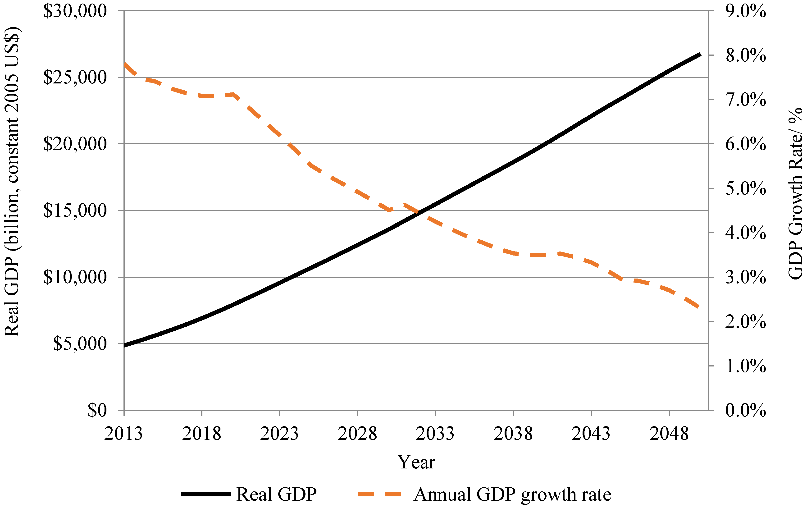
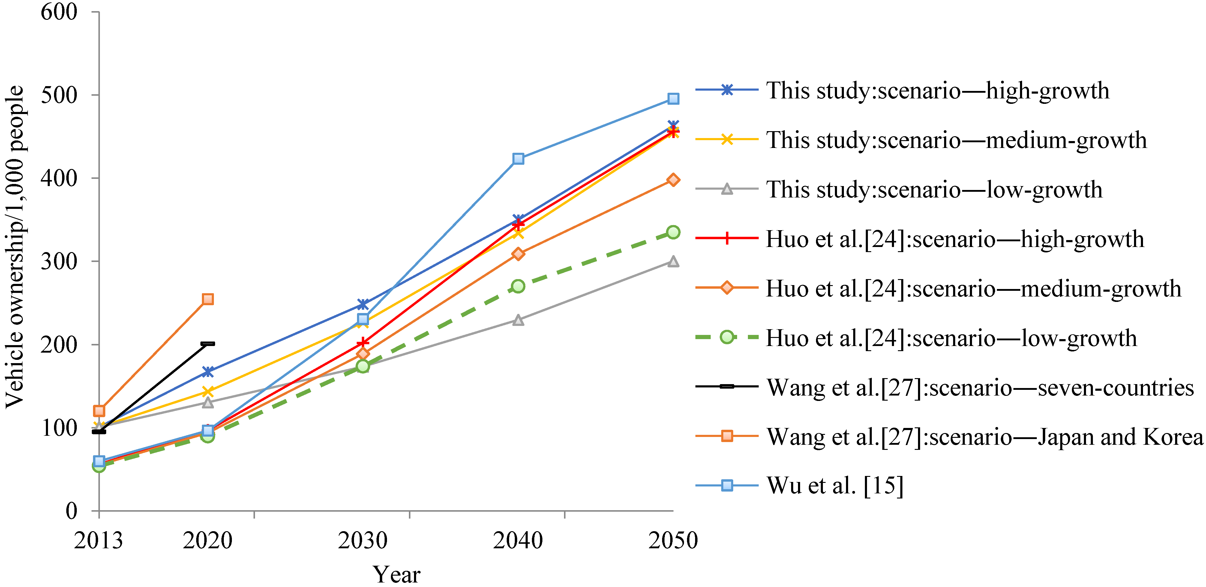
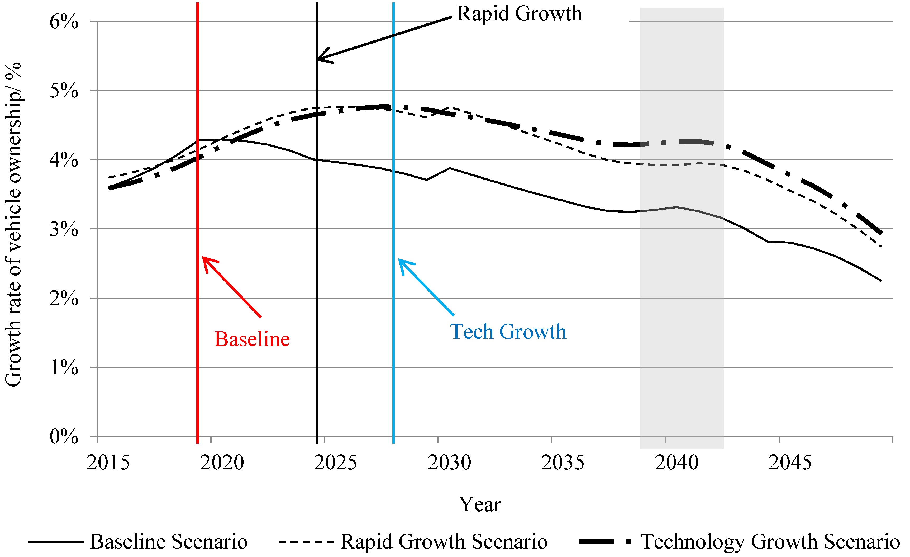
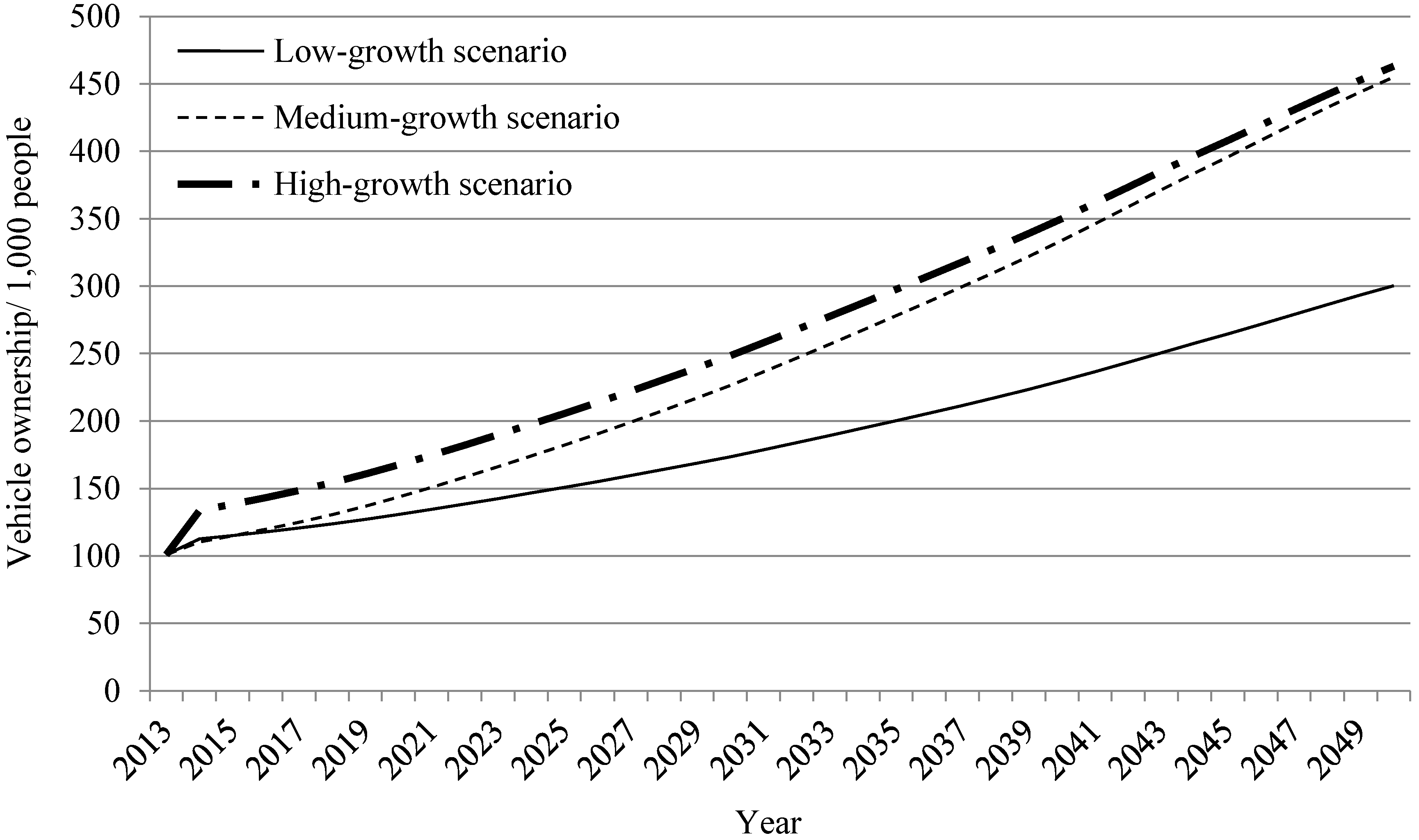
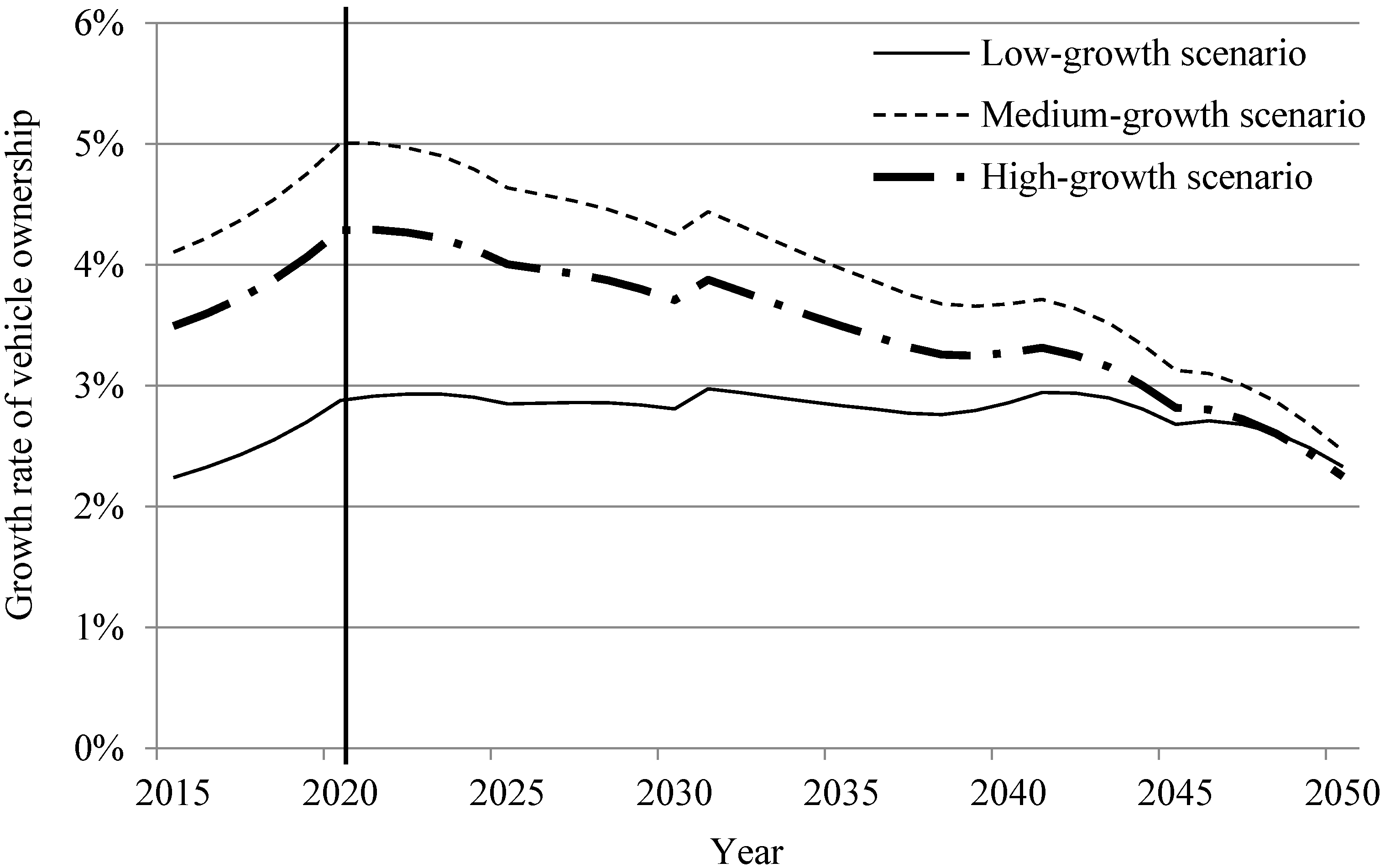
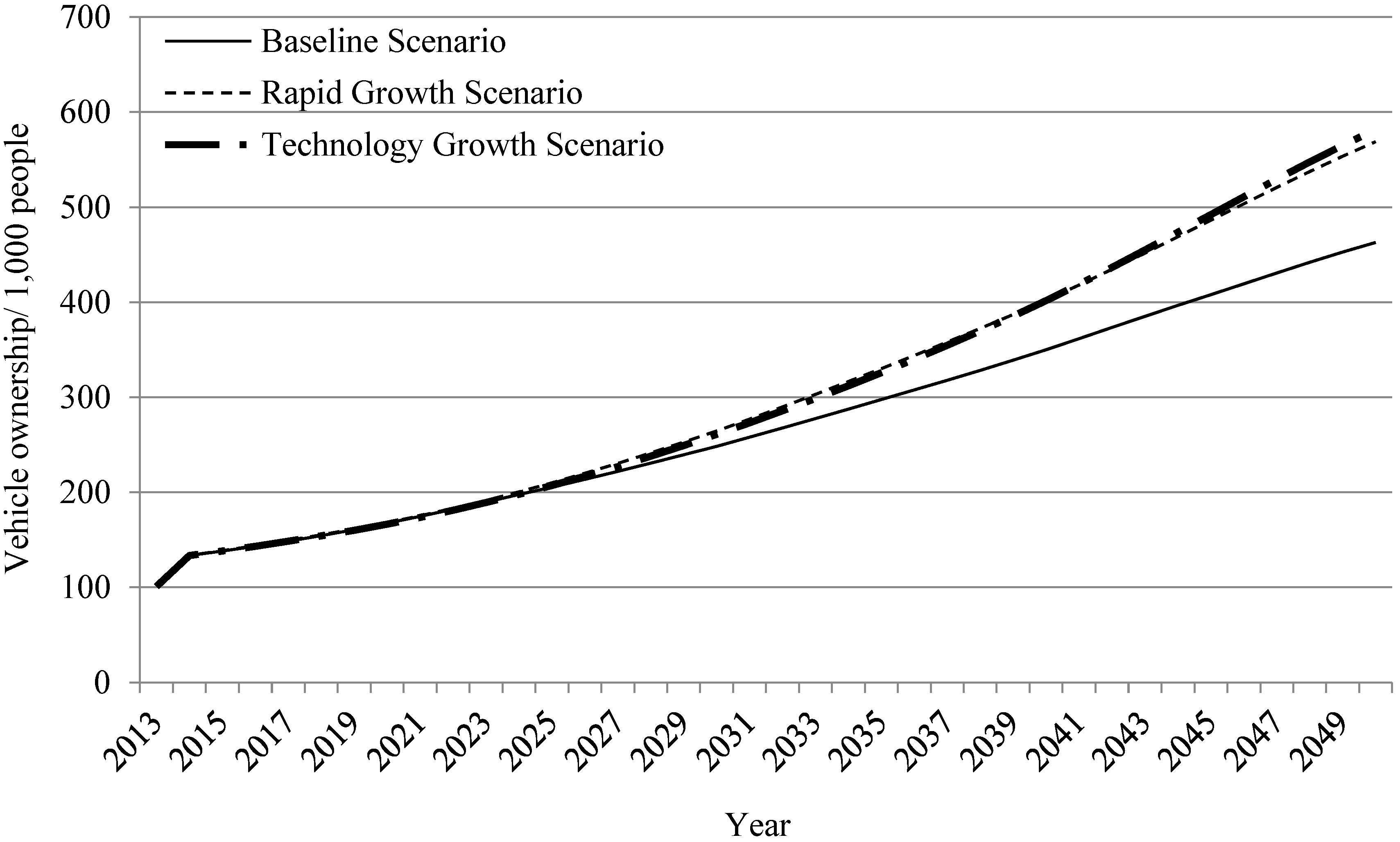
This study projects that, by 2050, vehicle ownership in China will reach 300, 455 and 463 vehicles per 1000 people under low-, medium-, and high-growth scenarios, respectively. Our results suggest that China’s vehicle stock will be of a similar size regardless of whether the Chinese economy grows at a high or medium rate. Growth in Chinese vehicle ownership will not reach the saturation point by the year 2050 under either the medium or high growth scenarios. However, vehicle demand will enter the booming period during the period from now to 2050 and is estimated to reach the inflection point of the Gompertz curve at around the year 2020.

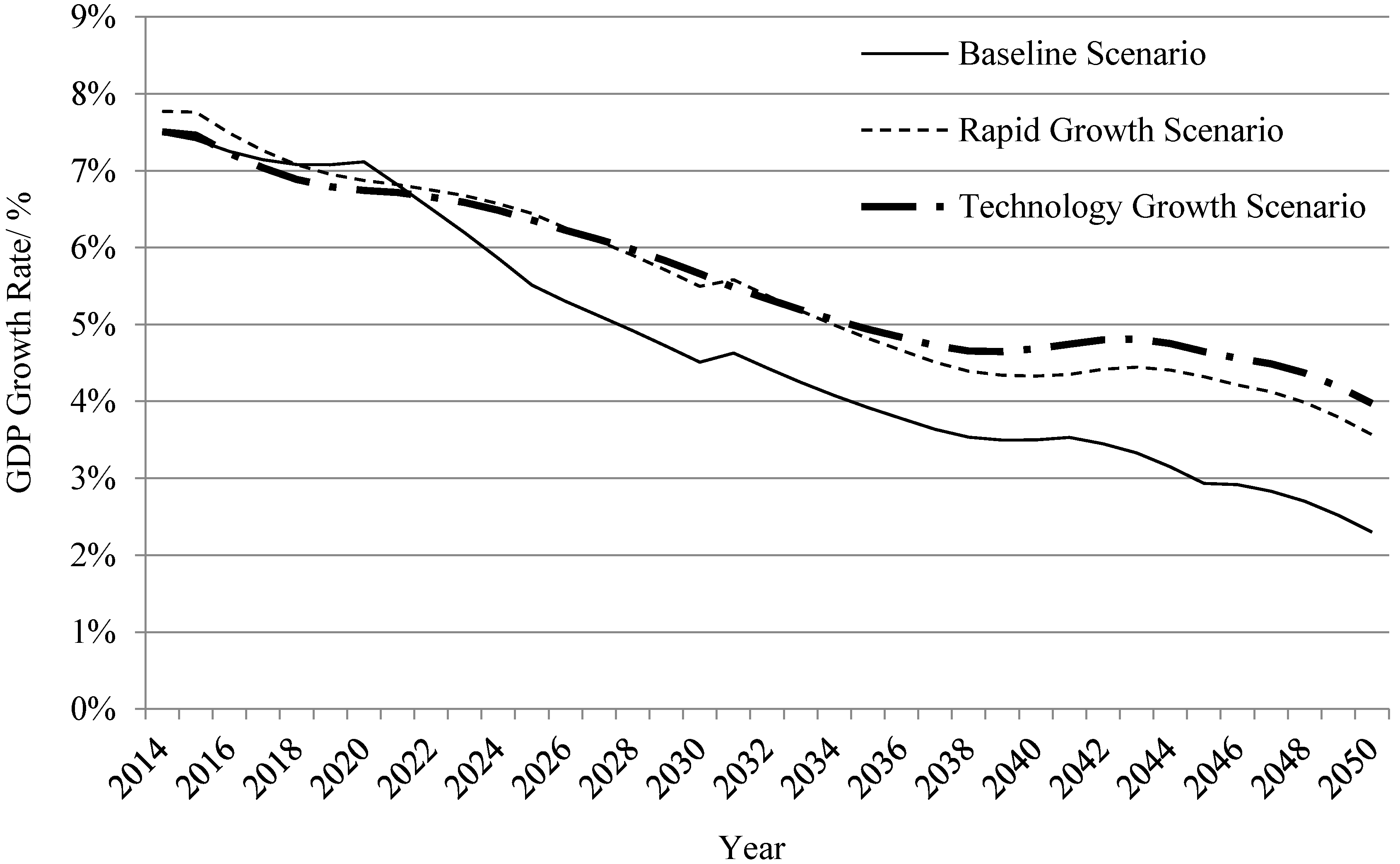
According to our forecasts, Chinese economic growth declines steadily until the year 2030. After 2030, our model approximates the steady state due to the exogenous population growth and total factor productivity plays a significant role in determining the economic growth rate during the period 2030–2050. The trade-off between growth in total factor productivity and growth in the Chinese labor force decreases after 2030, giving rise to different economic growth paths under different scenarios.

Our results suggest that the total energy consumption of road vehicles will reach 380, 580 and 590 Mtoe in 2050 under low-, medium-, and high-growth scenarios, respectively. Moreover, our results estimate that more than 90% of the road transport industry’s total fuel consumption will be consumed by cars and trucks by the year 2015. Finally, our results suggest that energy demand in the road transport industry will be highest under the high vehicle saturation with high-growth scenario and lowest under the baseline low-growth scenario.

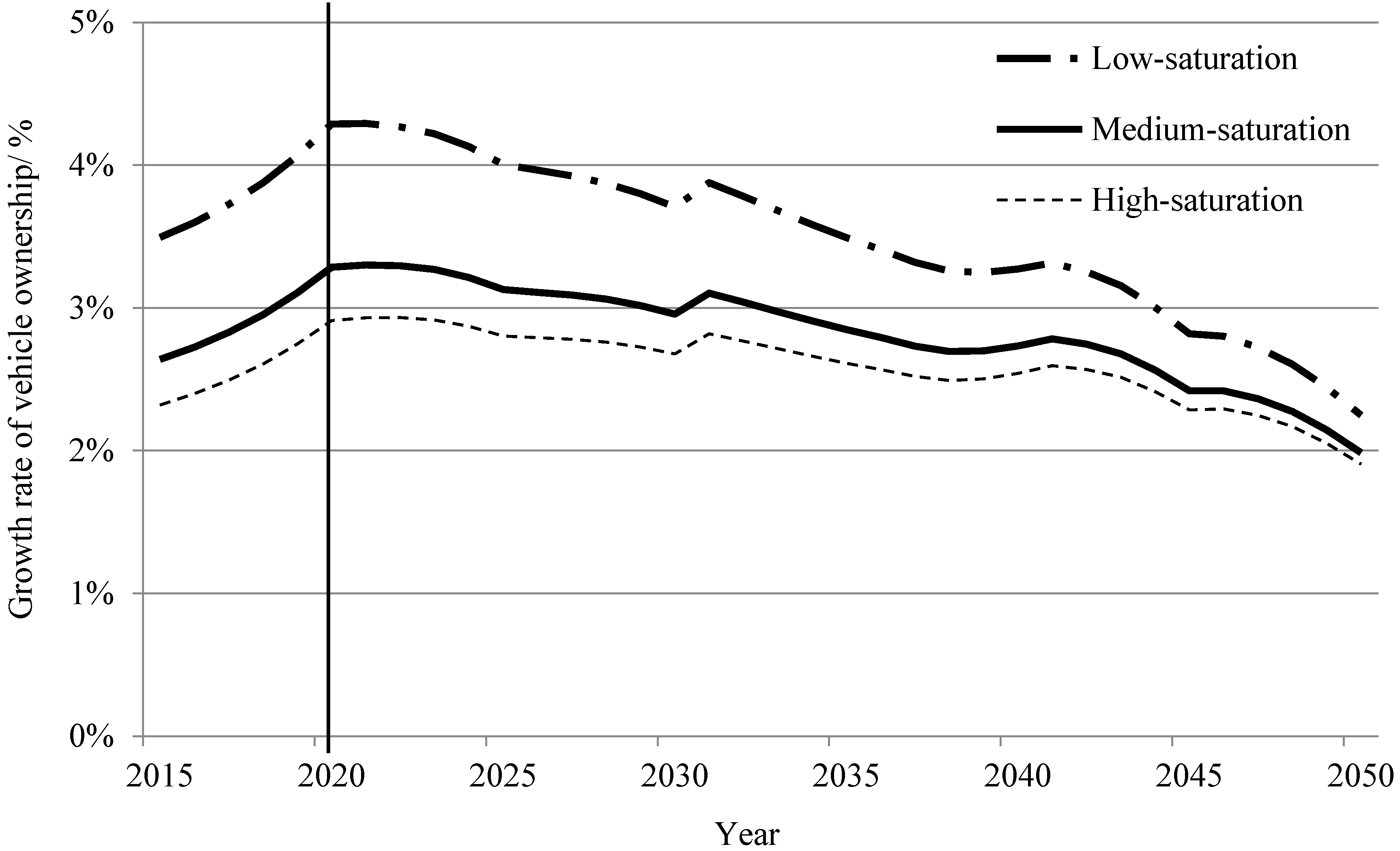
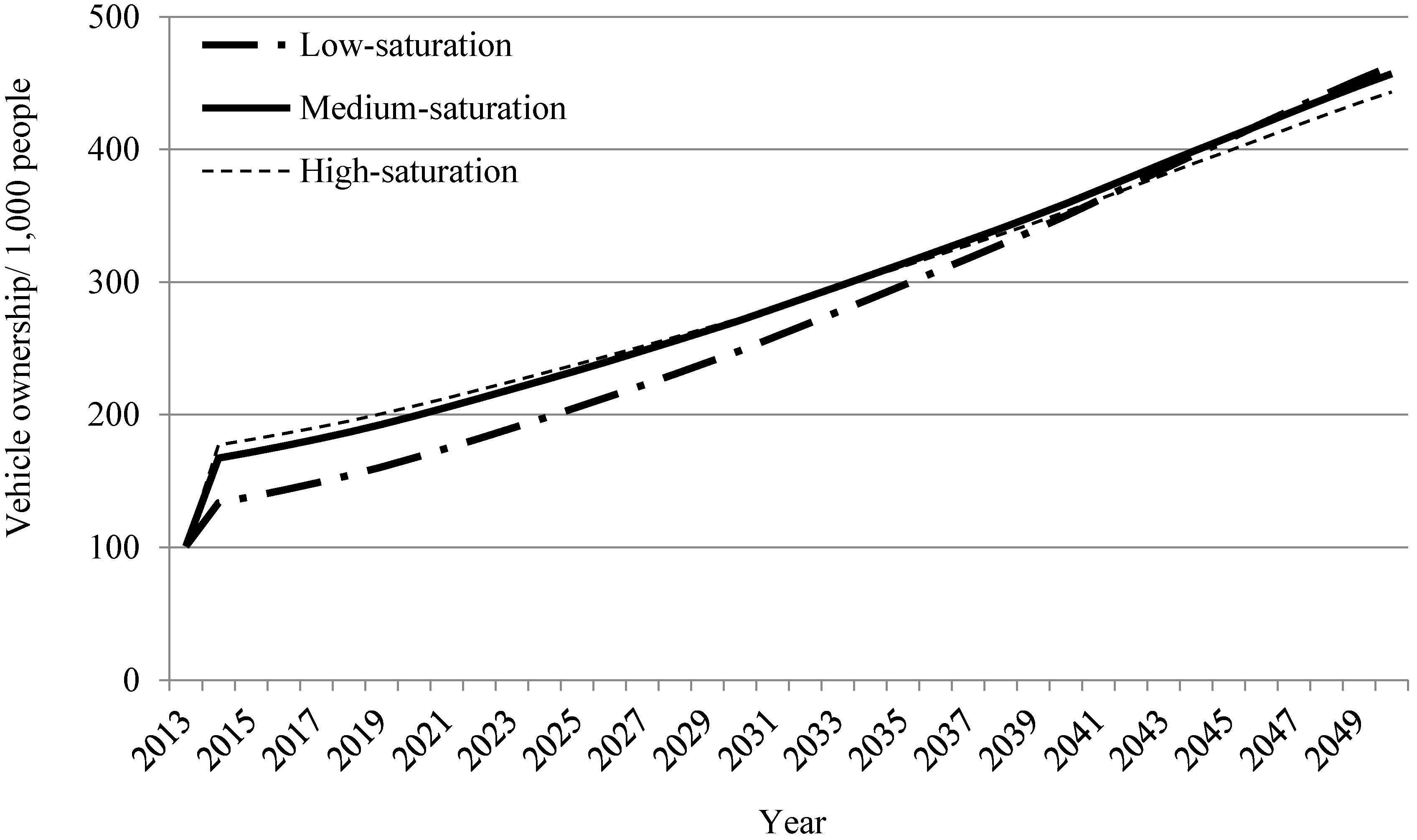
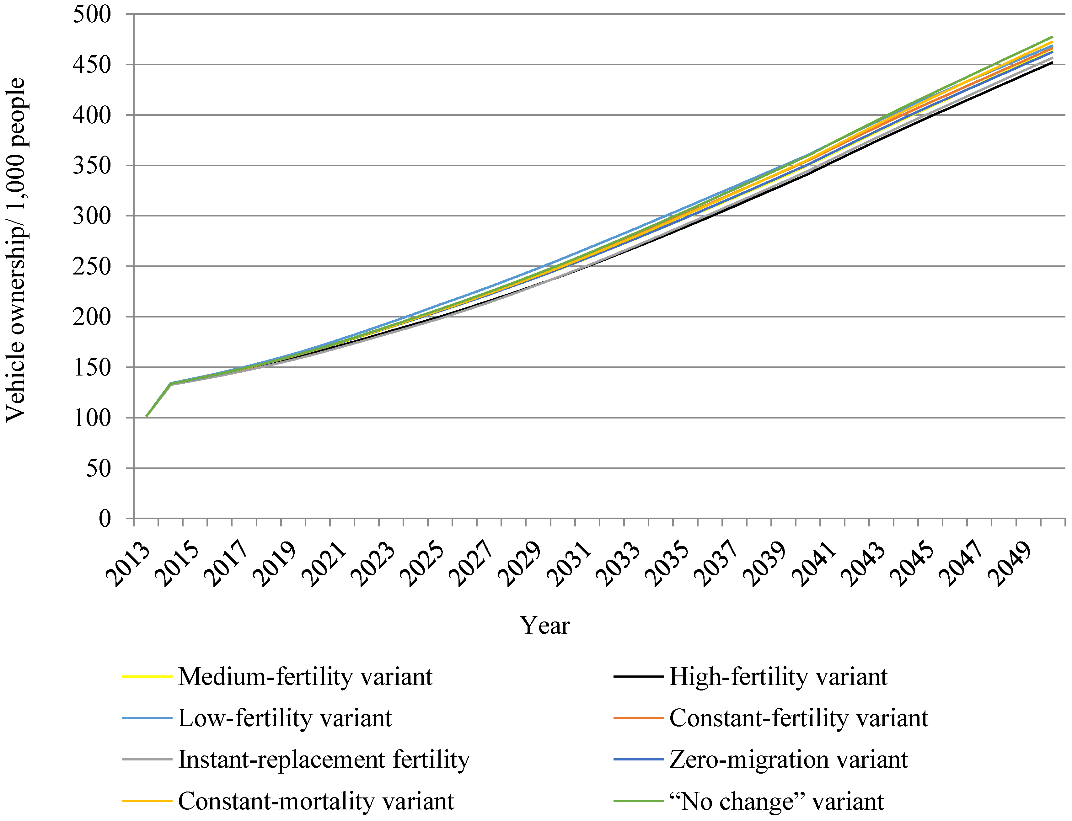
The sensitivity analyses results suggest that: vehicle saturation levels only influence the shape of the growth in Chinese vehicle stocks; population growth has a weak impact on vehicle demand and; the economic indicator, GDP per capita, is the dominant factor explaining growth in Chinese vehicle demand. Furthermore, with the exception of population growth estimates, vehicle ownership projections are sensitive to all of the key explanatory factors (economic growth and the vehicle saturation level). The projection of Chinese vehicle demand could be influenced by different variables such as for instance public policies, government intervention, and the variation between different regions. An important implication of this result is that, to further improve the accuracy of Chinese vehicle demand, in-depth scenario analysis on different influencing factors are necessary.

There are several important policy implications for energy demand, greenhouse gas emissions and traffic congestion in China. The likely growth in China’s vehicle stock suggests that China’s automotive industry will become a huge consumer of energy. Policymakers should therefore consider increasing vehicle energy efficiency standards, changing consumer energy consumption patterns and reducing the transportation sector’s high dependency on fossil fuels. Several energy consumption policies should be introduced across China to reduce the energy demand of on-road vehicles, such as the car License Auction Policy in Shanghai [64] and Beijing’s Vehicle Lottery [65]. These government interventions and regulations could help to restrict vehicle demand and therefore energy consumption by the transport industry. The boom in China’s automotive industry poses a great challenge to the environment, especially in relation to greenhouse gas emissions. It is therefore essential to promote the use of low-emission vehicles such as hybrid electric vehicles, electric vehicles and fuel cell vehicles. Policymakers should also increase exhaust emission standards and introduce regulations for all vehicle engines, including conventional internal combustion engines. Developed Chinese cities—including some provincial capitals, industrial and coastal cities—have the highest numbers of road vehicles [26]. Chronic traffic jams could be reduced by promoting the use of public transport in these cities. Alternatively, the government may wish to consider reducing the imbalance in Chinese regional development and population density in developed cities.

References

1. Waraich, R.A.; Galus, M.D.; Dobler, C.; Balmer, M.; Andersson, G.; Axhausen, K.W. Plug-in hybrid electric vehicles and smart grids: Investigations based on a microsimulation. Transp. Res. Part C Emerg. Technol. 2013, 28, 74–86. [Google Scholar] [CrossRef]
2. Yuan, J.H.; Hou, Y.; Xu, M. China’s 2020 carbon intensity target: Consistency, implementations, and policy implications. Renew. Sustain. Energy Rev. 2012, 16, 4970–4981. [Google Scholar] [CrossRef]
3. Ou, X.; Yan, X.; Zhang, X.; Zhang, X. Life-Cycle Energy Use and Greenhouse Gas Emissions Analysis for Bio-Liquid Jet Fuel from Open Pond-Based Micro-Algae under China Conditions. Energies 2013, 6, 4897–4923. [Google Scholar] [CrossRef] [Green Version]
4. Organisation for Economic Co-operation and Development (OECD)/International Energy Agency (IEA). World Energy Outlook 2013; OECD/IEA: London, UK, 2013. [Google Scholar]
5. Wang, G.; Bai, S.; Ogden, J.M. Identifying contributions of on-road motor vehicles to urban air pollution using travel demand model data. Transp. Res. Part D Transp. Environ. 2009, 14, 168–179. [Google Scholar] [CrossRef]
6. Balat, M.; Balat, H. Recent trends in global production and utilization of bio-ethanol fuel. Appl. Energy 2009, 86, 2273–2282. [Google Scholar] [CrossRef]
7. Zhang, K.; Batterman, S. Air pollution and health risks due to vehicle traffic. Sci. Total Environ. 2013, 450, 307–316. [Google Scholar] [CrossRef] [PubMed]
8. International Maritime Organization (IMO). Second IMO GHG Study 2009; IMO: London, UK, 2009. [Google Scholar]
9. Gao, L.; Winfield, Z.C. Life Cycle Assessment of Environmental and Economic Impacts of Advanced Vehicles. Energies 2012, 5, 605–620. [Google Scholar] [CrossRef]
10. Hao, H.; Wang, H.; Ouyang, M. Comparison of policies on vehicle ownership and use between Beijing and Shanghai and their impacts on fuel consumption by passenger vehicles. Energy Policy 2011, 39, 1016–1021. [Google Scholar] [CrossRef]
11. Li, J.; Zuylen, H.J. Road Traffic in China. Procedia-Soc. Behav. Sci. 2014, 111, 107–116. [Google Scholar] [CrossRef]
12. TomTom Traffic Index. 2014. Available online: http://www.tomtom.com/en_gb/trafficindex (accessed on 15 August 2014).
13. Hatani, F. The logic of spillover interception: The impact of global supply chains in China. J. World Bus. 2009, 44, 158–166. [Google Scholar] [CrossRef]
14. Huo, H.; Zhang, Q.; He, K.; Yao, Z.; Wang, X.; Zheng, B.; Streets, D.G.; Wang, Q.; Ding, Y. Modelling vehicle emissions in different types of Chinese cities: Importance of vehicle fleet and local features. Environ. Pollut. 2011, 159, 2954–2960. [Google Scholar] [CrossRef] [PubMed]
15. Wu, T.; Zhao, H.; Ou, X. Vehicle Ownership Analysis Based on GDP per Capita in China: 1963–2050. Sustainability 2014, 6, 4877–4899. [Google Scholar] [CrossRef]
16. Huo, H.; Wang, M.; Zhang, X.; He, K.; Gong, H.; Jiang, K.; Jin, Y.; Shi, Y.; Yu, X. Projection of energy use and greenhouse gas emissions by motor vehicles in China: Policy options and impacts. Energy Policy 2012, 43, 37–48. [Google Scholar] [CrossRef]
17. Huo, H.; Wang, M. Modeling future vehicle sales and stock in China. Energy Policy 2012, 43, 17–29. [Google Scholar] [CrossRef]
18. Dargay, J.M.; Gately, D. Income’s effect on car and vehicle ownership, worldwide: 1960–2015. Transp. Res. Part A Policy Pract. 1999, 33, 101–138. [Google Scholar] [CrossRef]
19. Dargay, J.M.; Gately, D. Modelling Global Vehicle Ownership. In Proceedings of the WCTR Conference, Seoul, Korean, 1 July 2001.
20. Dargay, J.M.; Gately, D.; Sommer, M. Vehicle ownership and income growth, worldwide: 1960–2030. Energy J. 2007, 28, 143–170. [Google Scholar] [CrossRef]
21. Meyer, I.; Leimbach, M. Global car demand and climate change: A regionalized analysis into growth patterns of vehicle fleets, CO2 emissions, and abatement strategies. In Proceedings of the Transport—The Next 50 Years Conference, Christchurch, New Zealand, 25–27 July 2007.
22. Keshavarzian, M.; Kamali Anaraki, S.; Zamani, M.; Erfanifard, A. Projections of oil demand in road transportation sector on the basis of vehicle ownership projections, worldwide: 1972–2020. Econ. Model. 2012, 29, 1979–1985. [Google Scholar] [CrossRef]
23. Meyer, I.; Kaniovski, S.; Scheffran, J. Scenarios for regional passenger car fleets and their CO2 emissions. Energy Policy 2012, 41, 66–74. [Google Scholar] [CrossRef]
24. Huo, H.; Wang, M.; Johnson, L.; He, D. Projection of Chinese motor vehicle growth, oil demand, and CO2 Emissions through 2050. Transp. Res. Rec. J. Transp. Res. Board 2007, 2038, 69–77. [Google Scholar] [CrossRef]
25. Wu, Y. Projection of Chinese Motor Vehicle Growth CO2 and Emissions through 2030 with Different Propulsion/Fuel System Scenarios. In Proceedings of the JARI China Round Table, Beijing, China, 19 October 2009.
26. Zheng, B.; Huo, H.; Zhang, Q.; Yao, Z.L.; Wang, X.T.; Yang, X.F.; Liu, H.; He, K.B. A new vehicle emission inventory for China with high spatial and temporal resolution. Atmos. Chem. Phys. Discuss. 2013, 13, 32005–32052. [Google Scholar] [CrossRef]
27. Wang, Y.; Teter, J.; Sperling, D. China’s soaring vehicle population: Even greater than forecasted? Energy Policy 2011, 39, 3296–3306. [Google Scholar] [CrossRef]
28. Growth in China Set to Slow in Post-Industrial Era. Available online: http://www.china.org.cn/opinion/2014-03/02/content_31630021.htm (accessed on 15 August 2014).
29. Future Points to Carbon Trading. Available online: http://usa.chinadaily.com.cn/epaper/2013-06/14/content_16621385.htm (accessed on 15 August 2014).
30. World Bank. China 2030: Building a Modern, Harmonious, and Creative Society. Available online: http://www.worldbank.org/content/dam/Worldbank/document/China-2030-complete.pdf (accessed on 15 August 2014).
31. Bell, D. The Coming of Post-Industrial Society; Basic Books: New York, NY, USA, 1973. [Google Scholar]
32. Van Gerven, T.; Block, C.; Geens, J.; Cornelis, G.; Vandecasteele, C. Environmental response indicators for the industrial and energy sector in Flanders. J. Clean. Prod. 2007, 15, 886–894. [Google Scholar] [CrossRef]
33. Brunhes-Lesage, V.; Darné, O. Nowcasting the French index of industrial production: A comparison from bridge and factor models. Econ. Model. 2012, 29, 2174–2182. [Google Scholar] [CrossRef]
34. Industrial Production Index (INDPRO). Available online: http://research.stlouisfed.org/fred2/series/INDPRO/downloaddata (accessed on 15 August 2014).
35. Gross Domestic Product (GDP). Available online: http://research.stlouisfed.org/fred2/series/GDP/downloaddata (accessed on 15 August 2014).
36. Office for National Statistics: Index of Production Dataset May 2014. Available online: http://www.ons.gov.uk/ons/rel/iop/index-of-production/may-2014/tsd-iop-may-2014.html (accessed on 15 August 2014).
37. Gross Domestic Product by Expenditure in Constant Prices: Total Gross Domestic Product for the United Kingdom© (NAEXKP01GBQ652S). Available online: http://research.stlouisfed.org/fred2/series/NAEXKP01GBQ652S/downloaddata (accessed on 15 August 2014).
38. Firmly March on the Path of Socialism with Chinese Characteristics and Strive to Complete the Building of a Moderately Prosperous Society in All Respects. Available online: http://www.china.org.cn/china/18th_cpc_congress/2012-11/16/content_27137540.htm (accessed on 15 August 2014).
39. Chen, J.; Huang, Q.; Lv, T.; Li, X. Blue Book of Industrialization: The Report on China’s Industrialization (1995–2010); Social Sciences Academic Press: Beijing, China, 2012. (In Chinese) [Google Scholar]
40. Walras, L. Elements of Pure Economics or the Theory of Social Wealth; A.M. Kelley Press: New York, NY, USA, 1969. [Google Scholar]
41. Li, S. Prospect of Economic Growth in China from the Twelfth Five-Year Plan Period to the Year 2030. Rev. Econ. Res. 2010, 43, 2–27. (In Chinese) [Google Scholar]
42. Mai, Y.; Dixon, P.B.; Rimmer, M. CHINAGEM: A Monash-Styled Dynamic CGE Model of China. Available online: https://ideas.repec.org/p/cop/wpaper/g-201.html (accessed on 11 November 2014).
43. Li, S.; Wu, S.; He, J. Prospects for China’s economic development in the next decade. China Financ. Econ. Rev. 2013, 1. [Google Scholar] [CrossRef]
44. China Automotive Energy Research Center. China Automotive Energy Outlook 2012; Science Press: Beijing, China, 2013. (In Chinese) [Google Scholar]
45. Cameron, A.C.; Trivedi, P.K. Microeconometrics: Methods and Applications; Cambridge University Press: Cambridge, UK, 2005. [Google Scholar]
46. Development Research Center of the State Council. The Prospect of Chinese Economic Growth in Ten Years (2013–2022); China International Trust and Investment Corporation Press: Beijing, China, 2013. (In Chinese) [Google Scholar]
47. The World Bank. Available online: http://data.worldbank.org (accessed on 15 August 2014).
48. International Road Federation. IRF World Road Statistics 2013; International Road Federation Press: Vernier Geneva, Switzerland, 2013. [Google Scholar]
49. Zhai, F.; Feng, S.; Li, S. A CGE model of China’s economy. J. Quant. Tech. Econ. 1997, 3, 38–44. (In Chinese) [Google Scholar]
50. Liang, Q.; Fan, Y.; Wei, Y. Carbon taxation policy in China: How to protect energy-and trade-intensive sectors? J. Policy Model. 2007, 29, 311–333. [Google Scholar] [CrossRef]
51. Armington, P.A. A theory of demand for products distinguished by place of production. IMF Staff Pap. 1969, 16, 159–178. [Google Scholar] [CrossRef]
52. World Population Prospects: The 2012 Revision. Available online: http://esa.un.org/unpd/wpp/Excel-Data/population.htm (accessed on 15 August 2014).
53. Zhang, J.; Wu, G.; Zhang, J. The Estimation of China’s provincial capital stock: 1952–2000. Econ. Res. J. 2004, 10, 35–44. (In Chinese) [Google Scholar]
54. Ou, X.; Zhang, X.; Chang, S. Scenario analysis on alternative fuel/vehicle for China’s future road transport: Life-cycle energy demand and GHG emissions. Energy Policy 2010, 38, 3943–3956. [Google Scholar] [CrossRef]
55. Department of National Account, National Bureau of Statistics. Input–Output Table of China (2007); China Statistics Press: Beijing, China, 2009. (In Chinese) [Google Scholar]
56. National Bureau of Statistics of China. China Energy Statistical Yearbook (2008); China Statistics Press: Beijing, China, 2008. (In Chinese) [Google Scholar]
57. National Bureau of Statistics of China. China Statistical Yearbook; China Statistics Press: Beijing, China, 2008–2010. (In Chinese) [Google Scholar]
58. Ministry of Finance of the People’s Republic of China. Finance yearbook of China (2008); China Finance Press: Beijing, China, 2008. (In Chinese) [Google Scholar]
59. Frisch, R. A complete scheme for computing all direct and cross demand elasticities in a model with many sectors. Econometrica 1959, 27, 177–196. [Google Scholar] [CrossRef]
60. Zheng, Y.; Fan, M. CGE Model and Policy Analysis of China; Social Science Literature Press: Beijing, China, 1999. (In Chinese) [Google Scholar]
61. He, J.; Shen, K.; Xu, S. A CGE model of carbon tax and carbon dioxide emission reduction. J. Quant. Tech. Econ. 2002, 19, 39–47. [Google Scholar]
62. Impacts of the DDA on China: The Role of Labor Markets and Complementary Education Reforms. Available online: https://www.openknowledge.worldbank.org/bitstream/handle/10986/8594/wps3702.pdf?sequence=1 (accessed on 15 August 2014).
63. Bollen, K.A.; Brand, J.E. A General Panel Model with Random and Fixed Effects: A Structural Equations Approach. Soc. Forces 2010, 89, 1–34. [Google Scholar] [CrossRef] [PubMed]
64. Chen, X.J.; Zhao, J.H. Bidding to drive: Car license auction policy in Shanghai and its public acceptance. Trans. Policy 2013, 27, 39–52. [Google Scholar] [CrossRef]
65. A Review of Beijing’s Vehicle Lottery. Available online: http://www.rff.org/rff/Documents/EfD-DP-14-01.pdf (accessed on 15 August 2014).