An Efficient, Scalable Time-Frequency Method for Tracking Energy Usage of Domestic Appliances Using a Two-Step Classification Algorithm

Abstract

Load monitoring is the practice of measuring electrical signals in a domestic environment in order to identify which electrical appliances are consuming power. One reason for developing a load monitoring system is to reduce power consumption by increasing consumers’ awareness of which appliances consume the most energy. Another example of an application of load monitoring is activity sensing in the home for the provision of healthcare services. This paper outlines the development of a load disaggregation method that measures the aggregate electrical signals of a domestic environment and extracts features to identify each power consuming appliance. A single sensor is deployed at the main incoming power point, to sample the aggregate current signal. The method senses when an appliance switches ON or OFF and uses a two-step classification algorithm to identify which appliance has caused the event. Parameters from the current in the temporal and frequency domains are used as features to define each appliance. These parameters are the steady-state current harmonics and the rate of change of the transient signal. Each appliance’s electrical characteristics are distinguishable using these parameters. There are three Types of loads that an appliance can fall into, linear nonreactive, linear reactive or nonlinear reactive. It has been found that by identifying the load type first and then using a second classifier to identify individual appliances within these Types, the overall accuracy of the identification algorithm is improved.

1. Introduction

The growing concern of climate change has motivated research in the reduction of energy consumption. In Europe, households account for 25.9% of energy consumption, which is equivalent to approximately 250 million tonnes of oil per annum [1]. The average U.S. household consumed 11 MWh of electricity in 2009, approximately 66% of which is consumed by household electrical appliances [2]. Studies have shown that making users aware of how much power they are consuming can encourage reductions in power consumption by approximately 15% [3]. Load monitoring is one technique enabling the reduction of energy consumption. The ability to identify the appliances that are consuming power and how much power specific appliances consume will give a more detailed indication to users of where energy savings can be made, allowing usage behaviour to be modified and, so, optimising energy savings. Another application of load monitoring is to monitor activity in the home, as an alternative to invasive sensors like cameras. This can be used to provide an awareness of the inhabitant’s activities [4,5].

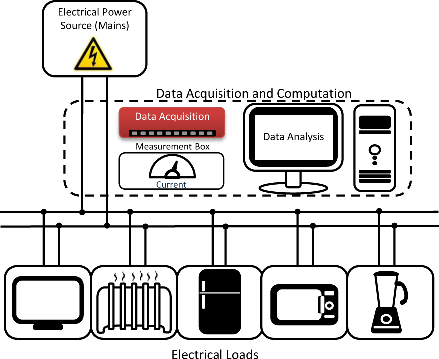
Load monitoring involves disaggregating the total power consumption of a domestic household into the appliances that are consuming power at that moment in time. The process involves analysing changes in the aggregate electrical signals of a household, for example power or current signals, and identifying what appliances are running. This allows one to know each individual appliance’s power consumption. Figure 1 shows the core components of an appliance load monitoring system. The complete system consists of the appliances that are being monitored, the electrical network to which they are connected and the monitoring system. A mix of disparate appliance Types and the non-ideal nature of the electrical supply both contribute to the challenge of designing an effective and efficient method that accurately determines the state of the system.

An appliance in its most simple form has two states: it can be either ON or OFF. However, this is not indicative of the behaviour of the majority of electrical appliances. Typically, when switched on, an appliance goes through a transitional state before it reaches its operational steady state. This can be caused by an initial spike in electrical current or by the appliance needing time to reach its operating temperature, etc. Appliances with multiple operating states add an extra dimension of complexity. Some appliances (for example, a fan heater with multiple settings) have multiple discrete states, while others (for example, a hand drill) have continuously varying states. Appliance behaviour can also be subject to user interaction. Finding a single, or small number, of meaningful electrical features that that can be used to identify all appliance is one of the challenges of load monitoring.

Studies have shown that up to 42 unique appliances contribute to the average household’s electric load, although, typically, 80% of its total power consumption can be attributed to eight appliances [6]. In a household of N appliances, there are 2^N − 1 possible different combinations of these appliances consuming power at the same time, assuming “binary” appliances. This large number of possible combinations means the load monitoring system should classify each appliance with an easily identifiable unique signature. It should be possible to identify a single appliance if it is operating alongside one or more other appliances. The cost of adding sensors and additional equipment may be hard to justify in a domestic setting, so a single point of measurement is preferable.

The voltage source in a domestic environment is not a single-frequency sine wave. It has multiple frequencies coexisting simultaneously, the amplitudes of which vary over time. This varying voltage affects each load’s current draw. In Ireland, the voltage varies between 207 and 253 V, in accordance with European Standard EN50160 [7]. The EN50160 standard also stipulates the maximum limits that the amplitudes of the higher harmonics are not allowed to exceed on the grid, which decrease as the harmonic order increases. In the test environment used in this paper, the first ten voltage harmonics have been measured to vary by up to 3% of the fundamental harmonic.

An effective load monitoring method should have a number of capabilities alongside having an acceptable degree of accuracy of identification. The computational methods used for appliance identification should have low complexity and be efficient and, so, be capable of operating in a system with large numbers of appliances. Each type of domestic appliance should be catered for, including simple resistive loads and more complex nonlinear appliances. The method should be developed with a view to being deployed on a system that uses a single cost-effective sensor and a simple data processing engine that can be deployed remotely and should be feasible to deploy in a real environment. The signature for each appliance should be sufficiently detailed to distinguish appliances with a high degree of accuracy without being overly complex or having numerous parameters. The method should not rely on large amounts of training data and should be able to cope with random variations in the environment and not be sensitive to voltage and temperature variations.

To date, there have been several load monitoring methods proposed that achieve good accuracy for appliance identification [8–20]. Accuracy is not the only metric on which the efficacy of a load monitoring technique should be measured, and when these other metrics are taken into account, there is still room to develop the methods further. These metrics include the complexity of the system and the variety and number of loads for which the method will work. The methods presented in the literature use various techniques and propose different load monitoring techniques. A thorough review of the state of the art is explored in [21,22], and some of these techniques are discussed here. One of the first load monitoring methods developed used high frequency measurements of real power (P) and reactive power (Q) for each appliance and categorised these measurements into a PQ signature space [23]. An example of a method that implements the PQ signature space uses a smart phone application to help train the algorithm and is tested for nine appliances [24]. One of the main critiques of using the PQ signature space is that similarly powered appliances are difficult to distinguish and that the method has problems in detecting multi-state and variable-load appliances. The method of using the PQ signature space has been extended by including additional signatures, for example, the instantaneous power transient profile of the appliance starting up [8–12]. This method has a good identification confidence of 87%, but is only tested for five loads, all of which are motor or electronic loads. Another example of a method that uses the PQ signature method combines this with six other signatures derived from voltage and current measurements and uses two classifiers and a committee decision algorithm to identify each appliance [19,20]. This particular method, although effective (90%), does not use actual real measurements to test their hypothesis and simulates the test data, which is not a realistic or robust test. It is also very computationally complex, has numerous signatures in the signature library and does not show the efficacy of having seven signatures over a smaller set.

Alternative load monitoring methods have been proposed that only use one signal (voltage or current) to identify appliances. An example of a method that only uses the voltage signal and a k-nearest neighbours algorithm (kNN) to identify appliances is proposed in [13]. This method uses high frequency voltage transients to identify each appliance. This method has a high identification accuracy (89%) and a short training time for each appliance. It focuses mainly on electronic and motor loads (which overall can account for approximately 45% of a domestic environment’s load consumption [25]), but does not work well for resistive heating loads (which account for approximately 25% of a domestic load). Another example of a method that uses one electrical signal to identify appliances uses fifteen odd fast Fourier transform (FFT) current harmonic amplitudes and a neural network to identify appliances [15]. This method achieves a confidence of approximately 80% for eight to ten appliances, but has high complexity and is not tested for a wide enough range of appliances.

Some load monitoring methods proposed use simple power measurements and model the appliances using more complex models, for example hidden Markov models [17,26]. The algorithm creates appliance models that describe specific appliances using characteristics, such as the behaviour of the appliance, for example time of use or length of usage. This method has been tested and trained for specific “large consumer” appliances, such as fridges, dishwashers, etc., but has not been tested for smaller household loads.

Table 1. Comparison of complete load monitoring techniques.

Method	Loads	Breakdown of Test Loads	Data Used	Confidence	Complexity
Real and reactive power (PQ) values for each appliance at the start and end of runtime and a nearest neighbor classifier with Euclidean distance [24].	8	Tested for ohmic, inductive and capacitive loads. Does not work for variable appliances.	Fs = 1 kHz Training: three events per appliance Testing: 144 random events of different combinations.	87%	N
Instantaneous power transient profile and PQ steady state with a neural network [8–12].	5	Motor and electronic loads. Unknown appliances not considered.	Fs = 30 kHz Training: 13 events per appliance Testing: same as training	87%	N + N2
High frequency noise on voltage line and a k-nearest neighbour (kNN) classifier [13,14].	10–20 per seven houses	Detects electronic loads, cannot detect resistive loads. Unknown appliances not considered.	Fs = 1 MHz Training: 1 event per appliance Testing: 2576 events	89%	N
Fifteen harmonics from the Fourier transform of the current and a neural network [15].	8–10	Tested for a selection of loads, mainly electronic loads. Unknown appliances not considered.	Training: 18 readings per appliance (10 s apart) Testing: 18 readings for each of the 256 combinations	70%–86%	2N
Hidden Markov models are used to model each appliance based on observations, and the total power is disaggregated using these models [16–18].	5	Trained for large consumer loads. Unknown appliances have no effect.	Training: 30 min per appliance in isolation Testing: 120 events of 10 combinations	90%	N
Seven different signatures (derived from voltage and current) with a least residue, a NN classifier and three committee decisions; a maximum likelihood estimator (MLE), a least unified residue (LUR) and a most common occurrence (MCO) [19,20].	27	Tested for a large selection of load Types. Unknown appliances not considered.	Fs = 12.8 kHz Training: Each appliance is measured in isolation Testing: combinations are mathematically created	MLE: 90% LUR: 85% MCO: 83%	N

offers a comparison of the methods described above. These methods are analysed by the differences in their approach, the input data required by the method (e.g., voltage, current, sampling rate), the testing regime used (e.g., number of appliances) and the computational complexity of the algorithm used. From the current research, questions still remain on load monitoring and the best practices. Our main goals of a low complexity algorithm that can scale to many appliances has good accuracy in differentiating particularly between resistive loads and verification of this using multiple resistive appliances in the test set, but does not align well with these proposed algorithms. For these reasons, it would be difficult to construct a fair comparative test, and therefore, a comparison is offered through Table 1. This research aims to provide a solution that addresses all of the criteria for an effective load monitoring solution. The method proposed in this paper is event based, and the complexity of the algorithm is low (of order N, the number of appliances). It is optimised to work for all varieties of appliances found in a domestic setting and retain an acceptable accuracy (> 0:8).

The method proposed in this paper detects power ON/OFF events, and then, features from both the time and frequency domains are extracted from the current signal from around this event and are used to identify the appliance. These features consist of parameters from the temporal transient signal, which represent the rate of change of the current, and parameters from the steady-state current in the frequency domain, which are derived from the current harmonics. A library of features is built for each appliance during a training period by sampling the switch ON transients and the current harmonics in the steady state for each appliance in isolation. The current is then continuously sampled, and when an event occurs, the features are extracted from this event to identify the appliance, using a two-step classification algorithm. The rest of the paper is laid out as follows. Section 2 outlines the motivation for the algorithm design. Section 3 describes the method in detail. Section 4 describes the experiments carried out. Section 5 presents the results, and the paper is concluded in Section 6.

2. Motivation for Algorithm Design

2.1. The Differences between Different Load Types

The method proposed in this work is tested for a set of loads, each of which has different electrical components and characteristics (

Table 2. Properties of the set of test appliances, as measured by the Allegro PM3000a Universal Power Analyser at 50 Hz.

Appliance	Average Power (W)	Resistance (Ω)	Reactance (Ω)	Power Factor
Panel radiator	320	160	0.005	1.000
Fan heater	1790	30	0.260	1.000
Kettle	1975	30	0.005	1.000
Grill	1300	42	−0.400	1.000
Hairdryer	1720	31	0.031	1.000
Refrigerator	120	460	150.1	0.947
Blender	365	230	34.0	0.997
Vacuum cleaner	1360	42	6.9	0.982
Microwave	1710	50	3.3	0.998
Ceiling lights	280	186	−1.5	0.999
Halogen bulb	50	1086	−9.0	0.995
PC	200	718	−40.0	0.997
LCD television	190	419	−113.5	0.949
Laptop	130	1684	−119.4	0.997
LCD Monitor	110	1546	−650.0	0.890

). The appliances chosen for this test represent a typical household and are based on a survey carried out in 251 different houses over the course of a year [25]. The majority of loads in households tend to be resistive heaters (kettle, oven, storage heating), or have a motor (refrigerator, blender, water pump), or are electronic loads that have a switched mode power supply (SMPS) (laptop, television). Appliances that have heating elements contribute to over 25% of typical domestic power consumption, so five representative loads have been chosen for this test; similarly, loads with a motor account for 25%, lighting accounts for approximately 10% and electronic loads for 15% [25]. These different categories of loads will have general trends in terms of reactance; i.e., resistive heating loads will have very small to negligible reactance, motor loads will have inductive reactance (due to the coil in their stator) and lighting loads, specifically halogen bulbs, are capacitive. Table 2 shows the set of appliances selected to test our proposed method, each of which fit into one of the four load categories listed. Included are the measured resistance, reactance (positive and negative representing inductive and capacitive) and power factor for each appliance.

In order to identify each appliance, an appliance signature is derived from the electrical signal of each appliance. The signature library should uniquely identify each appliance. The Fourier transform of a signal transforms the waveform from the time domain into a sequence of values at different frequencies in the frequency domain. The current spectra were found to be different for each appliance. From our empirical tests, it has been found that for the set of appliances used in the test that the first three odd harmonics of the spectrum give a sufficient approximation of the signal and distinguish each appliance. This choice is supported by the harmonic limits stipulated in EN61000-3-2 (

Table 3. EN61000-3-2 current harmonic limits for two classes of household appliances. Class A appliances are household appliances up to 16 A, and Class D appliances are electronic appliances that are rated less than 600 W. The limits for the even harmonics of Class D appliances are not specified by the standard.

	Current Limit (A)
Harmonic Order	Class A	Class D
2nd	1.08	–
3rd	2.30	2.30
4th	0.43	–
5th	1.14	1.14
6th	0.30	–
7th	0.77	0.77
8th	0.23	–
9th	0.40	0.40
10th	0.18	–
11th	0.33	0.33
…	…	…
n-th	$0.15\left(\frac{15}{n}\right)$	$0.15\left(\frac{15}{n}\right)$

). If these limits are met by appliance manufacturers, there should be very little harmonic content in the even current harmonics, and as the frequency spectrum increases, the amplitudes of the odd current harmonics also should decrease [27].

There are three different Types of electrical loads evident in the test set, linear nonreactive loads (for example, heating loads like radiators or kettle), linear reactive loads (for example, halogen bulbs) and nonlinear reactive loads (for example, refrigerator, PCs, etc.).

Table 4. The mean of the amplitude of the current harmonics for each appliance used in this experiment.

Appliance	First Harmonic	Third Harmonic	Fifth Harmonic
	(50 Hz)	(150 Hz)	(250 Hz)
Panel radiator	1.314 A	1.60%	1.57%
Fan heater	7.440 A	1.05%	2.28%
Kettle	8.229 A	0.92%	2.07%
Grill	5.414 A	1.05%	2.09%
Hairdryer	7.150 A	0.79%	2.51%
Refrigerator	0.402 A	13.40%	3.90%
Blender	1.255 A	21.56%	1.96%
Vacuum cleaner	5.140 A	11.14%	1.15%
Microwave	4.998 A	30.86%	10.49%
Ceiling lights	1.190 A	0.70%	1.45%
Halogen bulb	0.202 A	0.80%	1.98%
PC	0.294 A	85.82%	61.91%
LCD television	0.530 A	38.19%	1.84%
Laptop	0.169 A	86.95%	66.46%
LCD Monitor	0.344 A	11.89%	16.16%

shows the mean FFT harmonic amplitudes measured for each appliance in this test. These values were obtained using a sampling frequency of 20 kHz and applying a Hanning window.

When analysing the current FFT with the intention of creating an identifiable signature library, the load type and its characteristics are to be taken into account. Which harmonics have useful information for the purpose of identifying an appliance depends on the type of load. Linear nonreactive loads do not generate harmonics of their own. The current harmonics exhibited by linear nonreactive loads are a reflection of the voltage harmonics and scaled by their unchanging impedance. Linear reactive loads do not generate harmonics of their own, but their impedance changes at each harmonic with respect to the frequency. The impedance of the load changes at each harmonic, and therefore, each harmonic gives additional information about the load. Nonlinear loads contain circuit components that distort the voltage waveform and generate their own harmonic currents, in addition to the harmonics already present in the voltage supply waveform. The measured reactance is shown in Table 2, and it can be seen that, depending on the type of load, the reactance values vary. Linear nonreactive loads have a very low measured reactance (< 1 Ω), whereas linear nonreactive and nonlinear loads have a higher reactance than this. The power factor is also different for these different Types of loads; it is equal to one for nonreactive loads and less than one for reactive loads.

There is a significant distinction between the harmonic content for the linear nonreactive loads (the first five loads) and the nonlinear loads (the remainder of the loads excluding the two lighting loads) (Table 4). Reactive loads filter and attenuate the voltage harmonic content, for example the third harmonic of the ceiling lights and halogen bulb are lower than any other appliance. Due to the low harmonic content of linear nonreactive loads and it being mostly a reflection of the voltage, this would suggest that using these harmonics would add a source of noise, the voltage source variation. The nonlinear loads have high harmonic content. It is for this reason that the appliances are separated into two different Types, where Type I loads are linear nonreactive loads and Type II are nonlinear loads and linear reactive loads. A steady-state characteristic of a Type I load is that the inherent signal information in contained in the fundamental harmonic, and the higher harmonics are simply a reflection of the line voltage harmonics at that point in time. Contrastingly a steady-state characteristic of a Type II load is that the higher harmonics contain information that is inherent to the appliance. Therefore, when classifying the appliances, Type I loads should only use the fundamental harmonic and Type II should use all of the harmonic content.

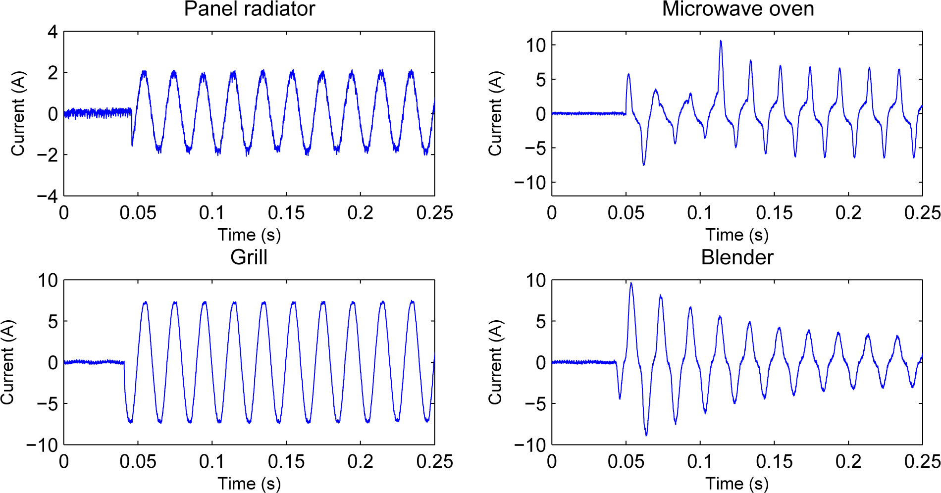
In order to differentiate between the two types of appliances, a second characteristic of each load type is needed; this is where the transient signal applies. When an appliance turns ON, it has a unique transient signal. This signal can inform about the overall reactance of a load and whether it is purely resistive or has an overall inductive or capacitive reactance. This characteristic is tied to the type of appliance and, therefore, the steady-state characteristics of the load. This work assumes that all nonlinear loads are reactive, and so, the transient can be used to distinguish between Type I and II loads. Figure 2 shows the start-up transient signal for four different loads, each belonging to one of the two load types, a radiator (Type I), grill (Type I), a microwave (Type II) and a blender (Type II). Type I loads, due to the characteristics of a linear nonreactive load, have no associated transient. When the appliance turns on, it immediately enters steady-state operation with no “inrush” or “suppression” of the starting current. Type II loads do have an inrush or suppressed starting current due to the nature of reactive and/or non-linear loads. This transient signal information can be used to differentiate between the two load types at start up.

2.2. The Naive Bayes Classifier

Classification is the problem of identifying to which class a new observation belongs. Each class is described by its features. The classifier used to identify each appliance in this method uses a naive Bayes classifier. In this case, an individual appliance is the class, and the features are the amplitudes of the first three odd current harmonics. The naive Bayes classifier was chosen as it can be rapidly deployed within a system [28]. It is an appealing classifier because of its simplicity, robustness and surprising effectiveness [29]. The classifier can be readily applied to huge data sets, and the results are easy to interpret. An advantage of the naive Bayes is that it only requires a small amount of training data to estimate the parameters necessary for classification. The classifier is based on Bayes’ theorem and assumes independence between the individual features, and because independent variables are assumed, only the variances of the features for each class need to be calculated [28,29]. Although the classifier assumes independence between the individual features, it has been shown that the naive Bayes classifier may still be optimal, even when there are strong dependencies present between the attributes [28,30].

Some work has been carried out in the literature to compare different algorithms for load monitoring. Marchiori et al. [31] compared a maximum likelihood classifier with a naive Bayes classifier using the PQ signature space. They found that the naive Bayes classifier performed better. Reinhardt compares a total of nine different classification methods, including a Bayesian network, a naive Bayes, a random forest and random committee method [32]. They find the Bayesian network the most favourable method for their signature, with the naive Bayes classifier as a very close second (0.03% difference in accuracy). It is for these reasons that the naive Bayes classifier was chosen as the classifier in our method.

3. The Load Monitoring Method

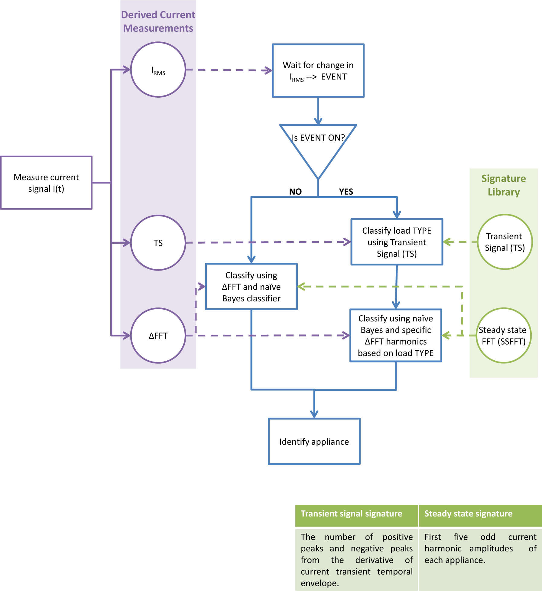
A flow diagram of the proposed algorithm can be seen in Figure 3. The method waits for an appliance to turn ON or OFF; this is identified as an event. The algorithm deals with ON and OFF events differently. In the case of an ON event, the algorithm uses characteristics from the current signal in both the temporal and frequency domains to identify each appliance. In the case of an OFF event, the algorithm identifies the appliance using characteristics from the current signal in the frequency domain only.

By tracking what appliance has caused each event, the algorithm can identify what appliances are consuming power at any time. There are three parts to the appliance identification algorithm: the event detection, the classification of the load type and the specific appliance identification.

3.1. Event Detection and the Extraction of the FFT Signature of an Event

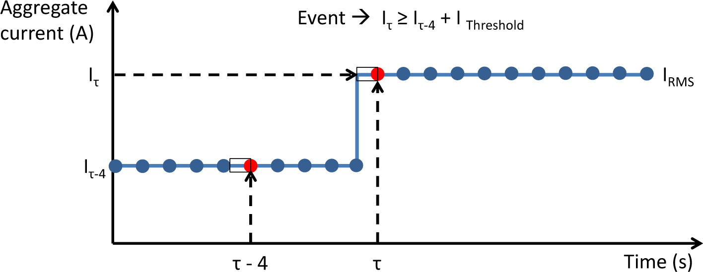
The event detection is based on a moving window that identifies changes in the root mean squared (RMS) current amplitude. A one-second array of current signal samples contains fifty wavelengths (at 50 Hz). The RMS current is calculated from this array every second. There are two criteria that must be met in order for an event to be identified. The first criterion is that the absolute magnitude of the RMS current signal at this time now must be greater by a threshold value (75% of the smallest appliance’s current) than the RMS current signal four seconds before. The second criterion that must be fulfilled is that the previous event detected must not have occurred in the last three seconds. This avoids parts of the same transient signal being detected as spurious events. A four-second window was chosen in order to allow for appliances with long start up signals. This allows the appliances enough time to settle into the steady state. This also adds the limitation to the algorithm that events that occur within three seconds of each other will not all be identified correctly. If these criteria are met, an event has been detected (Figure 4). The event is labelled ON or OFF depending on the direction of the change in magnitude.

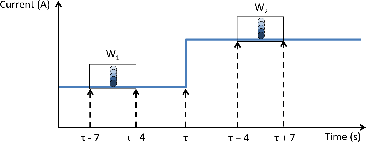
Once an event has been detected, the difference in the FFT harmonic amplitudes (ΔFFT) before and after the event is found (Figure 5, Equation (2)). The windows before (W₁) and after (W₂) the event are selected, and the first three odd harmonic amplitudes are calculated from each (Equation (1)). The windows are selected from [τ – 7, τ − 4], before the event and [τ + 4, τ + 7] after the event. The window is chosen four seconds after the event occurs in order to allow the appliance to reach the steady state:

$$I_{ff{t}_{W1}}={\displaystyle \sum _{n=\tau -7}^{N=\tau -4}{i}_n{e}^{-2\pi k\frac{n}{N}},k=1,3,5}$$

(1)

$$\mathrm{\Delta }FFT=\left|I_{ff{t}_{W1}}-I_{ff{t}_{W2}}\right|$$

(2)

3.2. Signature Library

The signature library contains parameters that represent each appliance. For each appliance, there are twelve parameters; these parameters represent feature characteristics of each appliance. The parameters are derived from the training data. There are two sets of parameters; one set represents steady-state characteristics and the other, transient characteristics.

Table 5. An example entry in the signature library for two appliances (one of each type).

Appliance	Steady-state signal	μFFT50	μFFT150	μFFT250
		σFFT50	σFFT150	σFFT250
	Transient signal	NTSpp	NTSnp
Kettle	Steady-state signal	8.229 A	0.076 A	0.170 A
		0.030 A	0.002 A	0.004 A
	Transient signal	1.7	0.0
Refrigerator	Steady state signal	0.402 A	0.055 A	0.014 A
		0.023 A	0.003 A	0.002 A
	Transient signal	1.4	4.7

shows an example entry in the signature library for two appliances. Each individual appliance’s signature is generated from that appliance operating in isolation in the steady state. The first three odd harmonics are sampled for a training time, and the mean μ_FFT and standard deviation σ_FFT of each are calculated and are used as the signature parameters. Each appliance is measured in isolation and switched ON and OFF several times. The steady-state signal then takes a set amount of time after each transient occurs and records for a specific length of time. This steady-state data were then used to calculate the mean and standard deviation used as signatures for each appliance.

The transient signal is represented by two values in the library that denote the rate of change of the current signal at start up. When an appliance turns ON, the current signal undergoes a transient state before it reaches the steady state. This transient signal can be seen as a step response and gives information about the reactance of the electrical appliance that has just turned ON. In our method, the transient signal is characterised by its rate of change. The positive profile of the transient signal is calculated from the maximum peak values from each waveform period. The derivative of the positive profile is calculated, and the peaks in the derivative above and below a threshold represent the rate of change of the transient signal. If there are no negative peaks in the derivative, this means that there is not an overshoot in the transient signal, and the appliance’s transient signal is not capacitive. To create the signature library, each appliance was switched ON several times. The transient signal was captured, and the number of positive peaks N_TSpp and negative peaks N_TSnp in the derivative were counted. The average of these counts are given in

Table 6. The library values representing the rate of change of the transient signal.

	Appliance	Positive Peaks NTSpp	Negative Peaks NTSpp
Type I	Panel radiator	1.6	0.4
	Fan heater	1.9	0.0
	Kettle	1.7	0.0
	Grill	1.3	0.0
	Hairdryer	1.8	0.7
Type II	Refrigerator	1.4	4.7
	Blender	1.2	13.9
	Vacuum cleaner	1.2	3.7
	Microwave	6.3	11.6
	Ceiling lights	1.0	3.7
	Halogen bulb	1.5	5.2
	PC	1.3	4.6
	LCD television	2.2	4.6
	Laptop	0.9	2.4
	LCD Monitor	2.8	7.6

.

It can be seen that the Type II appliances have multiple negative peaks in the rate of change of their transient signal. For the Type I appliances, this is not the case. From the data recorded in the signature library, it was decided that if the number of positive peaks in the transient signal were equal to one or two and there were no negative peaks in the transient signal, the appliance was Type I. Otherwise, if these criteria were not met, the appliance was Type II. This information from the signature library is used to identify the load type in the first step of the algorithm.

3.3. Step One: Classify Load Type Using the Transient Signal

When an ON event is detected, the algorithm classifies whether the appliance is Type I or II from the rate of change of the transient signal. The load’s type effects how it is treated by the next classification step.

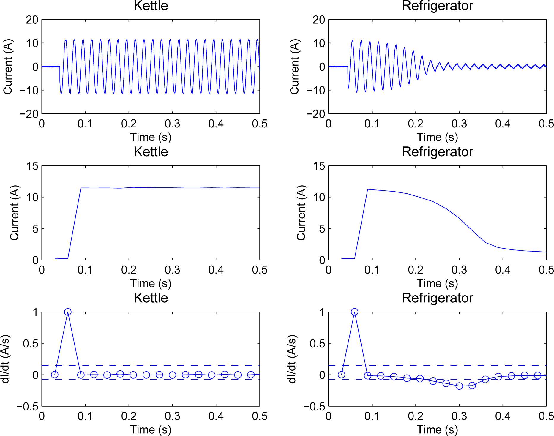
When an ON transient signal is detected, the positive profile of the signal is calculated. Figure 6 shows an example of the transient signal of a Type I appliance (kettle) and a Type II appliance (refrigerator). The first row of the figure shows the temporal transient current signal of each appliance. The second row shows the positive profile of the transient signal, which is derived from the maximum peak value from each period of the transient signal in a 40 ms window. The derivative of this envelope is calculated and normalised to lie between −1 and 1. Then, the numbers of positive and negative peaks in the transient profile derivative above and below certain thresholds are counted. An upper threshold of 0.15 and a lower threshold of −0.075 were chosen from tuning the algorithm using the transient signals collected from the training data. These thresholds were chosen, as the first (positive) rate of change tended to be of more significance than any other rate of change within the derivative, and in general, the positive rates of change tended to be more significant than any of the negative rates of change. In order to capture some of the smaller deviations for some of the Type II appliances, a smaller negative threshold was needed.

Figure 6 shows the difference between two different types of loads. For the Type I appliance’s derivative, it can be seen that there is only one positive peak that lies outside the boundaries. The Type II appliance has one positive peak and six negative peaks that lie outside the boundaries. Table 2 shows a reactance of 0.005 Ω for the kettle and 150.1 Ω for the refrigerator at 50 Hz. The refrigerator has a capacitive reactance at start up, and this is visible through the inrush current in the transient signal. The overall reactance of the kettle is quite small (almost negligible), and this is clear from the lack of transient signal when the appliance turns ON. For all Type I appliances, there are one or two positive peaks and no negative peaks in the derivative plots. For all Type II appliances, there is at least one negative peak in the derivative.

There is no classification of type carried out for OFF events. When an appliance turns OFF, there is no transient signal associated with the turn OFF. For this reason, there are no extractable features from an OFF event and no way of classifying the load type using the current transient signal.

3.4. Step Two: Classifying the Appliance Using Steady-State Signal and Naive Bayes Classifier

The naive Bayes classifier uses training data to calculate signature distributions for each appliance. The signatures for each appliance are the amplitudes of the first three odd current harmonics. The prior probability is the probability before any evidence is taken into account. It is assumed that each appliance A_j is equally likely to be switched ON at any time, so the prior probability is the same for all appliances (Equation (3)), where N is the number of appliances and j is the appliance 1:N. The calculated difference in the harmonic amplitudes (ΔFFT; Figure 5) from before and after an event are input to the classifier, and the probability for that value belonging to each individual appliance is calculated. The appliance with the highest probability is chosen as the most likely appliance to have caused that event:

$$P(A_j)=\frac{1}{N}$$

(3)

Each appliance A_j is represented in the library by three harmonics, and each harmonic is a normal distribution H_i ~ N(μ_i, σ_i), where i is one of the harmonics. The mean μ_i and standard deviation, σ_i for each distribution are calculated from training data. The algorithm is fed a test sample $\overline{x}$ (i.e., ΔFFT), where the values for each of the harmonic amplitudes are known, but the appliance is unknown. The sample $\overline{x}$ is a vector that contains three values, each representing a current harmonic amplitude at a point in time. The probability that $\overline{x}$ belongs to appliance A_j is calculated, using the harmonics from $\overline{x}$ and the distributions for A_j from the signature library. The probability is calculated for each of the harmonics from test sample $\overline{x}$ to belong to a specific harmonic distribution (Equation (4)):

$$p\left(x_i|H_i\right)=\frac{1}{\sqrt{2\pi {\sigma }_i^2}}\exp \left(\frac{-{\left(x_i-{\mathrm{\mu }}_i\right)}^2}{2{\sigma }_i^2}\right)$$

(4)

It is assumed that for each appliance, the harmonics are independent. The product of the harmonic probabilities for each appliance is calculated (Equation (5)). This probability is known as the likelihood, which is the probability of the sample $\overline{x}$ belonging to A_j:

$$p\left(\overline{x}|A_j\right)={\displaystyle \prod _{n=1}^{3}p(H_i|x_i)}$$

(5)

The algorithm calculates the posterior probability that $\overline{x}$ belongs to each of the appliances A_j (for example, the refrigerator, radiator, etc). The adjusted probability (posterior) is $p\left(\overline{x}|A_j\right)$, which is the probability that the sample $\overline{x}$ belongs to A_j, given the features of the class A_j. The posterior probability is calculated in Equations (6) and (7), where the prior is the probability of a specific appliance switching on. The likelihood is the probability that the features of $\overline{x}$ belong to A_j. The evidence is a summation of the likelihoods of the sample $\overline{x}$ belonging to any of the appliances. The evidence is then used as a scaling factor to have the posterior lie between zero and one:

$$\mathit{posterior}=\frac{\mathit{prior}\times \mathit{likelihood}}{\mathit{evidence}}$$

(6)

$$\mathit{posterior}(A_j)=p\left(A_j|\overline{x}\right)=\frac{P(A_j)\times p\left(\overline{x}|A_j\right)}{{\displaystyle {\sum }_{n=1}^{N}P(A_k)\times p\left(\overline{x}|A_k\right)}}$$

(7)

The posterior probability is calculated for all of the appliances in the library. The maximum calculated posterior from all of the appliance posteriors is then identified as the most likely appliance to be consuming power.

When an event occurs, the differences in the FFT amplitudes before and after the event are found, (ΔFFT); these differential amplitudes are used to identify the appliance. In the appliance test set, there are five Type I appliances and ten Type II appliances. If the appliance has been classified as a Type I load, the fundamental FFT amplitude and the fundamental harmonic signatures of the five Type I appliances are input to the naive Bayes classifier. Similarly, if the appliance is identified as Type II, the three FFT amplitudes are input to the naive Bayes classifier alongside the ten Type II appliance signatures. The most likely appliance is identified from the appliance with the highest probability from the classifier.

When the event is OFF, there are no transient features associated with the signal and there is no classification of the type step. In this case, the difference before and after the event is found for all FFT harmonics of the measurement signal and with all fifteen appliance signatures as input to the naive Bayes classifier. The most likely appliance to have caused the event is identified.

4. Experimental Procedure

In order to assume a realistic training time for a real environment deployment, it was attempted to keep the training time for each appliance to a minimum. Each appliance was measured in isolation. The appliance under test was switched ON ten times to record the transient signal. The steady-state signal was measured from five seconds after each transient and recorded for a further ten seconds. For each appliance, there was a total of 100 s of steady-state data to create the steady-state signatures and ten transient events from which to derive the transient signatures. All of the training data for all of the appliances was recorded over a three-hour period.

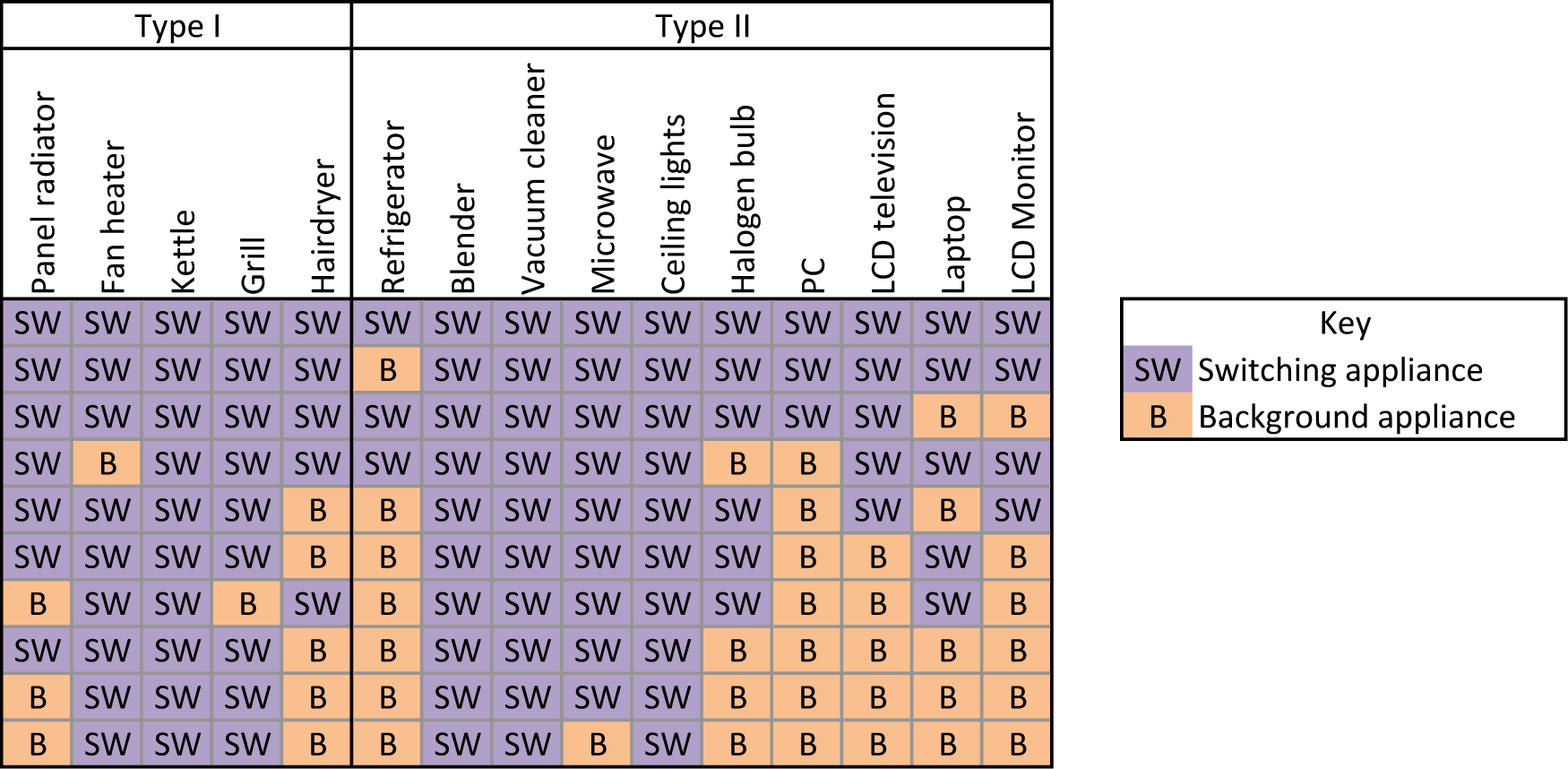
There are fifteen different test appliances, which means there are over 32,000 (2^N − 1) unique combinations of the different appliances being switched ON and OFF. It is not possible to record all of these combinations. In order to attempt to have a stringent, robust test, each appliance was power cycled a number of times under different conditions. Initially, each appliance is tested individually and then tested while other appliances are operating in the steady state. The appliance under test was power cycled, while combinations of up to nine other appliances were operating in the steady state. Figure 7 shows a breakdown of which appliances were switched and which appliances were used as background appliances in each set of tests. Each row in the figure denotes one set of experiments; the first row has no background appliance, and each appliance is tested in isolation; the second row has one background appliance (the refrigerator), and fourteen appliances are power cycled while it runs, and so on. There were a total of 758 events recorded. Each appliance was turned ON for between thirty seconds and a minute and then turned OFF.

To ensure sufficient data were collected to test the algorithm fully, different appliances were used as background appliances, while others were tested as switching appliances. In general, the appliances chosen as background appliances for each test tend to be those that would be found operating over longer periods of time as background appliances in a household, for example the PC, LCD television or the refrigerator. The switching appliances chosen in this test also tend to be appliances that are switched on for shorter periods of time, while other appliances are operating, for example the kettle or the blender.

4.1. Experiment Equipment

The current is measured using a 20 A Allegro Hall Effect ACS712 sensor (Allegro Microsytems LLC, Worcester, MA, USA) that has an 80-kHz bandwidth [33]. This current sensor is electrically isolated from the mains and outputs a voltage between 0 and 5 V. The signal is recorded in the temporal domain at a sampling frequency of 20 kHz. The sensor has a total output error of 1.5% at 25°C; the sensitivity of the sensor is typically 100 mV/A, and the sensor noise is 11 mV. The current is read using a LabJack UE9 DAQ (LabJack Corporation, Lakewood, CO, USA) [34]. The LabJack has a dual-processor with 168 MHz processing power and a USB 2.0 interface. Each input has a 0–5 Volt range and a 12-bit resolution. The measurements are all taken at room temperature.

5. Results and Analysis

To ensure that the classification algorithm that is used has a high degree of confidence, a calculation to assess its performance is carried out. This is done by comparing the output results of the classifier with its expected targets. For the purpose of this work, and as mentioned in [21], a receiver operating characteristic (ROC) curve is used to test the effectiveness of the algorithm. The ROC curve [35] illustrates the performance of a binary classifier system by identifying the true positives, true negatives, false positives and false negatives. The ROC curve is the fraction of true positions out of positives plotted against the fraction of false positives out of negatives or the true positive rate (TPR) versus the false positive rate (FPR). A common method to compare classifiers is to plot the ROC curve calculate the area under the curve (AUC). The AUC’s value will always be between 0 and 1. If a classifier randomly guesses the positive class half of the time, it can be expected to get an AUC value of 0.5; therefore, a realistic result from a classifier should be above 0.5. As there are three parts to the algorithm, there are three stages at which the accuracy of the method has to be calculated; the event detection; appliance type classification; and the specific appliance identification.

5.1. Accuracy of Event Detection

The overall accuracy of event detection was 0.903 (

Table 7. Accuracy of the event detection algorithm.

Description	Value
Total number of events	758
Number of detected events	701
True positive rate	0.890
False positive rate	0.084
Accuracy	0.903

). The accuracy is calculated from the total number of true positives and true negatives out of all of the positives and negatives detected by the event detection algorithm. Perfect event detection will have a TPR of one and an FPR of zero; in this case, the event detector has a TPR of 0.890 and an FPR of 0.084.

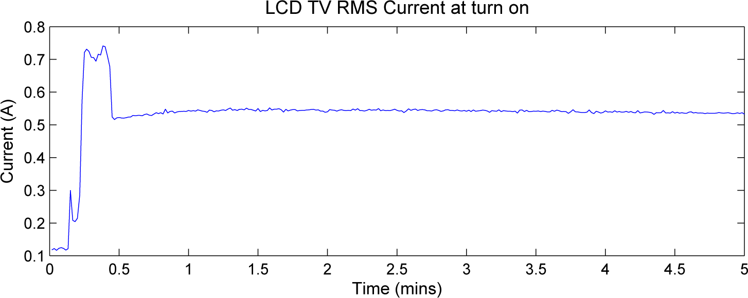
The accuracy of the event detector was spread evenly across all appliances, apart from the halogen lamp, which had an overall accuracy of detection of 0.670. This was lower than other appliances due to its low power consumption and its small transient signal. The threshold values chosen for the event detection could be changed to improve the halogen lamp’s accuracy. Changing this would have an effect on other appliances, specifically the television, where extra non-events would be captured. Figure 8 shows the RMS current of the television when it turns on. It can be seen that it has an initial state that lasts for thirty seconds and then a drop in current, which would be identified as an OFF event if the threshold values were changed. It was for this reason that the poor accuracy of the halogen lamp’s events was accepted.

5.2. Accuracy of Type Classification

The average AUC calculated for the classification of the appliance type using the transient signal is 0.936, which is shown per appliance in

Table 8. Area under the curve (AUC) values for classifying the correct type to an appliance based on features from the ON transient signal.

	Appliance	AUC
Type I	Panel radiator	0.697
	Fan heater	0.989
	Kettle	0.973
	Grill	0.973
	Hairdryer	0.967
Type II	Refrigerator	1.000
	Blender	1.000
	Vacuum cleaner	0.700
	Microwave	0.963
	Ceiling lights	0.857
	Halogen bulb	1.000
	PC	1.000
	LCD television	0.931
	Laptop	1.000
	LCD Monitor	0.969

. The threshold values chosen in the algorithm were optimised to work across all appliances.

Most appliances have a very good AUC (> 0:85). The radiator and vacuum cleaner have the worst performance. The vacuum cleaner’s transient has a slow rate of decay, and therefore, sometimes, the peaks in the derivative of the envelope fall below the threshold values. The radiator shows a low frequency oscillation (10 Hz), which sometimes falls above the threshold values. This oscillation could be due to the thermal lag of the appliance and the effect of the changing temperature on the resistance. The thresholds were optimized in order to have an acceptable classification accuracy for both of these appliances.

5.3. Accuracy of Appliance Identification

Once an event has been detected, the specific appliance is to be classified. The first table in this section classifies all of the appliances with the same set of features. There is no type classification in this table.

Table 9. AUC for identifying an appliance when using two different feature sets.

	Appliance	Fundamental Harmonic	First Three Odd Harmonics
Type I	Panel radiator	0.681	0.545
	Fan heater	0.873	0.613
	Kettle	0.929	0.689
	Grill	0.583	0.537
	Hairdryer	0.812	0.642
Type II	Refrigerator	0.809	0.951
	Blender	0.936	0.965
	Vacuum cleaner	0.784	0.855
	Microwave	0.966	0.988
	Ceiling lights	0.792	0.894
	Halogen bulb	0.795	0.952
	PC	0.710	0.983
	LCD television	0.667	0.796
	Laptop	0.788	0.949
	LCD Monitor	0.528	0.667

shows the results of using specific harmonics amplitudes for identification. The method uses an event detection to find an event. The naive Bayes classifier is then used with either one or three current harmonics to identify the appliance. It can be seen that using just the fundamental harmonic for Type I appliances is best, whereas using the first three odd harmonics is better for identifying all of the Type II appliances. This is due to the higher harmonics containing extra information for Type II appliances and redundant information for Type I appliances. This compounds the concept of classifying the appliance type first. The results of using the type classification combined with a specific number of harmonics can be seen in

Table 10. AUC calculated for identifying an appliance turning ON and OFF when classifying the type based on the transient signal and then using a select set of current harmonics as features based on the type.

	Appliance	Total AUC	On AUC	Off AUC
Type I	Panel radiator	0.576	0.624	0.544
	Fan heater	0.733	0.861	0.606
	Kettle	0.805	0.923	0.693
	Grill	0.703	0.887	0.519
	Hairdryer	0.722	0.821	0.623
Type II	Refrigerator	0.951	0.961	0.939
	Blender	0.965	0.972	0.969
	Vacuum cleaner	0.764	0.679	0.960
	Microwave	0.975	0.962	0.987
	Ceiling lights	0.912	0.930	0.894
	Halogen bulb	0.954	0.982	0.926
	PC	0.983	1.000	0.967
	LCD television	0.766	0.783	0.955
	Laptop	0.949	0.967	0.930
	LCD Monitor	0.667	0.638	0.708

.

As the first classification step only works at ON transients, the results in Table 10 are divided into ON and OFF events to compare the performance in greater detail and to see the improvement more clearly. There will be no improvements in the OFF events as, if the event is OFF, the method uses all three odd current harmonic amplitudes to identify the appliance due to no OFF transient signal. The percentage classified as the correct type is quite high (Table 8), so this high confidence allows the set of possible appliances to be reduced, i.e., if the load type is classified as Type I, there are only five possible candidate appliances, and vice versa. This adds additional improvement to the method when the correct type is classified, but it also results in disimprovement for the appliances whose type is not classified correctly. It is expected that, overall, the method should show an improvement compared to using only one or three current harmonic amplitudes. This improvement will be visible in the ON events, specifically the Type I appliances.

All Type I appliances show an overall improvement compared to using the three odd current harmonics (Table 9, Column 2). They also show an improvement compared to using the fundamental harmonic. This is due to the reduction of possible appliances through classification of appliance type, as there are only five possible Type I appliances in the set. This improvement is particularly noticeable in the ON events. In nearly all cases, the Type II appliances retain their high accuracy of prediction, as seen in Column 2 of Table 9. The vacuum cleaner does not, due to its lower accuracy of 0.7 when classifying type (Table 8). The vacuum cleaner is an example of an appliance for which type is not always classified correctly. This means that when the appliance type of the vacuum cleaner is incorrectly identified as Type I, the vacuum cleaner is then misidentified by the naive Bayes classifier as one of the Type I loads. This is the reason for the accuracy of the identification of the vacuum cleaner being lower for ON events than OFF events in Table 10. Similarly, the LCD monitor also has a lower accuracy than the previous method of just using the three odd current harmonics for all appliances, and its classification of type is also a little bit lower than the other Type II appliances.

5.3.1. Effect of Background Appliances

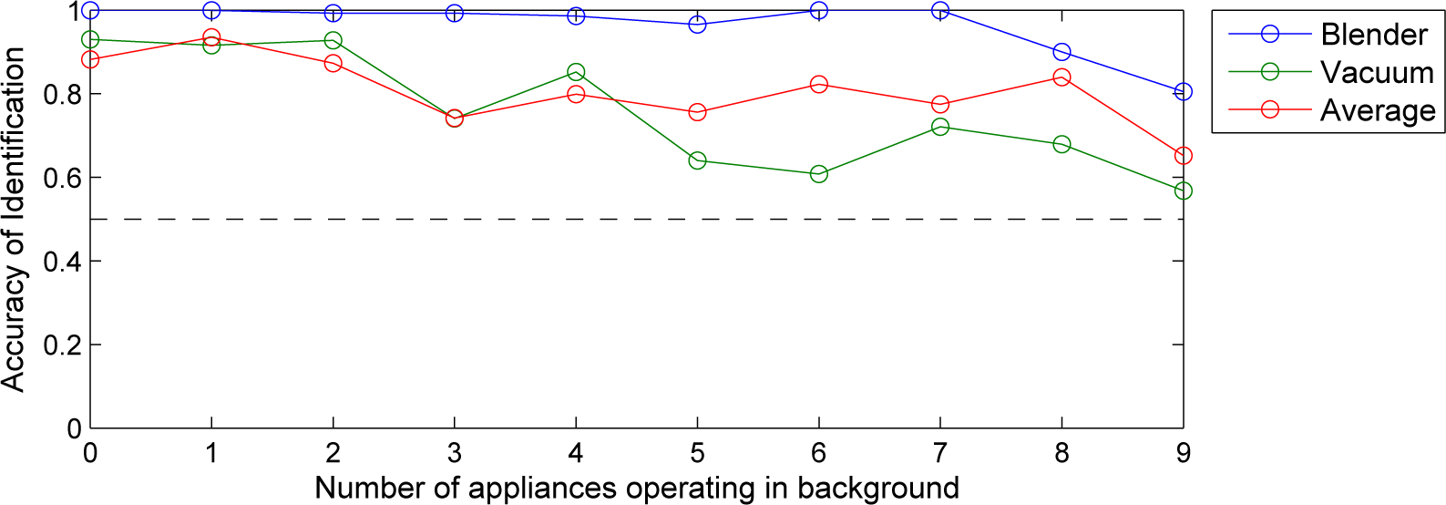
One experiment carried out was to examine the effect on the algorithm’s accuracy of identification as more appliances operated in the background. The overall trend of the algorithm’s accuracy is to decrease as more appliances are switched on in the background. This is to be expected, as when more appliances are operating in the background, it adds more noise to the system. This affects appliances at different rates. Figure 9 shows the accuracy of the appliance identification as more background appliances (zero to nine) are switched on. Not all appliances are effected at the same rate, as can be seen in the graph. The blender has a better performance when more appliances are switched on than the vacuum cleaner. The blender and vacuum cleaner can be seen as an example of best and worst case performances, the average performance of the vacuum cleaner being 0.76 and the blender being 0.97.

Not every single combination of background appliances was tested in each set of background appliances, and not every appliance was tested for each set (Figure 7). This should be taken into account when looking at the average accuracy. For example, in the last test, the appliances used as the switching appliance in the last test (fan heater, kettle, blender, grill, vacuum cleaner and ceiling light) are the lower accuracy appliances; therefore, overall, the average accuracy will drop in that case.

6. Conclusions and Future Work

This paper presents a method that identifies appliances that are consuming power with a high degree of accuracy. The method is event based and uses time and frequency signals from the current to identify what appliance has turned ON or OFF. The system uses a rule-based algorithm and a naive Bayes classifier as a two-step classification method. The algorithm is event based, and the complexity of the algorithm is low (of order N, the number of appliances). Overall, the method has comparable accuracy to other methods (Table 1), despite having lower complexity compared to some other methods and using a larger test set of appliances compared to many other methods.

It is clear that the current harmonics and a naive Bayes classifier are a good combination for identifying and distinguishing individual appliances. This work shows that also knowing the type of the appliance and the amount of harmonic content that is specific to that appliance can also improve the accuracy. The method proposed shows an improvement in the accuracy of identification by classifying the load type and then classifying the appliance using this information. By categorising different appliances into type sets, there are general characteristics that can be associated with each type. Nonreactive loads have no harmonic content of their own and have no transient signal. Reactive loads do have harmonic content and also have a transient signal. Utilising these characteristics for identifying the appliances can greatly improve the method.

As future work, the next step of developing this load monitoring method is to track the power consumption of each appliance as it is switched on and off. When an appliance is detected as switching on, it will be recorded as ON alongside the timestamp and current draw. The length of time for which it consumes power will be monitored. This information will be used to track the power consumption and time duration that each individual appliance operates. Future work includes adding the capability of identifying multi-state appliances. This will be achieved by adding a subset of appliances to Type II appliances, where, when a multi-state appliance is detected as switching on, the algorithm will expect one of the following events to be a change in state of this appliance. It is also intended that this method will eventually be tested on a common dataset, for example the Building Level fUlly labelled Electricity Disaggregation (BLUED) dataset [36].

References

- European Environmental Agency. Final Energy Consumption by Sector in the EU-27, 1990–2006, Available online: http://www.eea.europa.eu/data-and-maps/figures/final-energy-consumption-by-sector-in-the-eu-27-1990-2006 accessed on 12 December 2012.
- U.S Energy Information Administration. Today in Energy: Heating and Cooling No Longer Majority of U.S. Home Energy Use, Available online: http://www.eia.gov/todayinenergy/detail.cfm?id=10271 accessed on 28 October 2014.
- Darby, S. The Effectiveness of Feedback on Energy Consumption. A Review for DEFRA of the Literature on Metering, Billing and direct Displays; University of Oxford: Oxford, UK, 2006. [Google Scholar]
- Mynatt, E.D.; Rowan, J.; Craighill, S.; Jacobs, A. Digital family portraits: Supporting peace of mind for extended family members, Proceedings of the SIGCHI Conference on Human Factors in Computing Systems, ACM, Seattle, WA, USA, 31 March–5 April 2001; pp. 333–340.
- Tapia, E.M.; Intille, S.S; Larson, K. Activity recognition in the home using simple and ubiquitous sensors. In Pervasive Computing; Springer: Berlin, Germany, 2004. [Google Scholar]
- Carlson, D.R.; Bergés, M.; Matthews, H.S. How many appliances does it take to…? Proceedings of the 1st International Workshop on Non-Intrusive Load Monitoring, Pittsburgh, PA, USA, 7 May 2012.
- ESB Networks Ireland. Frequently Asked Questions: What is the Electricity Voltage in Ireland? Available online: http://www.esb.ie/esbnetworks/en/about-us/faqs.jsp accessed on 28 October 2014.
- Chen, K.L.; Chang, H.H.; Chen, N. A new transient feature extraction method of power signatures for Nonintrusive Load Monitoring Systems, Proceedings of the 2013 IEEE International Workshop on Applied Measurements for Power Systems (AMPS), Aachen, Germany, 25–27 September 2013; pp. 79–84.
- Chang, H.H. Non-intrusive demand monitoring and load identification for energy management systems based on transient feature analyses. Energies 2012, 5, 4569–4589. [Google Scholar]
- Chang, H.H.; Chen, K.L.; Tsai, Y.P.; Lee, W.J. A new measurement method for power signatures of nonintrusive demand monitoring and load identification. IEEE Trans. Ind. Appl. 2012, 48, 764–771. [Google Scholar]
- Chang, H.H.; Lin, C.L.; Lee, J.K. Load identification in nonintrusive load monitoring using steady-state and turn-on transient energy algorithms, Proceedings of the 2010 14th International Conference on Computer Supported Cooperative Work in Design (CSCWD), Shanghai, China, 14–16 April 2010; pp. 27–32.
- Chang, H.H.; Yang, H.T.; Lin, C.L. Load identification in neural networks for a non-intrusive monitoring of industrial electrical loads. In Computer Supported Cooperative Work in Design IV; Springer: Berlin, Germany, 2008; pp. 664–674. [Google Scholar]
- Gupta, S.; Reynolds, M.; Patel, S. ElectriSense: Single-point sensing using EMI for electrical event detection and classification in the home, Proceedings of the International Conference on Ubiquitous Computing, ACM, Copenhagen, Denmark, 26–29 September 2010; pp. 139–148.
- Patel, S.; Robertson, T.; Kientz, J.; Reynolds, M.; Abowd, G. At the flick of a switch: Detecting and classifying unique electrical events on the residential power line, Proceedings of the International Conference on Ubiquitous Computing, Innsbruck, Austria, 16–19 September 2007; pp. 271–288.
- Srinivasan, D.; Ng, W.; Liew, A. Neural-network-based signature recognition for harmonic source identification. IEEE Trans. Power Deliv. 2006, 21, 398–405. [Google Scholar]
- Parson, O.; Ghosh, S.; Weal, M.; Rogers, A. Using hidden Markov models for iterative non-intrusive appliance monitoring, Proceedings of Neural Information Processing Systems workshop on Machine Learning for Sustainability, Sierra Nevada, Spain, 17 December 2011.
- Parson, O.; Ghosh, S.; Weal, M.; Rogers, A. Non-intrusive load monitoring using prior models of general appliance types, Proceedings of theTwenty-Sixth Conference on Artificial Intelligence (AAAI-12), Toronto, CA, USA, 22–26 July 2012; pp. 356–362.
- Zoha, A.; Gluhak, A.; Nati, M.; Imran, M.A. Low-power appliance monitoring using factorial Hidden Markov models, Proceedings of 2013 IEEE Eighth International Conference on Intelligent Sensors, Sensor Networks and Information Processing, Melbourne, Australia, 2–5 April 2013; pp. 527–532.
- Liang, J.; Ng, S.; Kendall, G.; Cheng, J. Load signature study—Part I: Basic concept, structure, and methodology. IEEE Trans. Power Deliv. 2010, 25, 551–560. [Google Scholar]
- Liang, J.; Ng, S.; Kendall, G.; Cheng, J. Load signature study—Part II: Disaggregation framework, simulation, and applications. IEEE Trans. Power Deliv. 2010, 25, 561–569. [Google Scholar]
- Zeifman, M.; Roth, K. Nonintrusive appliance load monitoring: Review and outlook. IEEE Trans. Consum. Electron. 2011, 57, 76–84. [Google Scholar]
- Zoha, A.; Gluhak, A.; Imran, M.A.; Rajasegarar, S. Non-intrusive load monitoring approaches for disaggregated energy sensing: A survey. Sensors 2012, 12, 16838–16866. [Google Scholar]
- Hart, G.W. Nonintrusive appliance load monitoring. Proc. IEEE 1992, 80, 1870–1891. [Google Scholar]
- Weiss, M.; Helfenstein, A.; Mattern, F.; Staake, T. Leveraging smart meter data to recognize home appliances, Proceedings of the 2012 IEEE International Conference on Pervasive Computing and Communications (PerCom), Ticino, Switzerland, 19–23 March 2012; pp. 190–197.
- Department of Energy and Climate Change, United Kingdom. Household Electricity Survey, Available online: https://www.gov.uk/government/publications/household-electricity-survey accessed on 28 October 2014.
- Powers, J.; Margossian, B.; Smith, B. Using a rule-based algorithm to disaggregate end-use load profiles from premise-level data. IEEE Comput. Appl. Power 1991, 4, 42–47. [Google Scholar]
- Key, T.S.; Lai, J.S. Comparison of standards and power supply design options for limiting harmonic distortion in power systems. IEEE Trans. Ind. Appl. 1993, 29, 688–695. [Google Scholar]
- Zhang, H. The Optimality of Naive Bayes; American Association for Artificial Intelligence (AAAI): Palo Alto, CA, USA, 2004. [Google Scholar]
- Wu, X.; Kumar, V.; Quinlan, J.R.; Ghosh, J.; Yang, Q.; Motoda, H.; McLachlan, G.J.; Ng, A.; Liu, B.; Philip, S.Y.; et al. Top 10 algorithms in data mining. Knowl. Inf. Syst. 2008, 14, 1–37. [Google Scholar]
- Domingos, P.; Pazzani, M. Beyond independence: Conditions for the optimality of the simple bayesian classifier, Proceedings of the 13th International Conference Machine Learning, Bari, Italy, 3–6 July 1996; pp. 105–112.
- Marchiori, A.; Hakkarinen, D.; Han, Q.; Earle, L. Circuit-level load monitoring for household energy management. IEEE Pervasive Comput 2011, 10, 40–48. [Google Scholar]
- Reinhardt, A.; Burkhardt, D.; Zaheer, M.; Steinmetz, R. Electric appliance classification based on distributed high resolution current sensing, Proceedings of the 2012 IEEE 37th Conference on Local Computer Networks Workshops (LCN Workshops), Clearwater, FL, USA, 22–25 October 2012; pp. 999–1005.
- Allegro MicroSystems LLC. ACS712: Fully Integrated, Hall-Effect-Based Linear Current Sensor IC with 2.1 kVRMS Voltage Isolation and a Low-Resistance Current Conductor, Available online: http://www.allegromicro.com/Products/Current-Sensor-ICs/Zero-To-Fifty-Amp-Integrated-Conductor-Sensor-ICs/ACS712.aspx accessed on 15 October 2013.
- LabJack Corporation. UE9/UE9-Pro: Multifunction DAQ with Ethernet and USB, Available online: http://labjack.com/ue9 accessed on 16 October 2013.
- Fawcett, T. An introduction to ROC analysis. Pattern Recognit. Lett. 2006, 27, 861–874. [Google Scholar]
- Anderson, K.; Ocneanu, A.; Benitez, D.; Carlson, D.; Rowe, A.; Berges, M. BLUED: A fully labeled public dataset for event-based non-intrusive load monitoring research, Proceedings of the 2nd KDD Workshop on Data Mining Applications in Sustainability (SustKDD), Beijing, China, 12 August 2012.