Article

Seismic Velocity/Temperature Correlations and a Possible New Geothermometer: Insights from Exploration of a High-Temperature Geothermal System on Montserrat, West Indies

by
Graham Alexander Ryan
* and
Eylon Shalev
Institute of Earth Science and Engineering, University of Auckland, Auckland 1142, New Zealand
*
Author to whom correspondence should be addressed.
Energies 2014, 7(10), 6689-6720; https://doi.org/10.3390/en7106689
Submission received: 23 June 2014 / Revised: 25 September 2014 / Accepted: 7 October 2014 / Published: 17 October 2014
(This article belongs to the Special Issue Geothermal Energy: Delivering on the Global Potential)

Abstract

:
In 2013, two production wells were drilled into a geothermal reservoir on Montserrat, W.I. (West Indies) Drilling results confirmed the main features of a previously developed conceptual model. The results confirm that below ~220 °C there is a negative correlation between reservoir temperature and seismic velocity anomaly. However, above ~220 °C there is a positive correlation. We hypothesise that anomalous variations in seismic velocity within the reservoir are controlled to first order by the hydrothermal mineral assemblage. This study suggests a new geophysical thermometer which can be used to estimate temperatures in three dimensions with unprecedented resolution and to indicate the subsurface fluid pathways which are the target of geothermal exploitation.

1. Introduction

Montserrat is a small volcanic island approximately 16 km long and 11 km wide located in the northern part of the Lesser Antilles archipelago of volcanic islands in the Eastern Caribbean. The island is home to the Soufrière Hills volcano which has been in eruption since 18 July 1995 [1].
The Lesser Antilles has some of the highest electricity costs in the world ranging up to 50 cents/kwh depending on the oil price [2]. The majority of the Lesser Antilles is dependent on fossil fuels for electricity generation and Montserrat is no exception as it relies solely on diesel generation to supply the 1.7 MW (peak load) [2] required by the population of ~5000. The costs of electrical power for the country (~2.5 M$ per annum) represent a significant portion of the island’s budget and uses up valuable foreign currency reserves.
The idea of using geothermal power for electricity generation on Montserrat was first proposed by Meidav in 1972 [3]. Since that time there have been several studies which have explored the question of whether a suitable resource exists on the island [4,5,6,7]. After four decades, two production wells 500 m apart were drilled between March and September of 2013 [8].
In 2009, a geothermal exploration project consisting of geological, geochemical and geophysical surveys was conducted on the island. Using these data, and data from previous studies, high priority areas for exploratory drilling were proposed by EGS Inc. [6] (Figure 1). In 2013, the geophysical data were reanalyzed to better pinpoint drilling targets within the priority zones [9]. In this study, geophysical data; magnetotelluric, earthquake hypocenters and seismic tomography data were used in conjunction with other geological information to construct a 3D conceptual model of the reservoir. The model was then used to develop a numerical index that identified areas of greater and lower prospectivity. This prospectivity index was based on the product of model proxies for subsurface temperature and permeability inferred from the conceptual model. A key component of the study was the hypothesis that the low P-wave seismic velocity anomaly located in the southwestern area of the island was related to subsurface temperature variations in the (then unproven) geothermal system. This hypothesis was based in part on laboratory experiments on reservoir rocks carried out by Kristinsdottir et al. [10]. The results of the current study suggest that rather than being directly related to temperature as suggested by the work of Kristinsdottir et al. [10], slow seismic velocity anomalies in the Montserrat geothermal reservoir are controlled by the temperature dependent hydrothermal mineral assemblage and particularly by the relative abundance of phyllosilicate clays which tend to cause a slowing of seismic velocity [11].
The seismic anomaly data came from the SEA-CALIPSO (Seismic Experiment with Airgun-source-Caribbean Andesite Lava Island Precision Seismo-geodetic Observatory) study designed to image the magmatic plumbing system beneath the Soufrière Hills Volcano [12]. This study yielded a well-constrained high resolution P-wave velocity model of the subsurface down to about three kilometers.
Shalev et al. [13] first identified three anomalously low velocity zones around the island of Montserrat, one of which was coincident with the possible location of a high temperature geothermal system as identified by EGS Inc. [6] and Ryan et al. [14]. Shalev et al. [13] conjectured that the low velocity could be related to hydrothermal alteration in that area due to coincidence with low resistivity zones interpreted to be due to clay alteration in the same area [6,14]. The detailed structure of these low velocity zones was not investigated. The detailed spatial inter-relation between the low velocity and low resistivity zones was explored by Ryan et al. [9] who determined that there was an offset between the two anomalies with the low velocity zone sitting just beneath the low resistivity zone. Ryan et al. [9] proposed the hypothesis that the seismic velocity anomaly was related to temperature variations in the geothermal reservoir as suggested by laboratory experiments on reservoir rocks presented by Kristinsdottir et al. [10]. This current study suggests that this initial hypothesis should be superseded by the hypothesis that velocity in the reservoir is largely controlled by temperature dependent variations in the hydrothermal mineral assemblage.
Figure 1. High priority drilling areas (areas outlined in red and green) identified by EGS Inc. [6]. Wells MON-1 and MON-2 are represented as green and purple dots, respectively. Figure modified from EGS Inc. [6].
Energies 07 06689 g001
Hydrothermal mineral assemblages have long been used as geothermometers and variations in the conductivity of clay minerals associated with hydrothermal alteration is used to interpret resistivity models and determine temperature profiles in high temperature geothermal systems [15]. Although it is known that seismic properties vary as a function of hydrothermal alteration [11], limitations of resolution have prevented seismic tomography data from being used as geothermometers in the past.
The SEA-CALIPSO data set for Montserrat is a uniquely high resolution seismic tomography data set for a high temperature geothermal system. In this preliminary study, we take data from geothermal exploration and drilling to hypothesise a model which relates modeled seismic velocity anomalies to temperature dependent variations in the mineral assemblages. Should this technique prove to be robust, it opens up a new geophysical technique for estimating reservoir temperatures using seismic tomography data similar to the interpretation schemes used for resistivity data [15]. It also opens the possibility of determining subsurface temperature patterns and fluid flow pathways. This study allows us the unique possibility of testing our fairly detailed conceptual model against the results obtained from drilling of the first wells into the geothermal reservoir on Montserrat.

2. Data

2.1. Well Log Data

The detailed well completion results can be found in Brophy et al. [8] and in EGS Inc. [16]. Preliminary flow test data from well MON-1 show recorded flow rates of up to 22 kg·s–1 and recorded temperatures of up to 230 °C. Flow rates of up to 12 kg·s–1 for well MON-2 along with a maximum bottom hole temperature of 265 °C were recorded. Data from the cutting logs in MON-1 [16] indicate a zone of smectite clay between 600 and 1210 m depth. The percentage of smectite in the clay samples was determined using the methylene blue test [17].
Temperature data were collected via wireline log at a range of depths as the probe was lowered and raised in the wells. To obtain punctual temperature estimates we have averaged the temperature data every 5 m during both the downward and upward going surveys. Due to thermal inertia of the thermometer there is a discrepancy between the temperature measurements made in the downward and upward parts of the survey. This difference is usually below 1 °C. The difference is below 2 °C for the vast majority of the depth intervals. However, in depth ranges where the thermal gradients are the largest the difference can be as high as 12 °C. In well MON-2, there is a significant perturbation in the well temperatures between 1325 and 2195 m. This reduction in temperature is thought to be due to incomplete warming up of the well after cooling during the circulation of drilling fluids. To compensate for this perturbation, we calculated a linear temperature fit across the perturbed zone which is thought to approximate the unperturbed temperatures. Figure 2 shows the temperature data.
Figure 2. (a) Average temperature data for MON-1; (b) Average temperature data for MON-2. Average temperature for up and down runs from wireline temperature logs. The temperatures have been averaged over each 5 m interval and the averages for the upward and downward going sections of the survey have been averaged. The difference between the estimates obtained between the upward and downward sections of the survey are also shown. A linear fit across the perturbed region in well MON-2 is also shown.
Energies 07 06689 g002

2.2. Seismic Tomography Results

As referred to in the introduction, a detailed active seismic tomography experiment was conducted on the island of Montserrat. The results of this experiment are given in Shalev et al. [13]. The appendix (Figure A1) gives some images of the seismic velocity perturbation model produced by Shalev et al. [13]. Of particular note is the slow seismic velocity anomaly observed in the SW of the island which has a maximum lateral dimension of about 5 km. The experiment utilized an active airgun source towed behind the NERC (Natural Environment Research Council) research ship the RRS (Royal Research Ship) James Cook which circumnavigated the island several times. Data from 4413 airgun shots recorded by 58 receivers, including seven Ocean-Bottom seismometers, were utilized for the tomographic inversion. Figure A2 shows the number of observations at each seismometer in the network. The geometry of the source and receiver network is shown in Figure A3.
The inversion domain which consisted of an inner high resolution 12 km × 17 km × 6 km cuboid volume was made up of individual nodes with 500 m horizontal and vertical spacing. The full domain was 50 km × 45 km × 8 km with node spacings of up to 5 km at the edges of the domain. First arrival data were inverted for a P-wave velocity model using the method of Shalev and Lees [18] which uses a Cubic B-Spline description of the 3D volume and the LSQR (Least Squares QR factorization) algorithm [19,20] to invert the data to create an inverse model which depends solely on the seismic data and the inversion algorithm. No a priori information was used to generate the model. The amplitude of the inversion result was controlled by two separate damping parameters for the unknowns of velocity model and station correction. The smoothness of the inversion result was controlled by a Laplacian smoothing parameter. The starting model for the inversion was constructed using two 1-D models for land and ocean which were derived from the data using the Levenberg-Marquardt nonlinear minimization algorithm [21].
Seismic velocity is dominated by large vertical variations in velocity with on-island P-wave velocities at Montserrat varying from around 3.5 km·s−1 at the surface to about 6.25 km·s−1 at 10 km depth [13]. Seismic velocity generally increases with increasing depth, in the case of Montserrat, both experimental and modelling results [22] indicate that P-wave velocity in the top 10 km is, to first order, a function of porosity and pore geometry mediated by increasing pressure. To visualise variations which are not primarily associated with the depth-related increase seismic velocity, models are often displayed in terms of velocity perturbation models. The perturbation model used here is created by calculating the percentage variation from the mean velocity at each depth in the model. This procedure brings out anomalous variations which would be difficult to detect when looking at velocity alone. Figure A1 shows the velocity perturbation model for the SEA-CALIPSO tomographic data at 2 km depth.
Two 1-D vertical columns through the inversion domain at the locations of MON-1 and MON-2 are shown in Figure 3. In Figure 3b, the seismic velocity anomaly is normalized by subtracting the anomaly value (Vp) from the maximum value (VPmax) and dividing by the difference between the maximum value and the minimum value (VPmin) in the shallow region of the model (Equation (1)).
V p n = ( V p V p min ) ( V p max V p min )
The results in Figure 3 show the percentage variation of the seismic velocity model from the average value at each depth. The sign of the anomaly has been reversed to make it positive. We will define this positive quantity as the seismic velocity anomaly henceforth. Figure 3 shows a distinctive anomaly associated with the geothermal system. Seismic velocity anomaly increases with depth to around 1750 m and then decreases down to a depth of 3000 m. The exact shape of the anomaly is determined by the damping and smoothing parameters which trade-off between data-fit and smoothness of the inversion result. This trade-off is necessary to stabilize an inversion result which is the solution to an ill-conditioned problem. The exact shape and intensity of anomalies will be affected by the choice of inversion parameters. However, the general shape and particularly the location of anomaly maxima will be fairly robust regardless of chosen inversion parameters. This robustness is due to the fact that the tomographic model is well-constrained by the data in the depth range of interest; as can be observed from ray hit plots and checkerboard tests shown in the appendix.
The southwest region of the island is particularly well constrained down to a depth of 3 km. Figure A4 shows the ray hit plot for a series of depths in the model domain. This plot illustrates that the SW portion of the island is well-constrained by observations in the 1–3 km depth range with each domain block constrained by several hundred seismic ray observations. Checkerboard test results shown in Figure A5 illustrate the resolving power of the tomography experiment. The high number of receivers both on and off the island coupled with the 360 degree azimuthal coverage of the towed airgun source at a range of different off-set distances yield an exceptional data set that constrains the velocity model to a depth of 3 km very well. The checkerboard test results show that the geometry of seismic anomalies with lateral dimensions as small as 1.5 km are easily recovered given the source and receiver geometry (the southwestern low velocity anomaly has a maximum lateral dimension of the order of 5 km). To minimize the effect of the choice of damping parameter (which affects the amplitude of the anomaly in the inverse model) the normalized seismic velocity anomaly (Vpn) is also shown in Figure 3. The normalised anomalies for MON-1 and MON-2 are very similar.
Figure 3. (a) Tomographic inversion result at position of MON-1 and MON-2 (% perturbation from mean velocity at each depth; sign reversed); (b) Seismic velocity anomalies for MON-1 and MON-2 have been normalised. The average of the two normalised anomalies is also shown.
Energies 07 06689 g003
To illustrate the effect of inversion on the sampled anomaly we can see the effect on the checkerboard test. Figure 4 shows a 1-D section through the checkerboard test anomaly. Both the starting model and its inversion result are shown. From Figure 4 we can see the kind of “distortion” created by the inversion process. The anomaly maximum is reduced significantly from 28.29% to 13.28% and the width of the anomaly is increased slightly. Another significant “distortion” effect is the undershoot of the anomaly from 0% in the original model to a maximum of −3.93% in the inversion result below 2.75 km depth.
Figure 4. Comparison between checkerboard test model and inversion result.
Energies 07 06689 g004

2.3. Lithology and Petrology

Cuttings from wells MON-1 and MON-2 were logged during drilling at approximately 10 m intervals. During drilling the cuttings were described in near real time with the aid of a binocular microscope and the smectite content of clays was determined by using the methylene blue test [17]. More detailed analysis of the cuttings was conducted after drilling using a petrographic microscope and prepared thin sections. The identity and concentration of the crystalline components of select samples was determined using X-ray diffraction [16]. The use of drill cuttings which are small and subject to mixing as the cuttings are recovered during drilling means that gross formation characteristics cannot be recovered to determine source sequence and how the units were emplaced [16]. There are also limitations due to incomplete sampling due to substantial loss of material in the mud circulation system.
The results of cutting analysis indicate that the lithology down to 2870 m consists predominantly of volcaniclastics probably related to block and ash and debris flows. In well MON-1 the section between 530 and 1210 m depth is comprised of sandstones, mudstones and smectite-containing clays. This region occurs at a similar depth to the low resistivity zone interpreted as the reservoir clay cap by Ryan et al. [14]. The section from 1210 to 2298 m is thought to be predominantly reworked volcaniclastics with small amounts of intercalated andesite or basalt flows this is thought to be the main reservoir zone [16]. Preliminary results from well MON-2, which terminates at 2870 m, indicates that it has a similar lithology to well MON-1. However, detailed analysis of petrographic samples has not been completed to date. Figure 5 shows the preliminary lithology logs. The spatially discontinuous nature of volcaniclastic deposits on a small volcanic island with multiple eruption centers and variations in depositional environment are the probable cause of the differences between the logs.
Figure 5. (a) Generalised lithology for well MON-1; (b) Generalised lithology for well MON-2 adapted from EGS Inc. [16].
Energies 07 06689 g005

3. Discussion

3.1. Variations in Seismic Velocity with Depth and Temperature at Well-Locations

Extrapolating from the work of Kristinsdottir [10], Ryan et al. [9] hypothesised that the magnitude of the seismic anomaly would be proportional to the reservoir temperature. The current study indicates that rather than a direct dependence on temperature, seismic velocity is likely mediated by temperature dependent variations in the hydrothermal mineral assemblage. The data show that while seismic velocity anomaly increases with temperature below 220 °C, above this temperature the relationship reverses in a way that was not anticipated by Ryan et al. [9]. Figure 6 shows the variation in measured temperature with normalized seismic velocity anomaly (Vpn) as derived from the tomographic model of Shalev et al. [13] (appendix). Tomographic data relating to the vertical series of model blocks which encompass the vertical well tracks for MON-1 and MON-2 have been used.
Vpn increases with temperature up to around 220 °C and then decreases with temperature.
Looking closely at the well temperature logging results shown in Figure 6 we can see features in the data which support the general model of Ryan et al. [9].
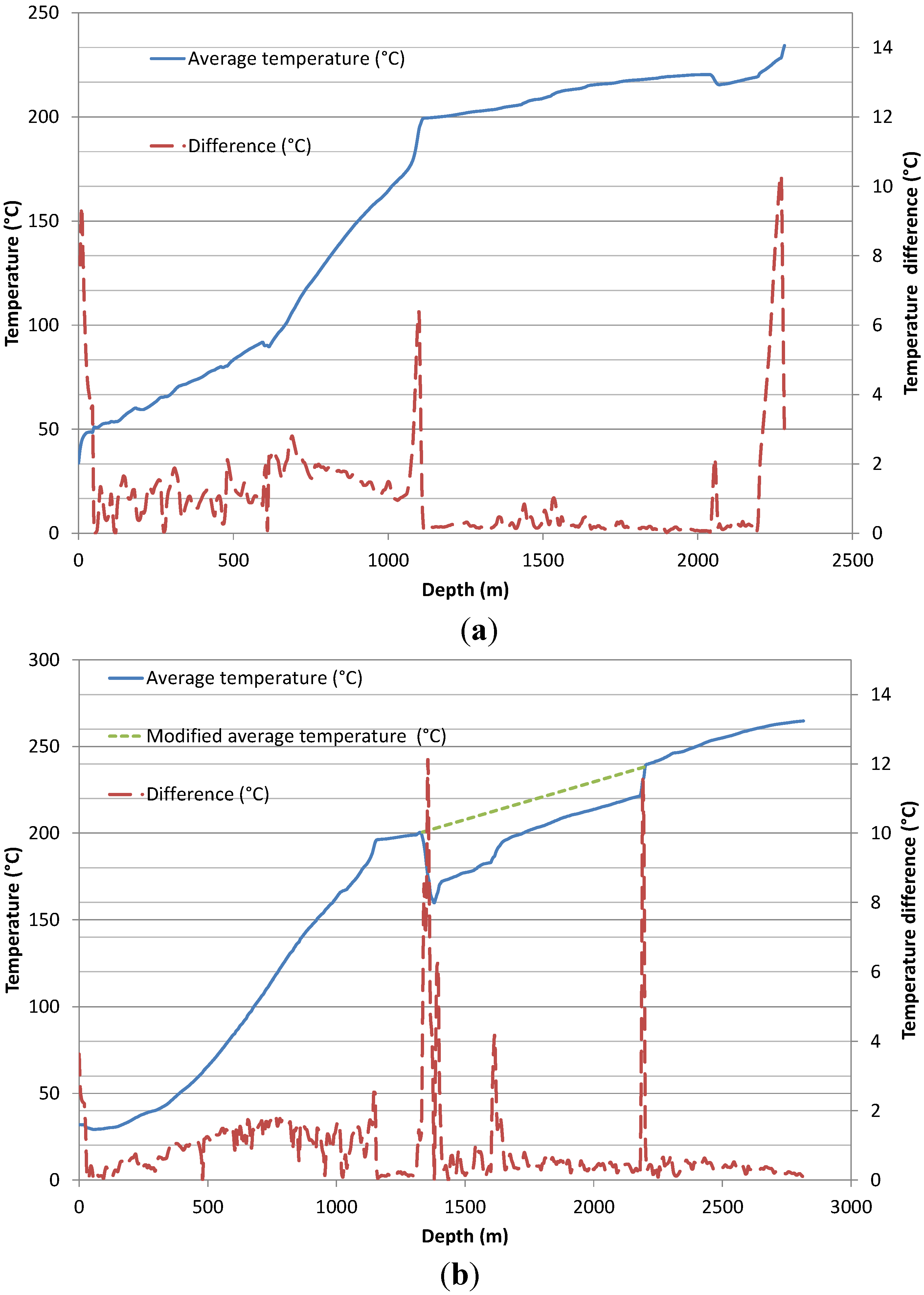
There is a low temperature gradient between 1150 and 2800 m of about 50 °C/km. This low gradient is consistent with a high temperature convective upflow with a heat source below 2800 m depth and is unlikely to be associated with an outflow which would be associated with a temperature inversion at depth.
Between 1105 and 1150 m, there is a rapid increase from 50 to 190 °C/km in thermal gradient which indicates a switch from convective to conductive heat transfer. The rapid change in gradient indicates an impermeable barrier which impedes fluid flow across the depth at which the gradient change occurs. This impermeable barrier is consistent with the impermeable smectite clay cap observed in this depth range.
Figure 6. Plot showing variation in well temperature and variation in normalized seismic velocity anomaly (Vpn) with depth as derived from the tomographic model of Shalev et al. [13]. The Vpn values used are the average value for wells MON-1 and MON-2. (a) Values for well MON-1; (b) Values for MON-2.
Energies 07 06689 g006
Seismic velocity variation across high temperature geothermal reservoirs has been observed at several locations [23,24,25]. In most of these studies, seismic velocity inversion is performed on data sets consisting of natural seismic events. These data sets were generated by relatively small numbers of sources and receivers. It is also impossible to control source location and density. Models generated using passive seismic data therefore generally have limited resolution usually on the scale of kilometers; larger than the length scale of individual wells in the fields. This limited resolution makes detailed comparison between measured reservoir characteristics and seismic models impossible. In these studies, variations in seismic velocity are often ascribed to subsurface steam zones or highly saturated porous regions in the reservoir which would lower seismic velocity.
In some laboratory studies on reservoir rocks, the effects of the temperature of the saturating fluid and variations in porosity and clay concentration on measured seismic velocities were investigated [11,26]. These studies were limited in the spatial scale of the samples they could study and also in the timescale of the experiments which was (typically seconds to minutes). The temperature ranges were often limited as well. There were few measurements above 200 °C. Jaya et al. [26] explored variation in seismic velocity of highly porous (20%) liquid saturated samples. The results showed a significant decline in velocity as temperature increased. The results are explained in terms of a modified Gassman equation [27]. Boitnott [11] measured the seismic velocities of liquid saturated samples and used linear regression to determine the relative effects of porosity and clay concentrations. He found porosity to have the strongest effect on seismic velocity, with the concentration of illite having the second most significant effect. Seismic velocity was found to decrease with both increasing porosity and illite concentration.
Kiddle [22] performed a series of experiments on rock samples from Montserrat collected from the surface and upper 200 m. Both dry andesite and andesite breccia samples show little velocity variation with temperature, samples were heated up to 600 °C. However, velocity was found to increase significantly with pressure. Pressure was increased up to 70 MPa. A large variation in seismic velocity was measured between the andesite and andesite breccia samples. P-wave velocities of 2.5–5.5 km·s−1 were measured for solid andesite samples at room temperature and pressure whilst significantly lower values of 1.6–3.6 km·s−1 where measured for andesite breccia samples under the same conditions. This variation is reflected in the seismic velocity anomaly model shown in Figure A1. The dense andesite cores beneath the volcanic centers, particularly the Soufrière Hills and Centre hills, have high seismic velocities compared to the flanks which are composed largely of andesite breccia. Kiddle, however, does not address the significant variations in the velocities of the flank deposits.
The direct effect of temperature on seismic velocity seems to be an unlikely explanation for velocity variations observed in Montserrat as temperature increases monotonically with depth but the seismic velocity anomaly decreases at a depth of around 1750 m and a temperature of around 220 °C. Similarly, for porosity to be responsible for the observed pattern would require a steady increase in porosity to a depth of 1750 m after which porosity rapidly decreases. This again seems unlikely although Brophy et al. [8] do suggest there may be some stratigraphically controlled permeability/porosity at around 2100 m. The temperature pressure profile indicates that the reservoir fluid is in a liquid state as it does not cross the boiling point for depth curve.
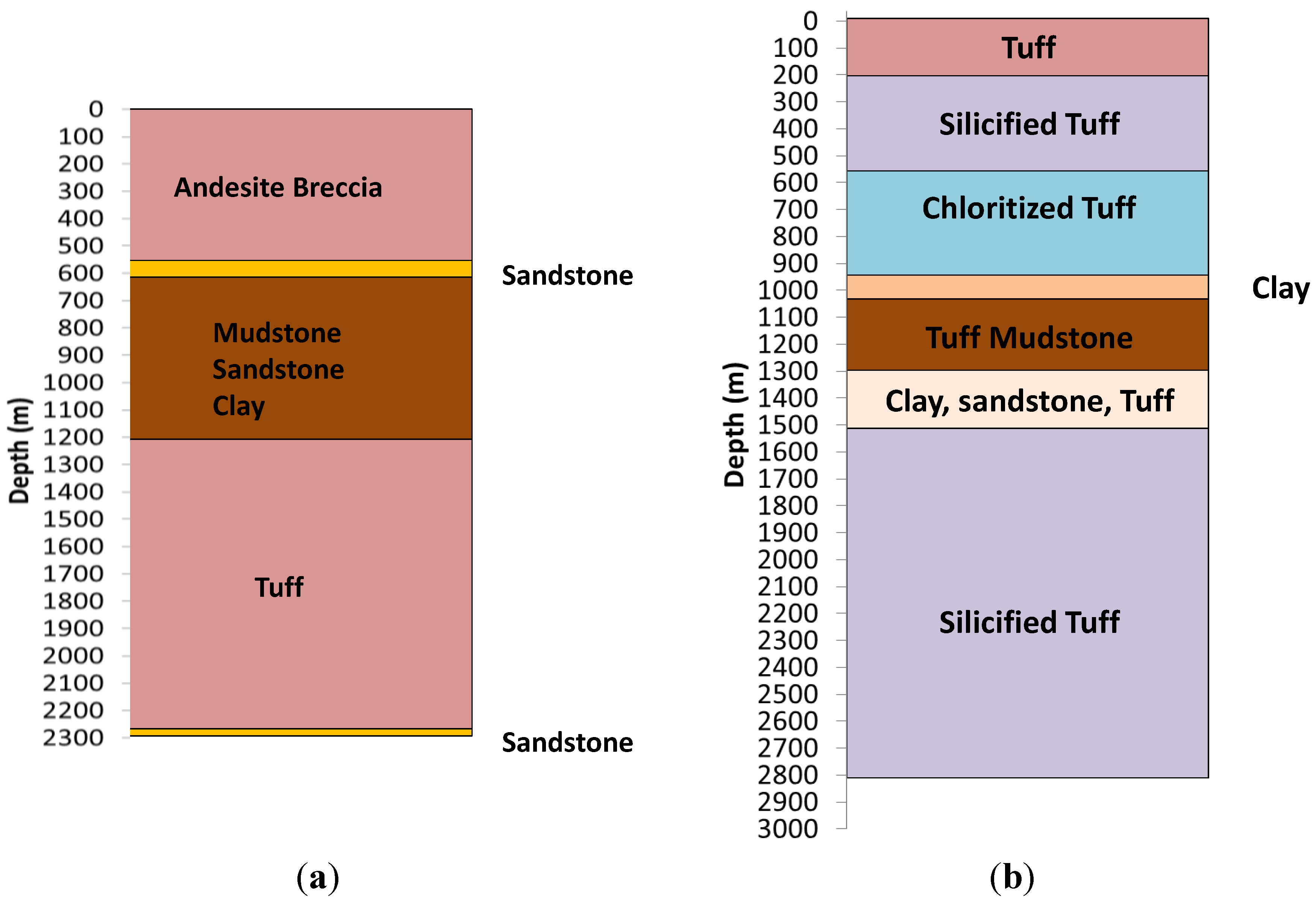
The hypothesis that hydrothermal clay alteration may be responsible for the observed velocity anomaly is feasible since cutting logs show smectite clay alteration in the 600–1200 m depth range. In assessing the hydrogeology of Montserrat, Geotermica Italiana [4] outlined the likely effects of hydrothermal alteration on reservoir rocks on the island and its effect on the mechanical properties of the rock. The effects of hydrothermal alteration at the water–rock interfaces give a possible explanation for the observed variations in seismic velocity.
At intermediate temperatures between 90 and 130 °C superficial alteration processes (weathering) are greatly enhanced and smectite clay is formed. Rather than being removed via erosional processes as it would be at the surface this swelling clay accumulates along preferential flow pathways reducing porosity to form an impermeable barrier. At the higher temperatures of 130–200 °C, phyllic alteration occurs with the formation of first interlayered illite-smectite and finally illite at temperatures above 200 °C. This process causes the rock to become more plastic [4].
Between 200 and 300 °C, we have propylitic alteration in which minerals such as quartz, epidote and adularia are formed; as the proportion of these framework silicates increases the reservoir rocks become more rigid and crystalline. Whilst permeability in these rocks can be reduced by deposition of silica, this can be easily reversed by tectonic activity.
This sequence of alteration gives a possible explanation for the observed velocity anomaly. Formation of phylosillicate clays, in particular illite, acts to plasticise the rock and reduce seismic velocity (increase seismic velocity anomaly) up to a temperature of around 200 °C; above this temperature propylitic alteration progressively increases the rigidity of the rocks causing an increase in seismic velocity (decrease in seismic velocity anomaly). This pattern of hydrothermal alteration represents the commonly observed pattern of alteration observed in high-temperature geothermal systems hosted in andesite rocks [28]. Similar patterns of hydrothermal alteration are reported in the geologically similar neighbouring island of Guadeloupe [29,30]. This pattern of alteration is also used to interpret the resistivity anomalies associated with high temperature geothermal systems [15,31]. Further detailed studies of the mineralogy of existing samples along with samples, including possible core, from future wells in Montserrat is required to verify the petrology.
One of the difficulties in trying to infer reservoir seismic properties from the laboratory results is that separate phenomena are likely convolved. Variations in fluid temperature change its contribution to the P-wave velocity. At the same time, the properties of the rock matrix vary with temperature as a function of changes in the equilibrium assemblage of hydrothermal minerals. Experiments of Jaya et al. [26] take place on much too short a timescale for equilibrium alteration to occur and the experiments of Boitnott [11] which investigate the effect of variations in porosity and variations in the concentration of hydrothermal clays all take place at a single temperature.
Experiments conducted by Kiddle [22] which investigate the effect of temperature and pressure on rock from Montserrat were conducted on dry rock samples from the surface and shallow subsurface and are not representative of saturated altered reservoir rocks. Experiments on saturated samples were also conducted but these were performed at room temperature and pressure. These experiments showed little effect of temperature on P-wave velocity but a large velocity variation was measured between andesite and andesite breccia with P-wave velocities for breccia being significantly lower. The high velocity zones seen in the velocity perturbation maps in the appendix is clearly related to the dense andesite cores associated with the volcanic centers [13,22]. However, there is a significant variation in P-wave velocity in the flank deposits. We suggest that the flank deposits with the anomalously low velocities, particularly the anomaly in the southwest of the island which is co-located with a verified geothermal system, are associated with hydrothermal alteration.
The lateral variation in the P-wave velocity of the flank deposits coupled with the fact the seismic velocity anomalies peak at a depth of 1750 m or so (within the zone of potential phyllic alteration within the reservoir) rather than being anomalous from the surface to depth supports the hypothesis that the velocity variations are dominated by changes in the hydrothermal mineral assemblage.

3.2. Correlation between Seismic Anomaly and Temperature

Figure 7 suggests, as was postulated in Ryan et al. [9], that there is a robust correlation between reservoir temperature and seismic velocity. To test this hypothesis, we recast the data to explore the correlation between the two. For this analysis, we combine the data from wells MON-1 and MON-2 to obtain the maximum number of data points under the assumption that the wells, which are approximately 500 m apart, sample similar regions of the reservoir. This assumption is supported by the similarity between the temperature profiles and the normalized seismic velocity anomalies for both wells. The value of the percentage P-wave velocity perturbation is multiplied by −1 to create positive values for the seismic velocity anomaly.
Figure 7. Correlation plot for normalised seismic velocity anomaly (Vpn) and reservoir temperature. Data for wells MON-1 and MON-2 are combined. Three different correlation regimes (R1a, R1b and R2) are suggested by the data. One point has been rejected as an outlier. This point which relates to the bottom of well MON-1 is thought to be slightly distorted.
Energies 07 06689 g007
To produce this correlation plot, the resolution of the temperature data was reduced to match the resolution of the resampled seismic velocity model. The temperatures were averaged over 250 m intervals. The data suggest three dominant regimes (Vpn refers to normalised seismic velocity anomaly and T refers to reservoir temperature in °C):
(1)
A slow increase in seismic velocity anomaly with temperature between 29 and 192 °C characterized by the following Equation (2) which fits the data with an R2 value of 0.95
V p n = 0.003 T 0.08
(2)
A rapid increase in seismic velocity anomaly with temperature between 192 and 219 °C characterized by Equation (3) which fits the data with an R2 value of 0.90
V p n = 0.021 T 3.6
(3)
A rapid decrease in seismic velocity anomaly with temperature between 219 and 263 °C characterized by Equation (4) which fits the data with an R2 value of 0.96
V p n = 0.015 T + 4.4
The decision to parameterize the correlation data in the way described above is purely empirical and is strictly only valid for the local area and for the specific set of tomographic inversion parameters used. The linear fits were chosen for their simplicity and because they provide a good fit to the data. The correlation could have been parameterized using different functions.
The observed correlation is between temperature data obtained from well logs and the magnitude of Vpn obtained from inversion of active seismic data [13]. As with all geophysical inversions, the inverse model here is non-unique [32] as discussed in Section 2.2. The exact form of the inverse model is dependent on the damping parameters used to stabilize the inversion. The values were chosen to maximize the structural information contained within the seismic data whilst minimizing the effects of errors inherent in the data which make it difficult to obtain a solution to the ill-conditioned inverse problem [32].
The correlations between Vpn and temperature we obtain are not solely a function of subsurface geology but also depend on the inversion parameters chosen. A related consequence of the inversion process is the tendency for geological anomalies to be “smeared out” which limits the ability of the inversion to resolve small anomalies. Checkerboard test results shown in the appendix show that the resolving power of the data remains good down to a depth of 3 km. Structures at the sub-kilometer scale are resolvable at this depth in the region of the geothermal reservoir. The checkerboard test data (appendix) also illustrates how the initial model is “distorted” by the inversion process. The intensity of the anomaly decreases and the anomaly spreads out in space. Whilst the intensity of the anomaly varies, its general shape, although blurred tends to be stable. For this reason, we use the normalised seismic velocity anomaly in our analysis to reduce the effect of the particular choice of damping parameters on the magnitude of velocity anomaly.
Our favoured interpretation of the variation in seismic velocity with temperature is that it is related to the assemblage of hydrothermal minerals at different temperatures with clays being formed between 70 and 220 °C which progressively plasticise the rock matrix and reduce bulk and shear moduli of the rock and thus reduce P-wave velocity. Above 220 °C propyllitic alteration occurs which increases the proportion of framework silicate minerals such as quartz, epidote and adularia. This change increases the rigidity of the rock and increases the elastic moduli, again increasing P-wave velocity.
Alternate explanations for the observed low velocity anomalies such as variations in lithology, porosity, fluid saturation and cementation are also possible. None of these alternatives, however, directly explain the variation of the anomaly with depth, in particular why it peaks at a depth of around 1750 m in the region of the two wells. Alternate explanations cannot be totally rejected without further investigation, particularly of the cuttings from the existing wells. Core from future wells would be particularly valuable in future studies.

3.3. Creating a 3-D Temperature Model

Having determined that a correlation between seismic velocity anomaly and temperature exists, the next step is to use this correlation to estimate the subsurface temperature field from the seismic tomographic data. Knowing how subsurface temperatures vary in 3D will shed light on subsurface fluid flow pathways that would be of interest in geothermal energy exploitation.
Assuming our hypothesis explaining the cause of seismic velocity variation is sufficiently correct, it would be straightforward to convert the seismic anomaly data to temperature estimates if they were uniquely known. As discussed in Section 2.2, inversion of the seismic arrival data leads to “distortion” of the measured anomaly leading to variations in the shape and intensity of the modeled anomaly. If we consider the seismic anomaly data as being made up of a series of 1-D vertical columns through the model space the “distortion” will vary as we move from the edge of the anomaly to the center. In particular, the intensity of the anomaly will appear to decrease as it is “smeared out” at the edges. However, using the assumption that the maxima of the anomaly should be relatively undisturbed even if its absolute value varies and that the maximum is related to a unique process i.e., a change in hydrothermal mineral assemblage which occurs at a fixed temperature in this geothermal reservoir we propose using the normalised seismic velocity anomaly (Vpn) to “undistort” the seismic data in the region close to the wells.
The seismic velocity anomalies as measured at the locations of wells MON-1 and MON-2 which are 500 m apart have very similar, somewhat Gaussian, shapes and similar amplitudes (Figure 3). If we look at 1-D anomalies as we move away from the well locations to the edges of the anomaly we see that the shape of the anomaly remains similar but the amplitude decreases (Figure 8). We suggest compensating for this amplitude reduction in the region close to the wells, at which reservoir conditions are similar, by using Vpn. We deem this a logical approach because conditions are similar in the region close to the measurement point, and the seismic velocity anomaly has a similar cause and shape. We postulate that the anomaly maximum occurs at a fixed temperature and is caused by a change in the regime of hydrothermal alteration. We therefore suggest that the maximum occurs at the same temperature in locations close to the well. Although this is not a fully rigorous approach, it has the benefit of simplicity and transparency. Our assumption, that nearby regions are similar, should be most robust closest to the zone where temperatures were measured and becomes less certain with distance from that location.
Figure 8. Variation in seismic velocity anomaly as one moves from south to north near the location of well MON-1.The graphs relate to vertical columns through the seismic tomography perturbation model going from 5000 to 9500 m·N at 6000 m·E. Each block in the resampled model domain is a cube with side 250 m. The horizontal axis indicates the magnitude of the anomaly in %. Note also how the magnitude of the anomaly increases from the southern edge to a maximum and then decreases again.
Energies 07 06689 g008
Figure 8 shows the variation in the seismic anomaly from the tomographic model going from south to north near well MON-1. This line correlates most closely to the N-S cross-section at 6250 m·E through the estimated temperature model in Figure 9. Figure 3 shows the bell-shaped anomaly seen in the tomographic model in the vicinity of the wells. The peak of this curve is associated in our interpretative framework with a change in hydrothermal mineral assemblage above 220 °C which causes an increase in the rigidity of the rock. An interesting feature of Figure 8 is that we can see the peak of the curve indicating the change in hydrothermal mineral assemblage shallowing from south to north from about 2000 m depth to just under 1500 m. This shallowing is reflected in the estimated temperature model of Figure 9 at 6250 m·E. Figure 9 shows a shallowing of the high temperature region of the model at around 7500 m·N.
To complete this analysis efficiently we created a MATLABTM (Mathworks, Natick, MA, USA) script to automatically analyse the seismic anomaly model. The steps carried out by the script are outlined below:
(1)
Create a master anomaly by averaging the anomalies at MON-1 and MON-2. Normalise this master anomaly.
(2)
Use the master anomaly data and the averaged well temperature data to create three linear correlations between Vpn and temperature as described in Section 3.1.
(3)
Loop over each vertical 1-D column in the seismic anomaly model volume.
(4)
For each column, the anomaly is analysed to determine its similarity to the master anomaly’s roughly Gaussian shape. This is accomplished using a weighted least squares algorithm to fit an offset Gaussian function to the anomaly (Appendix).
(5)
RMS (Root Mean Square) value of the residuals between the best-fit Gaussian function and the seismic anomaly data is determined for each column of the seismic tomography model. If the RMS error is below 1/8th of the maximum value of the anomaly this is taken as a necessary but insufficient condition for similarity to the master anomaly. 
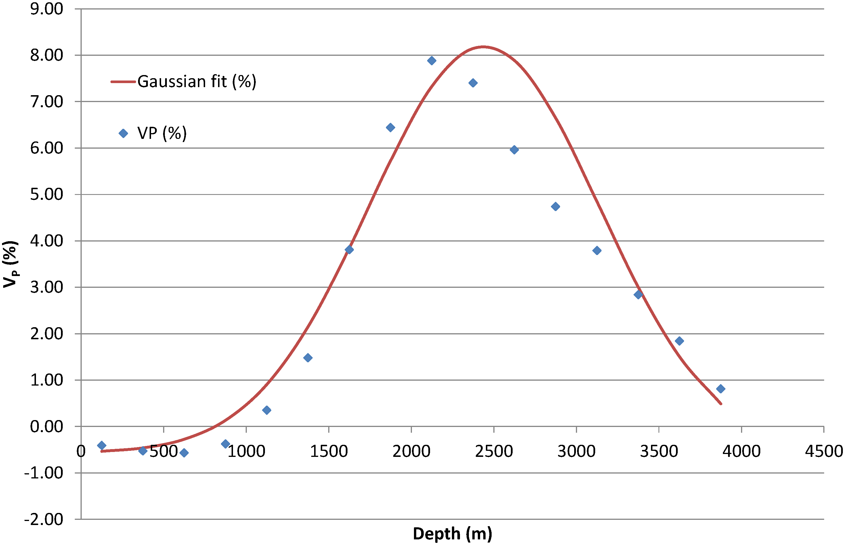
Figure 10 shows the fit of seismic anomaly data to an offset Gaussian. A perfect fit is not necessary. The purpose of the fitting is simply to gauge general similarity of shape and to estimate the amplitude of the anomaly.
(6)
If the amplitude of the seismic velocity anomaly is greater than 4% as well as having an acceptable RMS error the anomaly is deemed similar.
(7)
All “similar” anomalies are “undistorted” by normalising them to vary between 0 and 1.
(8)
The three correlations functions are used to derive temperature estimates from the “undistorted” anomaly. Care is taken to break each vertical anomaly into regions so that the region in which Vpn increases with temperature is not confused with regions in which Vpn decreases with temperature (see Figure 7).
Figure 9, Figure 11 and Figure 12 show the results of the temperature estimation algorithm. Although the results of the estimation are, according to our theoretical framework, most justifiable at the areas closest to the wells the algorithm was allowed to operate over the entire seismic anomaly model domain. Results in regions far from the wells must be looked at skeptically.
Looking at the seismic velocity perturbation model (Figure A1) we can see that temperature estimates have been made in the areas corresponding to the three regions in which there are slow seismic anomalies in the northwest, northeast and in the region of interest which is known to host a geothermal system, the southwest. The regions to the northwest and southwest cannot be interpreted with any degree of confidence since they are far from the wells that provide the correlating data. However, the analysis shows that the seismic anomalies in these three regions are similar to each other in the details of their structure.
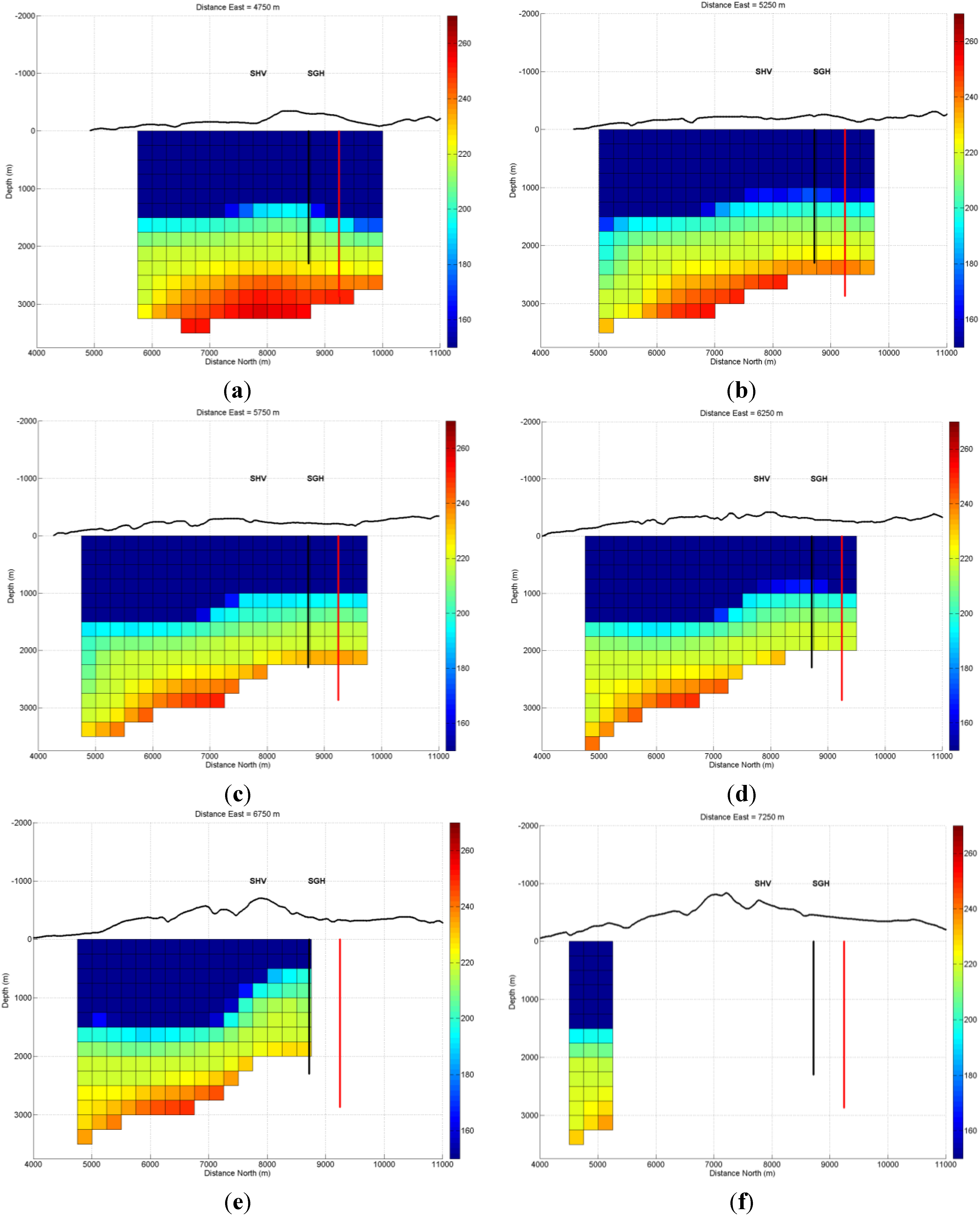
Figure 9. (af) N-S Cross-sections through the southwestern region of the temperature model estimated from the seismic velocity anomaly data. This region corresponds to seismic anomaly associated with the known geothermal system. Black line indicates the track of well MON-1 and the red line indicates the track of well MON-2. SHV (Soufrière Hills Volcano); SGH (St. George’s Hill). The colour scale indicates temperature in degrees Celsius.
Energies 07 06689 g009
Figure 10. Fit of seismic anomaly data to an offset Gaussian function. The equation constants are Δ = −0.57, k = 8.76, μ =10.26, σ = 3.95, the rms error is 0.80 (see appendix for details). A perfect fit is not necessary. The purpose of the fitting is simply to gauge general similarity of shape and to estimate the amplitude of the anomaly. This anomaly was at location 4500 m·E and 8750 m·N in the model.
Energies 07 06689 g010
The method described in this study presents the possibility of a method for estimating subsurface temperatures in a geothermal system with unprecedented resolution. Such a method would be of great use in geothermal exploration and well targeting. The interpretation framework described here requires further work to verify its validity but if it proves to be valid it would deliver another interpretation framework similar to the interpretation scheme used in interpreting resistivity anomalies in high temperature reservoirs [33]. The areas of the model domain where no temperature estimates were made do not necessarily indicate low temperature. It simply means that the form of the seismic anomaly in these regions was dissimilar to that of the master anomaly and no interpretation was made.
Focusing on the southwest anomaly we see that the estimation algorithm makes testable predictions about the geothermal system. The model indicates that the regions of shallowest high temperature occur beneath St. George’s Hill. This is consistent with an upflow in this area. The zone of high shallow temperatures can be seen particularly well in Figure 11 at the 1500 m depth. The shallowing of the high temperatures beneath St. George’s Hill is seen clearly in Figure 9 in the 6250 m east cross-section.
This finding which indicates the existence of a geothermal system with an upflow beneath St. George’s Hill away from the Soufrière Hills volcano is supported by earthquake data and resistivity data described in Ryan et al. [9] and is consistent with early results from the well logging.
The temperature anomalies indicated to the NW and NE and seen in Figure 11h are not corroborated by any evidence of active geothermal systems in these areas. However, no extensive studies have been carried out in these areas to date. A possible explanation for these zones is that they are related to zones of relict hydrothermal alteration which has modified the seismic velocities but is no longer related to a real temperature anomaly. This illustrates the constant necessity for multiple sources of information when interpreting geophysical data.
Figure 11. (ag) Planar views through the SW region of the temperature model estimated from the seismic velocity anomaly data. This region corresponds to the seismic anomaly associated with the known geothermal system; (h) Planar view through the entire temperature model at a depth of 2000 m. Apparent temperature anomalies to the NW and NE may only be indicative of relict hydrothermal alteration in these locations or some other process altogether. The NW trending black line indicates a zone of structural weakness identified by Wadge and Isaacs [34]. The NE trending black line indicates a fault plane identified from earthquake hypocenters beneath St. George’s Hill [9]. The magenta dots relate to the locations of wells MON-1 and MON-2. The cyan dot relates to the location of the alkali-chloride hot spring at Hot Water pond. GBH (Garibaldi Hill); SGH (St. George’s Hill); GM (Gage’s Mountain); CP (Chances Peak); SHV (Soufrière Hills Volcano); RM (Roche’s Mountain); SSH (South Soufrière Hills); RE (Roche’s Estate); CH (center Hills); SH (Silver Hills). The colour scale indicates temperature in degrees Celsius.
Energies 07 06689 g011
Figure 12. (af) E-W Cross-sections through the southwestern portion of the temperature model estimated from the seismic velocity anomaly data. This region corresponds to seismic anomaly associated with the known geothermal system. Black line indicates the track of well MON-1 and the red line indicates the track of well MON-2. SGH (St. George’s Hill). The colour scale indicates temperature in degrees Celsius.
Energies 07 06689 g012

4. Conclusions and Further Work

The main conclusion of this study is that there is persuasive evidence to suggest that seismic velocities in a high temperature geothermal reservoir are strongly influenced by temperature dependent hydrothermal mineral assemblages. We suggest that this influence may allow seismic velocity anomalies to be used to estimate reservoir temperatures. Further work, however, is required to fully reject alternate possibilities.
Sub-surface temperature estimation suggests the existence of an upflow zone beneath St. George’s Hill in the geothermal system in the southwest of Montserrat. Estimated “temperature anomalies” in the northwest and northeast of the island are possibly due to relict hydrothermal alteration related to extinct geothermal systems.
The current interpretation scheme for the seismic velocity anomaly data is based on a pattern of hydrothermal alteration commonly seen in high temperature geothermal systems [15]. However, further work on the petrology of samples from Montserrat’s geothermal wells is required to determine whether the details of hydrothermal alteration in this case are consistent with the seismic interpretation.
The methods used to correlate temperature log data to the seismic anomaly data, and particularly to “undistort” the seismic anomaly data, are empirical and crude. A more rigorous approach should be sought in future work.
In a similar vein, it may be possible to obtain a more theoretically robust method for correlating seismic anomalies to hydrothermal alteration by using Gassman’s equation [27] in tandem with experimental results on the physical properties of hydrothermally altered rocks.

Acknowledgments

We thank the government of Montserrat for permission to publish the results of this study. We are also very grateful to those who supported the SEA-CALIPSO study including NSF, NERC, Discovery Channel, British Geological Survey, Foreign and Commonwealth office, PASSCAL Instrument centre and the Montserrat Volcano Observatory. Although originally for another purpose this data set has proved to be a unique and valuable addition to research in geothermal exploration; the kind of happy accident which often occurs in science. We are also grateful to Pat Browne and Bridget Lynne for many informative discussions on hydrothermal alteration in geothermal systems. The Institute of Earth Science and Engineering is also acknowledged for providing us with time to work on this study. We gratefully acknowledge the three anonymous reviewers whose thoughtful work helped to greatly improve the clarity of this manuscript.

Author Contributions

Graham Ryan formulated the project’s original concept and wrote the manuscript. He is also responsible for developing the algorithms used to analyse the well temperature log and tomographic model data, and wrote the scripts used to generate the 3-D temperature model. Eylon Shalev was responsible for creating the Vp tomographic model along with data for the Vp perturbation model, ray hit and checkerboard test plots. He also reviewed the manuscript.

Appendix

A.1. Seismic Tomography

Figure A1. P-wave tomography results from Shalev et al. [13] displayed as perturbation from the average velocity at each depth. Blue represents faster velocities and red represents slower velocities. (a) map view slice through the target volume at 2000 m depth; (b) E-W cross-sections through target volume at 8750 m north; and (c) 6750 m north; (d) N-S cross-section through target volume at 5250 m east; and (e) 6250 m east. The NW trending black line indicates a zone of structural weakness identified by Wadge and Isaacs [34]. The NE trending black line indicates a fault plane identified from earthquake hypocenters beneath St. George’s Hill [9]. The magenta dots relate to the locations of wells MON-1 and MON-2. The cyan dot relates to the location of the alkali-chloride hot spring at Hot Water pond. GBH (Garibaldi Hill); SGH (St. George’s Hill); GM (Gage’s Mountain); CP (Chances Peak); SHV (Soufrière Hills Volcano); RM (Roche’s Mountain); SSH (South Soufrière Hills); RE (Roche’s Estate); CH (center Hills); SH (Silver Hills). The colour scale indicates % velocity perturbation.
Energies 07 06689 g013
Figure A2. Number of observations used in the seismic tomography inversion shown for each on-shore seismometer. Red dots indicate Reftek seismometers. Green dots indicate Texan miniature seismic recorders and blue dots indicate seismometers which are part of the permanent monitoring network of the Montserrat Volcano Observatory.
Energies 07 06689 g014
Figure A3. Location of seismometers (red triangles) used in this study located on-island and off-shore. The green line indicates the track of the vessel towing the air-gun seismic source. The green and purple dots mark the positions of wells MON-1 and MON-2, respectively. The blue outline surrounding the island indicates the extent of a shallow submarine platform.
Energies 07 06689 g015
Figure A4. Ray hit counts for the tomographic inversion domain including. The panels show the number of rays that pass through 250 m × 250 m × 250 m boxes at (a) 0 m; (b) 500 m; (c) 1000 m; (d) 2000 m and (e) 3000 m depth. Only the center portion of the tomography box is plotted, with the outline of Montserrat in black. Colors indicate the log10 of the number of rays that track through each box.
Energies 07 06689 g016
Figure A5. Checkerboard test results for anomalies at (b) 0 km; (c) 0.5 km; (d) 1 km; (e) 2 km; (f) 3 km and (g) 4 km depths; (a) is the source pattern for the checkerboard test (shown at 3 km depth). The x and y-axes indicate distance in km east and north respectively. The colour scale indicates percentage velocity perturbation. Synthetic noise with a zero-mean Gaussian distribution and 0.02 s standard deviation was added to the travel-time data. Note the variation in the amplitudes of anomalies.
Energies 07 06689 g017

A.2. Gaussian Fitting Algorithm

In order to determine the similarity of 1-D columns through the seismic velocity anomaly model to the seismic anomalies observed at the locations of wells MON-1 and MON-2, we exploited the similarities of the seismic anomalies as a function of depth to offset Gaussian functions following the equation:
Energies 07 06689 i001
where Vp is the magnitude of the seismic anomaly, k is a scaling factor, d is depth below sea level in meters, μ is the depth at which the peak Vp magnitude occurs, σ is the characteristic width of the Gaussian function and Δ is a scalar offset.
In order to obtain a simple linear function we assume that Δ is a known value and simply minimize the remaining Gaussian function once it has been subtracted:
Energies 07 06689 i002
To obtain a linear equation, we take the natural logarithm of both sides of the equation to obtain a polynomial in d:
Energies 07 06689 i003
Treating the variables d and d2 as linear variables, we can do a simple weighted least squares parameter estimation using Equation (A4).
In order to bias the fitting algorithm to fit the peaks of the anomalies at the expense of the tails, we employed a weighted least squares algorithm. In which the errors varied monotonically from 1/10th to 1/100th of the average value of lnVp from the initial low value to the peak value of the anomaly and then back to 1/10th. This error information is captured in the diagonal matrix C where the leading diagonal contains the squared reciprocals of the corresponding error values:
Xw⟩ = [ATCA]ATCb
where ⟨Xw⟩ is the vector of linear best-fit coefficients of Equation (A3), A is the matrix of linear variables in Equation (A3) and b is the vector of lnVp values. The parameters μ, σ and k can be recovered from simple rearrangement of the elements of ⟨Xw⟩. To generate the best-fit parameters from data from a 1-D seismic anomaly, we simply use Equation (A4) using the values of ln Vp, d and d2. A description of weighted least squares estimation can be found in any book on elementary linear algebra, e.g., [35].
The RMS error of the fit of the data to the Gaussian model is obtained using the Equation (A5):
Energies 07 06689 i004
where Vpmeas is the value from the seismic velocity anomaly model and Vpfit is the estimate derived from the best fit model. n is the number of data points in the 1-D column.

Conflicts of Interest

The authors declare no conflict of interest.

References

  1. Wadge, G.; Voight, B.; Sparks, R.S.J.; Cole, P.D.; Loughlin, S.C.; Robertson, R.E.A. An overview of the eruption of Soufrière Hills Volcano, Montserrat from 2000 to 2010. Geol. Soc. Lond. Mem. 2014, 39, 1–40. [Google Scholar] [CrossRef]
  2. PKF. Feasibility Study into Montserrat Geothermal Energy Final Report; PKF Accountants & Business Advisers: London, UK, 2012; p. 56. [Google Scholar]
  3. Wright, E.P.; Murray, K.H.; Bath, A.H. Draft Report on Geothermal Investigations in Montserrat; WD/OS/76/012; Institute of Geological Sciences, Hydrogeological Department: London, UK, 1976; p. 62. [Google Scholar]
  4. Geotermica Italiana. Exploration for Geothermal Resources in the Eastern Caribbean; TCDCON15/90-RLA/87/037; United Nations Department of Technical Cooperation for Development: Pisa, Italy, 1991. [Google Scholar]
  5. Principe, C. Geothermal Potential in Montserat: Scoping Survey Report; Instituto di Geoscienze e Georisorse, CNR: Pisa, Italy, 2008; p. 24. [Google Scholar]
  6. EGS Inc. Final Report Geothermal Exploration in Montserrat, Caribbean; EGS Inc.: Santa Rosa, CA, USA, 2010; p. 189. [Google Scholar]
  7. Younger, P.L. Reconnaissance assessment of the prospects for development of high-enthalpy geothermal energy resources, Montserrat. Q. J. Eng. Geol. Hydrogeol. 2010, 43, 11–22. [Google Scholar] [CrossRef]
  8. Brophy, P.; Poux, B.; Suemnicht, G.; Hirtz, P.; Ryan, G. Preliminary results of deep geothermal drilling and testing on the island of Montserrat. In Proceedings of the Thirty-Ninth Workshop on Geothermal Reservoir Engineering, Stanford, CA, USA, 24–26 February 2014; p. 11.
  9. Ryan, G.A.; Peacock, J.R.; Shalev, E.; Rugis, J. Montserrat geothermal system: A 3D conceptual model. Geophys. Res. Lett. 2013, 40, 2038–2043. [Google Scholar] [CrossRef]
  10. Kristinsdóttir, L.H.; Flóvenz, O.G.; Árnason, K.; Bruhn, D.; Milsch, H.; Spangenberg, E.; Kulenkampff, J. Electrical conductivity and P-wave velocity in rock samples from high-temperature Icelandic geothermal fields. Geothermics 2010, 39, 94–105. [Google Scholar] [CrossRef]
  11. Boitnott, G.N. Core Analysis for the Development and Constraint of Physical Models of Geothermal Reservoirs; DE-FG07–99ID13761; New England Research, Inc.: White River Junction, VT, USA, 2003; p. 52. [Google Scholar]
  12. Voight, B.; Sparks, R.S.J. Introduction to special section on the Eruption of Soufrière Hills Volcano, Montserrat, the CALIPSO Project, and the SEA-CALIPSO Arc-Crust Imaging Experiment. Geophys. Res. Lett. 2010, 37, 4. [Google Scholar] [CrossRef]
  13. Shalev, E.; Kenedi, C.L.; Malin, P.; Voight, V.; Miller, V.; Hidayat, D.; Sparks, R.S.J.; Minshull, T.; Paulatto, M.; Brown, L.; et al. Three-dimensional seismic velocity tomography of Montserrat from the SEA-CALIPSO offshore/onshore experiment. Geophys. Res. Lett. 2010, 37, 6. [Google Scholar] [CrossRef]
  14. Ryan, G.A.; Onacha, S.A.; Shalev, E.; Malin, P.E. Imaging the Montserrat Geothermal Prospect Using Magnetotelluric (MT) and Time Domain Electromagnetic Induction (TDEM) Measurements; 16366.00-2009.01; Institute of Earth Science and Engineering: Auckland, New Zealand, 2009; p. 77. [Google Scholar]
  15. Anderson, E.; Crosby, D.; Ussher, G. Bulls-eye—simple resistivity imaging to reliably locate the geothermal reservoir. In Proceedings of the World Geothermal Congress, Kyushu-Tohoku, Japan, 28 May–10 June 2000; pp. 909–914.
  16. EGS Inc. Well Completion Report MON-1 and MON-2; Government of Montserrat, Public Works Department: Woodlands, Montserrat, 2014; p. 310.
  17. Gunderson, R.; Cumming, W.; Astra, D.; Harvey, C. Analysis of smectite clays in geothermal drill cuttings by the methylene blue method: For well site geothermometry and resistivity sounding correlation. In Proceedings of the World Geothermal Congress, Kyushu-Tohoku, Japan, 28 May–10 June 2000; pp. 1175–1181.
  18. Shalev, E.; Lees, J.M. Cubic B-splines tomography at Loma Prieta. Bull. Seismol. Soc. Am. 1998, 88, 256–269. [Google Scholar]
  19. Paige, C.C.; Saunders, M.A. LSQR: An algorithm for sparse linear equations and sparse least squares. Trans. Math. Softw. 1982, 8, 43–71. [Google Scholar] [CrossRef]
  20. Reidel, D.; Holland, D. Seismic wave propagation and seismic tomography. In Seismic Tomography; Nolet, G., Ed.; Reidel Publishing Company: Dordrecht, The Netherlands, 1987; pp. 1–47. [Google Scholar]
  21. Press, W.H.; Teukolsky, S.A.; Vetterling, W.T.; Flannery, B.P. Numerical Recipes in C: The Art of Scientific Computing, 2nd ed.; Cambridge University Press: Cambridge, UK, 1992. [Google Scholar]
  22. Kiddle, E.J. The Structure of the Crust and Magmatic System at Montserrat, Lesser Antilles. Ph.D. Thesis, University of Bristol, Bristol, UK, 2011. [Google Scholar]
  23. Hauksson, E.; Unruh, J.R. Interaction of shallow and deep geothermal reservoirs at Coso, Eastern California, as inferred from 3-D seismic velocity models and seismicity. Geotherm. Resour. Counc. Trans. 2004, 28, 659–662. [Google Scholar]
  24. Nakajima, J.; Hasegawa, A. Tomographic imaging of seismic velocity structure in and around the Onikobe volcanic area, northeastern Japan: Implications for fluid distribution. J. Volcanol. Geotherm. Res. 2003, 127, 1–18. [Google Scholar] [CrossRef]
  25. Gunasekera, R.C.; Foulger, G.R.; Julian, B.R. Reservoir depletion at the Geysers geothermal area, California, shown by four-dimensional seismic tomography. J. Geophys. Res. B Solid Earth 2003, 108, 11. [Google Scholar] [CrossRef]
  26. Jaya, M.S.; Shapiro, S.A.; Kristinsdóttir, L.H.; Bruhn, D.; Milsch, H.; Spangenberg, E. Temperature dependence of seismic properties in geothermal rocks at reservoir conditions. Geothermics 2010, 39, 115–123. [Google Scholar] [CrossRef]
  27. Avseth, P.; Mukerji, T.; Mavko, G. Quantitative Seismic Interpretation: Applying Rock Physics Tools to Reduce Interpretation Risk; Cambridge University Press: Cambridge, UK, 2010; p. 371. [Google Scholar]
  28. Inoue, A. Formation of clay minerals in hydrothermal environments. In Origin and Mineralogy of Clays; Velde, B., Ed.; Springer: Berlin, Germany, 1995; pp. 268–329. [Google Scholar]
  29. Bouchot, V.; Sanjuan, B.; Traineau, H.; Guillou-Frottier, L.; Thinon, I.; Baltassat, J.M.; Fabriol, H.; Bourgeois, B.; Lasne, E. Assessment of the bouillante geothermal field (Guadeloupe, French West Indies): Toward a conceptual model of the high temperature geothermal system. In Proceedings of the World Geothermal Congress, Bali, Indonesia, 25–29 April 2010; p. 8.
  30. Mas, A.; Guisseau, D.; Patrier Mas, P.; Beaufort, D.; Genter, A.; Sanjuan, B.; Girard, J.P. Clay minerals related to the hydrothermal activity of the Bouillante geothermal field (Guadeloupe). J. Volcanol. Geotherm. Res. 2006, 158, 380–400. [Google Scholar] [CrossRef]
  31. Simmons, S.; Browne, P.R.L. Three dimensional model of the distribution of hydrothermal alteration minerals within the ohaaki-broadlands geothermal field. In Proceedings of the 12th New Zealand Geothermal Workshop, Auckland, New Zealand, 7–9 November 1990; pp. 25–30.
  32. Parker, R.L. Geophysical Inverse Theory; Princeton University Press: Princeton, NJ, USA, 1994; p. 400. [Google Scholar]
  33. Ussher, G.; Harvey, C.; Johnstone, R.; Anderson, E. Understanding the resistivities observed in geothermal systems. In Proceedings of the World Geothermal Congress, Kyushu-Tohuku, Japan, 28 May–10 June 2000; pp. 1915–1920.
  34. Wadge, G.; Isaacs, M.C. Mapping the volcanic hazards from Soufriere Hills Volcano, Montserrat, West Indies using an image processor. J. Geol. Soc. 1988, 145, 541–552. [Google Scholar] [CrossRef]
  35. Strang, G. Introduction to Linear Algebra, 4th ed.; Wellesley Cambridge Press: Wellesley, MA, USA, 2009. [Google Scholar]

