A Static Voltage Security Region for Centralized Wind Power Integration—Part II: Applications

Abstract

In Part I of this work, a static voltage security region was introduced to guarantee the safety of wind farm reactive power outputs under both base conditions and N-1 contingency. In this paper, a mathematical representation of the approximate N-1 security region has further studied to provide better coordination among wind farms and help prevent cascading tripping following a single wind farm trip. Besides, the influence of active power on the security region is studied. The proposed methods are demonstrated for N-1 contingency cases in a nine-bus system. The simulations verify that the N-1 security region is a small subset of the security region under base conditions. They also illustrate the fact that if the system is simply operated below the reactive power limits, without coordination among the wind farms, the static voltage is likely to exceed its limit. A two-step optimal adjustment strategy is introduced to shift insecure operating points into the security region under N-1 contingency. Through extensive numerical studies, the effectiveness of the proposed technique is confirmed.

1. Introduction

Centralized wind power integration in China has been beset by cascading tripping incidents involving wind farms. One of the major reasons for this is the lack of coordinated voltage/reactive power control [1–9]. A number of techniques have been investigated to maintain the voltage within a specified range and improve the system stability for a single wind farm [10–17]. However, in centralized integration of wind power, interdependency among wind farms and cascading tripping events further complicate the voltage control problem. The methods developed for a single wind farm are not applicable, and may even have an adverse effect. A static voltage security region under normal conditions and an online method for describing it were proposed in the first part of this work [1]. Furthermore, in order to guarantee that the voltage will remain within limits under both normal operating conditions and wind farm N-1 tripping conditions, N-1 security region is studied in detail in this work.

Besides, it was pointed out in [1] that cascading trips tend to happen very quickly (usually in less than 2 s), rendering an effective response virtually impossible once an incident has begun. Thus, it is much more important to establish preventive control to maintain a reasonable operating status for all the closely coupled wind farms under normal operating conditions, and also to ensure that the wind farms will still be working within acceptable voltage limitations when an N-1 contingency occurs. Note that in this work, an N-1 contingency refers to a single wind farm trip for the sake of convenience.

Therefore, for any wind farm whose reactive power output is within this security region, the corresponding voltage will be within limits. If the operating point is outside the N-1 security region, a preventive adjustment is supposed to be carried out by the automatic voltage control (AVC) system, which necessitates a set of constraints on the wind farm voltages [18–20]. The problem of how to present such voltage constraints is also considered in this paper.

However, the security region is determined with a specified active power output from the wind farms. In other words, different levels of wind power penetration create different voltage security regions, and thus it is of interest to determine how the security region varies with respect to the active power. In practice, nearly all cascading trip faults have occurred when wind power generation at the wind farms was at a high level. Hence, an analysis of the relationship between the security region and wind power penetration will be of great value.

The remainder of the paper is organized as follows: in Section 2, the security region under N-1 contingency conditions is studied, and an optimal adjustment strategy is proposed to shift insecure operating points into the security region under N-1 contingency. In Section 3, the impact of wind penetration on the security region is examined. A nine-bus system with three wind farms is studied in Section 4, and the security region under N-1 contingency is derived. Numerical results for the optimal adjustment strategy are also presented; these provide an intuitive prospective adjustable voltage range for the AVC with minimum adjustment of the wind farm reactive power outputs. Finally, observations and conclusions are stated in Section 5.

2. The N-1 Voltage Security Region and Its Application

2.1. Summary of the First Part of Work [1]

In the first part of work, the concept of voltage security region of wind farms could be expressed as a set of constraints limiting the reactive power of each wind farm to maintain its static nodal voltage in the secure range, given the active power generation of each wind farm, which was compared with a sampling-based approach and several different linear approximation techniques. The results showed that the proposed method expected to produce an approximate security region that was very close to the actual one, and could be easily represented in closed mathematical form, while greatly reducing the required computations.

At the same time, it was pointed out in the first part of this work [1] that in order to mitigate the cascading trips, the region should ensure secure operation both under normal operating conditions and N-1 contingencies. It was obvious that normal voltage security region was the basis for N-1 voltage security region to provide better coordination among wind farms and help prevent cascading tripping when a single wind farm was tripped. If an operating point was in the normal security region, but out of the N-1 region, this meant that cascading was probably triggered by the first tripping event. Thus, even if the current operating status was normal, it was not secure enough, and preventive control measures should be carried out according to the proposed N-1 voltage security region. Therefore, we put emphasis on the calculation of normal voltage security region in Part I [1].

2.2. N-1 Static Voltage Security Region

Based on the concepts introduced in [1], the static voltage security region when wind farm w is tripped is bounded by the 2m planes $L_1^{w+}$, …, $L_i^{w+}$, …, $L_m^{w+}$, $L_1^{w-}$, …, $L_i^{w-}$, …, $L_m^{w-}$, where $L_i^{w+}$ denotes the i^th plane through the near point ξ⁺ when wind farm w is tripped, and $L_i^{w-}$ denotes the i^th plane through the near point ξ⁻ when wind farm w is tripped. Therefore, the matrices ^w+ and ^w− of Equations (2) and (3) are valid, and the overall N-1 security region can be expressed in terms of 2m(m + 1), such as matrices $\underset{w=0}{\overset{m}{\text{∪}}}\{{\mathcal{A}}^{w-},{\mathcal{A}}^{w+}\}$. The matrices will vary in real time according to active wind power generation. Note that w = 0 denotes normal operating conditions.

$$\{\begin{array}{ll}{L}_i^{w+}:\hfill & \sum _{k=1}^m{\alpha }_{ik}^{w+}{Q}_k=1\hfill \\ L_i^{w-}:\hfill & \sum _{k=1}^m{\alpha }_{ik}^{w-}{Q}_k=-1\hfill \end{array}$$

(1)

Here, ${\Theta }_{{\xi }^{w+}}=\{L_1^{w+},\dots L_i^{w+},\dots ,L_m^{w+}\}$ is the set of m planes belonging to w⁺ and ${\Theta }_{{\xi }^{w-}}=\{L_1^{w-},\dots L_i^{w-},\dots ,L_m^{w-}\}$ is the set of m planes belonging to w⁻. In other words:

$${\mathcal{A}}^{w+}\left(\begin{array}{c}{Q}_1\\ ⋮\\ Q_m\end{array}\right)=\left(\begin{array}{c}1\\ ⋮\\ 1\end{array}\right)$$

(2)

$${\mathcal{A}}^{w-}\left(\begin{array}{c}{Q}_1\\ ⋮\\ Q_m\end{array}\right)=\left(\begin{array}{c}-1\\ ⋮\\ -1\end{array}\right)$$

(3)

The linear approximation method (6a) of [1] can be used to determine the center of the security region. Let $\left[{\text{η}}_{{\xi }^{-}}^w,{\text{η}}_{{\xi }^{+}}^w\right]$ be the security region when wind farm w is tripped. Then, the N-1 security region can be expressed as $\left[\underset{w=0}{\overset{m}{\langle max\rangle }}\left({\text{η}}_{{\xi }^{-}}^w\right),\underset{w=0}{\overset{m}{\langle min\rangle }}\left({\text{η}}_{{\xi }^{+}}^w\right)\right]$. If O_a is the center of the security region, it can be written as follows:

$$O_a=\left(\langle max\rangle \left(\underset{w=0}{\overset{m}{\cup }}{\text{η}}_{{\xi }^{-}}^w\right)+\langle min\rangle \left(\underset{w=0}{\overset{m}{\cup }}{\text{η}}_{{\xi }^{+}}^w\right)\right)/2$$

(4)

Here, <max/min>(a,b,c) denotes the operator that extracts a new vector from the vectors (a,b,c), such that each component of the new vector is the maximum/minimum from among the corresponding components of the original vectors. For example, <max>((3,2,1), (1,7,6), (2,5,4)) = (3,7,6).

Similarly, each N-1 contingency can also be assessed according to its area of intersection with normal conditions. The smaller this area, the more insecure the wind farm is. Three proposed assessment indices for each scenario, including both normal conditions and a contingency, are given in Equations (5)–(7), where min(a) in Equation (6) returns the minimum component of vector a. $I_{\text{t}}^w$ represents the area of the approximate security region for each scenario, while $I_{\text{u}}^w$ and $I_{\text{s}}^w$ represent the approximate areas of each N-1 contingency and normal conditions, respectively. If the index Equation (6) is negative, the voltage security region does not exist. Otherwise, the index Equation (7) lies within the interval [0, 1], and the contingency is more severe when this index is close to 0:

$$I_{\text{t}}^w={\Vert {\text{η}}_{{\xi }^{+}}^w-{\text{η}}_{{\xi }^{-}}^w\Vert }_2$$

(5)

$$I_{\text{u}}^w=min\left(\langle min\rangle \left({\text{η}}_{{\xi }^{+}}^w,{\text{η}}_{{\xi }^{+}}^0\right)-\langle max\rangle \left({\text{η}}_{{\xi }^{-}}^w,{\text{η}}_{{\xi }^{-}}^0\right)\right)$$

(6)

$$I_{\text{s}}^w=\frac{{\Vert \langle min\rangle \left({\text{η}}_{{\xi }^{+}}^w,{\text{η}}_{{\xi }^{+}}^0\right)-\langle max\rangle \left({\text{η}}_{{\xi }^{-}}^w,{\text{η}}_{{\xi }^{-}}^0\right)\Vert }_2}{{\Vert \langle min\rangle \left({\text{η}}_{{\xi }^{+}}^0,{\text{η}}_{{\xi }^{+}}^0\right)-\langle max\rangle \left({\text{η}}_{{\xi }^{-}}^0,{\text{η}}_{{\xi }^{-}}^0\right)\Vert }_2}$$

(7)

2.3. Minimum-Adjustment Correction Method

When the current operating point is in the normal security region, but not in the N-1 security region, it is desirable to shift the operating point into the N-1 security region with minimum reactive power adjustment. An optimization model is constructed to achieve this goal. If the number of wind farms is m, the optimization model can be written as:

$$\begin{array}{cc}min& \text{∑}_{i=1}^m{\left({\text{η}}_i-{\text{η}}_i^0\right)}^2\end{array}$$

(8)

$$\begin{array}{cc}s.t.& \text{η}\in \left({\mathrm{\Omega }}_{\text{VSR}}^{N-1}=\underset{i=0}{\overset{m}{\cap }}{\mathrm{\Omega }}_{\text{VSR}}^i\right)\end{array}$$

(9)

where ${\mathrm{\Omega }}_{\text{SVD}}^{N-1}$ can be further expanded as follows, using TCs:

$$\begin{array}{cc}\text{∑}_{i=1}^m{\alpha }_i^{w+}{\text{η}}_i\le 1,i=1,\dots ,m,& w=0,\dots ,m\end{array}$$

(10)

$$\begin{array}{cc}\text{∑}_{i=1}^m{\alpha }_i^{w-}{\text{η}}_i\ge -1,i=1,\dots ,m,& w=0,\dots ,m\end{array}$$

(11)

$$Q_i^l\le {\text{η}}_i\le Q_i^h,i=1,\dots ,m$$

(12)

In this optimization model, linear approximation of the security regions is employed. Note that the number of constraints increases quadratically with m.

2.4. Two-Step Optimal Adjustment Strategy

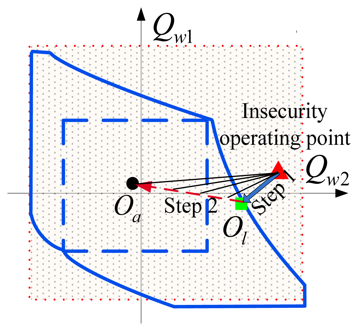
Evidently, having the operating point at the center of the N-1 security region may be the best arrangement. After an insecure operating point has been shifted as far as the security region boundary, it can be moved further into the security region, so that the greatest possible margin is maintained between it and the boundary. Figure 1 illustrates a two-step adjustment strategy that will shift an insecure operating point to somewhere inside the N-1 security region.

The first step is the minimum-adjustment correction method. Denote the result of this procedure by O_l, which is on the boundary of the security region. In the second step, this new operating point is moved further toward the center of the security region. It is intuitively clear that the nearer the point is to the center of the security region, the greater the aforementioned margin. Accordingly, the operating point is moved from O_l to O_a, and the area between the two points (defined as the “safe operating range”) remains inside the security region because of its convexity.

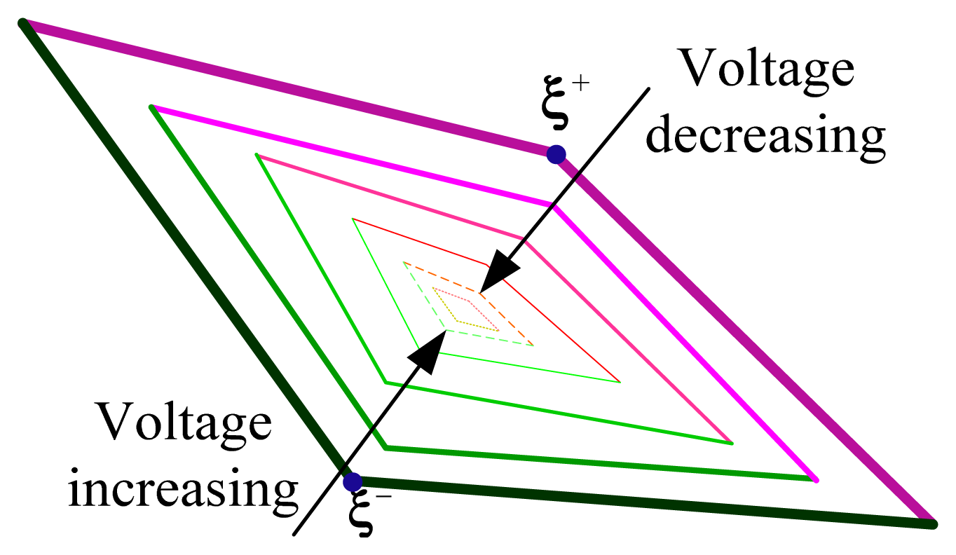
Figure 2 shows the distribution of voltage in the proposed security region. We know that equipotential lines never intersect one another. For this reason, when the operating point is moved from O_l to O_a, the corresponding voltage varies monotonically. This provides an intuitive prospective adjustable voltage range for each wind farm, given by:

$$U_{i,min}^{*}\le U_i\le U_{i,max}^{*},i=1,\dots ,m$$

(13)

where $U_{i,min}^{*}$ and $U_{i,max}^{*}$ denote the minimum and maximum voltages of wind farm i in the adjustable region. $U_{i,min}^{*}$ and $U_{i,max}^{*}$ could be used as voltage constraints in future AVC applications.

3. Impact of Wind Penetration on the Voltage Security Region

The security region is determined with a specified active power output from the wind farms. Therefore, different levels of wind power penetration create different voltage security regions. However, the initial security region is the basis of normal/N-1 security region, so we will put more emphasis on it in the following work.

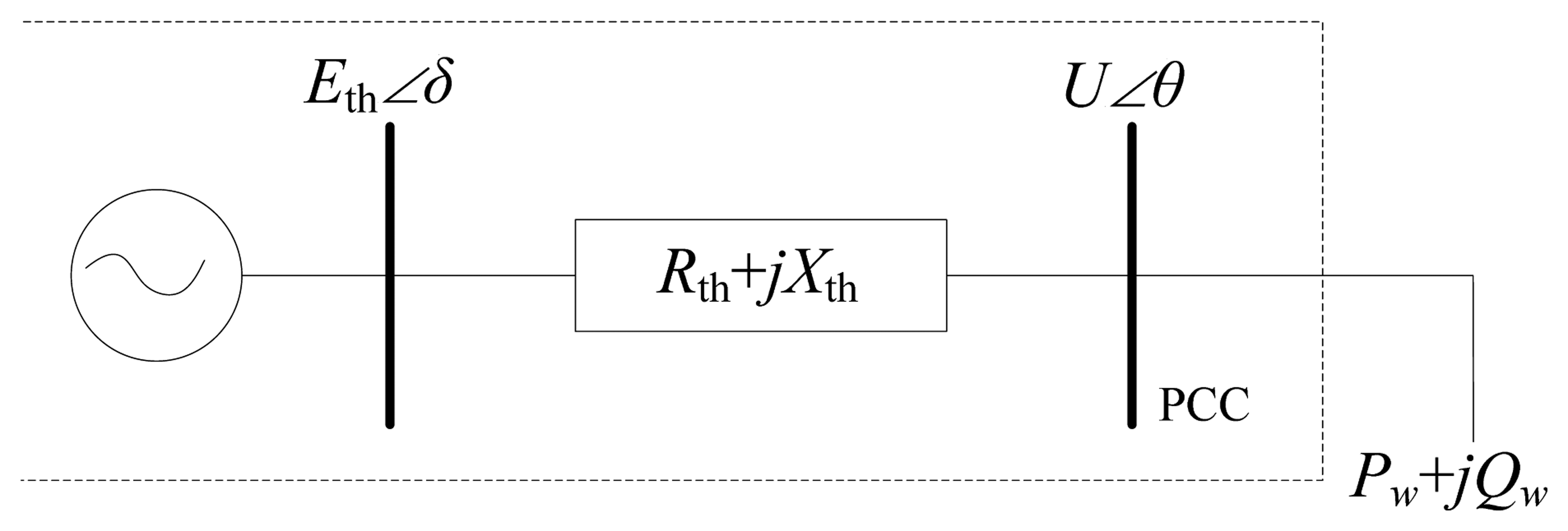
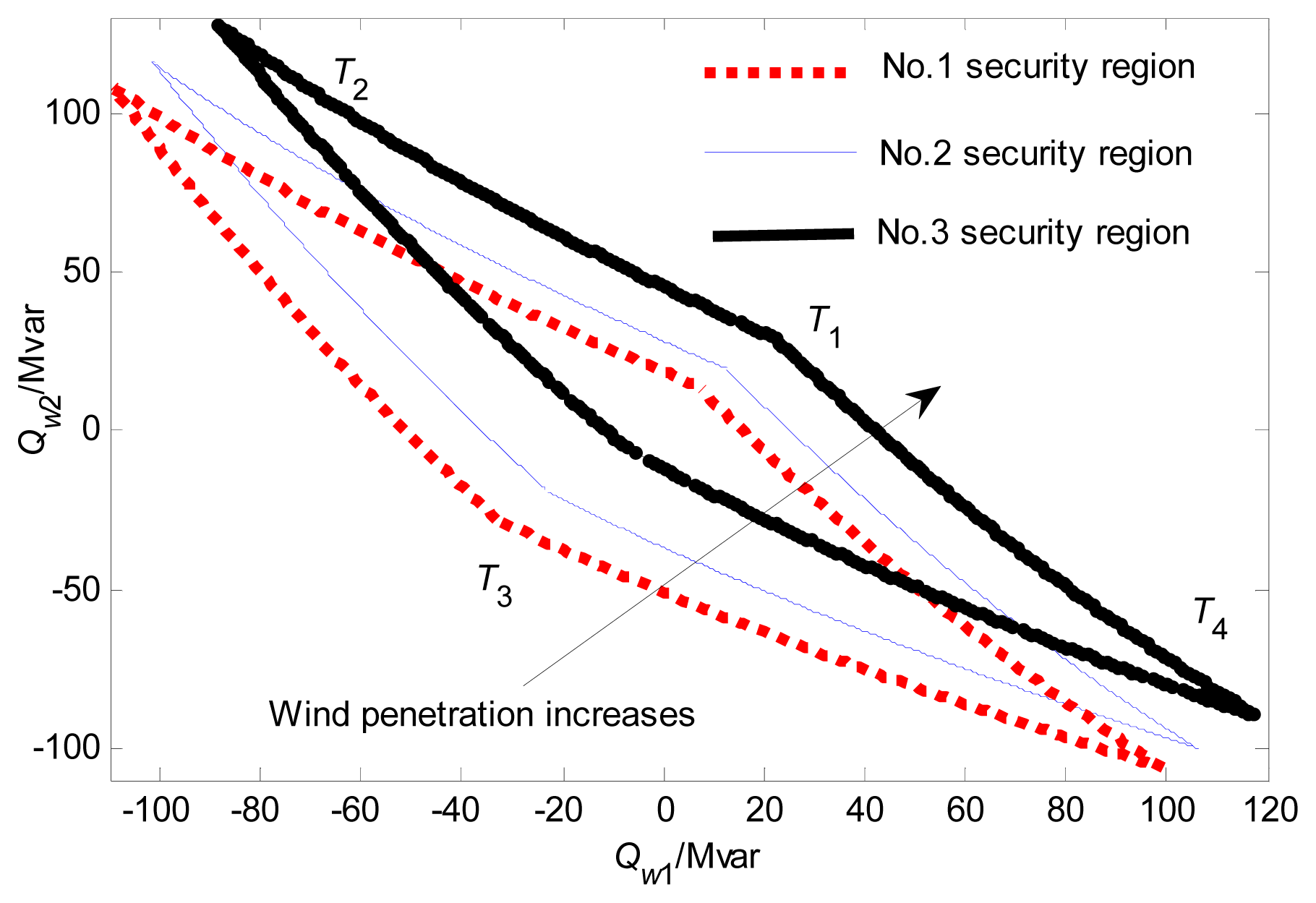
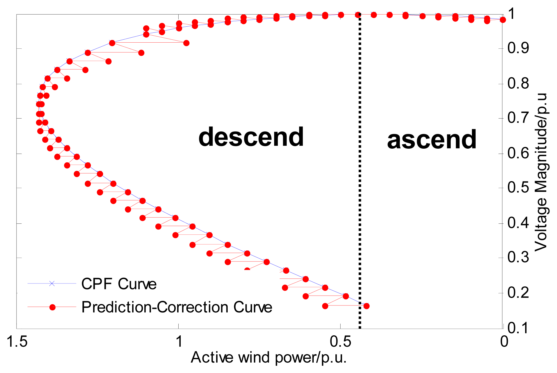
From the perspective of continuation power flow (CPF), the voltage may initially rise slightly, and then decline to the point of collapse, which is perhaps a different result from the traditional CPF for a load bus. When the nine-bus system is used as an example, the CPF is shown in Figure 3. Since a wind power injection bus can be regarded as a negative load bus, the reverse horizontal coordinate axis is used. If the Thevenin equivalent is used for the point of common coupling (PCC) (Figure 4), when the penetration is low, the impact on the system side is slight, and E_th can be regarded as a constant. Thus, an expression for the voltage drop is easily obtained from Equation (14), and indicates that the voltage rises slightly with increasing penetration. However, E_th cannot remain constant when the penetration is high, since more reactive power is consumed on X_th with the transfer of more active power, and more reactive power must be provided to keep the original voltage profile. This is why the security region moves toward the top and right with increasing wind penetration, as shown Figure 5, where initial voltage security regions are plotted for several different levels of wind penetration.

The security voltage region is obtained by the method proposed in [1] based on a modified nine-bus test system from [21].

Table 1. PCC voltage and linearity index for different wind penetration levels.

No.	Pw1 (MW)	Pw2 (MW)	PCC Voltage (p.u.)	Index La
1	60	120	1.072	2.55%
			(0.913)	(1.44%)
2	80	160	1.065	3.12%
			(0.902)	(0.22%)
3	100	200	1.055	4.09%
			(0.887)	(1.44%)

lists the PCC voltage and linearity index for different wind penetration levels. With increased wind penetration, the PCC voltage decreases due to increased reactive power losses. The linearity index L_a increases as well, indicating increased nonlinearity of the boundaries:

$$E_{\text{th}}=U-(P_w{R}_{\text{th}}+Q_w{X}_{\text{th}})/U$$

(14)

where P_w and Q_w are the active and reactive power of the wind farm; R_th and X_th are the Thevenin equivalent parameters, and E_th is the equivalent voltage.

It is also of interest to know how the area of the security region changes with increased wind penetration. To quantify this, linear approximation of the boundaries is adopted to calculate the area enclosed by Ω_S, using the following equation:

$$A_{\text{s}}=1/2\left|\stackrel{\rightharpoonup }{T_1{T}_3}\right|\left|\stackrel{\rightharpoonup }{T_2{T}_4}\right|sin\phi$$

(15)

where φ is the angle between $\stackrel{\rightharpoonup }{T_1{T}_3}$ and $\stackrel{\rightharpoonup }{T_2{T}_4}$ obtained from:

$$cos\phi =\frac{\stackrel{\rightharpoonup }{T_1{T}_3}\cdot \stackrel{\rightharpoonup }{T_2{T}_4}}{\left|\stackrel{\rightharpoonup }{T_1{T}_3}\right|\left|\stackrel{\rightharpoonup }{T_2{T}_4}\right|}$$

(16)

Not only does the initial security region move toward the top and right with increasing wind penetration, but its area (calculated via Equations (15) and (16), using the coordinates of the four corner points given in

Table 2. Area of the security region for different wind penetration levels.

No.	Near points	Remote points	As
1	(13.85,6.90)	(−106.20, 99.30)	8653.2
	(−28.25, −32.86)	(108.09, −109.40)
2	(19.69, 12.30)	(−99.85, 106.03)	7858.0
	(−19.45, −22.90)	(115.87, 101.50)
3	(29.07, 22.20)	(−89.87, 118.05)	6785.3
	(−5.98, −6.84)	(128.02, −88.60)

) also shrinks. This is because the voltage tends toward the point of collapse with higher wind power penetration, as Figure 1 indicates. If the voltage collapses, the security region disappears. Therefore, the area of the security region decreases steadily toward the vanishing point with increasing wind power penetration.

4. Case Studies

4.1. N-1 Voltage Security Region Analysis

The system tested in [1] is also used in this section. Three wind farms are considered. Assume that under normal operating conditions, the active power outputs of the wind farms are 140, 130, and 120 MW, respectively. When one wind farm is tripped, the system is lightly loaded, and the charging capacity of the branch between the PCC and the tripped wind farm is still active. Consequently, the bus voltages subsequently increase.

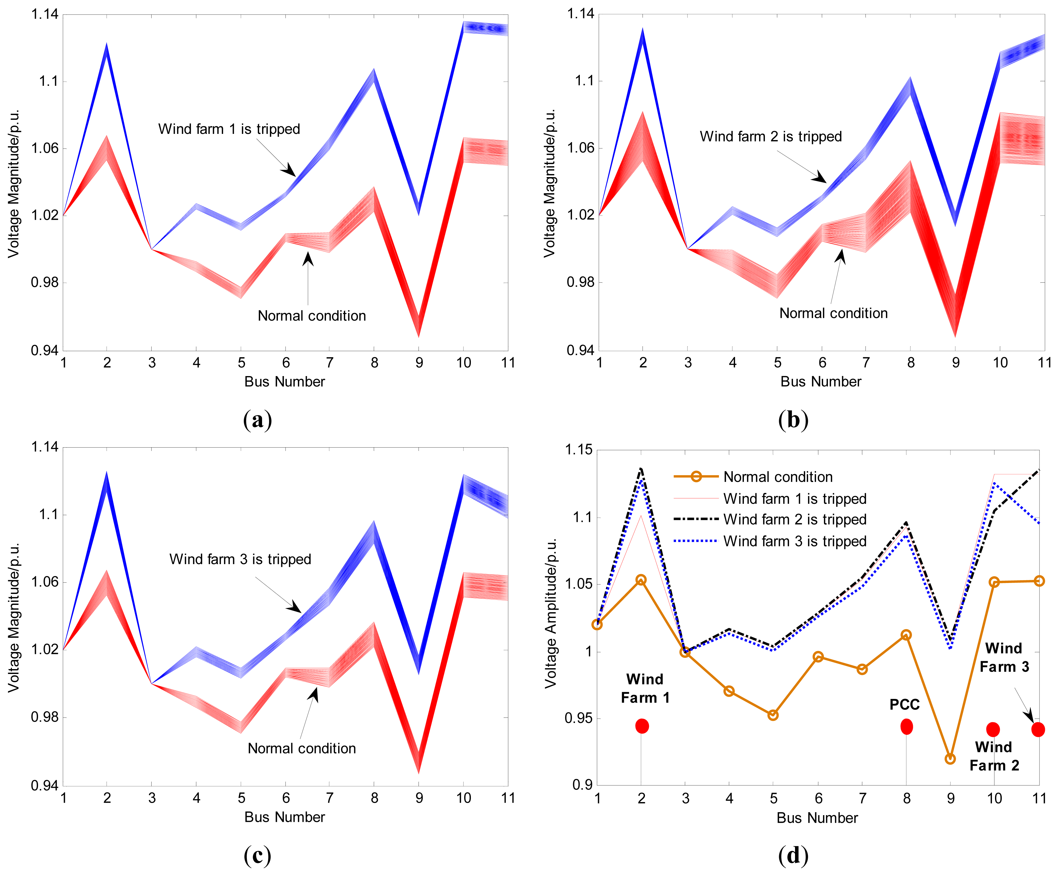
Suppose each wind farm total generation is given as P_w1 = [120, 140], P_w2 = [100, 120] and P_w3 = [80, 100]. It can be observed from Figure 6a–c that the voltage magnitude of each wind farm will exceeded the upper operational limit after N-1 contingency due to lower loading on the transmission lines and slow switch-off of the capacitance banks. The spiked voltages led to further tripping of other wind farms by the overvoltage protection system. Although the wind power output is still random after N-1 contingency, it is institutive that lower load will lead to higher spiked voltage magnitude. Therefore, we can choose that the worst case for further consideration, shown in Figure 6d, such that when one wind farm is tripped, the other wind farms' generation reach to their lowest possible generation.

For instance, if P_w1 is tripped, i.e., P_w1 = 0, the worst case is that P_w2 = 100 and P_w3 = 80. Note that the voltages at buses 1 and 3 do not change because bus 1 is a slack bus and bus 3 is a PV bus. It should be pointed out that the reactive power of PV bus should be also limited to its upper and lower bound, and the bus type is desired to be converted from PV type to PQ type if the reactive power reaches its bound. But in this study, the reactive power doesn't reach the bound so that it leads to a constant value both at normal condition and N-1 contingencies.

Table 3. Voltage magnitudes at wind farms under normal and N-1 contingency conditions (with/without capacitance cut-off).

Condition	Uw1	Uw2	Uw3	ratio	ratio	ratio
Normal	1.032	1.029	1.031	-	-	-
C1-on	1.095	1.126	1.127	6.10%	9.43%	9.31%
C1-off	1.055	1.095	1.096	2.23%	6.41%	6.30%
C2-on	1.125	1.092	1.124	9.01%	6.12%	9.02%
C2-off	1.099	1.059	1.099	6.49%	2.92%	6.60%
C3-on	1.114	1.112	1.080	7.95%	8.07%	4.75%
C3-off	1.096	1.094	1.055	6.20%	6.32%	2.33%

Note: Ci-on (i = 1,2,3) indicates that wind farm i is tripped, but the capacitance at this wind farm remains in service, whereas Ci-off indicates that the capacitance is cut off when the wind farm is tripped. Bold and underlined entries indicate voltage violations. Each ratio entry is the ratio of the voltage variation after a wind farm trip to normal conditions.

further compares the wind farm voltages in the case where the connecting capacitance is cut off and the case where the connecting capacitance remains in service. It is clear that when the capacitance is not cut off, the voltage magnitudes at the wind farms will increase sharply.

The voltage security region under N-1 contingency conditions will be calculated in the followed steps. Note that in the following calculations, capacitances are not cut off when a wind farm is tripped to represent a worst-case scenario.

• Step 1: Normal conditions

  Under normal conditions, the two near points are calculated as η_ξ+ = (14.04, 14.92, 15.88) and η_ξ− = (−5.66, −5.28, −4.78). The inner points associated with η_ξ+ are (0, 20.83, 21.80), (20.28, 0, 22.14), and (20.66, 21.55, 0), and those associated with η_ξ− are (0, −7.88, −7.39), (−8.07, 0, −7.19), and (−7.28, −7.44, 0). The security region boundary can then be represented by:

  $$\begin{array}{ll}{\mathcal{A}}^{0+}\hfill & =\left[\begin{array}{lll}0.0277\hfill & 0.0199\hfill & 0.0198\hfill \\ 0.0198\hfill & 0.0274\hfill & 0.0197\hfill \\ 0.0197\hfill & 0.0196\hfill & 0.0272\hfill \end{array}\right],{\mathcal{A}}^{0+}\left[\begin{array}{c}{Q}_{w1}\\ Q_{w2}\\ Q_{w3}\end{array}\right]\le \left[\begin{array}{c}1\\ 1\\ 1\end{array}\right]\hfill \\ {\mathcal{A}}^{0-}\hfill & =\left[\begin{array}{lll}0.0713\hfill & 0.0595\hfill & 0.0591\hfill \\ 0.0601\hfill & 0.0712\hfill & 0.0593\hfill \\ 0.0605\hfill & 0.0601\hfill & 0.0712\hfill \end{array}\right],{\mathcal{A}}^{0-}\left[\begin{array}{c}{Q}_{w1}\\ Q_{w2}\\ Q_{w3}\end{array}\right]\ge \left[\begin{array}{c}-1\\ -1\\ -1\end{array}\right]\hfill \end{array}$$

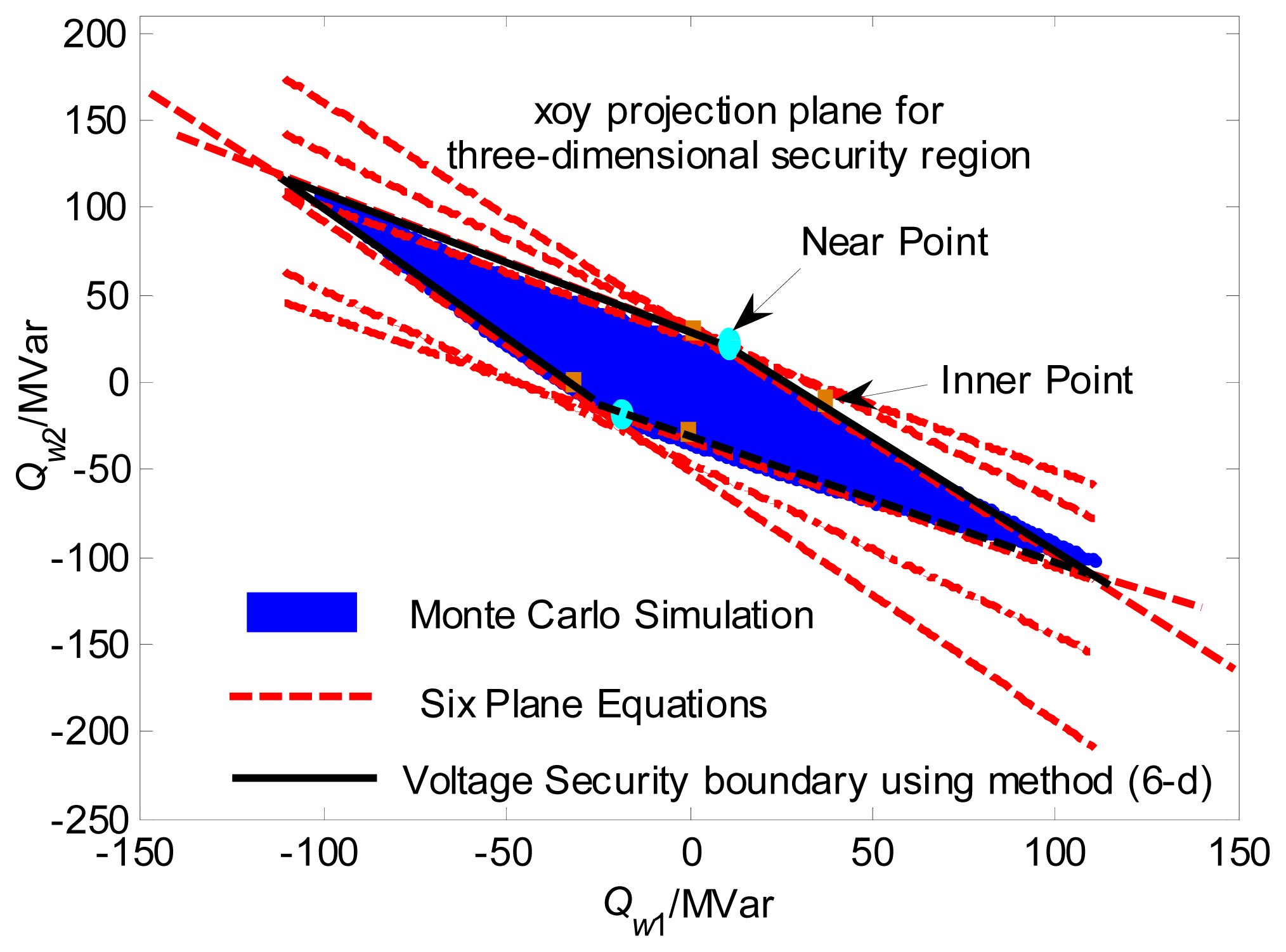
  With three wind farms, the voltage security region is a three-dimensional space. For illustrative purposes, only the projection of this three-dimensional space on the (Q_w1, Q_w2)-plane is shown in Figure 7. In this figure, the normal condition voltage security region obtained via method (6d) is indicated by the bold dotted line, and is the closure of twelve planes (dotted lines). The security region obtained via method (6c) is indicated by the bold solid line, and a comparison of the two regions shows that method (6d) outperforms method (6c) in boundary approximation.

• Step 2: When wind farm 1 is tripped

  When wind farm 1 is tripped, the two near points are η_ξ+ = (15.60, 8.13, 6.18) and η_ξ− = (−12.58, −26.09, −25.60). The inner points associated with η_ξ+ are (0, 4.95, 5.90), (15.14, 0, −0.64), and (15.52, −1.21, 0), and those associated with η_ξ− are (0, −31.10, −30.62), (−23.79, 0, −36.65), and (−23.50, −36.84, 0). The security region boundary under wind farm 1 tripping conditions can be written as:

  $$\begin{array}{ll}{\mathcal{A}}^{1+}\hfill & =\left[\begin{array}{lll}0.0683\hfill & 0.0490\hfill & 0.0521\hfill \\ 0.0728\hfill & 0.1069\hfill & 0.0798\hfill \\ 0.0706\hfill & 0.0729\hfill & 0.1084\hfill \end{array}\right],{\mathcal{A}}^{1+}\left[\begin{array}{c}{Q}_{w1}\\ Q_{w2}\\ Q_{w3}\end{array}\right]\le \left[\begin{array}{c}1\\ 1\\ 1\end{array}\right]\hfill \\ {\mathcal{A}}^{1-}\hfill & =\left[\begin{array}{lll}0.0197\hfill & 0.0146\hfill & 0.0145\hfill \\ 0.0129\hfill & 0.0189\hfill & 0.0134\hfill \\ 0.0129\hfill & 0.0136\hfill & 0.0189\hfill \end{array}\right],{\mathcal{A}}^{1-}\left[\begin{array}{c}{Q}_{w1}\\ Q_{w2}\\ Q_{w3}\end{array}\right]\ge \left[\begin{array}{c}-1\\ -1\\ -1\end{array}\right]\hfill \end{array}$$

• Step 3: When wind farm 2 is tripped

  When wind farm 2 is tripped, the two near points are η_ξ+ = (5.97, 16.65, 5.86) and η_ξ−= (−25.10, −11.20, −24.24). The inner points associated with η_ξ+ are (0, 16.26, 0.46), (5.54, 0, 7.37), and (−0.62, 17.00, 0), and those associated with η_ξ− are (0, −22.13, −35.02), (−29.58, 0, −28.73), and (−35.33, −21.59, 0). The security region boundary when wind farm 2 is tripped is therefore represented by:

  $$\begin{array}{ll}{\mathcal{A}}^{2+}\hfill & =\left[\begin{array}{lll}0.0952\hfill & 0.0623\hfill & 0.0641\hfill \\ 0.0413\hfill & 0.0603\hfill & 0.0414\hfill \\ 0.0608\hfill & 0.0590\hfill & 0.0900\hfill \end{array}\right],{\mathcal{A}}^{2+}\left[\begin{array}{c}{Q}_{w1}\\ Q_{w2}\\ Q_{w3}\end{array}\right]\le \left[\begin{array}{c}1\\ 1\\ 1\end{array}\right]\hfill \\ {\mathcal{A}}^{2-}\hfill & =\left[\begin{array}{lll}0.0202\hfill & 0.0133\hfill & 0.0142\hfill \\ 0.0157\hfill & 0.0207\hfill & 0.0155\hfill \\ 0.0145\hfill & 0.0138\hfill & 0.0199\hfill \end{array}\right],{\mathcal{A}}^{2-}\left[\begin{array}{c}{Q}_{w1}\\ Q_{w2}\\ Q_{w3}\end{array}\right]\ge \left[\begin{array}{c}-1\\ -1\\ -1\end{array}\right]\hfill \end{array}$$

• Step 4: When wind farm 3 is tripped

  When wind farm 3 is tripped, the two near points are η_ξ+ = (5.10, 5.98, 17.74) and η_ξ− = (−23.71, −23.34, −9.79). The inner points associated with η_ξ+ are (0, 1.02, 17.78), (0.50, 0, 18.14), and (7.05, 7.92, 0), and those associated with η_ξ− are (0, −33.56, −20.16), (−33.68, 0, −19.92), and (−27.65, −27.28, 0). The security region under this N-1 contingency is then given by:

  $$\begin{array}{ll}{\mathcal{A}}^{3+}\hfill & =\left[\begin{array}{lll}0.0806\hfill & 0.0545\hfill & 0.0529\hfill \\ 0.0525\hfill & 0.0795\hfill & 0.0517\hfill \\ 0.0364\hfill & 0.0370\hfill & 0.0541\hfill \end{array}\right],{\mathcal{A}}^{3+}\left[\begin{array}{c}{Q}_{w1}\\ Q_{w2}\\ Q_{w3}\end{array}\right]\le \left[\begin{array}{c}1\\ 1\\ 1\end{array}\right]\hfill \\ {\mathcal{A}}^{3-}\hfill & =\left[\begin{array}{lll}0.0210\hfill & 0.0153\hfill & 0.0146\hfill \\ 0.0155\hfill & 0.0210\hfill & 0.0147\hfill \\ 0.0167\hfill & 0.0167\hfill & 0.0219\hfill \end{array}\right],{\mathcal{A}}^{3-}\left[\begin{array}{c}{Q}_{w1}\\ Q_{w2}\\ Q_{w3}\end{array}\right]\ge \left[\begin{array}{c}-1\\ -1\\ -1\end{array}\right]\hfill \end{array}$$

• Step 5: N-1 voltage security region

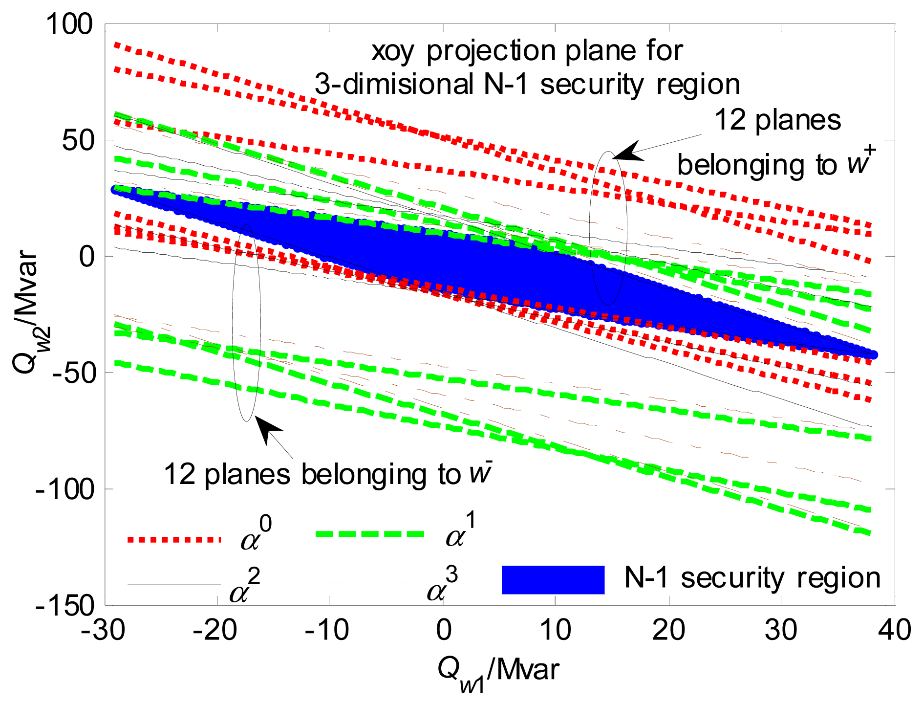
  The N-1 voltage security region can be expressed as $\underset{w=0}{\overset{3}{\text{∪}}}\left\{{\mathcal{A}}^{w-},{\mathcal{A}}^{w+}\right\}$. It is bounded by 24 planes, of which 12 are associated with w⁺ and the other 12 are associated with w⁻, as shown in Figure 8. With reactive power limits taken into account, the final N-1 voltage security region is $\underset{w=0}{\overset{3}{\text{∪}}}\left\{{\mathcal{A}}^{w-},{\mathcal{A}}^{w+}\right\}\cap Q_w^{lim}$, where:

  $${\text{Q}}_w^{lim}=\{\begin{array}{l}-67.8051\le Q_{w1}^{lim}\le 67.8051\\ -62.9619\le Q_{w2}^{lim}\le 62.9619\\ -58.1187\le Q_{w3}^{lim}\le 58.1187\end{array}$$

  It should be noted that although the N-1 security region shown in Figure 8 is similar in shape to the normal condition security region shown in Figure 7, it is actually a subset of the normal condition security region, and therefore significantly smaller. Coincidentally, in this case, the N-1 security region is entirely within the reactive power limits, whereas the normal condition security region is not. In Figure 8, there are 12 planes belonging to w⁺ and 12 planes belonging to w⁻. Each type of line represents a different contingency, and the intersection of these planes constitutes the N-1 security region; i.e., the reactive power within this region under normal conditions could guarantee security under both normal operation and an N-1 contingency.

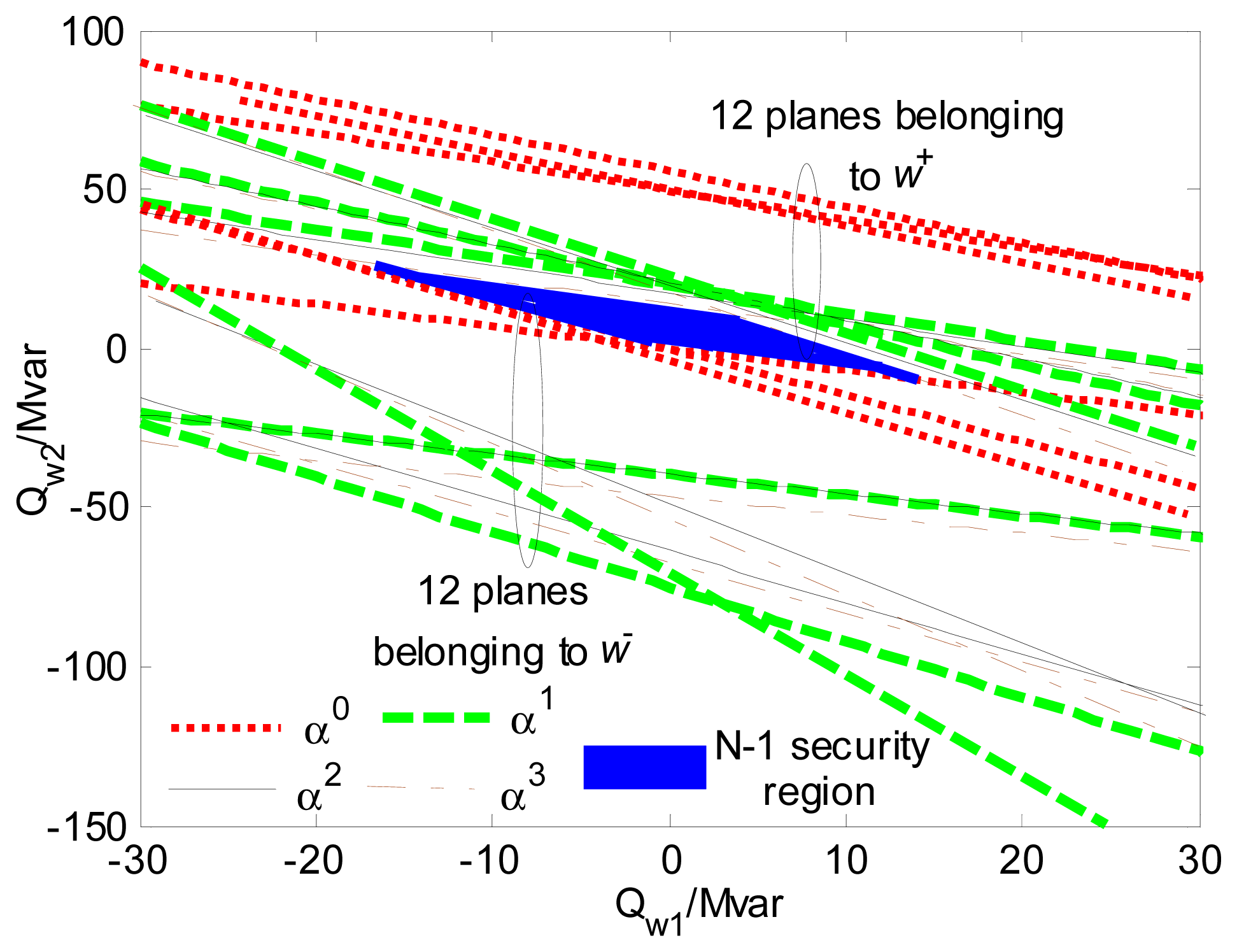
Last but not least, the N-1 voltage security region may not exist when wind penetration increases radically. Intuitively, the higher the penetration is, the greater the reactive power required to maintain the voltage in the safety region. If one wind farm is tripped at such a time, the voltage at each wind farm is certain to rise because of the slow switch-off of the capacitance banks, and may not remain inside the N-1 security region. In terms of the voltage security region, the area of the normal security region will decrease steadily with increasing penetration (see Table 2 and Figure 3). A comparison of Figures 7, and 9 also implies that the N-1 voltage security region may shrink, so that high penetration will shift the normal voltage security region further and further from the N-1 conditions (see Figure 9). Thus, if P_w increases from 0 MW, the area of the intersection decreases. The three indices defined in Equations (5)−(7) were calculated for different levels of wind power penetration, and the results are listed in

Table 4. Three indices for different levels of wind power penetration.

Penetration	Scenario	ηξ+	ηξ−	Iu	It	Is
	normal	(14.04, 14.92, 15.88)	(−5.66, −5.28, −4.78)	19.70	34.9709	1.00
Pw1 = 140 MW	w1 tripping	(15.60, 8.13, 6.18)	(−12.58, −26.09, −25.60)	10.96	54.5444	0.75
Pw2 = 130 MW	w2 tripping	(5.97, 16.65, 5.86)	(−25.10, −11.20, −24.24)	10.64	51.4488	0.73
Pw3 = 120 MW	w3 tripping	(5.10, 5.98, 17.74)	(−23.71, −23.34, −9.79)	10.64	52.2018	0.74
	normal	(17.30, 18.17, 19.14)	(−0.66, −0.35, 0.09)	17.96	32.0695	1.00
Pw1 = 196 MW	w1 tripping	(17.06, −0.33, 0.62)	(−10.67, −24.49, −24.06)	0.02	44.2918	0.54
Pw2 = 182 MW	w2 tripping	(0.01, 18.27, 1.81)	(−23.24, −9.09, −22.50)	0.67	43.3602	0.58
Pw3 = 168 MW	w3 tripping	(1.23, 2.09, 19.51)	(−21.65, −21.34, −7.47)	1.89	42.4309	0.62
	normal	(38.92, 39.65, 40.53)	(34.08, 33.89, 33.91)	4.84	10.0214	1.00
Pw1 = 224 MW	w1 tripping	(25.71, 5.69, 6.55)	(0.61, −13.90, −13.87)	−28.20	37.8253	-
Pw2 = 208 MW	w2 tripping	(7.07, 27.83, 8.64)	(−10.98, 3.41, −11.13)	−27.01	36.2352	-
Pw3 = 192 MW	w3 tripping	(9.23, 9.94, 30.02)	(−8.13, −8.32, 6.30)	−24.85	34.6040	-
	normal	(6.42, 7.93, 15.60)	(−15.00, −14.41, −9.11)	21.42	39.6040	1.00
Pw1 = 196 MW	w1 tripping	(11.17, −5.51, 2.08)	(−18.43, −31.85, −26.66)	8.90	48.9484	0.64
Pw2 = 130 MW	w2 tripping	(−1.57, 12.62, 6.52)	(−25.51, −16.48, −21.73)	11.43	47.0956	0.76
Pw3 = 60 MW	w3 tripping	(0.38, 1.88, 18.65)	(−22.75, −22.16, −8.59)	15.38	43.0690	0.83

. The following conclusions may be drawn.

(i)

Under normal conditions, I_u decreases with increasing wind power penetration. In particular, I_u would decrease further after an N-1 contingency. Thus, if I_u < 0, the area of the intersection would vanish, as in No. 3. This index can therefore be used to assess the existence of the voltage security region.

(ii)

Under normal conditions, I_t decreases with increasing wind power penetration. However, I_u would increase after an N-1 contingency. This index describes the approximate size of the voltage security region.

(iii)

I_t decreases with increasing wind power penetration, and would further decrease after an N-1 contingency. This index describes the approximate size of the intersection between normal conditions and the contingency.

(iv)

A wind farm with higher I_t has a higher risk of insecurity after tripping. Observe that when the three wind farms have distinct penetration levels (bottom section of Table 4), I_u is positive and I_t is far from 0 under each condition, so that the voltage security region exists. However, the minimum of I_s occurs when w₁ is tripped, and the maximum occurs when w₃ is tripped. Therefore, the insecurity risk of a w₁ trip is greater than that of w₃.

Curtailment is an effective method for restoring the N-1 security region. Accordingly, it should be implemented, and will be studied in future work.

4.2. Two-Step Optimal Adjustment Strategy

Assume that the voltage security region exists, and at a given operating point, the reactive power outputs of the three wind farms are (20, 20, 10) MVar. From Figure 7, the operating point is secure under normal conditions because it is within the voltage security region. However, when a single wind farm is tripped and the connecting capacitance is still in service, the operating point will be outside the N-1 security region, as Figure 8 shows. The wind farm voltages increase beyond their upper bounds, and thus the operating point moves into the insecure region. An adjustment strategy must be employed to return the operating point to the secure region.

The proposed two-step adjustment strategy is as follows: in the first step, shift the insecure operating point to the N-1 security boundary with minimum reactive power regulation. Then, in the second step, move the operating point toward the center of the security region, so that a security margin is maintained. Of course, minimum adjustment is only one of a number of effective strategies for adjusting an insecure operating point. Depending on the N-1 security region, various adjustments with various objectives could be employed.

Step 1:

Shift the insecure operating point to the security region boundary

The optimization model of Section 2 is:

$$\begin{array}{c}min{\left(Q_{w1}-20\right)}^2+{\left(Q_{w2}-20\right)}^2+{\left(Q_{w3}-10\right)}^2\\ \begin{array}{cc}s.t.{\mathbf{\alpha }}^{i+}\left(\begin{array}{c}{Q}_{w1}\\ Q_{w2}\\ Q_{w3}\end{array}\right)\le 1& {\mathbf{\alpha }}^{i-}\left(\begin{array}{c}{Q}_{w1}\\ Q_{w2}\\ Q_{w3}\end{array}\right)\ge -1i=0,1,2,3\end{array}\\ -67.8051\le Q_{w1}^{lim}\le 67.8051\\ -62.9619\le Q_{w2}^{lim}\le 62.9619\\ -58.1187\le Q_{w3}^{lim}\le 58.1187\end{array}$$

where α⁰⁺, α¹⁺, α²⁺, and α³⁺ were calculated in Section III. This quadratic programming problem can easily be solved, yielding an optimal objective value of 499.1831.

Step 2:

Shift the operating point from the boundary to the interior of the security region

Using the two near points calculated in Section III, we can obtain the reactive power range for determining the center of the security region. This range is different for each N-1 contingency condition. The intersection of the ranges is $\{\begin{array}{l}-5.66\le Q_{w1}\le 5.10\\ -5.28\le Q_{w2}\le 5.98\\ -4.78\le Q_{w3}\le 5.86\end{array}$. Then, using Equation (28) of [1], the center of the security region can be calculated as O_a = (−0.28, −0.35, −0.5).

The voltage magnitudes at the wind farms before/after adjustment are compared in

Table 5. Comparison of the voltage magnitudes at the wind farms under normal and N-1 contingency conditions before/after adjustment.

Adjustment Strategy	Condition	Uw1 (p.u.)	Uw2 (p.u.)	Uw3 (p.u.)
Without adjustment	Normal	1.032	1.029	1.031
	w1 tripping	1.095	1.126	1.127
	w2 tripping	1.125	1.092	1.124
	w3 tripping	1.114	1.112	1.080
Step 1 (minimum adjustment)	Normal	0.985	0.994	0.985
	w1 tripping	1.079	1.101	1.094
	w2 tripping	1.088	1.081	1.089
	w3 tripping	1.089	1.097	1.074
Step 2 (center adjustment)	Normal	0.954	0.963	0.954
	w1 tripping	1.065	1.080	1.078
	w2 tripping	1.074	1.059	1.075
	w3 tripping	1.067	1.068	1.054

. Under normal conditions, the voltage magnitudes are within limits. However, when one of the wind farms is tripped, the voltage magnitudes at some wind farms exceed their upper bounds, indicating that the original operating point is not within the N-1 voltage security region. After the first optimal adjustment step has been taken, the operating point moves to the N-1 voltage security boundary. For instance, when wind farm w1 is tripped, U_w2 reaches 1.101 p.u., slightly exceeding the upper bound of 1.1 p.u., due to the error introduced by using linear security region boundary components to approximate the actual nonlinear boundary components. Nevertheless, the corresponding reactive power remains quite close to the security region boundary.

Moreover, thanks to the larger security margin obtained in the second step of the center-adjustment strategy, U_w2 is lowered to 1.080 p.u. when wind farm w₁ is tripped, which is well under the upper bound 1.1 p.u. Hence, the corrected operating point is completely within the N-1 voltage security region.

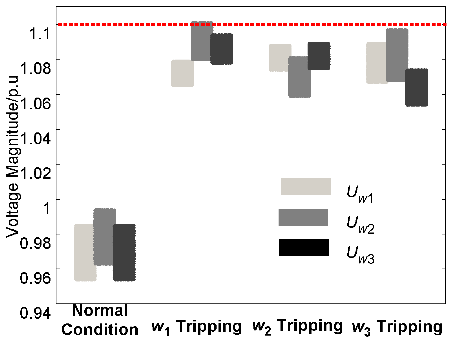
At the same time, the adjustable voltage range under normal conditions lies between the results of step 1 and step 2; i.e., U_w1 = [0.954, 0.985], U_w2 = [0.963, 0.994], and U_w3 = [0.954, 0.985]. To further illustrate the effectiveness of the adjustable voltage range in the minimum-adjustment and center-adjustment models, 10,000 operating point samples (in the form of reactive power) from the center to the minimum-adjustment point were randomly generated by Monte Carlo simulation and tested. The voltage magnitude distribution was easily obtained from the power flow, and is shown in Figure 10 before and after wind farm tripping. As an interesting example, note that when wind farm i was tripped, the voltage magnitudes of all wind farms increased, but the voltage U_i varied less than that of the other wind farms.

5. Conclusions

Based on the concepts and technique proposed in [1], a number of observations were made. First, simply operating below the reactive power limits does not guarantee that voltages will remain within limits, and hence a voltage security region is a must. Second, higher wind penetration leads to a higher degree of nonlinearity of the security region boundary components. Third, the size of the security region diminishes with increasing wind penetration.

The effect of wind farm tripping was also examined. Wind farm voltages will increase significantly when a wind farm is tripped if the connecting capacitance is not cut off. An optimal adjustment strategy was demonstrated on an insecure operating point outside the N-1 security region. The minimum-adjustment correction model was used to shift the point to the boundary of N-1 security region, and ultimately the adjustable voltage range of each wind farm was obtained under normal conditions.

The proposed voltage security region and adjustment strategy can be used to achieve better coordination among wind farm reactive power controls, and help prevent cascading tripping following a single wind farm trip. However, the N-1 voltage security region shrinks to the vanishing point when wind penetration increases radically. Curtailment is an effective method of restoring the security region, and will be studied in future work.

References

- Ding, T.; Guo, Q.; Bo, R.; Sun, H.; Zhang, B. A static voltage security region for centralized wind power integration—Part I: Concept and method. Energies 2014, 7, 420–443. [Google Scholar]
- Ding, T.; Guo, Q.; Sun, H.; Wang, B.; Xu, F. A Quadratic Robust Optimization Model for Automatic Voltage Control on Wind Farm Side. Proceedings of the IEEE Power and Energy Society General Meeting (PES), Vancouver, BC, Canada, 21–25 July 2013; pp. 1–5.
- Bracale, A.; Carpinelli, G.; Proto, D.; Russo, A.; Varilone, P. New approaches for very short-term steady-state analysis of an electrical distribution system with wind farms. Energies 2010, 3, 650–670. [Google Scholar]
- Pierik, J.; Axelsson, U.; Eriksson, E.; Salomonsson, D.; Bauer, P.; Czech, B. A wind farm electrical systems evaluation with EeFarm-II. Energies 2010, 3, 619–633. [Google Scholar]
- Torchyan, K.; Elmoursi, M.S.; Xiao, W. Adaptive Secondary Voltage Control for Grid Interface of Large Scale Wind Park. Proceedings of the 2013 IEEE Grenoble PowerTech (POWERTECH), Grenoble, France, 16–20 June 2013.
- Liu, Y.; Chen, Z. Voltage Sensitivity Based Reactive Power Control on VSC-HVDC in a Wind Farm Connected Hybrid Multi-Infeed HVDC System. Proceedings of the 2013 IEEE Grenoble PowerTech (POWERTECH), Grenoble, France, 16–20 June 2013.
- Heredia, E.; Kosterev, D.; Donnelly, M. Wind Hub Reactive Resource Coordination and Voltage Control Study by Sequence Power Flow. Proceedings of the IEEE Power and Energy Society General Meeting, Vancouver, BC, Canada, 21–25 July 2013; pp. 1–5.
- Zheng, T.Y.; Jiao, S.H.; Ding, K.; Lin, L. A Coordinated Voltage Control Strategy of Wind Farms Based on Sensitivity Method. Proceedings of the 2013 IEEE Grenoble PowerTech (POWERTECH), Grenoble, France, 16–20 June 2013.
- Kabouris, J.; Kanellos, F.D. Impacts of large scale wind penetration on energy supply industry. Energies 2009, 2, 1031–1041. [Google Scholar]
- Akhmatov, V.; Eriksen, P.B. A large wind power system in almost island operation—A Danish case study. IEEE Trans. Power Syst. 2007, 22, 937–943. [Google Scholar]
- Tapia, G.; Tapia, A.; Ostolaza, J.X. Proportional—Integral regulator-based approach to wind farm reactive power management for secondary voltage control. IEEE Trans. Power Syst. 2007, 22, 488–498. [Google Scholar]
- Cezar Rabelo, B.; Hofmann, W.; da Silva, J.L.; de Oliveira, R.G.; Silva, S.R. Reactive power control design in doubly fed induction generators for wind turbines. IEEE Trans. Ind. Electron. 2009, 56, 4154–4162. [Google Scholar]
- Diaz-Dorado, E.; Carrillo, C.; Cidras, J. Control algorithm for coordinated reactive power compensation in a wind park. IEEE Trans. Energy Convers. 2008, 23, 1064–1072. [Google Scholar]
- Qiao, W.; Venayagamoorthy, G.K.; Harley, R.G. Coordinated reactive power control of a large wind farm and a STATCOM using heuristic dynamic programming. IEEE Trans. Energy Convers. 2009, 24, 493–503. [Google Scholar]
- Martinez, J.; Kjær, P.C.; Rodriguez, P.; Teodorescu, R. Design and analysis of a slope voltage control for a DFIG wind power plant. IEEE Trans. Energy Convers. 2012, 27, 11–20. [Google Scholar]
- Hu, J.B.; He, Y.K. Reinforced control and operation of DFIG-based wind-power-generation system under unbalanced grid voltage conditions. IEEE Trans. Energy Convers. 2009, 24, 905–915. [Google Scholar]
- Konopinski, R.J.; Vijayan, P.; Ajjarapu, V. Extended reactive capability of DFIG wind parks for enhanced system performance. IEEE Trans. Power Syst. 2009, 24, 1346–1355. [Google Scholar]
- Sun, H.; Guo, Q.; Zhang, B.; Wu, W.; Wang, B. An adaptive zone-division-based automatic voltage control system with applications in China. IEEE Trans. Power Syst. 2013, 28, 1816–1828. [Google Scholar]
- Guo, Q.L.; Sun, H.; Zhang, M.; Tong, J.; Zhang, B.; Wang, B. Optimal voltage control of PJM smart transmission grid: Study, implementation, and evaluation. IEEE Trans. Smart Grid 2013, 4, 1665–1674. [Google Scholar]
- Guo, Q.L.; Sun, H.; Liu, Y.; Chen, R.; Wang, B.; Zhang, B. Distributed Automatic Voltage Control Framework for Large-scale Wind Integration in China. Proceedings of the 2012 IEEE Power and Energy Society General Meeting, San Diego, CA, USA, 22–26 July 2012; pp. 1–5.
- MATPOWER. Available online: http://www.pserc.cornell.edu/matpower/ (accessed on 26 November 2013).
Nomenclature