Can Tidal Current Energy Provide Base Load?


Department of Electronic Engineering, National University of Ireland, Maynooth, Co. Kildare, Ireland
*
Authors to whom correspondence should be addressed.
Energies 2013, 6(6), 2840-2858; https://doi.org/10.3390/en6062840
Submission received: 11 March 2013
/
Revised: 31 May 2013
/
Accepted: 3 June 2013
/
Published: 14 June 2013
(This article belongs to the Special Issue Energy from the Ocean - Wave and Tidal Energy)
Abstract
:Tidal energy belongs to the class of intermittent but predictable renewable energy sources. In this paper, we consider a compact set of geographically diverse locations, which have been assessed to have significant tidal stream energy, and attempt to find the degree to which the resource in each location should be exploited so that the aggregate power from all locations has a low variance. An important characteristic of the locations chosen is that there is a good spread in the peak tidal flow times, though the geographical spread is relatively small. We assume that the locations, all on the island of Ireland, can be connected together and also assume a modular set of tidal turbines. We employ multi-objective optimisation to simultaneously minimise variance, maximise mean power and maximise minimum power. A Pareto front of optimal solutions in the form of a set of coefficients determining the degree of tidal energy penetration in each location is generated using a genetic algorithm. While for the example chosen the total mean power generated is not great (circa 100 MW), the case study demonstrated a methodology that can be applied to other location sets that exhibit similar delays between peak tidal flow times.
1. Introduction
The strong tidal currents surrounding the Irish coast are a potential energy resource for the production of electricity, where the kinetic energy of the water stream is converted by tidal devices into electrical energy. Tides are locally pulsing energy sources resulting from astronomical movements of the Earth–Moon–Sun system. For this reason, the installation of a large set of tidal devices only in a single location creates a large variation in the amount of generated energy over a tidal cycle. A peak of energy, corresponding to maximum tidal flow, is available about every six hours and thirteen minutes, and between two peaks it is common to have a minimum with no energy production. This strong variation is a disadvantage for the production of electricity; indeed, it is important from the point of view of the scheduling and dispatch of power stations to have power sources with low variance during the day.
A crucial aspect of tidal streams around Ireland is that different locations along the coast experience peaks of water velocity at different times. When the water velocity in a location is zero, the water velocity in another location may have a considerable value. This difference of phase between locations has the potential to compensate the unwanted pulsing nature of tides and to smooth the total instantaneous generated power by adding the energy generated by different tidal farms at distributed locations. Because of their astronomical nature, tides have a very predictable time evolution, foreseeable for decades with an accuracy close to 98% [1]. It is specifically this deterministic property that makes tidal energy different from other types of renewable energy (most of which are not predictable with high levels of accuracy) and provides an interesting opportunity for its integration into the national electric grid. It is important to verify that it is possible to create a minimum constant supply of power to the national electric grid, by installing tidal farms in appropriate locations, and in a suitable quantity. In theory, the supply of energy drawn from an appropriate set of tidal farms would be reliable enough to replace some of the gas and oil power stations.
The main objectives of the current paper are: (a) to identify the locations for the installation of the turbines; (b) to quantify the energy available in each location; (c) to quantify the tidal stream velocity in each location; and (d) to quantify the fraction of energy that has to be utilised in each location with an optimisation criteria in order to minimise total variability.
2. Tides Analysis and Modelling
The cyclical rise and fall of the tides is caused by two principal factors: gravitational attraction (mainly by the Moon and the Sun) and inertial effects related to the Earth’s rotation [2,3]. From the theory of continuous time signals, it is known that it is possible to use Fourier analysis to represent periodic signals as the superimposition of a set (possibly infinite) of sine functions having frequencies that are multiples of the fundamental frequency. Since tides are created by astronomic events having periodic repetitions, tides can also be described as a summation of sine functions but with the important difference that in this case the frequency of the harmonic constituents are not always related to each other with integer factors. The level of the sea (or equivalently, the orthogonal velocity components of the tidal current) can be represented by [3,4,5]:
where is the constant constituent; N is the number of harmonic constituents; are the magnitudes; are the angular frequencies; are the periods and are the phases. Experiments have shown that more than 100 harmonic constituents influence the evolutions of tides, but the majority of them have too small a magnitude to be significant [6]. Because the tides are strongly influenced by Earth geographical position, the most relevant harmonic constituents change with location. To describe the tides in North Europe, in the tidal atlas [7,8], the simplified harmonic method of tidal prediction utilises the 4 harmonic constituents , , and (Table 1). In the current work we retain sufficient the accuracy obtained utilising the same 4 harmonic constituents , , and , considering that:
- (a)
- The turbine curves utilised for the simulations of the current article are 3 idealised curves (no public real device curves were available);
- (b)
- The data available for the velocities at the different locations are calculated with the ROMS Irish Marine Institute’s hydrodynamic model, which is not able to provide highly accurate velocities for the narrow passage where the turbines are located [9].

| Harmonic constituent | Period (h) | Frequency (Rad/h) |
|---|---|---|
| Main solar semidiurnal (S2) | 12.0000 | 0.5236 |
| Main lunar semidiurnal (M2) | 12.4206 | 0.5059 |
| Lunar-solar declinational diurnal (K1) | 23.9344 | 0.2625 |
| Lunar declinational diurnal (O1) | 25.8194 | 0.2434 |
The relevant uncertainty introduced by (a) and (b) does not justify a number of harmonic constituents in Equation (1) bigger than four.
3. Tidal Currents
The time-dependent change in water level depending on tides causes the creation of compensating tidal currents that move water from one zone to another. In the open ocean, where the water is deep and there are no constraints for the water flow, the tidal current is in phase with the change of the water level. When the tide approaches the land, the phase between water height and current velocity changes under the influences of topographical features like restricted water depth and configuration of the coast [2].
Depending on their characteristics, tidal currents can be classified as [5]:
- Rotary currents: usually in the open ocean and along the sea coasts where the currents change both in direction and speed due the effect of the Coriolis force [5,10]. In case of semidiurnal tides, the current completes a rotation in about 12 h and 25 min (12.42 h). In case of diurnal tides, the current completes a rotation in about 24 h and 50 min (24.84 h).
- Rectilinear (reversing) currents: usually in straits or inland bodies of water, like rivers or bays, where the water, constrained by channel configuration, flows approximately in a rectilinear pattern [4,10]. During the flow in each direction the speed changes from zero (slack water) to a maximum and then back to zero again. For convention the flow upstream or toward shore is called flood and the flow downstream or away from the shore is called ebb [2]. In case of a perfect semidiurnal tidal stream, both flood and ebb last about 6 h and 13 min but, in the case of either a diurnal inequality or a non-tidal current, the duration and the dynamics of flood and ebb may be different. Around the cost of Ireland, the current can be considered semidiurnal [8].
The harmonic decomposition utilised for the water level is used also for tidal stream. In this case, the velocity is divided in two orthogonal components (usually eastward flow and northward flow, represented with x and y respectively) and each of these components is represented with a harmonic series [5,11]. The harmonic decomposition of the x component of the velocity is:
Similarly, the harmonic decomposition of the y component of the velocity is:
where , are the constant constituents (in case there is a non-tidal stream superimposed on the tidal one); N is the number of harmonic constituents; and are the magnitudes; are the angular frequencies; are the periods; and are the phases. In each location, the magnitude of the total velocity is given by the resultant of the orthogonal velocity components:
4. Site Characteristics
A very important part is the assessment of the tidal resource to identify the possible farm locations, the characteristics of the tidal stream velocities and the maximum extractable energy. Our approach is based on the fragmentation of ocean, seas and rivers into sectors small enough to consider a homogeneous velocity in each point of the sector. In each sector, the maximum extractable energy per year depends on the local tidal streams, coast morphology and environmental aspects [12]. Different types of information have been analysed to develop the tools required for the tidal resource quantification, such as simulations from hydrodynamic models [9], tidal atlas and tables [7,8,13,14,15], technical reports [12,16,17], Irish Sailing Directions [18,19] and the Irish Sea Pilot [20].
4.1. Tidal Resource Mapping
A report documenting tidal resources in Ireland is analysed in order to identify possible locations for tidal devices [12]. First of all, the gross energy content of marine currents has been estimated in the area delimited by the 10 metre depth contour and the 12 nautical mile territorial limit. The total theoretical energy available is 230,000 GWh/yr. The criteria below are applied to determine a selection of the possible practical locations:
- Minimum tidal current velocity of 2.0 m/s;
- Seabed compatible with the existing turbine support structure technology;
- Location limited by wave exposure, shipping lines, military zones and disposal sites;
- Compatible economic and commercial constraints, such as development costs and market incentives.
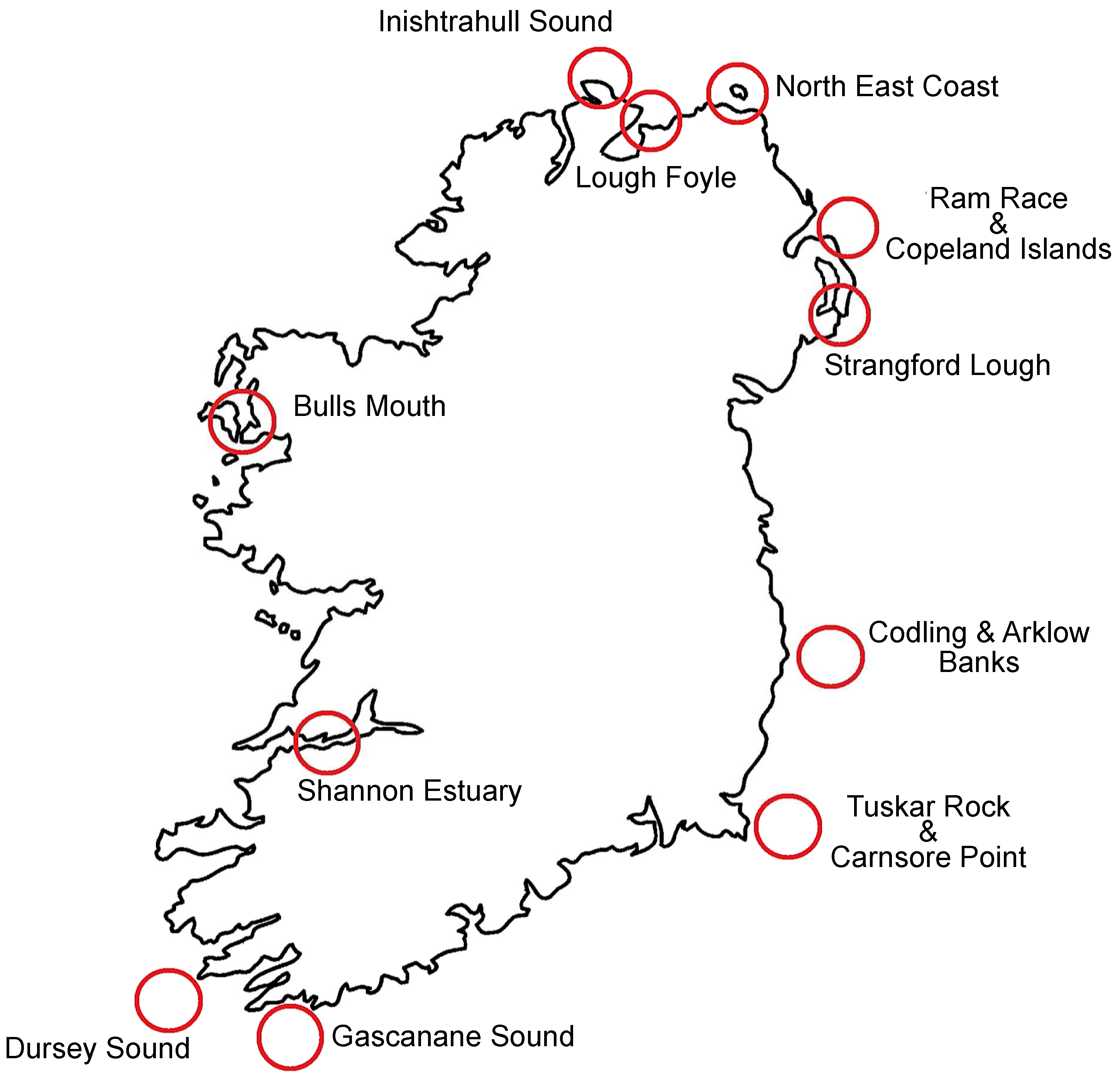
At the end, 11 locations were selected [12]. These locations are shown in Figure 1. The work of Garret and Cummins [21] showed that the installation of tidal turbines in a channel creates an alteration of the original undisturbed water flow, reducing the speed of the current. This means that it is necessary to take in consideration turbine array locations and turbine array layouts in order to calculate the viable resource [22]. As shown in [12], the Roberts Gordon Institute has undertaken some numerical studies for the locations of Inishtrahull Sound, Codling & Arklow Banks, Tuskar Rock & Carnsore Point and the Shannon Estuary in order to determine the viable resource [22]. Bathymetric data, current velocity and distances between the turbine rotors have been taken into account to assess each site for the most suitable number of turbines that could be installed. These studies provided the turbine array layouts and the total amount of viable energy that is possible to extract from each location (Table 2) [12,22]. The total amount of viable energy in one year is evaluated as 914 GWh/yr.
Figure 1.
SEI locations map.

In the current article, the viable energy represents the only constraint that can limit the number of installed devices in a specific location. The amount of energy extracted from each location has to be less than or equal to the viable energy in that location. We want to underline that, in the current article, the numbers utilised for the viable energy are mainly a working hypothesis to run the numerical example and that our most important objective is to show a methodology to employ multi-objective optimisation to simultaneously minimise variance, maximise mean power and maximise minimum power. We appreciate that the introduction of an explicit specific interaction between the number of installed turbines in a location and the reduction of the tidal stream velocity would provide a more realistic quantification of the amount of extractable energy in each location. However, for brevity, we use the interaction that is implicit in the viable power figures reported, since the focus of our work is not on resource modelling.
Table 2.
Viable energy at the different locations. Data from [12].
| Location | Available energy (GWh/yr) |
|---|---|
| Codling & Arklow Banks | 70 |
| Dursey Sound | 4 |
| Gascanane Sound | 1 |
| Inishtrahull Sound | 15 |
| North East Coast | 273 |
| Ram Race & Copeland Islands | 125 |
| Shannon Estuary | 111 |
| Tuskar Rock & Carnsore Point | 177 |
| Lough Foyle | 2 |
| Strangford Lough | 130 |
| Bulls Mouth | 6 |
4.2. Data Employed
4.2.1. ROMS Hydrodynamic Model
The Irish Marine Institute provided the data requested specifically for the current work [9], from the 1st of January 2012 to the 31st of January 2012 (one month) utilising the ROMS (Regional Ocean Modelling System) hydrodynamic model. For each location the orthogonal velocity components and are provided every 10 m (they are depth-averaged currents as an average for the whole water column). The magnitude of the total velocity is calculated with Equation (4). The stream velocities for Codling & Arklow Banks, Inishtrahull Sound, North East Coast, Ram Race & Copeland Islands and Tuskar Rock & Carnsore Point provided by the Marine Institute have been compared with the predictions obtained for the same locations, utilising the Tidal Stream Atlas [13,14,15]. Both magnitude and phase showed good agreement at the different locations. Furthermore, the performance of the ROMS hydrodynamic model is constantly monitored by the Marine Institute utilising real-world measurements [23]. An important characteristic of a good tidal energy site is the high velocity of the tidal stream (>2 m/s), and this happens commonly in very narrow sea straits. Unfortunately the horizontal grid resolution utilised by the ROMS hydrodynamic model is 1.2 km, not high enough to resolve the equations inside small passages. For this reason, the Marine Institute was only able to provide the velocities close to 7 of the 11 locations indicated by the SEI report: Inishtrahull Sound, Codling & Arklow Banks, Dursey Sound, Gascanane Sound, Northeast Coast, Ram Race & Copeland Islands and Tuskar Rock & Carnsore Point. Because the data are provided for locations that are not exactly inside the straits, their velocities are lower than the predicted ones in [12]. To resolve this mismatch, the velocities at Dursey Sound, Gascanane Sound and Ram Race & Copeland Islands are scaled by multiplying them by constants obtained from [18,19], to obtain the correct maximum speed at spring tides. The maximum velocities are, respectively, 2.058 m/s, 2.058 m/s and 2.572 m/s. For Bulls Mouth no data from the Marine Institute are available; for this reason, the velocity profile at this location is calculated, from 1st of January 2012 to the 31st of December 2012, utilising magnitude and phase available for Bulls Mouth in [19], together with the velocity “shape” available for Inishtrahull Sound from the Marine Institute.
4.2.2. Harmonic Identification with Least Squares
The amplitude and phase, of the constituents of the velocity in the harmonic series of Equations (2) and (3), are strongly influenced by the morphology of the coasts and sea floor with very complex relationships. Therefore the amplitude and phase of each harmonic constituent are often calculated empirically from observed data. A well-established procedure utilises curve fitting with least squares [5,24,25,26,27]. As explained in Section 2, we approximate each orthogonal velocity components and as summation of a constant and four harmonic constituents at different frequencies (Table 1). First of all, we calculated the average values:
and we found that both and are zero at each location. Consequently our fitting curve is:
where the coefficients and are the unknowns. We suppose that M couples of data , ,..., are available from measurement or simulations. At every instant , it is possible to calculate the distance (the error) of the curve from the real value :
represented by ,where is the vector of unknowns. We now define a total error function constructed as an addition of the single squared errors . The problem is to find the best that minimises S. This is a Least Squares Problem linear in the parameters and it is possible to show that the vector that minimises the vector of errors is [27]:
The summation of cosines and sines in (6) can be transformed into a summation of cosines only:
using the relationships:
Utilising Equations (9), (10) and (11) with the data provided by the Irish Marine Institute, the value of the two orthogonal components are extrapolated for the period from 1st January 2012 to 31st December 2012 for the 7 locations listed in Section 4.2.1:
4.2.3. Tidal Stream Atlas
Important sources of data regarding tidal current velocity are available in the Tidal Stream Atlas [13,14] where 13 maps are provided at hourly intervals for a given area. The maps utilised for the current paper start 6 h before High Water (HW) in the Standard Port of Dover (UK) and they finish 6 h after HW in Dover. Some definitions are necessary in order to understand how to utilise these atlases:
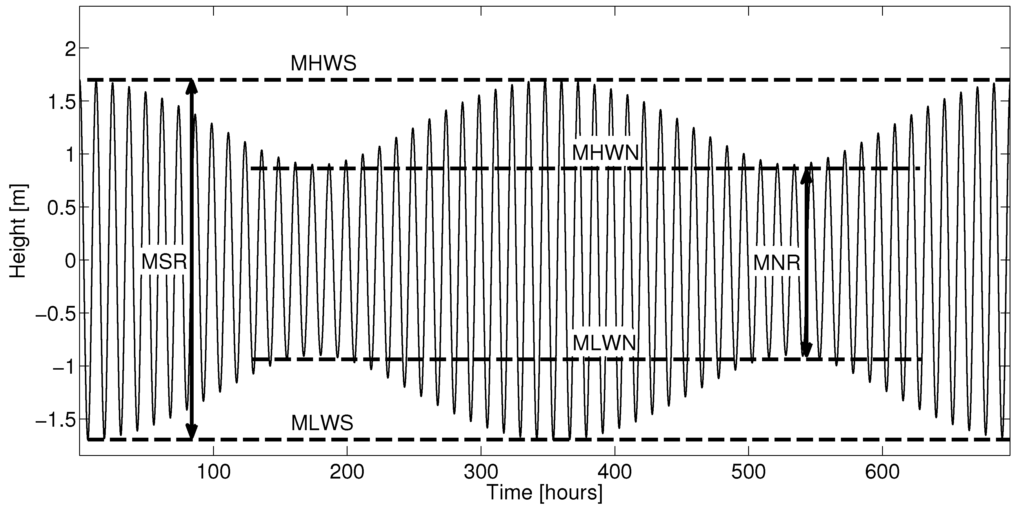
- Mean High Water Springs (MHWS) is calculated in a period of one year when the average maximum declination of the Moon is and it is equal to the average high water of two successive high waters during Spring periods of 24 h. In this case the range of tide isgreatest [8].
- Mean Low Water Springs (MLWS) is calculated in a period of one year when the average maximum declination of the Moon is and it is equal to the average low water of two successive low waters during Spring periods of 24 h. In this case the range of tide is greatest [8].
- Mean High Water Neaps (MHWN) is calculated in a period of one year when the average maximum declination of the Moon is and it is equal to the average high water of two successive high waters during Neap periods of 24 h. In this case the range of tide is least [8].
- Mean Low Water Neaps (MLWN) is calculated in a period of one year when the average maximum declination of the Moon is and it is equal to the average low water of two successive low waters during Neap periods of 24 h. In this case the range of tide is least [8].
- Mean Spring Range (MSR) = MHWS − MLWS [28].
- Mean Neap Range (MNR) = MHWN − MLWN [28].
See Figure 2 for a graphical representation.
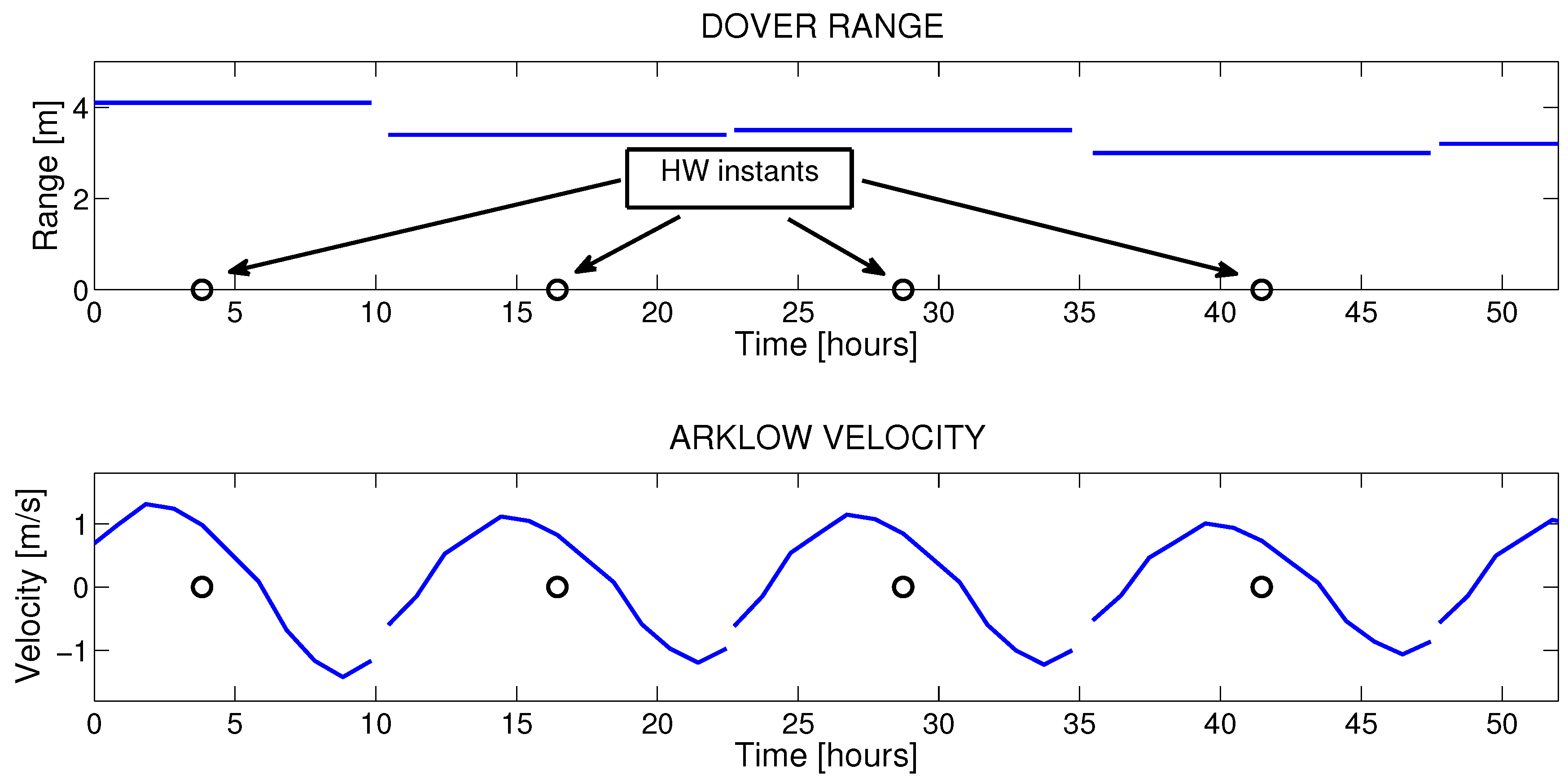
In each map, for a specific location, the mean Neap velocity (occurring in Dover when the water range is equal to its MSR, which is 6.0 m [15]) and the mean Spring velocity (occurring in Dover when the water range is equal to its MNR, which is 3.2 m [15]) are provided. For all the other cases, when the range in Dover is different from MSR or MNR, it is necessary to do a linear interpolation between these two values [29]:
where represents the water level range in Dover. Equation (13) is an algebraic model that illustrates the relationship between the water range at the utilised standard port (in this case Dover) and the location where the velocity is requested. If the values SpringVel and NeapVel are changed, it is possible to calculate the velocities at different locations. The calculated velocities (13 points in each time slot of about 12 h and 25 m) are aligned with the HW Dover time (Figure 3).
Figure 2.
Water height definitions.

Figure 3.
Water height range at Dover and calculated velocity at Arklow Bank (1st and 2nd of January 2012).
Figure 3.
Water height range at Dover and calculated velocity at Arklow Bank (1st and 2nd of January 2012).

Utilising Equation (13) and the data available in [13,15], the velocity profile for Lough Foyle is calculated from 1st of January 2012 to the 31st of December 2012.
For the Shannon Estuary and the narrows of Strangford Lough no tidal stream atlas data are available. For this reason, the velocity profile at these locations are calculated, from 1st of January 2012 to the 31st of December 2012, utilising magnitude and phase data available for the Shannon Estuary and narrows of Strangford Lough in [18,19,20], together with the velocity “shape" calculated with Equation (13) at Lough Foyle. Because Lough Foyle, Strangford Lough and the Shannon Estuary are inland straits, we assumed that the velocity profiles at the three locations are the same, but with different amplitudes and phases.
5. Turbine Modelling
The conversion of the kinetic energy of a tidal stream to electrical power requires the installation of tidal devices. In the current article, the tidal devices utilised are similar to marine versions of the well-established horizontal-axis wind turbines. The amount of instantaneous kinetic energy available in the tidal stream is equal to , where is the seawater density, A is the cross-sectional area swept by the rotor and is the velocity of the water stream. The marine turbine is able to extract only a part of this energy depending on its technical characteristics:
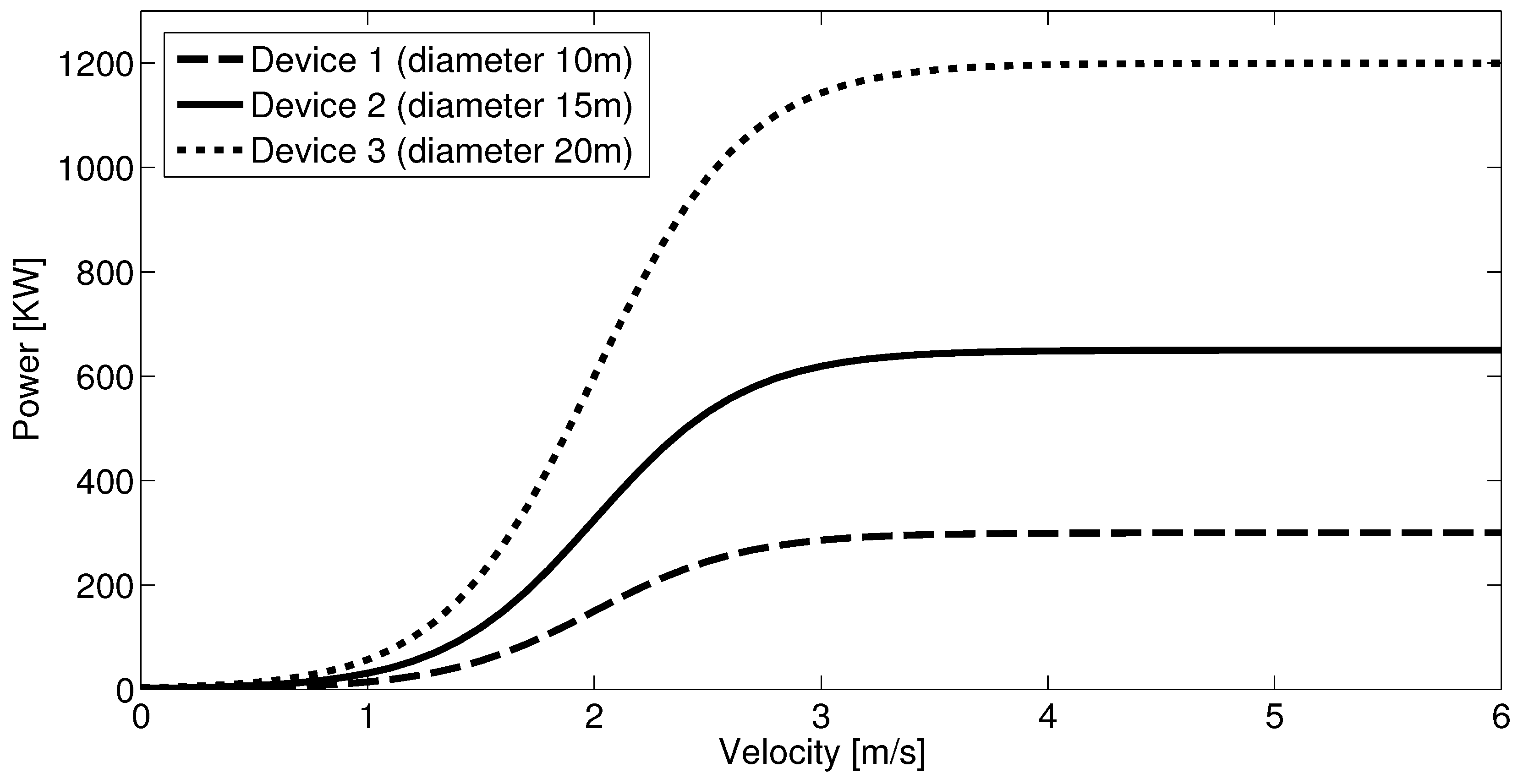
where is the power coefficient and represents the fraction of power that the device is able to extract from the water [1]. is a function of the blade pitch angle β and the tip speed ratio λ. Betz’s law states that the maximum amount of energy extracted by the device is [12,30]. A theoretical power coefficient, , of 0.45 was assumed for the tidal turbines, following the analysis in [31]. However, the actual power coefficient is, in fact, less than that due to the parameterisation of the turbine power curves, as shown in Figure 4. The introduction of automatic control technologies (like pitch control) provides the possibility to model the marine device with an algebraic relationship between velocity and extracted power .
Figure 4.
Device curves utilised for the simulations in the current paper.

The simulation model of the turbines and power distribution is based on the following hypothesis:
- The turbines are able to rotate in azimuth to follow the change of direction of the tidal currents; therefore the turbines are always aligned along the direction of maximum stream velocity.
- The device curves are assumed to be algebraic.
- We do not apply any constraint on the size and number of devices fitting into the selected areas (i.e., it is possible to install any number of devices that allows an extraction of energy per year smaller or equal than the viable energy).
- No power loss exists between the turbine and the final users (transmission and distribution with 100% efficiency).
The turbine starts generating power as the tidal current velocity crosses its cut-in speed. The power increases with the water stream speed up to the rated speed at which point the turbine generates its rated power . With a stream velocity between and cut-out velocity the power generated is constant. For safety reasons, the turbine is stopped for stream velocities higher than the cut-out speed [32].
The curves of the three turbines utilised in the current paper are shown in Figure 4, and the value of their parameters , , cut-in speed, cut-out speed and diameter are showed in Table 3.
| Parameter | Turbine 1 | Turbine 2 | Turbine 3 |
|---|---|---|---|
| Diameter (m) | 10 | 15 | 20 |
| (m/s) | 2.5 | 3 | 3 |
| (Kw) | 300 | 650 | 1200 |
| Cut-in speed (m/s) | 0.5 | 0.5 | 0.5 |
| Cut-out speed (m/s) | + ∞ | + ∞ | + ∞ |
6. Multi-Objective Optimisation
The main objectives of the tidal power installation are:
- (1)
- Maximise total average produced power . It is obvious that higher the total average power is, the higher the total produced energy is.
- (2)
- Maximise the minimum of . The total instantaneous power produced (adding the power produced by the single turbines ) is not constant but oscillates between maxima and minima. Increasing the value of the lowest minimum during the year guarantees a higher constant base load. This gives the possibility of utilising the tidal energy as a reliable resource that can guarantee at least a minimum value of power during the day.
- (3)
- Minimise power variance. From the point of view of those responsible for the scheduling and dispatch of power stations on a large scale, like EirGrid in Ireland, it is important to have power sources with low variance.
The inconvenience that we have setting the objectives (1), (2) and (3) is that they generally conflict with each other. For example we consider two different cases:
- (1)
- The total instantaneous power produced has small oscillations (good for objective 3) and small produced energy (bad for objective 1).
- (2)
- The total instantaneous power produced has big oscillations (bad for objective 3) and big total produced energy (good for objective 1).
What is the best situation? Case (1) or Case (2)? This is a typical example of multi-objective optimisation problem (MOP), in which different conflicting criteria need to be optimised.
Each objective (1), (2) and (3) is identified with an associated objective function. To resolve the MOP means to try to minimise the objective functions at the same time. Each objective function is defined using a set of variables called the variable space. In the current paper, each geographic location introduces two variables: number of installed turbines and type of installed turbines. If we indicate with L the number of the geographic locations, in total there are 2L variables. Each element of the variable space is a vector made of 2L elements and represents a possible solution to the problem.
The objective (1) is about maximisation of ; consequently we select as associated objective function the negative of the total average power:
where =8760 h is the simulation time (one year) and is the total instantaneous power generated with tidal resources. Minimising , is maximised. The selected objective function associated to objective (2) is:
Minimising , the produced constant base load is maximised. Finally the third objective function is:
where . Minimising , the power variance is minimised.
If we consider two possible solutions A and B to the problem, with for example , and lower for solution A, we can say immediately that solution A is better than solution B (it is said A dominates B or equivalently B is dominated by A) [33,34]. If we now compare two other solutions where two objective functions are lower and the third one is higher, what is the best solution in this case? This is a typical situation for a MOP and when this happens the two solutions are considered equivalent and it is not possible to say which solution is better.
Considering now all the possible solutions of the problem, we select one of the non-dominated solutions (it is not possible to find another solution that has all smaller objective functions and is thus better than this one). Then, all solutions equivalent to the selected non-dominated solutions are non-dominated as well. This very special set of solutions is called the Pareto optimal set (POS) and it is indicated with . Each solution of this set represents the best that it is possible to obtain and they are all equivalently good, even if in different ways. The set made of all the images of the POS, achieved using the objective functions, represents the Pareto front and it is indicated with [33,34].
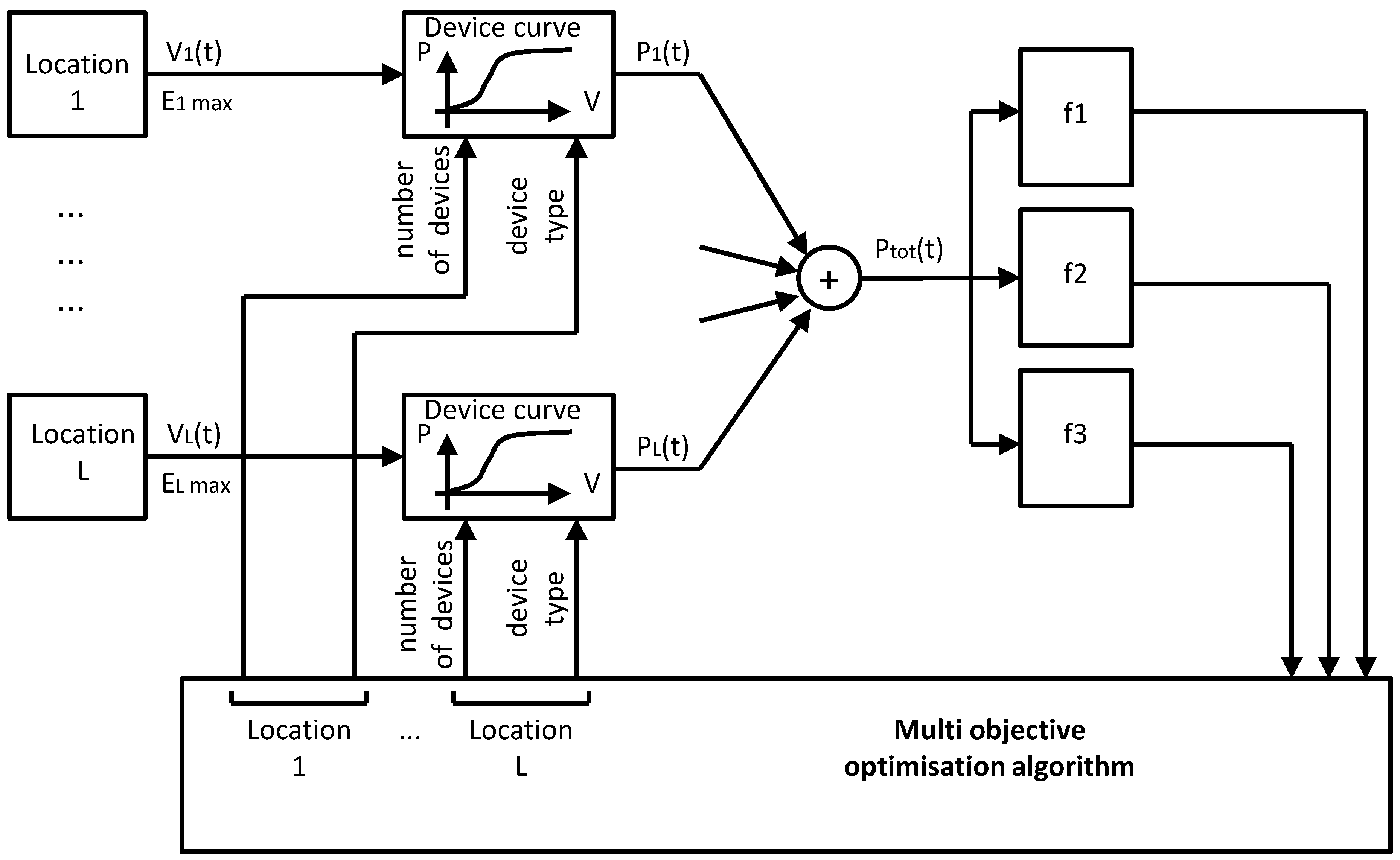
The block diagram of the MOP implemented for the current work is shown in Figure 5. The instantaneous power generated in each location is calculated utilising velocity, maximum extractable energy, number of installed devices and type of installed devices. The total power is calculated and subsequently the values of the objective functions. The multi objective optimisation algorithm utilises the values of the objective functions to change the number and type of installed devices, searching for a better distribution of turbines.
Figure 5.
MOP block diagram.

7. Simulation Results
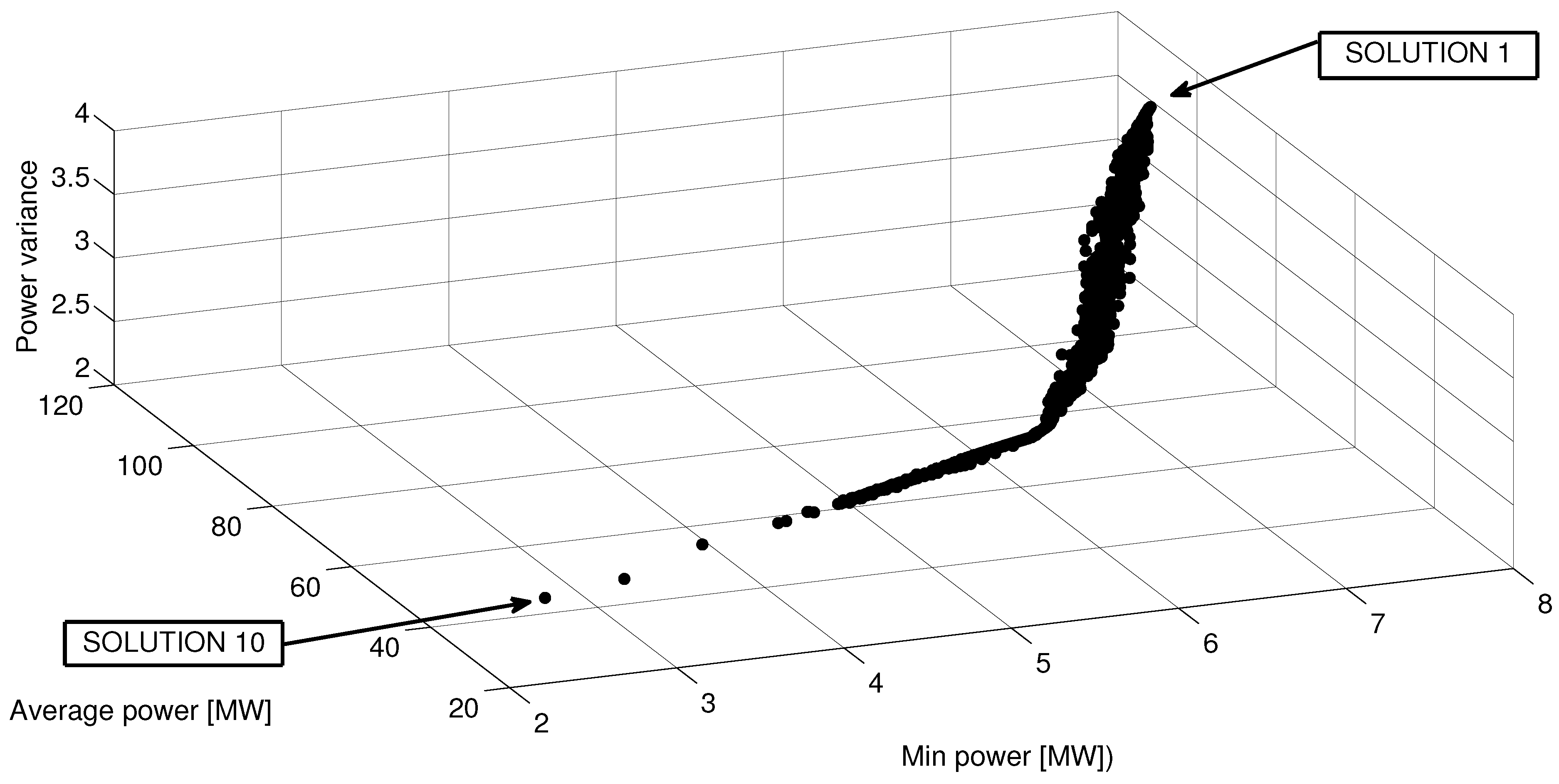
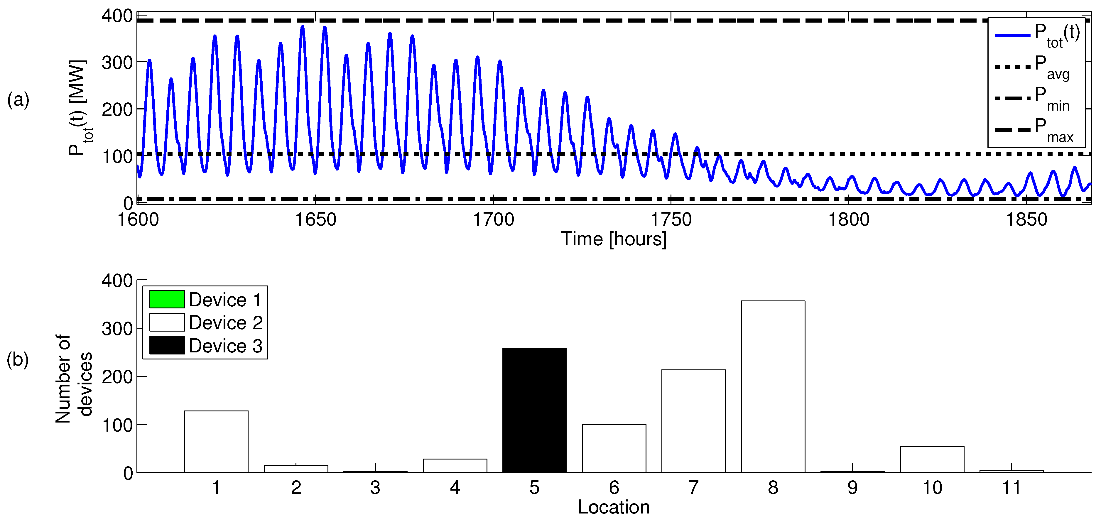
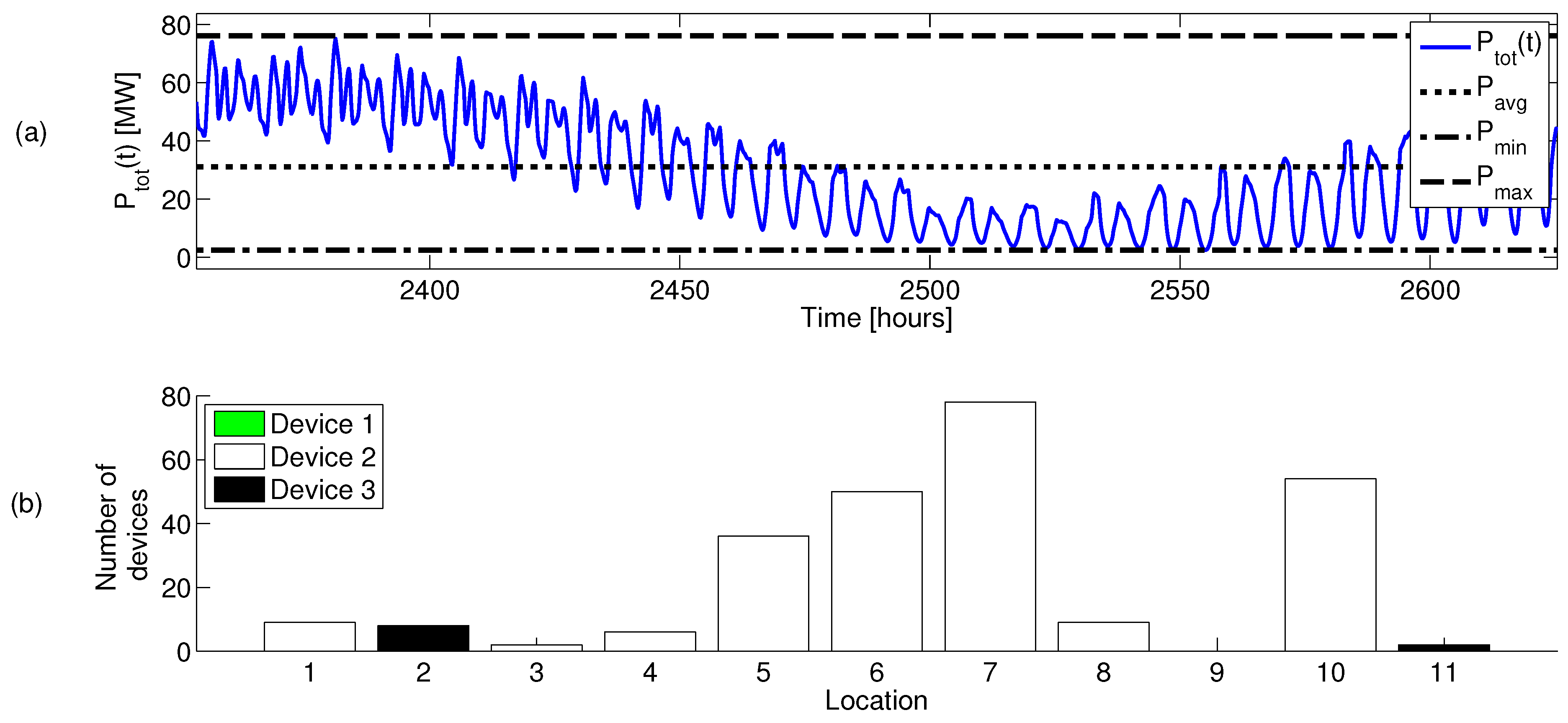
As explained in Section 4.2, in total 11 locations have been utilised to run the simulations: Codling & Arklow Banks, Dursey Sound, Gascanane Sound, Inishtrahull Sound, North East Coast, Ram Race & Copeland Islands, Shannon Estuary, Tuskar Rock & Carnsore Point, Lough Foyle, Strangford Lough and Bulls Mouth. The MOP introduced in Section 6 has been implemented in MATLAB to find the POS and the Pareto front. The utilised MOP solver gamultiobj belongs to the family of genetic algorithms, in particular it is a variation of the NSGA-II algorithms (non-dominated sorting genetic algorithm II) [33,34,35,36]. The result of the simulations is a POS made of 729 different points, each representing a possible configuration of the turbine installations. The corresponding Pareto front is shown in Figure 6. The highest value of the objective function (103.745 MW) is provided by Solution 1; the highest value of the objective function (7.812 MW) is provided by Solution 1 as well and the lowest value of (2.368) is provided by Solution 10 (Table 4). Figure 7a and Figure 8a show different zooms of the time evolution of total power for Solution 1 and 10 respectively. Figure 7b, Figure 8b and Table 5 show the POS for Solution 1 and 10, represented by the number of installed devices and device type. Table 6 shows the extracted energy per year, as a fraction of the viable energy at each location. The main goal of the current paper is to investigate the possibility of creating a minimum constant supply of power to the national electric grid; for this reason, the objective function (related to ) is particularly important. For the purpose of the current work, Solution 1 looks more appropriate than Solution 10. It is interesting to observe that with Solution 10 the number of installed devices is 254, considerably lower than that for Solution 1 (1161 devices). Despite the lower value of energy produced, from an economic point of view, Solution 10 remains an interesting possibility because it provides an appreciable with reduced capital investment compared with solution 1.
Figure 6.
Simulation results: 3D Pareto front.

Figure 7.
Simulation results for Solution 1 (solution with the highest average power and the highest minimum power). (a) Zoom of the total power ; (b) Number of installed devices at each location.
Figure 7.
Simulation results for Solution 1 (solution with the highest average power and the highest minimum power). (a) Zoom of the total power ; (b) Number of installed devices at each location.

Figure 8.
Simulation results for Solution 10 (solution with the lowest power variance). (a) Zoom of the total power ; (b) Number of installed devices at each location.
Figure 8.
Simulation results for Solution 10 (solution with the lowest power variance). (a) Zoom of the total power ; (b) Number of installed devices at each location.

| Objectives | Solution 1 | Solution 10 |
|---|---|---|
| (MW) | 103.745 | 31.126 |
| (MW) | 7.812 | 2.476 |
| 3.667 | 2.368 |
Table 5.
Simulation results: POS (number of installed devices and device type) for the solutions 1 and 10.
| Location | Solution | Solution 10 | ||
|---|---|---|---|---|
| Number of devices | Device type | Number of devices | Device type | |
| 1-Codling & Arklow Banks | 128 | 2 | 9 | 2 |
| 2-Dursey Sound | 15 | 2 | 8 | 3 |
| 3-Gascanane Sound | 2 | 3 | 2 | 2 |
| 4-Inishtrahull Sound | 28 | 2 | 6 | 2 |
| 5-North East Coast | 258 | 3 | 36 | 2 |
| 6-Ram Race & Copeland Islands | 100 | 2 | 50 | 2 |
| 7-Shannon Estuary | 213 | 2 | 78 | 2 |
| 8-Tuskar Rock & Carnsore Point | 356 | 2 | 9 | 2 |
| 9-Lough Foyle | 3 | 3 | 0 | 1 |
| 10-Strangford Lough | 54 | 2 | 54 | 2 |
| 11-Bulls Mouth | 4 | 2 | 2 | 3 |
Table 6.
Simulation results: extracted energy per year at each location, as fraction of the total available energy.
| Location | Solution 5 | Solution 146 |
|---|---|---|
| 1-Codling & Arklow Banks | 99.33% | 6.98% |
| 2-Dursey Sound | 97.04% | 95.55% |
| 3-Gascanane Sound | 98.84% | 53.54% |
| 4-Inishtrahull Sound | 99.34% | 21.29% |
| 5-North East Coast | 99.89% | 7.55% |
| 6-Ram Race & Copeland Islands | 99.51% | 49.76% |
| 7-Shannon Estuary | 99.80% | 36.55% |
| 8-Tuskar Rock & Carnsore Point | 99.98% | 2.53% |
| 9-Lough Foyle | 96.83% | 0.00% |
| 10-Strangford Lough | 98.36% | 98.36% |
| 11-Bulls Mouth | 81.35% | 75.10% |
The POS (and the corresponding Pareto front) provides a spectrum of solutions, and it is the final decision maker who, evaluating the possible trade-offs, has to decide on a final solution. It is important to underline that additional information regarding technologies and installation costs are also critical in evaluating the best final solution.
8. Conclusions
In the current article, a methodology capable of analysing different types of tidal data, such as simulations from hydrodynamic models and tidal stream atlas data, has been developed. Eleven locations have been selected and their velocity and maximum extractable energy have been quantified. Three different turbine curves have been exploited for the simulations. A MOP problem has been set, introducing three objective functions to optimise the total average produced power, the minimum of total average produced power and the variance of total average produced power. The Pareto optimal set of the MOP has been calculated, and in particular, two possible solutions of the found POS have been analysed, calculating for each solution the number and type of installed devices in each location, and providing the corresponding performances and trade-offs. In particular, a specific installation of 1161 devices (Solution 1) provides an interesting = 7.812 MW during the whole year, evidence that it is possible to provide a base load of power to the Irish electric grid utilising the difference of phases of the tidal stream velocity along the Irish coast. Furthermore, Solution 10 provides a base load of = 2.476 MW with the installation of 254 devices. This solution would provide the possibility to install the tidal turbines with a reduced capital investment.
Improvement for future works can be based on the introduction of more accurate data to run the simulations. First of all, more accurate local velocity can guarantee more reliable solutions. The only way to obtain this is to record the local current velocities. Secondly, device curves of real turbines should be utilised, as this would increase the realism of the found solutions (during the current work no published real device curves were available). Finally, to provide a more realistic quantification of the amount of extractable energy in each location, it would be useful to introduce an explicit relationship between the number of installed turbines in a specific location and the reduction of the tidal stream velocity.
Furthermore, the simulations of the current work are done with the hypothesis that the national electric grid is without power loss. In this way the optimisation problem is simplified, but the error introduced is restrained. We expect that the POS and the Pareto front, in case of dispersive electric lines, does not change considerably from the obtained results.
Finally, the developed methodology is totally independent from the specific sea under analysis, and it can be utilised to analyse the potential of other areas around the world, in locations such as Scotland, America or Australia, to verify the possible provision of a base load with tidal stream energy.
Acknowledgements
The authors would like to thank the Irish Marine Institute for providing the tidal current velocities of the locations: Codling & Arklow Banks, Dursey Sound, Gascanane Sound, Inishtrahull Sound, North East Coast, Ram Race & Copeland Islands and Tuskar Rock & Carnsore Point.
Conflict of Interest
The authors declare no conflict of interest.
References
- Elghali, S.B.; Benbouzid, M.; Charpentier, J. Modelling and control of a marine current turbine-driven doubly fed induction generator. IET Renew. Power Gener. 2010, 4, 1–11. [Google Scholar] [CrossRef] [Green Version]
- Kamphuis, W.J. Introduction to Coastal Engineering and Management; World Scientific: Singapore, 2010. [Google Scholar]
- Reeve, D.; Chadwick, A.; Fleming, C. Coastal Engineering: Processes, Theory and Design Practice; Spon Press: Abingdon, UK, 2004. [Google Scholar]
- Hardisty, J. The Analysis of Tidal Stream Power; Wiley: Hoboken, NJ, USA, 2009. [Google Scholar]
- Boon, J.D. Secrets of the Tide, Tide and Tidal Current Analysis and Predictions, Storm Surges and Seal Level Trends; Horwood: Cambridge, UK, 2004. [Google Scholar]
- Pugh, D.T. Tides Surges and Mean Sea Level; John Wiley & Sons: Hoboken, NJ, USA, 1996. [Google Scholar]
- Admiralty. Tidal Stream Atlas NP160, Tidal Harmonic Constants, European Waters, 5th ed.; Hydrographic Office: Taunton, UK, 2009. [Google Scholar]
- Admiralty. Tide Tables NP201-01 Volume 1, United Kingdom and Ireland (including European Channel Ports); Hydrographic of the Navy: Taunton, UK, 1999. [Google Scholar]
- Irish Marine Institute. Available online: http://www.marine.ie/Home/ (accessed on 13 January 2013).
- Wiegel, R.L. Oceanographical Engineering; Dover Publications Inc: New York, NY, USA, 2005. [Google Scholar]
- Forrester, W.D. Canadian Tidal Manual; Government of Canada Fisheries and Oceans: Ottawa, Canada, 1983.
- Sustainable Energy Ireland (SEI). Tidal & Current Energy Resources in Ireland; Technical Report; Sustainable Energy Ireland: Dublin, Ireland, 2006. [Google Scholar]
- Admiralty. Tidal Stream Atlas NP 222, Firth of Clyde and Approaches, 1st ed.Hydrographic Office: Taunton, UK, 2003.
- Admiralty. Tidal Stream Atlas NP 256, Irish sea and Bristol Channel, 4th ed.Hydrographic Office: Taunton, UK, 2006.
- Marina Guide Dover 2012; Dover Marina: Dover, UK, 2012.
- AquaFact. ADCP deployments at Achill Island and Shannon Estuary June-July 2004 (Tidal & Current Energy Resources in Ireland, Appendix A); Technical Report; Sustainable Energy Ireland: Dublin, Ireland, 2006. [Google Scholar]
- Sustainable Energy Ireland (SEI). Site Locations and Conservation Areas (Tidal & Current Energy Resources in Ireland, Appendix D); Technical Report; Sustainable Energy Ireland: Dublin, Ireland, 2006. [Google Scholar]
- Kean, N. Sailing Directions for the East and North Coasts of Ireland; Irish Cruising Club: Ireland, 1999. [Google Scholar]
- Kean, N. Sailing Directions for the South and West Coasts of Ireland; Irish Cruising Club: Ireland, 2008. [Google Scholar]
- Rainsbury, D. Irish Sea Pilot; Imray: St Ives, England, UK, 2009. [Google Scholar]
- Garrett, C.; Cummins, P. Limits to tidal current power. Renew. Energy 2008, 33, 2485–2490. [Google Scholar] [CrossRef]
- Sustainable Energy Ireland (SEI). Tidal & Current Energy Resources in Ireland (APPENDIX E); Technical Report; Sustainable Energy Ireland: Dublin, Ireland, 2006. [Google Scholar]
- Irish Marine Institute—Model Validation. Available online: www.marine.ie/home/services/ operational/oceanography/ModelValidation (accessed on 21 January 2013).
- Fernandes, A.; Das, V.K.; Bahulayan, N. Harmonica tidal analysis at a few stations using the least squares method. Mahasagar 1991, 24, 1–12. [Google Scholar]
- Boon, J.D.; Kiley, K.P. Harmonic Analysis and Tidal Prediction by the Method of Least Squares; Special Report No. 186; Virginia Institute of Marine Science: Gloucester Point, VA, USA, 1978. [Google Scholar]
- Chapra, S.C. Applied Numerical Methods with Matlab for Engineers and Scientists, 3rd ed.; McGraw Hill: New York, NY, USA, 2011. [Google Scholar]
- MathWorks. Least-Squares Fitting. Available online: http://www.mathworks.co.uk/index.html (accessed on 5 January 2013).
- Holmes, P. Professional Development Programme: Coastal Infrastructure Design, Construction and Maintenance. A Course in Coastal Defence System I, Chapter 4, Coastal Processes: Tides and Tidal Flows; Technical Report; University of the West Indies: Mona, Jamaica, 2001. [Google Scholar]
- Giorgi, S. Can Tidal Currents Energy Provide Base Load? Master’s thesis, National University of Ireland, Maynooth (NUIM), Maynooth, Ireland, 2012. [Google Scholar]
- Fraenkel, P.L. Power from marine currents. Proc. Inst. Mech. Eng. A 2002, 216, 1–14. [Google Scholar] [CrossRef]
- Blunden, L.S.; Bahaj, A.S. Tidal energy resource assessment for tidal stream generators. Proc. Inst. Mech. Eng. A 2007, 221, 137–146. [Google Scholar] [CrossRef]
- Benelghali, S. On Multiphysics Modeling and Control of Marine Current Turbine Systems. Ph.D. Thesis, Université Européenne de Bretagne, Rennes, France, 2010. [Google Scholar]
- Konak, A.; Coit, D.W.; Smith, A.E. Multi-objective optimization using genetic algorithms: A tutorial. Reliab. Eng. Syst. Saf. 2006, 91, 992–1007. [Google Scholar] [CrossRef]
- Arora, J.S. Introduction to Optimum Design; Academic Press: San Diego, VA, USA, 2004. [Google Scholar]
- Goldberg, D.E. Genetic Algorithms in Search, Optimization and Machine Learning; Addison-Wesley: Boston, MA, USA, 1989. [Google Scholar]
- Osyczka, A. Evolutionary Algorithms for Single and Multicriteria Design Optimization; Physica-Verlag: Heidelberg, Germany, 2002. [Google Scholar]
© 2013 by the author; licensee MDPI, Basel, Switzerland. This article is an open access article distributed under the terms and conditions of the Creative Commons Attribution license (http://creativecommons.org/licenses/by/3.0/).
Share and Cite
MDPI and ACS Style
Giorgi, S.; Ringwood, J.V. Can Tidal Current Energy Provide Base Load? Energies 2013, 6, 2840-2858. https://doi.org/10.3390/en6062840
AMA Style
Giorgi S, Ringwood JV. Can Tidal Current Energy Provide Base Load? Energies. 2013; 6(6):2840-2858. https://doi.org/10.3390/en6062840
Chicago/Turabian StyleGiorgi, Simone, and John V. Ringwood. 2013. "Can Tidal Current Energy Provide Base Load?" Energies 6, no. 6: 2840-2858. https://doi.org/10.3390/en6062840