Assessing Tolerance-Based Robust Short-Term Load Forecasting in Buildings

Abstract

Short-term load forecasting (STLF) in buildings differs from its broader counterpart in that the load to be predicted does not seem to be stationary, seasonal and regular but, on the contrary, it may be subject to sudden changes and variations on its consumption behaviour. Classical STLF methods do not react fast enough to these perturbations (i.e., they are not robust) and the literature on building STLF has not yet explored this area. Hereby, we evaluate a well-known post-processing method (Learning Window Reinitialization) applied to two broadly-used STLF algorithms (Autoregressive Model and Support Vector Machines) in buildings to check their adaptability and robustness. We have tested the proposed method with real-world data and our results state that this methodology is especially suited for buildings with non-regular consumption profiles, as classical STLF methods are enough to model regular-profiled ones.

1. Introduction

Load forecasting is an essential part of the scheduling, management and operation of a power system. Since electrical energy cannot be stored, it is important to deliver an accurate prediction in order to avoid dispatch problems due to unexpected loads. Moreover, energy market stakeholders also require trustworthy information in order to be more competitive when purchasing electricity. In addition, the use of the data recorded in smart-meters and software tools may help prevent demand peaks in a reliable and efficient fashion.

Short-term load forecasting (STLF) is the prediction of energy demand in a time-span ranging from minutes to several days, being crucial for several smart grid applications. As discussed above, it is important for the economic and secure operation of power grids, but several factors should be considered as well. For instance, the publication of the energy consumption and its conversion to equivalent CO${}_2$ emissions decreases the load that affects future predictions due to its influence on social consciousness. Moreover, it also helps the energy retailer in order to negotiate a better price. In the end, an accurate forecast results in higher savings while helping to maintain the security of the grid.

There exists a large bibliography on STLF (see [1,2,3] for a comprehensive survey). Most of the methods used can be divided into two main groups depending on the strategy followed: Statistical Methods, which estimate the present value of a given variable depending on the values in the past (i.e., consumption records [2,4,5]), and Artificial Intelligence methods, which have been applied successfully to a wide variety of real-world applications, demonstrating their ability to learn the relationships between input and output variables. Moreover, the later have been proven to be ideal when dealing with risk and uncertainty (the main aspects behind prediction). This approach, however, involves the need of an expert whose knowledge can be incorporated into the system capable of making accurate forecasts. The most popular algorithms, according to their efficiency, are Support Vector Machines (SVM) [6,7] and Neural Networks (NN) [8,9]. Note that in this paper we will only use SVM since we have not been able to replicate the results from the literature involving NNs. Moreover, our tests have proven that NNs are slower and do not obtain better results than other techniques (see for example [10]).

Despite the accuracy they provide on forecasting, Artificial Intelligence methods suffer from a great number of disadvantages such as difficult parametrisation, non-obvious selection of variables and the requirement of more historical data to learn than any of the Statistical Methods [2]. Furthermore, they rely on a tedious trial-and-error process to tune them up properly.

This paper focuses on building STLF, a particular case dealing with issuing day-ahead energy consumption predictions in non-residential buildings such as schools, universities, public buildings or companies’ facilities. The ideal to reach is the so-called zero energy building, (i.e., any construction presenting annually zero net energy consumption and carbon emissions), and, with this objective in mind, there are a number of technologies that must be integrated:

• Weatherproofing, insulation and automatic HVAC (heating, ventilation, and air conditioning).
• Energy re-utilisation (as in co- or tri-generation).
• Use of renewable energy sources and energy storage systems.
• Demand response controllers attached to the HVAC and other loads.

Clearly, STLF is crucial in the last two points. Indeed, maximising the efficiency of the demand response controller requires an accurate forecast for both energy consumption and energy generation (as well as a reliable storage controller).

This branch presents different features. For instance, in normal country-wide STLF, the non-linearity of the load becomes smoothed: expected consumption that does not take place is compensated by non-expected consumption that does (i.e., the consumption curve tends to be seasonal and regular). In contrast, the load profile of a building is more chaotic coinciding with the times it is used. Hence, there is no consumption at night (or it is negligible) and there exists a notable difference between idle and active times. Furthermore, some of these buildings are not yet fully-automated: either the HVAC is manually controlled or it is switched on and off remotely, issues that affect greatly on energy consumption. Another critical aspect is that there is usually scarce (if any) historical data on hourly load and the load profile is sure to vary and evolve over time (just think of the gadgets an office used to have ten years ago compared with nowadays fully-equipped on-line ones). This makes it very difficult to extract the trend component and/or use forecasting methods that need long learning windows (such as ARIMA and their derivatives).

While operating in real environment, it is vital that the forecasting method adapts to changing conditions. If the system cannot react to these changes, the predictions obtained from the system will fail. In order to achieve an optimal prediction, we need a method that evolves over time and is not subject to fixed laws so as to conform to recent data. This is the reason that explains why some models present very good records in a certain situation but fail in others. Meta-learning models address this issue: they belong to a well-established procedure for improving forecasting accuracy [11] and have already been applied in other disciplines (see [12] for a broad survey).

Analysing the buildings’ electricity consumption series, we can observe the presence of atypical values that digress from the typical model. They significantly degrade the accuracy of conventional day-ahead estimation even if they appear in a reduced number. These atypical values present two natures:

• New Pattern: Some days show a different consumption pattern due to reasons of diverse nature (e.g., long weekends, sport events, election polls, strikes, etc.). In the end, the load of these days consists of a new day-type on its own (see Section 3 for more details) and it should be removed from the learning set or classified beforehand.
• Scaled Pattern: On the other hand, some days follow profiles similar to those from existing day-types but scaled down or up. Again, these changes can be due to diverse causes (e.g., sudden weather changes, long weekends, special events, works, etc.). The load in these days does not consist of a new day-type but can be just an extreme statistical fluctuation or simply represent an underline change in the building (such as new equipment) that may be extended along the time. In the first case, there should be no action, but in the second one, the learning window should be restarted.

Thus, the data series should be treated in a robust way, namely, the forecasting method should recognise these atypical values and treat them accordingly in order to avoid burst errors that worsen the overall forecast.

Against this background, we present here a comparison of several robust methods based on threshold values over the errors. We aim at assessing them in order to evaluate whether they can correctly distinguish between the two types of anomalies explained above and fulfil the premises required by a robust algorithm.

The remainder of the paper is organised as follows. Section 2 discusses the related work. Section 3 presents the different algorithms used in the prediction, the features of the used datasets, an explanation of the method and its validation. Section 4 describes the datasets used. Section 5 details the tests and comments the obtained results. Finally, Section 6 summarises our contribution and draws the avenues of future works.

2. Related Work

As previously mentioned, there exists a remarkable work on STLF but, comparatively, not so much related to buildings and the use of meta-learning to provide an appropriate solution in this scope. We have previously researched on this field [13]. Nevertheless, it was not focused on the robustness of the prediction but on the evaluation of model combination and other model-selection methods.

STLF in buildings provides a whole new overview on the paradigm, giving way to several important works such as using a SVM to predict the load of a building complex [14,15], where a NN is tuned up by Automatic Relevance Determination in order to optimise the selected input. In addition, [8] used the temperature data in a feedback NN obtaining a remarkable Mean Absolute Percentage Error (MAPE) of 1.945% (Section 4.3 details the mathematical definition of this type of error measure), but this result was obtained measuring only a single week in a whole year, which is not statistically representative. Finally, all artificial intelligence methods waste most of their efforts in modelling non-linear behaviour of the work calendar [16,17].

In the case of meta-models for normal STLF, research has taken two main directions. The first uses a meta-heuristic to calculate the best set of parameters of a SVM or a NN [18,19,20], but these works suffer from the same flaw in the single models. The second area has explored the optimal way of combining the output of the single models, usually by assigning weights (see [21] for different approaches to this end). For instance, a very simple but effective approach consists in defining equal weights, which has shown to be surprisingly effective [22,23]. More sophisticated approaches include linear combination [24], dynamic optimal weight combination [25], a genetic algorithm as best model selector [26] or rule-based best model selection [27].

Assessing the robustness of STLF has received very little attention [9,28] and all the efforts focus on the detection of outliers (new patterns of atypical values in our nomenclature) in the time series of national loads.

3. Adaptive STLF in Buildings

3.1. Overall Methodology

In order to ensure the required standard of security and quality in a power system, we need a very reliable and robust forecast. This paper focuses on assessing an adaptive forecasting that tries to mimic the consumption behaviour. Since all methods need a learning period of time, new consumption habits lead to prediction inaccuracies that increase both economic and technical costs.

In this work, we have used the following methodology; we repeat the next steps for every day in the dataset except for the first day of every day-type. Figure 1 shows a sequence diagram of the methodology. Please note that the meter is virtually connected to a real-time processing network as described in [29], to which we will refer from now on as the Platform.

Figure 1. Sequence diagram of the proposed methodology.

Figure 1. Sequence diagram of the proposed methodology.

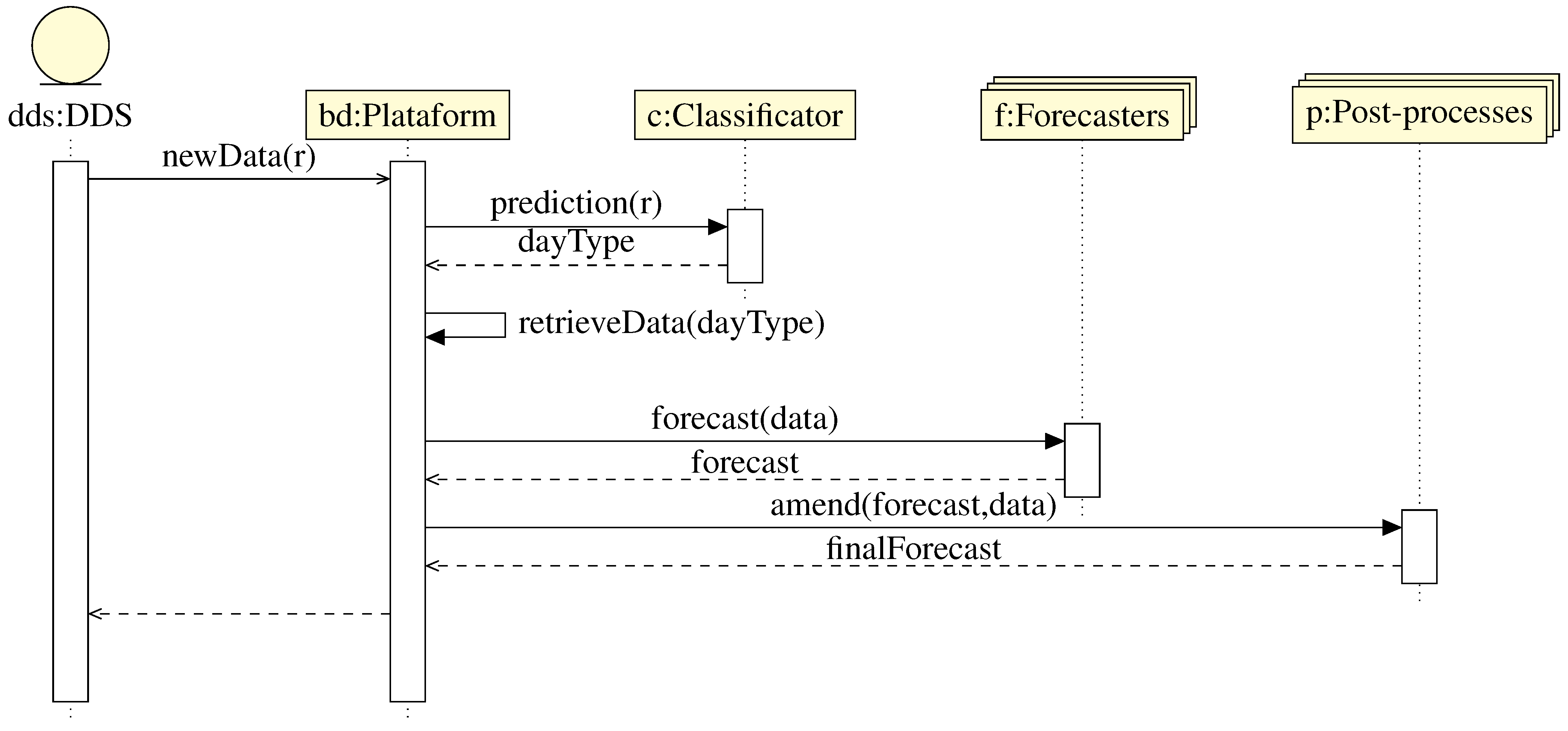
• Data Distribution Service (DDS): A meter sends a new measure to the Platform through the DDS bus. This measure is stored to then be used to issue a forecast.
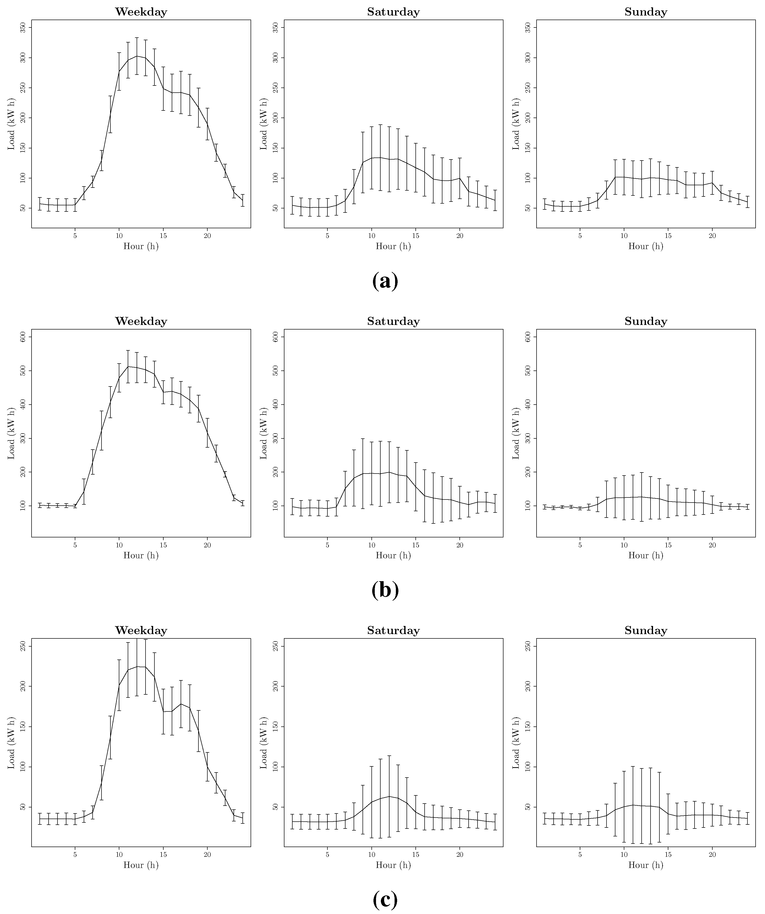
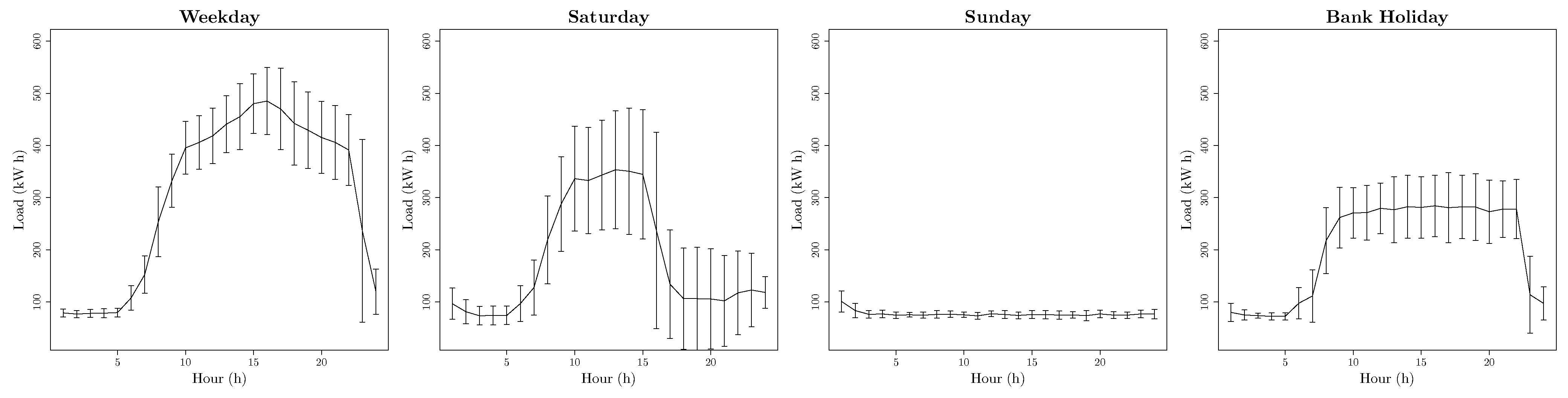
• Classificator: In this step, the Platform sends the new data to the Classificator and queries it for the prediction of the day-type for the next day. In previous works [30], we have compared several clustering techniques with the use of the local work calendar. Our results conclude that the best option is to use the work calendar if it is available. Hence, buildings may present different number of day-types. Specifically, in our tests, there are buildings presenting:

  -

  Two day-types: (Weekday and Weekends) such as $c59$ or $ashrae$ (see Section 4 for more information on the datasets). This building is characterised by the lack of consumption on Saturdays. An example of this behaviour can be seen in Figure 2.

  -

  Three day-types: (Weekday, Saturdays and Sundays) such as the four $donosti$ datasets, $bilba{o}_1$, $bilba{o}_3$ or $bilba{o}_4$. They present a very similar consumption to commercial or service buildings. An example of this behaviour can be seen in Figure 3 and Figure 4.

  -

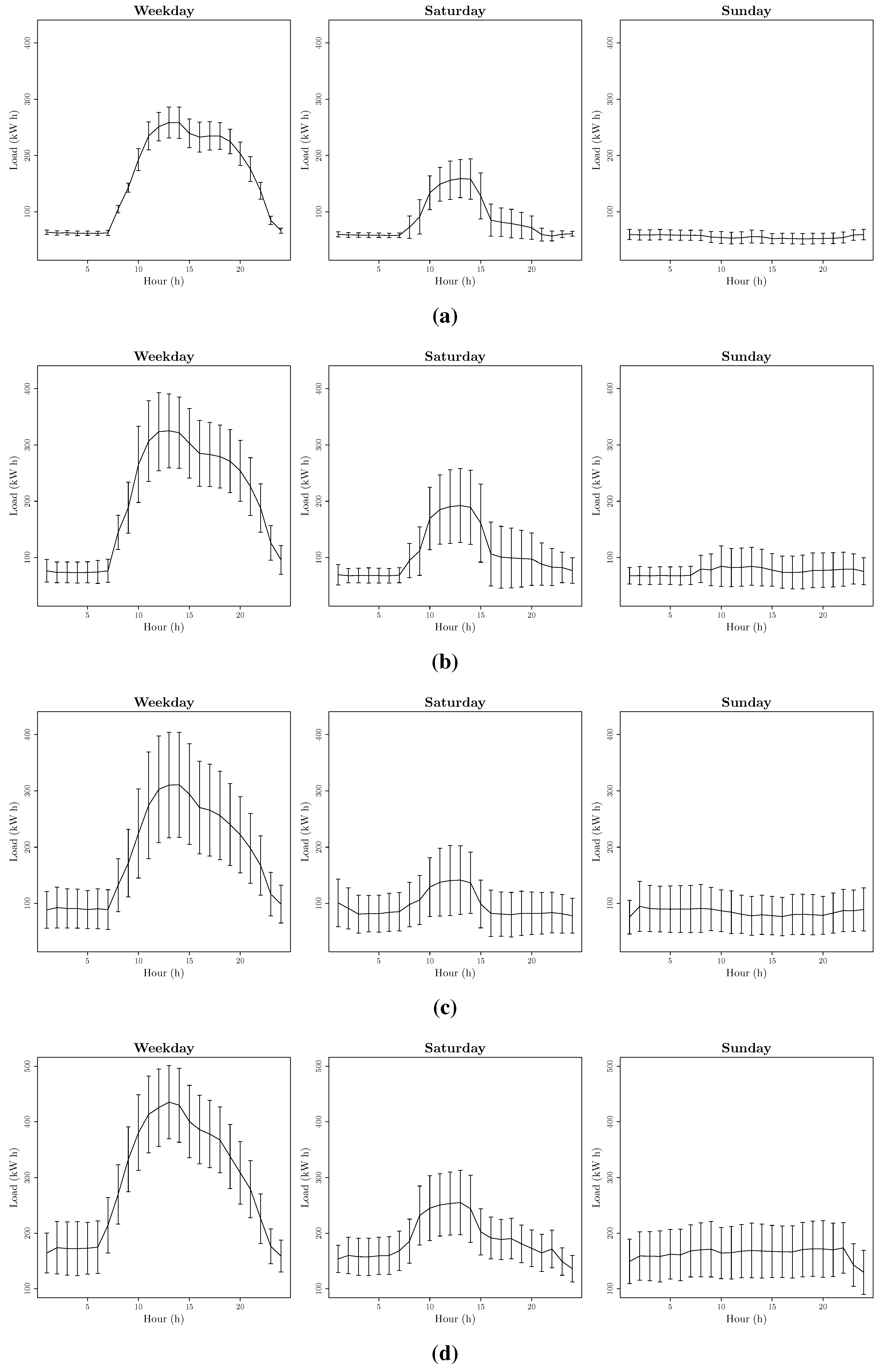
  Four day-types: (Weekday, Saturdays, Sundays and Bank Holidays) such as $bilba{o}_2$. This building shows a special behaviour in Bank Holidays. In Figure 5 can be seen an example of this behaviour.

• Forecasters: In the next step, the Platform sends the data of the previous days of the same day-type to the Forecasters. They will adjust the model parameters and then issue a forecast. Note that we have a different model for every day-type, and therefore we must re-train the model for every day.

In this work, we have used AR and SVM models, since according to our experiments [10,30] they produce the best results using this methodology. Moreover, in these works we have optimised the free parameters by means of a grid search following the advice given in [31] and we used the results of these test here.

Figure 2. Typical load for the dataset with two day-types. Average daily load ($\mathrm{kW}\mathrm{h}$). Error bars denotes $\pm \sigma$. (a) Dataset $c59$; (b) Dataset $ashrae$.

Figure 2. Typical load for the dataset with two day-types. Average daily load ($\mathrm{kW}\mathrm{h}$). Error bars denotes $\pm \sigma$. (a) Dataset $c59$; (b) Dataset $ashrae$.

• Post-processes: Finally, in this stage the Platform sends the forecasts issued by the forecasters to the post-processes in order to improve the results. Examples post-process are:

  -

  Bias Correction: some models produce forecast that are systematically biased. We can measure that bias and compensate it. In [10] we have assessed the performance of this post-process.

  -

  Model Selection: some models issue a more reliable forecast at certain hours or day-types than others. In [13], we presented a comparison of different strategies to select the best model in every moment.

  -

  Model Combination: another option is to group all the predictions issued by the forecasters in order to build a more robust forecast. We have addressed this strategy in [13,32].

Please note that in this work we have not used these three post-processes as we have assessed their performance in previous works. In Section 3.2 we will present two more examples of post-processes that we will analyse in this paper.

Figure 3. Typical load for the dataset with three day-types. Average daily load ($\mathrm{kW}\mathrm{h}$). Error bars denotes $\pm \sigma$. (a) Dataset $donost{i}_1$; (b) Dataset $donost{i}_2$; (c) Dataset $donost{i}_3$; (d) Dataset $donost{i}_4$.

Figure 3. Typical load for the dataset with three day-types. Average daily load ($\mathrm{kW}\mathrm{h}$). Error bars denotes $\pm \sigma$. (a) Dataset $donost{i}_1$; (b) Dataset $donost{i}_2$; (c) Dataset $donost{i}_3$; (d) Dataset $donost{i}_4$.

Figure 4. Typical load for the dataset with three day-types. Average daily load ($\mathrm{kW}\mathrm{h}$). Error bars denotes $\pm \sigma$. (a) Dataset $bilba{o}_1$; (b) Dataset $bilba{o}_3$; (c) Dataset $bilba{o}_4$.

Figure 4. Typical load for the dataset with three day-types. Average daily load ($\mathrm{kW}\mathrm{h}$). Error bars denotes $\pm \sigma$. (a) Dataset $bilba{o}_1$; (b) Dataset $bilba{o}_3$; (c) Dataset $bilba{o}_4$.

Figure 5. Typical load for the dataset with four day-types. Average daily load ($\mathrm{kW}\mathrm{h}$). Error bars denotes $\pm \sigma$. Dataset $bilba{o}_2$.

Figure 5. Typical load for the dataset with four day-types. Average daily load ($\mathrm{kW}\mathrm{h}$). Error bars denotes $\pm \sigma$. Dataset $bilba{o}_2$.

3.2. Proposed Post-Process Methods

Despite all the post-process methods, we have detected that some days in the datasets are very different from what their normal profile should be according to their day-type. This abnormal behaviour causes burst errors to appear in the forecast until the algorithms manage to adapt to these changes. Thus, we need a faster method in order to avoid large errors in such days.

In this paper, we introduce two post-process methods that check whether the prediction error is bigger than a given threshold value k. Please note that we can use whatever error we define provided that the threshold value is in the same units as the error. As in this paper we are using MAPE error (see Section 4.3 for details), k should be a percentage. Moreover, this value can be fixed a priori or have an adaptive value like:

$$k:=\sqrt{\frac{c}{24q}\sum _{d\in Q}\sum _{h=1}^{24}{(e_{d,h}-\widehat{e})}^2}$$

(1)

where Q denotes the set of days in the learning window at that moment, q is the number of days in the learning window, $e_{d,h}$ denotes the residuals of the model in day d and hour h and $\widehat{e}$ denotes the mean error of the model in the entire learning window. Note that this value is just the variance of the residuals multiplied by the fixed constant c. Please note that this value should be tailored specifically to every dataset. In this work we have made a grid search for this value and found that the best option is $c:=3$.

In case the error in one day is above the threshold value k, one of the two post-processes acts.

• Learning Window Re-Initialization: In this case, we reboot the learning windows in order to avoid anomalies of the scaled pattern type (i.e., we completely delete the data in the dataset and replace it with the newest value). Since the learning windows are very short (just three days in this test, see [10,13] for a broad comparison in this matter) and the models used are sufficiently robust to tailor this degenerated training set, we are able to issue a new forecast in this situation. Moreover, the forecast produced is the obvious one, just the values observed the previous day (i.e., acts like a Random Walk Model), so this adjustment quickly adapts to changes in the dataset.
• Skipping Anomalies: In this case we avoid introducing the new pattern in the training data in order to avoid anomalies of the new pattern type.

Note that we have not used both methods simultaneously. Moreover, we only present here the results of the Learning Windows Re-Initialization method without using the adaptive threshold value, as both the Skipping Anomalies and the Adaptive Threshold Methods produce much worse results (in any combination).

3.3. Forecasting Models

All models used can be classified as regression models. Namely, they follow the equation:

$$LOAD\left(h\right):=f\left(h\right)+\epsilon$$

(2)

where $h\in [0,23)$ denotes time, $LOAD\left(h\right)$ denotes the load at time h, f is the model used and ε is a random variable.

3.3.1. Time Series Model

The first model is an Autoregressive Model commonly used for modelling univariate time series. For every day-type d we have:

$$s^d\left(h\right)=\sum _{i=1}^q{\phi }_i^d{r}^d(h,i)$$

(3)

where ${\phi }^d:=({\phi }_1^d,\dots ,{\phi }_q^d)$ are the model parameters and $r^d(h,i)$ denote the real load measured at time h of the i-th previous day of day-type d. Namely, in the adjusting step, we have retrieved the q last values of the same day type (e.g., with $q=3$, from a Tuesday, the previous Monday, Friday, Thursday) and not the q last chronological values (e.g., from a Tuesday, the previous Monday, Sunday, and Saturday) and then we have made a convex combination with the model coefficients ${\phi }^d$. In order to give a higher priority to the latest data against the oldest values, the model coefficients are drawn by a polynomial or an exponential method. The polynomial method produces the following parameters

$${\phi }_i=\frac{{(q-i)}^l}{{\sum }_{i=0}^q{(q-i)}^l}$$

(4)

whereas the exponential method produces

$${\phi }_i=\frac{l^{(q-i)}}{{\sum }_{i=0}^q{l}^{(q-i)}}$$

(5)

where q is the length of learning window and l can take integer values. In this work, we has chosen the exponential method with parameter $l:=2$. This value has been taken based on empirical experience. Please note that, with this nomenclature, we have fixed the number of learning days to $q:=3$ as previously stated.

3.3.2. Support Vector Machines Model

A SVM constructs a hyperplane, or a set of hyperplanes, in a high or infinite dimensional space, which can be used for classification or regression. SVMs have been previously used for load forecasting in buildings [14]. Here, we have used a ν-SVR. Note that, as we have explained before in Equation (2), the function we regress is the load curve of all day taking only the time as input. As in the previous case, we take a model for every day-type and train every model with the last q days of the same type. The rest of the free parameters are: radial basis function as kernel, threshold $\nu :=0.9$, soft margin parameter $C:=10$ and kernel parameter $\gamma :=1$. The explanation of these parameters is out of the scope of this paper; we encourage the reader to see [33] for an in-depth explanation.

4. Datasets

This study comprises several datasets in order to provide the most representative result possible: ten datasets from seven different buildings’ consumption data records and five from Transmission System Operators (TSO) records from different countries. Table 1 and Table 2 summarise the main characteristics of these datasets. These tables also contain an estimation of the expected value of the error for every dataset under the hypothesis that ε follows a Gaussian Random Variable (column Expected MAPE), which according to our experiments is a fair assumption. Please note that in [32] we present a detailed description of the estimation process. Moreover, some TSOs publish their own STLF so we can calculate their error in the same way as with our predictions. Column MAPE from Operator of Table 2 contains this value.

Table 1. Summary of the buildings’ features. N/A denotes unknown values.

Building	HVAC	Number of day-types	Expected MAPE (%)
$donost{i}_1$	NO	3	6.01
$donost{i}_2$	NO	3	8.22
$donost{i}_3$	YES	3	13.60
$donost{i}_4$	YES	3	8.74
$bilba{o}_1$	NO	3	5.89
$bilba{o}_2$	YES	4	7.22
$bilba{o}_3$	Partially	3	4.82
$bilba{o}_4$	NO	3	5.95
$ashrae$	N/A	2	4.98
$c59$	N/A	2	3.74

Table 1. Summary of the buildings’ features. N/A denotes unknown values.

Building	HVAC	Number of day-types	Expected MAPE (%)
$donost{i}_1$	NO	3	6.01
$donost{i}_2$	NO	3	8.22
$donost{i}_3$	YES	3	13.60
$donost{i}_4$	YES	3	8.74
$bilba{o}_1$	NO	3	5.89
$bilba{o}_2$	YES	4	7.22
$bilba{o}_3$	Partially	3	4.82
$bilba{o}_4$	NO	3	5.95
$ashrae$	N/A	2	4.98
$c59$	N/A	2	3.74

Table 2. Summary of the region’s features. N/A denotes no available values. Note that TSOs use forecasting models especially tailored to their respective consumption profiles.

Region	Expected MAPE (%)	MAPE from Operator (%)
$REE$	5.87	1.08
$EUNITE$	9.20	N/A
$AP$	7.45	5.02
$NYC$	6.95	1.64
$NORTH$	2.04	3.57

Table 2. Summary of the region’s features. N/A denotes no available values. Note that TSOs use forecasting models especially tailored to their respective consumption profiles.

Region	Expected MAPE (%)	MAPE from Operator (%)
$REE$	5.87	1.08
$EUNITE$	9.20	N/A
$AP$	7.45	5.02
$NYC$	6.95	1.64
$NORTH$	2.04	3.57

4.1. Buildings

4.1.1. University of Deusto

We have recorded the energy consumption of several buildings of the University of Deusto in both of its campuses: Donostia-San Sebastián and Bilbao (Basque Country). We have downloaded these data directly from the meter, placed by the Spanish law (54-1997) directly at the transformer, using the IEC 60870-5-102 standard protocol [34].

These buildings present different patterns as each one has its own special features. For example, we have measurements from the Donostia-San Sebastián building complex since March 2009 but it presents three different periods. From March to September, there was only one building with a regular and homogeneous consumption since (among other things) its heating system is not regulated according to the weather: from autumn to spring, it is manually turned on every day at approximately the same time and it works until the building closes at night; therefore, meteorological conditions do not show notable influence on the electricity consumption (season, on the contrary, does) or it is somehow dissolved in the data. These data forms the dataset $donost{i}_1$.

On July 2009, the construction of two more buildings started but this event did not have an impact on the load profile until September 2009 due to the summer holidays. As the behaviour of these three building together are essentially different (a lot more noisy), we have split the dataset and created the $donost{i}_2$ dataset.

Finally, we created the third and fourth dataset ($donost{i}_3$ and $donost{i}_4$) with the rest of the data. Both datasets present the same characteristics but there is a big gap in the records since the utility changed the meter from a GSM based one to an IP based one. The new buildings have an HVAC system for cooling so weather changes might influence the consumption, explaining in this way the high spikes in their loads; however our previous experiments do not show any relationship [30]. The $donost{i}_3$ dataset has a length of 12 months (September 2010–September 2011) while the $donost{i}_4$ dataset has a length of 8 months (April 2012–January 2013)

All builds show quite a regular profile in working days with consumption from 7:00 a.m. to 10:00 p.m. (opening hours go from 8:00 a.m. to 9:00 p.m.). On Saturdays, it shows a peak at noon and on Sundays it is almost flat.

On the other hand, we have also measured the electrical consumptions from four different buildings in the Bilbao Campus of the University of Deusto from September 2012 to January 2013. Three of them, $bilba{o}_1$, $bilba{o}_3$ and $bilba{o}_4$, gather the records from standard university buildings (i.e., classrooms and offices), while $bilba{o}_2$ contains the data of the campus main library. It presents a more hectic activity until late at night as well as during Saturdays and this fact is reflected in the load profile. The rest of the buildings present a similar profile as the ones in the Donostia Campus.

4.1.2. Ashrae competition

The Ashrae competition ([35] dataset $ashrae$ in Figure 2b) comes from an unknown building; the data present a quite similar profile as the dataset $donost{i}_1$ and has a length of only 6 months (September 1989 to February 1990) with consumption from 9 a.m. to 9 p.m.

4.1.3. Casaccia Research Centre

Dataset $c59$ contains the consumptions records from the C59 Building in the Casaccia Research Centre, Rome, Italy, during the months of September to November 2009 [36]. As with the ASHRAE competition data, no information has been provided about the building but the profile is also quite similar to the $donost{i}_1$ dataset, except that there is no consumption on Saturdays.

4.2. Regions

We have also downloaded public data from several TSO in order to contrast whether this post-process methodology works well when forecasting large regions. We have taken the information from:

• $REE$: the Spanish TSO [37], from January 2007 until October 2011.
• $AP$: the Pennsylvania, Jersey, and Maryland Interconnection (PJM) [38], more accurately from the Allegheny Power (AP) zone, from November 2008 until December 2010.
• $NYC$ and $NORTH$: the New York Independent System Operator (NYISO) [39], more accurately from the NYC and NORTH substations. The former contains data from February 2005 until October 2011, the latter from June 2001 to October 2011.
• $EUNITE$: from the Eastern Slovakian TSO (Eunite competition dataset [40]), from January 1997 to December 1998.

As it can be seen in Figure 6, these datasets are essentially different from those of the buildings; they present homoscedasticity and only have two slightly-different patterns: one for weekdays and another for holidays. Table 2 presents a summary of the regions’ characteristics.

Figure 6. Average daily load ($\mathrm{kW}\mathrm{h}$). Error bars denotes $\pm \sigma$. (a) Dataset $REE$; (b) Dataset $AP$; (c) Dataset $NYC$; (d) Dataset $NORTH$; (e) Dataset $EUNITE$.

Figure 6. Average daily load ($\mathrm{kW}\mathrm{h}$). Error bars denotes $\pm \sigma$. (a) Dataset $REE$; (b) Dataset $AP$; (c) Dataset $NYC$; (d) Dataset $NORTH$; (e) Dataset $EUNITE$.

4.3. Test-Bed and Validation Measurements

In this study, we have tailored the Leave-One-Out Cross-Validation (LOOCV) procedure [41] that tries to mimic the performance in real conditions. In this spirit, for each day in the dataset we have issued a prediction using the last q days’ values. Normally, this method cannot be used for the first q days of every day-type but, as we have explained in Section 3, we can already forecast with only one training day.

We use MAPE as error measurement to evaluate performance of the models since it is unit free, which allows comparisons between forecasting errors from different measurement units. Moreover, it is the error measurement most widely used in forecasting despite their problems (see [42] and references therein for an extensive discussion and several solutions to these problems). It is calculated as follows:

$$\mathrm{MAPE}:=\frac{1}{days}\sum _{i=1}^{days}\left(\frac{1}{24}\sum _{h=1}^{24}\frac{\left|r\right(h,i)-p(h,i\left)\right|}{r(h,i)}\right)\times 100$$

(6)

where $p(h,i)$ is the predicted value of the load for the hour h of the day i, $r(h,i)$ refers to the real value and $days$ represents the amounts of days in that particular datasets.

Regarding the validation of the post-process, we follow two steps to check the performance of the method. First, we validate the dataset computing the MAPE committed in the whole dataset. The robust method is compared with the normal one in order to assess which one works better over time. Second, we take a closer view by measuring the errors only in the days where the post-process has worked.

5. Experimental Results

The experiments have been carried out on a Core i7 2600 CPU with 16 GB RAM and a Gentoo Linux up-to-date. The AR model has been implemented by means of a home-made java class, whereas the SVM model uses the libSVM library [43].

Please note that this format has been chosen to assess the suitability of the post-process methods defined in Section 3.2 with the two proposed forecasting algorithms, not to compare the AR and SVM models (for such a comparison we refer the readers to [10,13,30,32]).

Figure 7 shows the percentage of days detected as anomalous by the AR and SVM model. These days represent the number of days whose MAPE error is larger than the threshold value k. As expected, the higher the margin error, the lower the amount of anomalous days detected. Further, we can observe a big difference between the number of anomalous days in the two types of datasets: TSO-based ones show much less anomalies than building-based ones. This behaviour stems from their smoother load profile. Note that we cannot expect the method to improve the forecast when it is used often. Finally, as the AR model produces more accurate forecast than the SVM model, it has less anomalies.

Table 3 displays the MAPE results for the day-ahead forecast. The best result for each dataset is shown in bold; grey values correspond to experiments that obtained the same result as the normal method because the dataset did not contain any anomalous days with that parameter configuration. As expected by our previous results, AR outperforms the SVN method globally. In the building datasets, the post-process (slightly) improves the results in almost all of the cases (80% of the cases when using the AR method and 60% when using the SVM). In contrast, only in two of the TSO datasets does the post-process method improve, mainly because these datasets are very regular and large. Still, the difference between the two methods is very small.

Figure 7. (a) Percentage of anomalous days using the AR model; (b) Percentage of anomalous days using the SVM model.

Figure 7. (a) Percentage of anomalous days using the AR model; (b) Percentage of anomalous days using the SVM model.

Note that these tables present the MAPE results for the whole datasets; therefore, the results are dominated by the number of normal days, and the differences are hence not very significant. In addition, we can observe that the MAPE values start increasing below some threshold value k because the post-process considered a normal statistical fluctuation as an error when it was not. Finally, for large values of the k threshold, the error obviously converge to the errors without the post-process as there would not be any anomalous day.

Table 4 displays the MAPE results solely taking into account the records registered when the post-process is working, (i.e., the next two days of the same day-type after an anomalous day is detected). The Post-process column lists the MAPE results of the anomalous days when using the post-process method whereas the Normal column presents the MAPE result when using the normal method (i.e., without applying any post-process). We only show the results where there has been any improvement.

Table 3. MAPE result for the whole dataset (%). Columns represent the type and the value of the threshold k. The last column has the results without the post-process method. Bold results denote the best results; grey, the absence of anomalous day on that threshold. (a) MAPE results of the AR model forecasting (%); (b) MAPE result of the SVM model forecasting (%).

(a)

Datasets	5	10	15	20	25	30	40	$Norm$
$donost{i}_1$	6.42	6.08	6.05	6.03	6.05	6.1	0	6.1
$donost{i}_2$	13.1	12.79	12.52	12.61	12.51	12.34	12.35	12.48
$donost{i}_3$	13.1	12.65	12.19	12.1	12.16	11.97	11.95	12.33
$donost{i}_4$	13.31	13.02	12.85	12.91	12.89	13.02	12.88	12.86
$bilba{o}_1$	10.59	10.23	9.86	9.77	9.85	9.95	9.95	9.95
$bilba{o}_2$	11.68	11.53	11.48	11.57	11.51	11.7	11.96	12.04
$bilba{o}_3$	11.91	11.41	11.18	11.14	11.47	11.07	11.07	11.07
$bilba{o}_4$	11.5	11.18	10.79	10.49	10.49	10.49	0	10.64
$c59$	12.11	11.97	11.69	11.14	11.1	11.1	11.1	11.24
$ashrae$	4.8	4.63	4.63	4.65	4.65	4.65	0	4.66
$AP$	7.23	7.26	7.25	7.23	7.21	7.2	7.19	7.19
$NYC$	6.21	6.34	6.38	6.39	6.39	6.39	0	6.37
$NORTH$	2.82	2.8	2.8	2.8	2.8	2.8	2.8	2.77
$REE$	3.71	3.63	3.63	3.62	3.62	0	0	3.62
$EUNITE$	5.54	5.86	5.94	5.93	5.93	5.93	0	5.93

(a)

Datasets	5	10	15	20	25	30	40	$Norm$
$donost{i}_1$	6.42	6.08	6.05	6.03	6.05	6.1	0	6.1
$donost{i}_2$	13.1	12.79	12.52	12.61	12.51	12.34	12.35	12.48
$donost{i}_3$	13.1	12.65	12.19	12.1	12.16	11.97	11.95	12.33
$donost{i}_4$	13.31	13.02	12.85	12.91	12.89	13.02	12.88	12.86
$bilba{o}_1$	10.59	10.23	9.86	9.77	9.85	9.95	9.95	9.95
$bilba{o}_2$	11.68	11.53	11.48	11.57	11.51	11.7	11.96	12.04
$bilba{o}_3$	11.91	11.41	11.18	11.14	11.47	11.07	11.07	11.07
$bilba{o}_4$	11.5	11.18	10.79	10.49	10.49	10.49	0	10.64
$c59$	12.11	11.97	11.69	11.14	11.1	11.1	11.1	11.24
$ashrae$	4.8	4.63	4.63	4.65	4.65	4.65	0	4.66
$AP$	7.23	7.26	7.25	7.23	7.21	7.2	7.19	7.19
$NYC$	6.21	6.34	6.38	6.39	6.39	6.39	0	6.37
$NORTH$	2.82	2.8	2.8	2.8	2.8	2.8	2.8	2.77
$REE$	3.71	3.63	3.63	3.62	3.62	0	0	3.62
$EUNITE$	5.54	5.86	5.94	5.93	5.93	5.93	0	5.93

(b)

Datasets	5	10	15	20	25	30	40	$Norm$
$donost{i}_1$	7.14	6.68	6.64	6.64	6.72	6.82	0	6.38
$donost{i}_2$	13.68	13.56	13.34	13.44	13.31	13.05	13.09	12.99
$donost{i}_3$	13.19	12.37	12.41	12.65	13.26	12.36	12.36	12.74
$donost{i}_4$	13.33	13.29	13.23	13.48	13.8	14.06	13.59	13.72
$bilba{o}_1$	10.97	10.82	10.73	10.37	10.8	10.85	10.85	10.62
$bilba{o}_2$	13.84	13.42	13.61	13.51	13.78	14.67	14.73	13.29
$bilba{o}_3$	12	11.47	11.22	10.91	11.66	10.88	10.78	10.45
$bilba{o}_4$	11.87	11.52	11.06	10.89	10.84	11.24	0	11.24
$c59$	11.91	11.84	11.88	11.3	11.26	11.26	0	11.74
$ashrae$	5	4.62	4.64	4.73	4.73	4.73	0	4.8
$AP$	7.49	7.95	7.88	7.91	7.87	7.81	7.8	7.78
$NYC$	6.14	6.22	6.3	6.32	6.32	6.33	6.33	6.31
$NORTH$	2.92	2.91	2.91	2.91	2.92	2.92	2.92	2.88
$REE$	3.88	3.84	3.83	3.83	3.84	0	0	3.79
$EUNITE$	5.73	6.69	6.75	6.74	6.74	6.74	0	6.75

(b)

Datasets	5	10	15	20	25	30	40	$Norm$
$donost{i}_1$	7.14	6.68	6.64	6.64	6.72	6.82	0	6.38
$donost{i}_2$	13.68	13.56	13.34	13.44	13.31	13.05	13.09	12.99
$donost{i}_3$	13.19	12.37	12.41	12.65	13.26	12.36	12.36	12.74
$donost{i}_4$	13.33	13.29	13.23	13.48	13.8	14.06	13.59	13.72
$bilba{o}_1$	10.97	10.82	10.73	10.37	10.8	10.85	10.85	10.62
$bilba{o}_2$	13.84	13.42	13.61	13.51	13.78	14.67	14.73	13.29
$bilba{o}_3$	12	11.47	11.22	10.91	11.66	10.88	10.78	10.45
$bilba{o}_4$	11.87	11.52	11.06	10.89	10.84	11.24	0	11.24
$c59$	11.91	11.84	11.88	11.3	11.26	11.26	0	11.74
$ashrae$	5	4.62	4.64	4.73	4.73	4.73	0	4.8
$AP$	7.49	7.95	7.88	7.91	7.87	7.81	7.8	7.78
$NYC$	6.14	6.22	6.3	6.32	6.32	6.33	6.33	6.31
$NORTH$	2.92	2.91	2.91	2.91	2.92	2.92	2.92	2.88
$REE$	3.88	3.84	3.83	3.83	3.84	0	0	3.79
$EUNITE$	5.73	6.69	6.75	6.74	6.74	6.74	0	6.75

Table 4. MAPE results taking into account only the days when the post-process is working. Column Post-process shows the results using the post-process, while Column Normal shows the results without it.

Datasets	AR			SVM
	k	Post-process	Normal	k	Post-process	Normal
$donost{i}_1$	20	5.74	9.04	–	–	–
$donost{i}_2$	30	24.53	25.91	–	–	–
$donost{i}_3$	40	12.81	22.86	30	18.87	27.68
$donost{i}_4$	–	–	–	15	15.69	16.59
$bilba{o}_1$	20	5.54	7.92	20	8.06	12.7
$bilba{o}_2$	15	10.96	12.52	–	–	–
$bilba{o}_4$	20	9.7	11.29	25	10.52	17.83
$c59$	25	8.01	11	25	7.97	18.04
$ashrae$	10	8.83	9.08	10	7.93	9.51
$NYC$	5	6.68	7.07	5	7.1	7.59
$EUNITE$	5	6.18	6.71	5	6.28	7.76

Table 4. MAPE results taking into account only the days when the post-process is working. Column Post-process shows the results using the post-process, while Column Normal shows the results without it.

Datasets	AR			SVM
	k	Post-process	Normal	k	Post-process	Normal
$donost{i}_1$	20	5.74	9.04	–	–	–
$donost{i}_2$	30	24.53	25.91	–	–	–
$donost{i}_3$	40	12.81	22.86	30	18.87	27.68
$donost{i}_4$	–	–	–	15	15.69	16.59
$bilba{o}_1$	20	5.54	7.92	20	8.06	12.7
$bilba{o}_2$	15	10.96	12.52	–	–	–
$bilba{o}_4$	20	9.7	11.29	25	10.52	17.83
$c59$	25	8.01	11	25	7.97	18.04
$ashrae$	10	8.83	9.08	10	7.93	9.51
$NYC$	5	6.68	7.07	5	7.1	7.59
$EUNITE$	5	6.18	6.71	5	6.28	7.76

As we can see, regarding anomalous days alone, the differences become larger. In this case, the post-processing method performs significantly better, especially in datasets whose loads present large variations as $donost{i}_3$, where we reduce the error by 50% in those days.

6. Conclusions

In this work, we have assessed a new robust post-processing method for STLF in buildings based on checking whether the prediction error is bigger than a given threshold value. The methodology consists of the use of the work schedule as a helping tool, plus the reinitialisation of the learning set when the MAPE error is bigger than a given threshold value.

We have shown that this methodology prevents burst-errors and manages to adapt quickly to changes in the load curve. Moreover, we have empirically proven that this method improves the building consumption forecast. These results become clearer when examining the error of anomalous days. Unfortunately, this method does not scale very well and our experiments show that the forecasting performance on TSO load curves does not improve (but also does not worsen). Thus, we may conclude that this methodology only pays off in building STLF and other units with non-regular profiles.

Given these results, further works will include trying to improve the results by the combination of STLF algorithms for building, like the ones described in [13], with the robust method explained herewith and test its adaptability to very short-term load forecasting.

References

1. Feinberg, E.; Genethliou, D. Load Forecasting. In Applied Mathematics for Restructured Electric Power Systems: Optimization, Control, and Computational Intelligence; Springer: Berlin, Germany, 2005; pp. 269–285. [Google Scholar]
2. Hinojosa, V.; Hoese, A. Short-term load forecasting using fuzzy inductive reasoning and evolutionary algorithms. IEEE Trans. Power Syst. 2010, 25, 565–574. [Google Scholar] [CrossRef]
3. Kyriakides, E.; Polycarpou, M. Short term electric load forecasting: A tutorial. Stud. Comput. Intell. 2009, 35, 391–418. [Google Scholar]
4. Alfares, H.; Nazeeruddin, M. Electric load forecasting: Literature survey and classification of methods. Int. J. Syst. Sci. 2002, 33, 23–34. [Google Scholar] [CrossRef]
5. Yang, H.; Huang, C. A new short-term load forecasting approach using self-organizing fuzzy ARMAX models. IEEE Trans. Power Syst. 1998, 13, 217–225. [Google Scholar] [CrossRef]
6. Jain, A.; Satish, B. Clustering Based Short Term Load Forecasting Using Support Vector Machines. In Proceedings of the IEEE PowerTech Conference 2009, Bucharest, Romania, 28 June–2 July 2009; pp. 1–8.
7. Lin, S.; Lee, Z.; Chen, S.; Tseng, T. Parameter determination of support vector machine and feature selection using simulated annealing approach. Appl. Soft Comput. 2008, 8, 1505–1512. [Google Scholar] [CrossRef]
8. González, P.; Zamarreño, J. Prediction of hourly energy consumption in buildings based on a feedback artificial neural network. Energy Build. 2005, 37, 595–601. [Google Scholar] [CrossRef]
9. Chakhchoukh, Y.; Panciatici, P.; Mili, L. New Robust Method Applied to Short-Term Load Forecasting. In Proceedings of the IEEE PowerTech Conference 2009, Bucharest, Romania, 28 June–2 July 2009; pp. 1–6.
10. Fernández, I.; Borges, C.; Penya, Y. Efficient Building Load Forecasting. In Proceedings of the 16th IEEE International Conference on Emerging Technologies and Factory Automation (ETFA), Toulouse, France, 5–9 September 2011; pp. 1–8.
11. Hibon, M.; Evgeniou, T. To combine or not to combine: Selecting among forecasts and their combinations. Int. J. Forecast. 2004, 21, 15–24. [Google Scholar] [CrossRef]
12. Clemen, R. Combining forecasts: A review and annotated bibliography. Int. J. Forecast. 1989, 5, 559–583. [Google Scholar] [CrossRef]
13. Borges, C.; Penya, Y.; Fernández, I. Optimal Combined Short-Term Building Load Forecasting. In Proceedings of the 2011 IEEE PES Innovative Smart Grid Technologies Asia, Perth, Australia, 13–16 November 2011; pp. 1–7.
14. Dong, B.; Cao, C.; Lee, S. Applying support vector machines to predict building energy consumption in tropical region. Energy Build. 2005, 37, 545–553. [Google Scholar] [CrossRef]
15. MacKay, D. Bayesian non-linear modelling for the prediction competition. ASHRAE Trans. 1994, 100, 1053–1062. [Google Scholar]
16. Darbellay, G.; Slama, M. Forecasting the short-term demand for electricity—Do neural networks stand a better chance? Int. J. Forecast. 2000, 16, 71–83. [Google Scholar] [CrossRef]
17. Soares, L.; Souza, L. Forecasting electricity demand using generalized long memory. Int. J. Forecast. 2006, 22, 17–28. [Google Scholar] [CrossRef]
18. Wu, C.H.; Tzeng, G.H.; Lin, R.H. A novel hybrid genetic algorithm for kernel function and parameter optimization in support vector regression. Expert Syst. Appl. 2009, 36, 4725–4735. [Google Scholar] [CrossRef]
19. Ismail, Z.; Jamaluddin, F. Time series regression model for forecasting Malaysian electricity load demand. Asian J. Math. Stat. 2008, 1, 139–149. [Google Scholar] [CrossRef]
20. Ferreira, V.; Pinto-Alves-da Silva, A. Automatic Kernel Based Models for Short Term Load Forecasting. In Proceedings of the 15th International Conference on Intelligent System Applications to Power Systems (ISAP), Curitiba, Brazil, 8–12 November 2009; pp. 1–6.
21. De Menezes, L.M.; Bunn, D.W.; Taylor, J.W. Review of guidelines for the use of combined forecasts. Eur. J. Oper. Res. 2000, 120, 10–204. [Google Scholar] [CrossRef]
22. Scott-Armstrong, J. Combining forecasts: The end of the beginning or the beginning of the end. Int. J. Forecast. 1989, 5, 585–588. [Google Scholar] [CrossRef]
23. Prudencio, R.; Ludermir, T. Using Machine Learning Techniques to Combine Forecasting Methods. In Proceedings of the 17th Australian Joint Conference on Advances in Artificial Intelligence, Cairns, Australia, 4–6 December 2004; pp. 1122–1127.
24. Song, K.B.; Baek, Y.S.; Hong, D.H. Short-term load forecasting for the holidays using fuzzy linear regression method. IEEE Trans. Power Syst. 2005, 20, 96–101. [Google Scholar] [CrossRef]
25. Jin, Y.X.; Su, J. Similarity Clustering and Combination Load Forecasting Techniques Considering the Meteorological Factors. In Proceedings of the 6th World Scientific and Engineering Academy and Society (WSEAS) International Conference on Instrumentation, Measurement, Circuits and Systems, Hangzhou, China, 15–17 April 2007; pp. 115–119.
26. Cortez, P.; Rocha, M.; Neves, J. A Meta-Genetic Algorithm for Time Series Forecasting. In Proceedings of Workshop on Artificial Intelligence Techniques for Financial Time Series Analysis (AIFTSA-01), 10th Portuguese Conference on Artificial Intelligence (EPIA’01), Porto, Portugal, 17–20 December 2001; pp. 21–31.
27. Wang, X.; Smith-Miles, K.; Hyndman, R. Rule induction for forecasting method selection: Meta-learning the characteristics of univariate time series. Neurocomputing 2009, 72, 2581–2594. [Google Scholar] [CrossRef]
28. Chakhchoukh, Y.; Panciatici, P.; Bondon, P.; Mili, L. Robust Short-Term Load Forecasting Using Projection Statistics. In Proceedings of 3rd IEEE International Workshop on the Computational Advances in Multi-Sensor Adaptive Processing (CAMSAP), Aruba Island, Dutch Antilles, 13–16 December 2009; pp. 45–48.
29. Penya, Y.K.; Nieves, J.C.; Espinoza, A.; Borges, C.E.; Peña, A.; Ortega, M. Distributed semantic architecture for smart grids. Energies 2012, 5, 4824–4843. [Google Scholar] [CrossRef]
30. Penya, Y.; Borges, C.; Agote, D.; Fernandez, I. Short-Term Load Forecasting in Air-Conditioned Non-Residential Buildings. In Proceedings of the 20th IEEE International Symposium on Industrial Electronics (ISIE), Gdansk, Poland, 27–30 June 2011; pp. 1359–1364.
31. Hsu, C.W.; Chang, C.C.; Lin, C.J. A Practical Guide to Support Vector Classification. 2010. Available online: http://www.csie.ntu.edu.tw/~cjlin/papers/guide/guide.pdf (accessed on 19 December 2012).
32. Borges, C.; Penya, Y.; Fernández, I. Evaluating combined load forecasting in large power systems and smart grids. IEEE Trans. Ind. Inform. 2012. [Google Scholar] [CrossRef]
33. Cristianini, N.; Shawe-Taylor, J. An Introduction to Support Vector Machines: And Other Kernel-Based Learning Methods, 1st ed.; Cambridge University Press: Cambridge, UK, 2000. [Google Scholar]
34. International Electrotechnical Commission. IEC60870: Telecontrol Equipment and Systems-Part 5: Transmission Protocols-Section 102: Companion Standard for the Transmission of Integrated Totals in Electric Power Systems; IEC: Geneva, Switzerland, 1996. [Google Scholar]
35. Kreider, J.; Haberl, J. Predicting hourly building energy usage: The great energy predictor shootout–Overview and discussion of results. ASHRAE Trans. 1994, 100, 1104–1118. [Google Scholar]
36. Felice, M.D. Load, Weather and Occupancy Data for C59 ENEA Building. Available online: http://www.matteodefelice.name/research/resources/ (accessed on 21 December 2012).
37. Cancelo, J.; Espasa, A.; Grafe, R. Forecasting the electricity load from one day to one week ahead for the Spanish system operator. Int. J. Forecast. 2008, 24, 588–602. [Google Scholar] [CrossRef]
38. PJM Interconnection System Operator. Day-Ahead Scheduling Manual. Aviable online: http://www.pjm.com/sitecore%20modules/web/~/media/training/core-curriculum/ip-gen-201/gen-201-scheduling-process.ashx (accessed on 29 March 2013).
39. New York Independent System Operator. Day-Ahead Scheduling Manual. Aviable online: http://www.nyiso.com/public/webdocs/markets_operations/documents/Manuals_and_Guides/Manuals/Operations/dayahd_schd_mnl.pdf (accessed on 29 March 2013).
40. Eunite Competition Comite. Electricity Load Forecast using Inteligent Adaptative Technology. 2001. Available online: http://neuron.tuke.sk/competition/instructions.php (accessed on 19 April 2011).
41. Arlot, S.; Celisse, A. A survey of cross-validation procedures for model selection. Stat. Surv. 2010, 4, 40–79. [Google Scholar] [CrossRef]
42. Hyndman, R.J.; Koehler, A.B. Another look at measures of forecast accuracy. Int. J. Forecast. 2006, 22, 679–688. [Google Scholar] [CrossRef]
43. Chang, C.C.; Lin, C.J. LIBSVM: A library for support vector machines. ACM Trans. Intell. Syst. Technol. 2011, 2, 1–27. Available online: http://www.csie.ntu.edu.tw/~cjlin/libsvm (accessed on 29 March 2013). [Google Scholar] [CrossRef]