Article

Forecasting Energy CO2 Emissions Using a Quantum Harmony Search Algorithm-Based DMSFE Combination Model

1
Key Laboratory of Advanced Control and Optimization for Chemical Processes, East China University of Science and Technology, Ministry of Education, Shanghai 200237, China
2
School of Economics and Management, North China Electric Power University, Baoding, Hebei 071003, China
*
Author to whom correspondence should be addressed.
Energies 2013, 6(3), 1456-1477; https://doi.org/10.3390/en6031456
Submission received: 7 January 2013 / Revised: 14 February 2013 / Accepted: 28 February 2013 / Published: 6 March 2013

Abstract

:
The accurate forecasting of carbon dioxide (CO2) emissions from fossil fuel energy consumption is a key requirement for making energy policy and environmental strategy. In this paper, a novel quantum harmony search (QHS) algorithm-based discounted mean square forecast error (DMSFE) combination model is proposed. In the DMSFE combination forecasting model, almost all investigations assign the discounting factor (β) arbitrarily since β varies between 0 and 1 and adopt one value for all individual models and forecasting periods. The original method doesn’t consider the influences of the individual model and the forecasting period. This work contributes by changing β from one value to a matrix taking the different model and the forecasting period into consideration and presenting a way of searching for the optimal β values by using the QHS algorithm through optimizing the mean absolute percent error (MAPE) objective function. The QHS algorithm-based optimization DMSFE combination forecasting model is established and tested by forecasting CO2 emission of the World top‒5 CO2 emitters. The evaluation indexes such as MAPE, root mean squared error (RMSE) and mean absolute error (MAE) are employed to test the performance of the presented approach. The empirical analyses confirm the validity of the presented method and the forecasting accuracy can be increased in a certain degree.

1. Introduction

With the advent of industrialization and globalization, World energy consumption has increased exponentially by about 30% in the last 25 years [1]. Fossil fuel consumption, attributed to economic growth in a large part, comprises 80% of the World’s energy use [2]. It is scientifically understood that the detrimental impacts of GHG emissions, especially carbon dioxide (CO2) emissions, on the living environment such as global warming, greenhouse effect, and climate change are mainly the result of fossil fuel combustion for heat supply, electricity generation and transportation purposes [3]. About three quarters of the human-caused carbon emissions of the past 20 years derived from fossil fuel burning. CO2 is considered as the single most important greenhouse gas and is held responsible for approximately 60% of the greenhouse effect resulting in increasing global warming and climatic instability [4]. The Kyoto Protocol, a legally binding agreement linked to the United Nations Framework Convention on Climate Change (UNFCCC), is the first international commitment that sets binding targets for participating countries for reducing collective emissions of greenhouse gases by 5.2% below the emission levels of 1990 by 2012. Forecasting CO2 emissions from fossil fuel consumption could provide an important reference for energy planning and environmental strategy decisions.
In CO2 forecasting modeling, a large amount of literature using various estimation methods has been published. Meng [5] adopted a logistic function to simulate emissions from fossil fuel combustion. Bulent [6], Köne [7] and Raghuvanshi [8] employed trend analysis approaches for modeling World total CO2 emissions and CO2 emissions from power generation in India. Liang [9] established a multi-regional input-output model for energy requirements and CO2 emissions for eight economic regions in China and performed scenario studies for the years 2010 and 2020. Chen [10] proposed a hybrid fuzzy linear regression (FLR) and back propagation network (BPN) approach for global CO2 concentration forecasting. Sun [11] provided a GDP based alternative viewpoint on the forecasting of energy-related CO2 emissions in OECD countries. Pao [12] and Lin [13] applied a Grey prediction model (GM) to predict CO2 emissions in Brazil and Taiwan. Ramanathan [14] used the Data Envelopment Analysis (DEA) method for the prediction of energy consumption and CO2 emissions from 17 countries of the Middle East and North Africa. Ullash [15] developed a long term forecast of energy demands and related CO2 emissions for China using an approach based on key energy indicators in conjunction with the TIMES G5 model. He [16] estimated China's future energy requirements and projected its CO2 emissions from 2010 to 2020 based on the scenario analysis approach.
Although many quantitative methods have been applied to CO2 emissions forecasting, no single forecasting method has been found to outperform all others in all situations since each method has its own particular advantages or disadvantages. The combination forecasting method, introduced by Bates and Granger [17] is often regarded as a successful alternative to using just an individual method. The rationale of combination forecasting is to synthesize the information of each individual forecasting into a composite one. Another advantage is that it is less risky in practice to combine forecasts than to select an individual forecasting method [18]. By combining different methods, the problem of model selection can be eased with a little extra effort [19]. Choosing an individual method out of a set of available methods is more risky than choosing a combination because there is significant uncertainty associated with CO2 emissions forecasting. In a combination forecasting model, how to determine the combination weights plays an important role since it affects the final forecast results. The combination weights methods encompass simple average combination, variance covariance combination, Granger and Ramanthan Regression method, discounted mean square forecast error (DMSFE) combination, etc. The combination weights can be definitely calculated or distributed by certain algorithms, except that the combination weights of the DMSFE method rely on the selection of the discounting factor (β). It is vital to select the β value in order to achieve an optimal combination result with minimum error.
The purpose of this investigation is to develop an effective way to search for the optimal β values for each single model in the combination model by using a quantum harmony search (QHS) algorithm and to establish the QHS algorithm-based optimization DMSFE combination forecasting method. Through the QHS algorithm, the optimal values of β can be found on the condition of minimizing mean absolute percent error (MAPE). The innovative combination forecasting model can also achieve a pretty good forecasting performance.
The rest of the paper is organized as follows: in Section 2, the DMSFE combination method, QHS algorithm and QHS algorithm based DMSFE combination model are described. Section 3 presents the empirical simulation and analysis on CO2 emissions of the World‒top 5 emitters to test the validity of the model introduced above. Apart from the QHS algorithm-based DMSFE combination model, other cases with different given β values (β = 0.1, 0.5 and 1 respectively) are designed to compare with the proposed model to test the performance through forecasting error indicators. The forecasting results and scenario analysis of applying the same optimal β value to all individual models of DMSFE combination forecasting model basing on QHS algorithm are given for the same purpose. Finally, main conclusions are given in Section 4.

2. Methodologies

2.1. Discounted Mean Square Forecast Error (DMSFE) Method

The general form of combination forecasting model can be written as follows:
y ^ t = i = 1 k ω i y ^ t ( i )
where y ^ t ( i ) is the forecasting value for period t from forecasting model i; ω i is the combination weight assigned to the ith participating model through using DMSFE method; y ^ t denotes the combined forecasting value for the tth period; k is the number of forecasts to be combined. The DMSFE method, first proposed by Bates and Granger in 1969, uses the mean square error to calculate the optimal weights. It weighs recent forecasts more heavily than distant ones through using a discounting factor [20]. The weight for the ith participating model can be defined as Equation (2):
ω i = [ t = 1 T β T t + 1 ( y t y ^ t ( i ) ) 2 ] 1 i = 1 k [ t = 1 T β T t + 1 ( y t y ^ t ( i ) ) 2 ] 1
where y t is the actual value for the tth period; β is the discounting factor with 0 < β < 1 ; T denotes the observation lengths used to obtain the weights.
Combine Equations (1) and (2), the DMSFE combination model can be written as Equation (3):
y ^ t = i = 1 k ω i y ^ t ( i ) = i = 1 k [ t = 1 T β T t + 1 ( y t y ^ t ( i ) ) 2 ] 1 i = 1 k [ t = 1 T β T t + 1 ( y t y ^ t ( i ) ) 2 ] 1 y ^ t ( i )

2.2. Quantum Harmony Search (QHS) Algorithm

The harmony search (HS) algorithm pioneered by Geem et al. [21] in 2001 is a new meta-heuristic algorithm which mimics the improvisation process of music players for a perfect state of harmony [22]. A new harmony is selected randomly from the harmony memory (HM) based on the harmony memory considering rate (HMCR). Then, the new harmony is adjusted with the probability of the pitch adjusting rate (PAR). Due to its advantages of a simple concept, fewer parameters, excellent effectiveness, strong robustness and easy implementation, the HS algorithm has been successfully applied to many optimization problems in the computation and engineering fields [23,24]. However, the parameter setting and new vector creation manner influence the performance of the HS algorithm awfully. When applied to numerical optimization problems, it tends to perform badly in local searching. Lots of improved HS algorithms have been presented to enhance the performance of the HS algorithm [23,25,26]. Inspired by quantum computing, a new variation of the HS algorithm called quantum harmony search algorithm (QHS) is proposed in this paper. The new approach applies concepts and principles of the quantum mechanism to the HS algorithm, such as quantum bit (qbit), superposition and collapse of states.

2.2.1. Quantum Encoding and Observation of Harmony

The QHS algorithm employs qbits to express the harmonies in HM as shown in Equation (4), inspired by the concept of states superposition in quantum computing. The strength of quantum harmony comes from the fact that it can represent a linear superposition of solutions based on the probabilistic representation. Hence, the individual harmony could bring more information. Then, the convergence speed of the algorithm increases:
q t i = [ q i 1 t q i 2 t q i n t ] = [ α i 1 t β i 1 t | α i 2 t β i 2 t | α i n t β i n t | ] i = 1 , 2 , , m
where q t i is the ith quantum harmony at generation t in HM denoting a potential solution vector; m is the size of HM (HMS); n is the dimension of the problem concerned; | α | 2 and | β | 2 is the probabilities that the qbit exists in state “0”and state “1”, respectively.
When observed as Equation (5), the quantum harmony collapses to a single state:
q t i j | 1 , w h e n r a n d ( 0 , 1 ) > | α i j | 2 q t i j | 0 , o t h e r s . i = 1 , 2 , , m j = 1 , 2 , , n
where rand(0,1) is a random number from the uniform distribution [0,1]. For more details for quantum computing readers are referred to other references [27].

2.2.2. Adjusting Bandwidth Dynamically

Bandwidth (BW) is an important parameter in the HS algorithm in solution vectors fine-tuning. Small BW values bring small adjustments in the process of pitch adjustment, which means a relatively better local search capability. On the contrary, a large BW is good to enhance the exploration of the method [28]. BW is fixed and chosen based on the investigators experience in the HS algorithm. How to select appropriate parameters is an interesting problem, investigated by many researchers [23,28]. In order to use the new harmony information, we adjust BW dynamically and decrease the number of parameters chosen in the initialization process, and the new harmony is adopted to calculate BW as in Equation (6):
q i j n e w = q i j n e w + R a n d ( 0 , 1 ) × ( π 2 q i j n e w ) , R a n d ( 0 , 1 ) > 0.618 q i j n e w = q i j n e w R a n d ( 0 , 1 ) × q i j n e w , o t h e r s
where q i j n e w is the new vector after pitch adjusting, q i j n e w is the new vector before pitch adjusting. The pitch adjusting procedure employs the golden selection mechanism shown in Equation (6) [29].

2.2.3. QHS Optimization Procedure

Figure 1 shows the QHS optimization procedure consisting of Steps 1–5, as follows, based on the discussion above:
  • Step 1. Initialize the optimization problem and algorithm parameters.
  • Minimize f ( x ) s.t. x i X i i = 1 , 2 , , n
  • where f ( x ) is the objective function; x is the set of each design variable ( x i ) ; X i is the set of the possible range of values for each design variable; n is the number of design variables. In addition, the QHS algorithm parameters including HMS, HMCR, PAR and termination criterion should also be specified in this step.
  • Step 2. Initialize HM.
  • HM is a memory location where all the solution vectors (sets of decision variables) are stored. In this step, quantum HM matrix is filled with as many randomly generated solution vectors as the HMS.
  • Step 3. Improvise a new harmony from the HM.
  • A new harmony vector is generated based on three rules: memory consideration, pitch adjustment and random selection.
  • Step 4. Update the HM.
  • On condition that the new harmony vector shows better fitness than the worst harmony in the HM, the new harmony is included in the HM and the existing worst harmony is excluded from the HM.
  • Step 5. Repeat Steps 3 and 4 until the termination criterion is satisfied.
  • The computations are terminated when the termination criterion is satisfied such as when no manifest improvement in the best found solution is seen after a predetermined number of iterations or the maximum number of iterations is reached.
Figure 1. QHS optimization procedure.
Energies 06 01456 g001

2.3. Design of QHS Algorithm Based DMFSE Combination Model

In Equation (1), the different individual models have different combination weights to display the proportion of the corresponding individual model forecasting result in the combination model forecasting results. Equation (2) denotes that ω is influenced by two parts: β and the error between the actual value and the forecasting value. Equation (2) shows that the combination weight ω is influenced by the discounting factor β badly. In other words, the discounting factor β also influences this proportion because β influences ω . Different individual forecasting models have different applicability to different kinds of forecasting cases, according to the growth pattern. Such as, the GM(1,1) model is effective in those with a power growth pattern, whereas, a linear model is appropriate for a linearly increasing situation. The proportion of the same individual model forecasting results in the combination forecasting result is probably different according to different application cases, even when the same individual models are selected, so it seems more reasonable to adopt different β values for different individual models than to employ the same β value for all individual models. According to the same reasoning, the error of different periods employing different β values is more reasonable than applying the same β value to all different period errors. Thus, the β value in Equation (2) is changed from one parameter to a matrix β k × T . Then, Equation (2) changes to Equation (7) and Equation (3) changes to Equation (8) where β i t is the discounting factor for the tth period from the ith forecasting model. In Equation (7) a different β value is employed for different period errors of different individual models, which implies a discrepancy between models and periods considered:
ω i = [ t = 1 T β i t T t + 1 ( y t y ^ t ( i ) ) 2 ] 1 i = 1 k [ t = 1 T β i t T t + 1 ( y t y ^ t ( i ) ) 2 ] 1
y ^ t = i = 1 k ω i y ^ t ( i ) = i = 1 k [ t = 1 T β i t T t + 1 ( y t y ^ t ( i ) ) 2 ] 1 i = 1 k [ t = 1 T β i t T t + 1 ( y t y ^ t ( i ) ) 2 ] 1 y ^ t ( i )
The discounting factor β varies between 0 and 1, so different β selection leads to different combination weights and different combination forecasting results. How to determine the suitable β value with least forecasting error becomes an important issue. In most investigations, choosing β relies only on discretionary selection. This manner would not necessarily guarantee the best forecasting performance (i.e., minimal forecasting error) because it is almost impossible to select the optimal β value. On the other hand it is difficult to find the optimal β k × T just by traditional mathematic methods since β k × T is a matrix and there are k × T numbers to be obtained. It will be a high dimension problem when k and T are big. An artificial intelligence optimization method is a good technique to resolve this problem by taking the problem as an optimal question. In this proposed work, the novel intelligence optimization method—QHS algorithm is adopted to determine the optimal β values for each individual model and each forecasting period with steps as follows:
Step 1.
Choose individual forecasting model and calculate separate forecasting result. Before the combination forecasting model is set up, the individual forecasting model should be first selected according to practical problem. Then individual model forecasting results are obtained.
Step 2.
Establish DMSFE combination model. Based on the individual forecasting results, the DMSFE combination model can be built up according to Equation (1).
Step 3.
Determine the values of discounting factor β by using QHS algorithm. Due to the blindness and arbitrary in picking β, no theoretical guidance is provided to determine the β value in order to get the best combination forecasting performance (i.e., least forecasting error). So in this step, the QHS algorithm is adopted for determining optimal β values for every individual model and every forecasting period based on the least mean absolute percent error (MAPE).
Step 4.
Calculate combination forecasting results. The forecasting results of the combination model could be achieved according to Equation (8) with different optimal β values obtained in Step 3.

3. Experimental Simulation and Analysis

3.1. CO2 Emissions Data Sources

This section describes how to apply the QHS algorithm to searching for the optimal β values for the DMSFE method and then establish the QHS-based optimization DMSFE combination forecast model. To examine the applicability and efficiency of the proposed method, the proposed method is applied to the top-5 CO2 emitters.
British Petroleum (BP) provides high-quality, objective and globally consistent data on World energy markets, covering data on petroleum, coal, natural gas, nuclear and power. The data of CO2 emissions from fossil fuel consumption were adopted from the BP Statistical Review of World Energy (Excel data, 2011) [30]. BP presents in detail main 68 countries for the period from 1965 until 2010. In 2010, China, the United States, the Russian Federation, India and Japan, the largest five emitters, produced together 57.8% of the World’s CO2 emissions, with the shares of China and the United States far surpassing those of all others. Combined, these two countries alone produced 14.48 Gt CO2, about 43.6% of World CO2 emissions. China has experienced an approximate 10 percent average annual GDP growth over the last two decades and caused a large amount of resource and energy consumption and associated emissions creating serious environmental problems [31]. China, now the World’s largest emitter of CO2 emissions from fuel combustion, generated 8.33 Gt CO2, which accounts 25.1% of the World total. Due to the energy-intensive industrial production, large coal reserves exist and with intensified use of coal, the CO2 emissions would increase substantially for a certain period. The United States alone generated 18.5% of World CO2 emissions, despite a population of less than 5% of the global total. In the United States, the large share of global emissions is associated with a commensurate share of economic output. The Russian Federation and India are the two BRICS countries representing over one-fourth of World GDP, 30% of global energy use and 33% of CO2 emissions from fuel combustion. With their ongoing strong economic performance, the share of global emissions for the Russian Federation and India are likely to rise further in coming years. India now emits over 5% of global CO2 emissions, and emissions will continue to grow. The World Energy Outlook projects that CO2 emissions in India will more than double between 2007 and 2030. Japan, one of the world’s leading industrial economies, is the fifth emitter, with 1.31 Gt CO2 in 2010, contributing a significant share of global CO2 emissions (3.9%).
In this study, the annual CO2 emissions data of the top-5 countries for the period from 2000 to 2010 were collected. Table 1 shows the data for CO2 emissions from fossil fuel consumption from 2000 to 2010 and Table 2 shows the share of the World total amount for these countries in 2010.
Table 1. CO2 emissions data from 2000 to 2010 for top-5 countries (Mtonnes).
Country200020012002200320042005
China3659.34833736.97943969.82314613.92005357.16515931.9713
USA6377.04936248.36086296.22486343.47696472.44636493.7341
Russia1562.97911574.49291583.98951624.76821628.03501618.0046
India952.7665959.16361001.20001030.47141118.36461172.8631
Japan1327.13241324.44861322.95231376.25071380.79131397.7016
Country20062007200820092010
China6519.59656979.46537184.85427546.68298332.5158
USA6411.95036523.79876332.60045904.03826144.8510
Russia1663.33231678.72761711.08661602.52121700.1992
India1222.40881327.07711442.15291563.91721707.4594
Japan1379.29971392.12971389.35731225.48101308.3958
Table 2. Share of the World total in 2010.
RankCountryCO2 emissionTotal (%)
1China8332.525.1%
2US6144.918.5%
3Russian Federation1700.25.1%
4India1707.55.1%
5Japan1308.43.9%

3.2. Experimental Simulation

(1) The combination forecasting procedures
Since the CO2 emission curves of different industries have different characteristics and the future trend is full of uncertainties, it is more risky to select a certain forecasting model. To establish a combination model for CO2 emissions becomes a better solution.
Firstly, choose individual forecasting model and calculate individual forecasting results. Linear regression model [7], time series model [32], Grey (1,1) forecasting model [33] and Grey Verhulst model [34] are selected to generate the individual forecasting results. The reason why we choose these models is that they have been widely and successfully used in forecasting CO2 emissions. Considering the time series method may lead to the loss of data, more original data were chosen in order for the consistent comparison period. The participating model forecasting results are shown in Appendix from Table A1, Table A2, Table A3, Table A4, Table A5.
Secondly, establish DMSFE combination forecasting model. According to Equation (3), the DMSFE combination forecasting model could be established based on the individual forecasting model.
Thirdly, determine the optimal βit values for every separate forecasting model and period by using QHS algorithm. The β matrix is 4 × 11 in this simulation since four individual models and 11 periods are adopted. In other words, there are 44 parameters to be optimized. It is a relatively high dimension problem. Finally, achieve the combination forecasting results according to Equation (8).
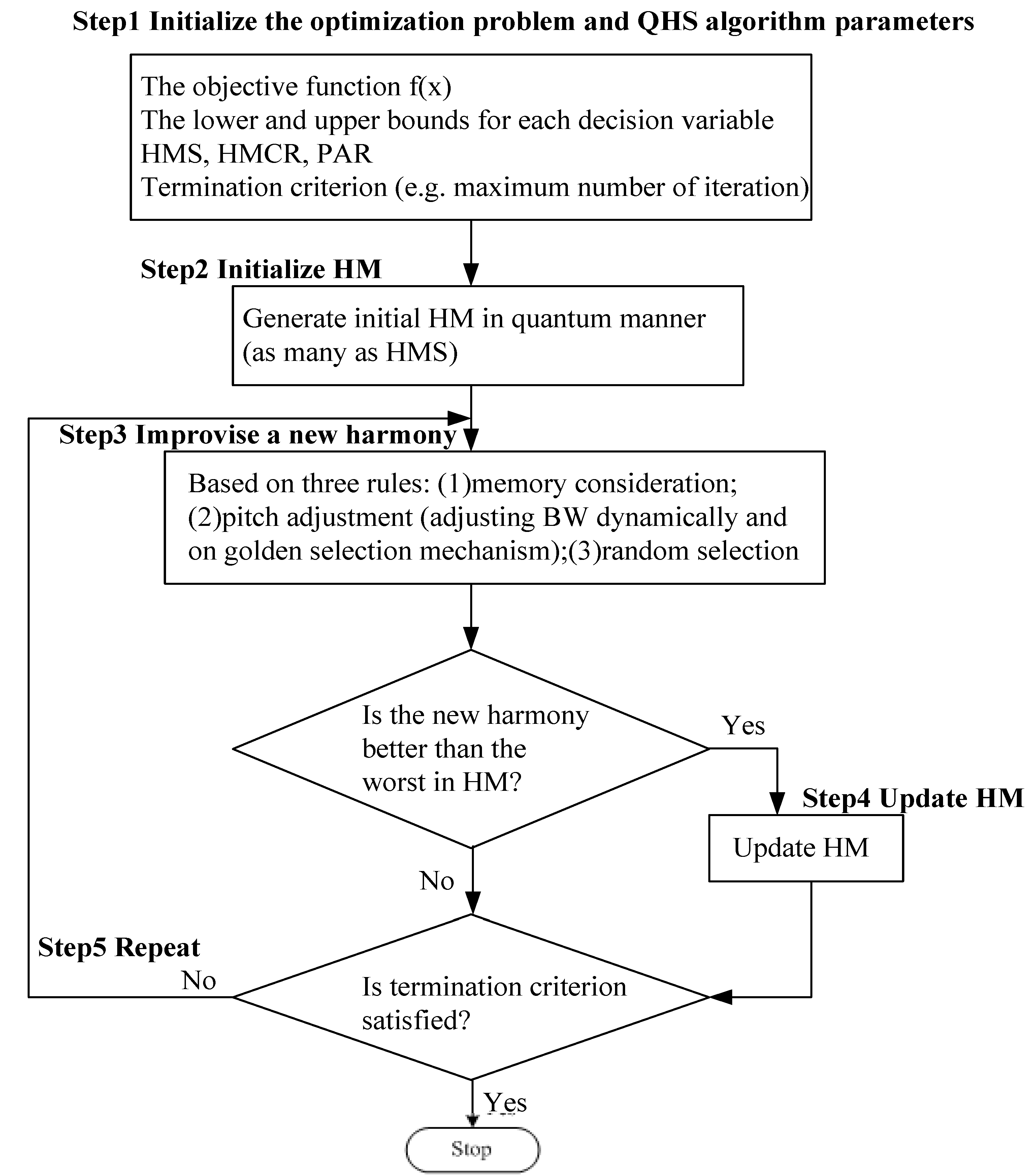
(2) The β optimization process based on the QHS algorithm
The optimization objective function f(x) of QHS algorithm is specified as the Mean Absolute Percentage Error (MAPE) in this proposed investigation. The MAPE is the measure of accuracy in a fitted time series value in statistics, specifically trending. It usually expresses accuracy as a percentage, eliminating the interaction between negative and positive values by taking absolute operation [10], shown in Equation (9):
M A P E = 1 T t = 1 T | y t y ^ t y t |
Minimize:
f ( x ) = 1 T t = 1 T | y t y ^ t y t | = 1 T t = 1 T { | y t i = 1 k [ t = 1 T β i t T t + 1 ( y t y ^ t ( i ) ) 2 ] 1 y ^ t ( i ) i = 1 k [ t = 1 T β i t T t + 1 ( y t y ^ t ( i ) ) 2 ] 1 | / | y t | } s . t . 0 β i t 1
The QHS optimization DMSFE approach has been employed to determine optimal βit values for the top-5 CO2 emitting countries. The QHS algorithm parameters are selected by uniform design [35] as follows: HMS = 35, HMCR = 0.99, PAR = 0.6, lb = 0, ub = 1, where lb is the lower bound for decision variable βit, ub is the upper bound for decision variable βit.
All the programs were run on a 2.27 GHz Intel Core Duo CPU with 1 GB of random access memory. In each case study, 30 independent runs were made for the QHS optimization procedure in MATLAB 7.6.0 (R2008a) on Windows 7 with 32-bit operating systems. Then, the best key was assigned as the optimal βit values for the corresponding individual model and period shown as follows:
β 1 = [ 3.0537 × 10 1 7.2000 × 10 1 9.4362 × 10 1 2.9229 × 10 1 8.3754 × 10 1 3.8874 × 10 1 9.9363 × 10 1 5.7866 × 10 1 5.0000 × 10 1 6.4622 × 10 1 9.9977 × 10 1 4.9153 × 10 1 7.5580 × 10 1 6.0927 × 10 1 7.9302 × 10 1 5.6514 × 10 1 8.5425 × 10 1 6.0933 × 10 1 9.9864 × 10 1 6.6901 × 10 1 1.6120 × 10 1 5.8412 × 10 1 9.9995 × 10 1 5.0000 × 10 1 2.4265 × 10 1 8.7951 × 10 1 9.9999 × 10 1 5.0000 × 10 1 9.9417 × 10 1 5.0000 × 10 1 9.4228 × 10 1 6.5848 × 10 1 7.7294 × 10 1 1.5657 × 10 3 1.0506 × 10 1 6.9660 × 10 1 1.2785 × 10 1 2.1846 × 10 1 9.5525 × 10 1 6.4635 × 10 1 6.4795 × 10 1 4.8761 × 10 1 9.5044 × 10 1 5.0000 × 10 1 ] T
β 2 = [ 9.9988 × 10 1 8.3856 × 10 1 9.8044 × 10 1 6.3427 × 10 1 1.0000 9.9652 × 10 1 5.8076 × 10 1 7.7253 × 10 1 9.8022 × 10 1 9.9697 × 10 1 9.0721 × 10 1 7.4681 × 10 1 9.1888 × 10 1 7.8330 × 10 1 8.3612 × 10 1 8.6807 × 10 1 9.9997 × 10 1 9.9932 × 10 1 3.0525 × 10 1 1.9819 × 10 1 9.9924 × 10 1 9.9957 × 10 1 8.5354 × 10 1 1.9655 × 10 1 9.9930 × 10 1 1.0000 3.5637 × 10 1 7.3147 × 10 1 9.8933 × 10 1 1.0000 2.1782 × 10 1 3.3123 × 10 1 9.9778 × 10 1 1.0000 9.8847 × 10 1 7.2151 × 10 1 1.0000 9.9967 × 10 1 2.5472 × 10 1 6.8253 × 10 1 5.3405 × 10 1 1.0000 9.9984 × 10 1 5.3690 × 10 1 ] T
β 3 = [ 9.9900 × 10 1 1.0000 9.9901 × 10 1 7.7889 × 10 1 1.2562 × 10 1 5.0620 × 10 1 7.3263 × 10 1 9.7903 × 10 1 3.3333 × 10 1 9.9053 × 10 1 9.9918 × 10 1 6.2317 × 10 1 9.9193 × 10 1 8.7692 × 10 1 9.3247 × 10 1 5.3028 × 10 1 9.9877 × 10 1 9.3810 × 10 1 9.8234 × 10 1 2.4884 × 10 1 1.0000 8.1265 × 10 1 9.3706 × 10 1 6.9827 × 10 1 2.6092 × 10 1 9.8815 × 10 1 4.9718 × 10 1 3.2615 × 10 1 9.9000 × 10 1 9.9444 × 10 1 9.9838 × 10 1 4.7104 × 10 1 8.0638 × 10 1 1.0000 9.9999 × 10 1 5.5961 × 10 2 9.9863 × 10 1 1.9856 × 10 1 1.0000 2.9490 × 10 2 4.5254 × 10 1 9.1639 × 10 1 9.9479 × 10 1 9.6163 × 10 1 ] T
β 4 = [ 1.0000 6.1020 × 10 1 8.2721 × 10 1 4.4806 × 10 1 4.3893 × 10 1 8.1632 × 10 1 7.8088 × 10 1 5.6974 × 10 1 8.1888 × 10 1 2.7395 × 10 1 7.4244 × 10 1 6.1378 × 10 1 9.9521 × 10 1 9.9430 × 10 1 9.1750 × 10 1 6.9563 × 10 1 1.0000 5.0596 × 10 2 1.0000 2.6973 × 10 1 9.8277 × 10 1 9.1807 × 10 1 7.6791 × 10 1 7.8573 × 10 1 1.0000 5.0589 × 10 1 9.5817 × 10 1 3.6899 × 10 1 9.9871 × 10 1 6.5940 × 10 1 5.9211 × 10 1 8.2182 × 10 1 9.3071 × 10 1 5.5626 × 10 1 1.4716 × 10 1 6.1601 × 10 1 9.8508 × 10 1 3.8165 × 10 1 4.5431 × 10 1 1.3320 × 10 1 9.9991 × 10 1 2.2622 × 10 1 8.7349 × 10 1 8.3105 × 10 1 ] T
β 5 = [ 9.9998 × 10 1 2.2472 × 10 1 9.7696 × 10 1 9.9998 × 10 1 1.0000 9.4249 × 10 1 6.8640 × 10 1 6.2069 × 10 1 9.2596 × 10 1 8.2604 × 10 1 2.4110 × 10 1 8.4266 × 10 1 8.0391 × 10 1 9.9758 × 10 1 8.5322 × 10 1 9.0891 × 10 1 6.6755 × 10 1 8.3244 × 10 1 3.9699 × 10 1 4.2721 × 10 1 8.8024 × 10 1 1.0666 × 10 1 3.1147 × 10 1 9.9761 × 10 1 9.3537 × 10 1 9.9998 × 10 1 5.0190 × 10 1 9.9998 × 10 1 7.2457 × 10 1 9.9982 × 10 1 2.6831 × 10 1 9.9999 × 10 1 1.0000 1.0000 2.8461 × 10 1 8.0354 × 10 1 9.9997 × 10 1 7.2360 × 10 1 1.5597 × 10 2 7.4259 × 10 1 9.4032 × 10 1 8.4071 × 10 1 4.9635 × 10 1 5.1870 × 10 1 ] T
where β 1 is the optimal β matrix for China, β 2 for US, β 3 for Russia, β 4 for India and β 5 for Japan. It could be found that the optimal βit values vary quite a lot from each other even for the same county. The data differ from each other heavily in the case of China. The situations of Russia and Japan are similar to it of China. In the first column of matrix, all data, with uniform magnitude, are very close or equal to 1.0000 except one in the case of USA. The situation of India is similar to that of the USA. From the final optimal β values, we can draw two conclusions: (1) the best β values may be different for different counties; (2) the best β values may be different for different individual models and forecasting periods, even in the same country, since β ranges from 0 to 1, therefore, the arbitrary selection of β may not result in the best combination forecast effect, i.e., not the minimal MAPE. Taking the same β for all individual models and forecasting period may bring the same drawback as the one above. It is vital to select suitable β values for the combination model. Through an optimization process, the best β values could be found with the minimal MAPE for combination forecast based on QHS algorithm. With these optimal β values the forecasting results and evaluating indexes could be obtained and presented in next sections.
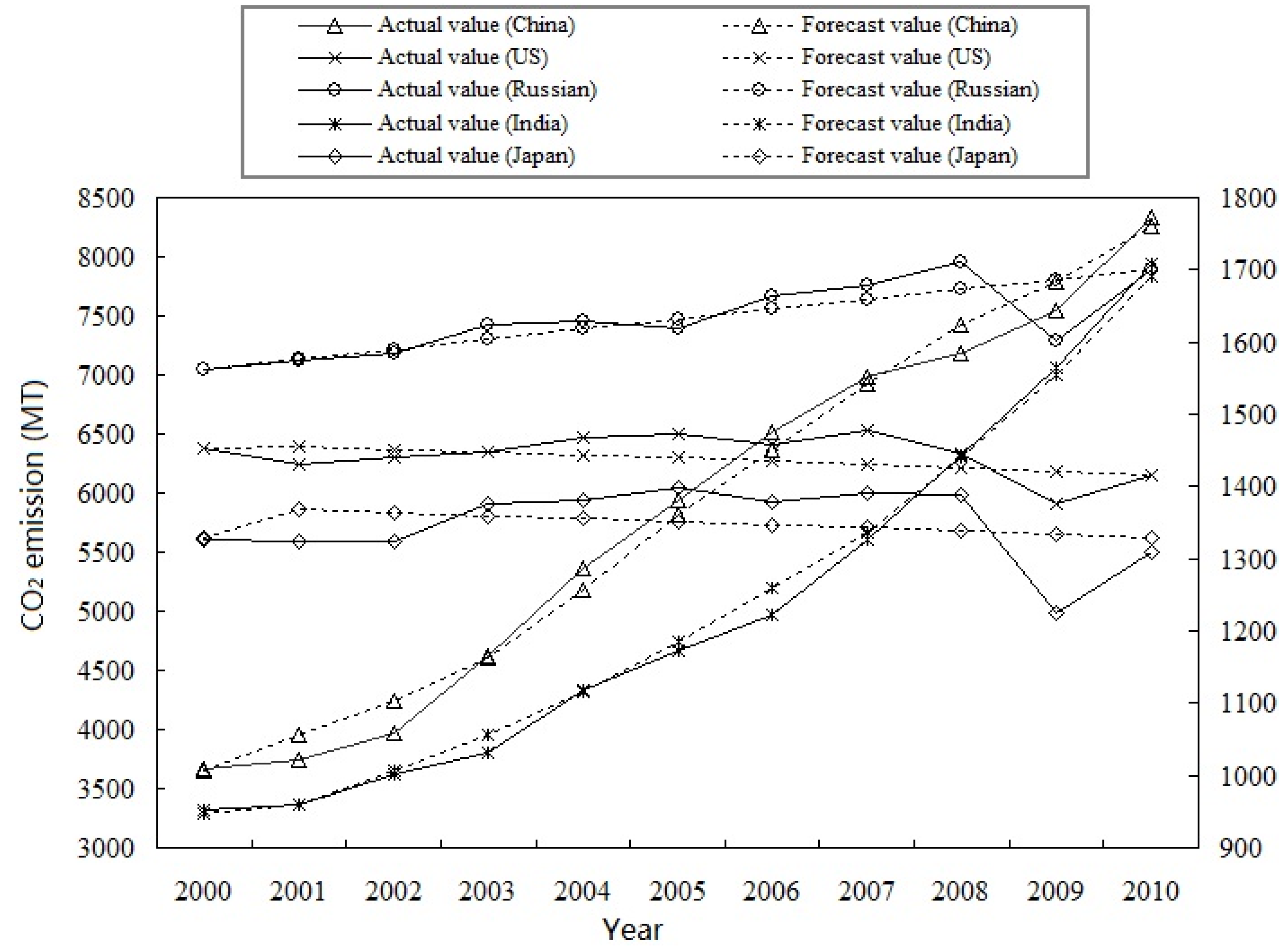
(3) The forecasting results
Figure 2 shows the curves of actual data and forecasting results achieved by the presented approach for the top-5 emitters from 2000 to 2010 respectively. Dual coordinates are employed in Figure 2: the curves of actual data and forecasting results for China and US correspond to the left y-axis coordinate; the curves of actual data and forecasting results for the other three countries correspond to the right y-axis coordinate. These five counties could be divided into two kinds according to the growth direction: (1) ascending cases such as China, India and Russia; (2) fluctuating cases such as the US and Japan. From Figure 2 we find that the forecasting results of China, Russia, India and US are relatively close to the original values at every point. For Japan, the proposed approach behaves well at some points and relatively poor at others. But, analyzing the MAPE in next section, the forecasting errors are acceptable, even in those poor situations. There is a sudden drop in the actual values of Russia, US and Japan between 2008 and 2010 because an abrupt economy crisis broke out around the World and resulted in lowered CO2 emissions in these countries. The forecasting results are relatively inaccurate in those years because of the abruptness. It is natural since there is no one method works well for all situations. Every method has its own application circumstance. The presented method forecasting results are satisfied for different growth pattern that means the flexibility of the QHS algorithm based DMFSE combination model is excellent.
Figure 2. Actual and forecast values for the World top-5 emitters.
Energies 06 01456 g002

3.3. Case Comparison

In order to testify the validity of the QHS algorithm-based DMFSE combination forecasting method, five cases were considered in this section: Case 1, β = 0.1; Case 2, β = 0.5; Case 3, β = 1; Case 4, β* (adopting the same optimal β value for all individual models and all forecasting periods obtained by QHS algorithm shown in Table 3; the parameters of QHS algorithm achieved by uniform design); Case 5, Dβ* (adopting the different optimal β values for different individual model and period obtained by QHS algorithm). We selected three cases near the beginning, middle and end of β span as examples since β varies from 0 to 1. Table 4, Table 5, Table 6, Table 7 and Table 8 show the combination forecasting results of different cases for China, US, Russian Federation, India and Japan respectively. From these tables we could find that the forecasting results obtained by the presented approach are the best in most situations for all the five counties.
Furthermore, the fitting effect is evaluated through some common evaluating indicators i.e., MAPE, RMSE and MAE shown in Equations (9), (11) and (12). The evaluating results are exhibited in Table 9, Table 10 and Table 11:
R M S E = 1 T t = 1 T ( y t y ^ t ) 2
M A E = 1 T t = 1 T | y t y ^ t |
Table 3. The optimal β values in case 4 for top-5 countries.
ChinaUnited StatesRussian FederationIndiaJapan
β*1.00002.2195 × 1052.9628 × 1052.7599 × 1051.0000
Table 4. Forecasting values with different cases for China (Mtonnes).
YeartOriginal dataβ = 0.1β = 0.5β = 1β*Dβ*
200013659.34833530.35723558.37333606.60733606.60733658.8771
200123736.97943932.19663942.47413959.64793959.64793959.8116
200233969.82314332.11114320.57214302.48154302.48154243.2317
200344613.92004761.49674734.98564693.82214693.82214599.3799
200455357.16515267.12575247.20985222.91765222.91765186.9109
200565931.97135795.67745787.73275788.97355788.97355825.7973
200676519.59656303.28876299.50066309.31826309.31826368.3617
200786979.46536823.70056827.15776848.88136848.88136930.0485
200897184.85427807.41747339.70237808.00817362.86267430.7278
2009107546.68298316.20677807.18458316.10727808.00817793.0080
2010118332.51588348.39398320.28938348. 59528316.10728251.4506
Table 5. Forecasting values with different cases for the United States (Mtonnes).
YeartOriginal dataβ = 0.1β = 0.5β = 1β*Dβ*
200016377.04936381.02506373.78126380.14816386.21806377.5702
200126248.36086375.78276368.48826378.66976385.28356388.6531
200236296.22486353.70946345.66266356.38696363.67826366.5027
200346343.47696330.78896322.15676333.61676341.37996343.6542
200456472.44636306.95316297.91416310.31766318.33246320.0496
200566493.73416282.12966272.87506286.44606294.47626295.6276
200676411.95036256.24286246.97706261.95616269.74886270.3240
200786523.79876229.21306220.15436236.79986244.08486244.0715
200896332.60046200.95746192.33856210.92686217.41586216.7998
2009105904.03826171.38986163.45856184.28536189.67096188.4359
2010116144.85106140.42176133.44116156.82156160.77716158.9047
Table 6. Forecasting values with different cases for the Russian Federation (Mtonnes).
YeartOriginal dataβ = 0.1β = 0.5β = 1β*Dβ*
200011562.97911567.46181570.73261570.57841563.00581563.1559
200121574.49291583. 86751586.38491586.19431576.68641576.8574
200231583.98951595.84941597.79641597.65001590.35561590.4870
200341624.76821607.78651609.00651608.90941604.04051604.1273
200451628.03501619.69251620.05891620.01541617.73951617.7777
200561618.00461631.57881630.98911631.00241631.45071631.4374
200671663.33231643.45451641.82531641.89801645.17251645.1050
200781678.72761655.32661652.59041652.72451658.90301658.7795
200891711.08661667.20101663.30291663.49981672.64071672.4596
2009101602.52121679.08201673.97741674.23831686.38351686.1438
2010111700.19921690.97341684.62571684. 95151700.13001699.8306
Table 7. Forecasting values with different cases for India (Mtonnes).
YeartOriginal dataβ = 0.1β = 0.5β = 1β*Dβ*
20001952.7665942.7369942.0609940.7183942.7948946.7714
20012959.1636946.7968944.4024945.9440947.4891959.1655
200231001.2000999.7583998.5021998.95271000.12311005.5160
200341030.47141056.82411056.71041055.84111056.84881055.8330
200451118.36461120.39211121.05921119.44261120.18851114.9742
200561172.86311191.53191192.53141190.85671191.23801184.5290
200671222.40881269.02371270.29571268.21121268.63891260.5112
200781327.07711351.21711353.31761348.98231350.55621337.5920
200891442.15291449.86651451.03151447.44991449.43361441.1711
2009101563.91721558.70551559.04651554.84121558.44751553.8716
2010111707.45941685.99681684.44261680.36831686.21541690.9122
Table 8. Forecasting values with different cases for Japan (Mtonnes).
YeartOriginal dataβ = 0.1β = 0.5β = 1β*Dβ*
200011327.13241335.78701337.94971340.21271340.21271328.2275
200121324.44861345.35181348.55901352.54961352.54961368.1131
200231322.95231342.57411346.18921350.66581350.66581363.8899
200341376.25071339.58901343.55681348.44941348.44941359.6458
200451380.79131336.46051340.76321346.04931346.04931355.3961
200561397.70161333.21951337.85931343.54091343.54091351.1491
200671379.29971329.87981334. 86951340.96171340.96171346.9085
200781392.12971326.44681331.80501338.33051338.33051342.6762
200891389.35731322.92141328.67031335.65601335.65601338.4531
2009101225.48101319.30211325.46611332.94181332.94181334.2398
2010111308.39581315.58611322.19151330.18901330.18911330.0362
Table 9. MAPE values with different case for top-5 countries (%).
Countryβ = 0.1β = 0.5β = 1β*Dβ*
China3.30113.22853.06013.06012.6211
United States2.05942.11042.04942.02822.0135
Russian Federation1.31831.40031.39591.18541.1894
India1.32491.41441.35371.30100.9462
Japan3.22633.18943.14153.14152.9949
Table 10. MAE values with different case for top-5 countries (Mtonnes).
Countryβ = 0.1β = 0.5β = 1β*Dβ*
China1.6886 × 1021.6659 × 1021.6017 × 1021.6017 × 1021.4196 × 102
United States1.3022 × 1021.3357 × 1021.2943 × 1021.2797 × 1021.2703 × 102
Russian Federation2.1597 × 102.2967 × 102.2893 × 101.9402 × 101.9469 × 10
India1.6003 × 101.7051 × 101.6466 × 101.5728 × 101.1539 × 10
Japan4.3382 × 104.2723 × 104.1881 × 104.1881 × 103.9763 × 10
Table 9 shows the MAPE values of different β values for these five countries. The MAE values for all situations for all the five countries are shown in Table 10. The MAPE and MAE values of Dβ* are the least in five situations for China, USA, India and Japan. The MAPE and MAE values of Dβ* are better than those of βs obtained arbitrarily, but worse a little than β* for Russia. Actually, they are very close to those of β* for Russia. Comparing the MAPE and MAE results of β* and Dβ* with those of the other three βs shown in Table 9 and Table 10 it could be found: (1) the MAPE and MAE values of the first three βs are close to each other; (2) the MAPE and MAE values of β* increase to a certain extent for USA and India; (3) the MAPE and MAE values of β* are the same as those of β = 1 and better than those of β = 0.1 and β = 0.5 for China and Japan; (4) the MAPE and MAE values of β* are the best among the five cases for Russia; (5) the MAPE and MAE values of Dβ* are improved relatively remarkably for all five countries, especially in the case of India compared with those of βs obtained arbitrarily; (6) the MAPE and MAE values of Dβ* are the best among all five cases for all countries except Russia; (7) the MAPE and MAE values of Dβ* are better than those of βs obtained arbitrarily and close to those of β* for Russia. The results of β* for China and Japan are the same as those of β = 1 because the optimal β values found are 1. The results of β* show that adopting an optimization method to choose an optimal β value is better than the method of assigning β values arbitrarily. The results of Dβ* indicate that considering different individual models and periods is better than applying one β value to all separate models and periods. The empirical results suggest that QHS algorithm-based combination forecasting method enhances the MAPE and MAE to a certain degree for every country, especially for India. Namely, the proposed method outperforms all the other methods concerned. For India, the MAPE increases from over 1.3249% to 0.9462% and the MAE increases from over 16.003 Mtonnes to 11.539 Mtonnes. It means over 28% performance enhancement compared with the original method. It enhances over 14% in the case of China. For Russian it improves by over 10%. It increases relatively indistinctively only in the case of Japan and US, near 5% and 2%, respectively.
The RMSE values of all situations for five countries are shown in Table 11. The results of Dβ* are the best among all five situations for all countries, except Russia. The RMSE results for Russia presents an opposite situation compared with the status when considering the MAPE values viz. the results of β* and Dβ* are worse than those of β = 0.1, β = 0.5 and β = 1. The RMSE value of Dβ* is better than that of β* for Russia. The RMSE value for India of Dβ* is improved over 22.3% compared with the original method. It increases over 6.7% for China, 1.5% for USA and 1.7% for Japan. The RMSE values of β* for USA and India are enhanced too compared with those of β = 0.1, β = 0.5 and β = 1. China and Japan share the same RMSE value of β = 1 and β* for the reason mentioned last paragraph. And the values of β* are better than those of β = 0.1, β = 0.5. All these again show that adopting the optimization method to choose an optimal β value is better than the method of assigning β value arbitrarily. The method taking different individual models and periods into consideration is the best among all the methods. The conclusion is the same as the one drawn when discussing the MAPE index.
Table 11. RMSE values with different case for top-5 countries (Mtonnes).
Countryβ = 0.1β = 0.5β = 1β*Dβ*
China1.8966 × 1021.8748 × 1021.8325 × 1021.8325 × 1021.7000 × 102
United States1.6285 × 1021.6600 × 1021.6190 × 1021.5966 × 1021.5951 × 102
Russian Federation2.9552 × 102.9619 × 102.9606 × 103.0144 × 103.0113 × 10
India2.0462 × 102.1386 × 102.0705 × 102.0218 × 101.5907 × 10
Japan5.0801 × 104.9519 × 104.8536 × 104.8536 × 104.7725 × 10
According to the discussions above, the presented method shows the best MAPE, RMSE and MAE performance among the five situations for all countries, except Russia. For Russia the proposed method shows a better RMSE performance than the method of applying the same optimal β value for all individual models and forecasting periods. A better MAPE and MAE performance are obtained by the presented method compared with those of the original method. All in all the presented approach could provide a relatively better forecasting performance in comparison with the methods of choosing β values arbitrarily and assigning the same optimal β value to all individual models synthesizing the MAPE, RMSE and MAE indexes discussed above. The analysis based on MAPE, RMSE and MAE indicates that the proposed method has a good robustness to the choice of index for forecasting accuracy.

3.4. Analysis of Future Projections

In order to evaluate the out-of-sample forecasting performance of the proposed approach, the forecasting values calculated with the optimal β values obtained in Section 3.2 and the relative errors between the forecasting values and the actual values of the year 2011 are shown in Table 12. The forecasting performance is relatively nice for all the five countries, especially for China.
The forecasting values of the year 2012–2015 are shown in Table 13. We could find that the trend of the CO2 emissions for China and India is increasing and it is fluctuating for USA, Russia and Japan based on the analysis of the forecasting values. These trends are consistent with the expectations. The situation is very critical since CO2 has so many detrimental impacts on our living environment. The technical improvements and energy policies of the government should be made to reduce the emissions.
Table 12. Forecasting values and relative errors of 2011 for top-5 countries.
ChinaUSARussiaIndiaJapan
Original data (Mtonnes)8979.14116016.61271675.03551797.98791307.4005
Forecasting data (Mtonnes)8947.83746134.12581712.95651855.51831324.2965
Relative error (%)0.34861.95312.26393.19971.2923
Table 13. Forecasting values of 2012–2015 for top-5 countries (Mtonnes).
Country2012201320142015
China9268.56009821.047610391.812310981.5386
USA6102.28106068.91206034.09065997.7174
Russia1727.07711740.76051754.44311768.1233
India2039.15022291.27372641.23303182.6860
Japan1321.49041317.36571313.25131309.1472

4. Conclusions

As Hibon pointed out, no one forecasting model can outperform others in all circumstances [18]. Choosing a combination method could lead to less risk than choosing one single method. The DMSFE combination method was applied in this work to forecast CO2 emissions. The individual forecasting method was first selected to establish the combination model. Then, the QHS algorithm was introduced to search for the optimal discounting factor β values for each individual model and forecasting period. Finally, the combination forecasting results were obtained. In the DMSFE combination forecasting method, how to select the β value is a key problem since it varies between 0 and 1 and influences the forecasting results directly. However, it is hard to choose the appropriate β values for decision-makers only by arbitrary attempts, and this manner often leads an unsatisfactory forecasting performance. Assigning the same β value for all separate models and forecasting period in all application cases is somewhat unreasonable since it affects the proportion of each individual model forecasting results in the combination model forecasting results. Applying different β values to different individual models and forecasting periods sounds more suitable. Thus, β was changed from one value to a matrix to express the influences of the individual models and forecasting periods. It is difficult to seek the optimal matrix by traditional mathematical methods since there are so many parameters to be optimized. The optimization algorithm provides a valid way to solve these problems through optimizing objective function (MAPE in this work) to find the optimal β values. A novel and effective intelligence optimization method called QHS algorithm was applied in this investigation to find the optimal β values for every individual forecasting model and forecasting period in the combination model. The empirical analysis applied to the World’s top-5 emitters shows that the QHS- based optimization DMSFE combination method performs much better than the original method with an arbitrarily chosen parameter β value. The contributions of this work are as follows: (1) The optimal discounting factor β can be determined by using an optimization technique; (2) Applying different β values to different individual models and forecasting periods is more reasonable than the manner where the same value is applied to all separate models; (3) The QHS-based combination forecasting model can increase forecasting accuracy in a certain degree.

Acknowledgments

This work was supported by “the Fundamental Research Funds for the Central Universities (12MS137)”.

References

  1. International Energy Agency (IEA). World Energy Outlook 2010; International Energy Agency (IEA): Paris, France, 2010; Available online: http://www.iea.org/publications/freepublications/publication/name,27324,en.html (accessed on 9 April 2012).
  2. Suganthi, L.; Samuel, A.A. Energy models for demand forecasting—A review. Renew. Sustain. Energy Rev. 2012, 16, 1223–1240. [Google Scholar] [CrossRef]
  3. Wang, W.; Kuang, Y.; Huang, N. Study on the decomposition of factors affecting energy-related carbon emissions in Guangdong province, China. Energies 2011, 4, 2249–2272. [Google Scholar] [CrossRef]
  4. Akbostancı, E.; Tunç, G.I.; Aşık, S.T. CO2 emissions of Turkish manufacturing industry: A decomposition analysis. Appl. Energy 2011, 88, 2273–2278. [Google Scholar] [CrossRef]
  5. Meng, M.; Niu, D. Modeling CO2 emissions from fossil fuel combustion using the logistic equation. Energy 2011, 36, 3355–3359. [Google Scholar] [CrossRef]
  6. Tutmez, B. Trend analysis for the projection of energy-related carbon dioxide emissions. Energy Explor. Exploit. 2006, 24, 139–150. [Google Scholar] [CrossRef]
  7. Köne, A.Ç.; Büke, T. Forecasting of CO2 emissions from fuel combustion using trend analysis. Renew. Sustain. Energy Rev. 2010, 14, 2906–2915. [Google Scholar] [CrossRef]
  8. Raghuvanshi, S.P.; Chandra, A.; Raghav, A.K. Carbon dioxide emissions from coal based power generation in India. Energy Convers. Manag. 2006, 47, 427–441. [Google Scholar] [CrossRef]
  9. Liang, Q.M.; Fan, Y.; Wei, Y.M. Multi-regional input–output model for regional energy requirements and CO2 emissions in China. Energy Policy 2007, 35, 1685–1700. [Google Scholar] [CrossRef]
  10. Chen, T.; Wang, Y. A fuzzy-neural approach for global CO2 concentration forecasting. Intell. Data Anal. 2011, 15, 763–777. [Google Scholar]
  11. Sun, J.W. An alternative viewpoint on the forecasting of energy-related CO2 emissions in the OECD countries. Energy Policy 2006, 34, 377–382. [Google Scholar] [CrossRef]
  12. Pao, H.T.; Tsai, C.H. Modeling and forecasting the CO2 emissions, energy consumption, and economic growth in Brazil. Energy 2011, 36, 2450–2458. [Google Scholar] [CrossRef]
  13. Lin, C.S.; Liou, F.M.; Huang, C.P. Grey forecasting model for CO2 emissions: A Taiwan study. Appl. Energy 2011, 88, 3816–3820. [Google Scholar] [CrossRef]
  14. Ramanathan, R. An analysis of energy consumption and carbon dioxide emissions in countries of the Middle East and North Africa. Energy 2005, 30, 2831–2842. [Google Scholar]
  15. Rout, U.K.; Voβ, A.; Singh, A.; Fahl, U.; Blesl, M.; Gallachóir, B.P. Energy and emissions forecast of China over a long-time horizon. Energy 2011, 36, 1–11. [Google Scholar] [CrossRef]
  16. He, J.K.; Deng, J.L.; Su, M.S. CO2 emission from China’s energy sector and strategy for its control. Energy 2010, 35, 4494–4498. [Google Scholar] [CrossRef]
  17. Bates, J.M.; Granger, C.W. The combination of forecasts. Opl. Res. Q. 1969, 20, 451–468. [Google Scholar] [CrossRef]
  18. Hibon, M.; Evgeniou, T. To combine or not to combine: Selecting among forecasts and their combinations. Int. J. Forecast. 2005, 21, 15–24. [Google Scholar] [CrossRef]
  19. Zhang, G.P. Time series forecasting using a hybrid ARIMA and neural network model. Neurocomputing 2003, 50, 159–175. [Google Scholar] [CrossRef]
  20. Winkler, R.L.; Makridakis, S. The combination of forecasts. J. R. Stat. Soc. A 1983, 146, 150–157. [Google Scholar] [CrossRef]
  21. Geem, Z.W.; Kim, J.H.; Loganathan, G.V. A new heuristic optimization algorithm: Harmony search. Simulation 2001, 76, 60–68. [Google Scholar] [CrossRef]
  22. Lee, K.S.; Geem, Z.W. A new meta-heuristic algorithm for continues engineering optimization: Harmony search theory and practice. Comput. Method Appl. Mech. Eng. 2005, 194, 3902–3933. [Google Scholar] [CrossRef]
  23. Mahdavi, M.; Fesanghary, M.; Damangir, E. An improved harmony search algorithm for solving optimization problems. Appl. Math. Comput. 2007, 188, 1567–1579. [Google Scholar] [CrossRef]
  24. Geem, Z.W.; Kim, J.H.; Loganathan, G.V. Harmony search optimization: Application to pipe network design. Int. J. Model. Sim. 2002, 22, 125–133. [Google Scholar]
  25. Yadav, P.; Kumar, R.; Panda, S.K.; Chang, C.S. An intelligent tuned harmony search algorithm for optimization. Inf. Sci. 2012, 196, 47–72. [Google Scholar] [CrossRef]
  26. Al-Betar, M.A.; Doush, I.A.; Khader, A.T.; Awadallah, M.A. Novel selection schemes for harmony search. Appl. Math. Comput. 2012, 218, 6095–6117. [Google Scholar] [CrossRef]
  27. Han, K.H.; Kim, J.H. Quantum-inspired algorithm for a class of combinational optimization. IEEE Trans. Evolut. Comput. 2002, 6, 580–593. [Google Scholar] [CrossRef]
  28. Wang, C.M.; Huang, Y.F. Self-adaptive harmony search algorithm for optimization. Expert Syst. Appl. 2010, 37, 2826–2837. [Google Scholar] [CrossRef]
  29. Chang, H.; Gu, X.S. Multi-HM adaptive harmony search algorithm and its application to continuous function optimization. Res. J. Appl. Sci. Eng. Tech. 2012, 4, 100–103. [Google Scholar]
  30. British Petroleum (BP). BP Energy Outlook 2030; BP: London, UK, 2011; Available online: http://www.bp.com/energyoutlook2030 (accessed on 9 April 2012).
  31. Hubacek, K.; Feng, K.; Chen, B. Changing lifestyles towards a low carbon economy: An IPAT analysis for China. Energies 2012, 5, 22–31. [Google Scholar] [CrossRef]
  32. Chatfield, C. The Analysis of Time Series, An Introduction, 6th ed.; Chapman & Hall/CRC: New York, NY, USA, 2004. [Google Scholar]
  33. Deng, J.L. Grey System Fundamental Method; Huazhong University of Science and Technology Press: Wuhan, China, 1982. [Google Scholar]
  34. Wen, K.L.; Chang, T.C. The Research and Development of Completed GM (1, 1) Model Toolbox Using Matlab. Int. J. Comput. Cognit. 2005, 3, 42–48. [Google Scholar]
  35. Fang, K.T. Uniform Design and Uniform Design Table; Science Publishing House: Beijing, China, 1994. [Google Scholar]

Appendix

Table A1. Actual and forecasted value of China’s CO2 emissions (Mtonnes).
YeartOriginal dataLinearTime seriesGM(1,1)Grey Verhulst
200013659.34833341.88083805.33263659.34833659.3483
200123736.97943834.09233986.79854030.34374041.8571
200233969.82314326.30384127.37884380.28364450.4295
200344613.92004818.51534392.49034760.60754884.0364
200455357.16515310.72685075.63125173.95355341.0744
200565931.97135802.93845844.99865623.18895819.3488
200676519.59656295.14996428.73316111.42976316.0849
200786979.46536787.36147041.10866642.06266827.9699
200897184.85427279.57297535.35377218.76857351.2249
2009107546.68297771.78447769.87267845.54767881.7080
2010118332.51588263.99598179.27988526.74778415.0396
2011128979.14118756.20759015.30209267.09388946.7454
2012139248.41909133.150610071.72149472.4053
2013149740.63059704.686810946.21209987.7987
20141510232.842010311.988911896.631310489.0362
20151610725.053510957.294712929.572010972.6686
Table A2. Actual and forecasted value of the United States’ CO2 emissions (Mtonnes).
YeartOriginal dataLinearTime seriesGM(1,1)Grey Verhulst
200016377.04936419.36686185.19706377.04936377.0493
200126248.36086400.01226143.74456415.67476356.7048
200236296.22486380.65756102.56986393.57926334.5820
200346343.47696361.30296061.67116371.55986310.5402
200456472.44636341.94836021.04656349.61636284.4300
200566493.73416322.59375980.69426327.74836256.0938
200676411.95036303.23915940.61236305.95566225.3658
200786523.79876283.88455900.79906284.23806192.0722
200896332.60046264.52995861.25256262.59526156.0317
2009105904.03826245.17535821.97116241.02696117.0562
2010116144.85106225.82065782.95296219.53296074.9517
2011126016.61276206.46606053.46906198.11306029.5197
2012136187.11146180.48056176.76685980.5582
2013146167.75686146.28236155.49415927.8637
2014156148.40226112.27346134.29475871.2337
2015166129.04766078.45276113.16835810.4687
Table A3. Actual and forecasted value of the Russian Federation’s CO2 emissions (Mtonnes).
YeartOriginal dataLinearTime seriesGM(1,1)Grey Verhulst
200011562.97911571.52511595.71451562.97911562.9791
200121574.49291583.54981604.72341587.72061576.6415
200231583.98951595.57451611.98791598.79911590.3213
200341624.76821607.59931617.84581609.95481604.0169
200451628.03501619.62401622.56941621.18841617.7264
200561618.00461631.64871626.37851632.50031631.4482
200671663.33231643.67351629.45001643.89121645.1804
200781678.72761655.69821631.92671655.36161658.9213
200891711.08661667.72301633.92401666.91201672.6692
2009101602.52121679.74771635.53441678.54301686.4222
2010111700.19921691.77241636.83311690.25511700.1786
2011121675.03551703.79721664.25501702.04901713.9367
2012131715.82191717.95851713.92521727.6946
2013141727.84661731.54701725.88421741.4505
2014151739.87141745.24311737.92671755.2028
2015161751.89611759.04741750.05321768.9495
Table A4. Actual and forecasted value of India’s CO2 emissions (Mtonnes).
YeartOriginal dataLinearTime seriesGM(1,1)Grey Verhulst
20001952.7665853.7771941.3825952.7665952.7665
20012959.1636928.4370974.8739911.6569989.5973
200231001.20001003.0970998.0749974.39711031.2846
200341030.47141077.75691020.97151041.45501078.8060
200451118.36461152.41681066.00521113.12791133.4199
200561172.86311227.07681137.16551189.73331196.7737
200671222.40881301.73671207.25581271.61071271.0674
200781327.07711376.39671239.90651359.12291359.3059
200891442.15291451.05661360.18181452.65761465.7047
2009101563.91721525.71651459.73311552.62951596.3681
2010111707.45941600.37651597.11581659.48131760.4798
2011121797.98791675.03641748.02601773.68681972.5260
2012131749.69641814.75201895.75182256.7673
2013141824.35631951.51732026.21732657.1569
2014151899.01622098.58962165.66153262.4076
2015161973.67622256.74562314.70224282.4294
Table A5. Actual and forecasted value of Japan’s CO2 emissions (Mtonnes).
YeartOriginal dataLinearTime seriesGM(1,1)Grey Verhulst
200011327.13241359.45241342.84581327.13241327.1324
200121324.44861357.08811347.38441369.63581323.8707
200231322.95231354.72381349.70481365.16301320.4393
200341376.25071352.35951350.89111360.70481316.8304
200451380.79131349.99521351.49761356.26111313.0358
200561397.70161347.63091351.80771351.83201309.0473
200671379.29971345.26671351.96621347.41731304.8563
200781392.12971342.90241352.04731343.01701300.4539
200891389.35731340.53811352.08871338.63111295.8312
2009101225.48101338.17381352.10991334.25951290.9789
2010111308.39581335.80951352.12071329.90221285.8877
2011121307.40051333.44521294.88011325.55921280.5479
2012131331.08091337.96471321.23031274.9498
2013141328.71661338.87131316.91551269.0835
2014151326.35231339.77861312.61491262.9392
2015161323.98801340.68651308.32831256.5068

