Natural Gas Prices on Three Continents

Abstract

We investigate the pricing formation of natural gas markets on three different continents (Europe, Asia and North America). We find that natural gas markets showed a strong relationship with the crude oil market between 1992 and 2001 and natural gas prices tended to thermal parity with crude oil prices. From 2002 natural gas markets exhibited a less pronounced relationship with the crude oil market and major natural gas markets were severely underpriced compared to crude oil. A globally integrated natural gas market, comparable to the global oil market, has not evolved. The main natural gas markets, however, exhibit some level of integration, especially over a longer time. The European market exhibits the strongest levels of integration, while the North American market exhibits the weakest.

1. Introduction

This paper investigates the price formation and the relationship of major natural gas benchmarks to the market for oil. Theoretically, natural gas prices should exhibit a long-term relationship with oil prices since natural gas and oil can substitute for each other. Oil can always be substituted for natural gas, but the reverse substitution is more complex because of the low energy density of natural gas. For example, oil is easier to ship and can be used more efficiently as automotive fuel. However, an increase in liquefaction and regasification capacity has contributed to the more efficient transportation of natural gas, hence world Liquefied Natural Gas (LNG) trading more than doubled from 137 billion cubic meters in 2000 to 298 billion cubic meters in 2010 [1].

Because of the theoretical link between oil and natural gas and because oil is traded frequently and globally and therefore has an established price, a large number of exporters price natural gas based on oil. According to the [2], for example, Russia imposes a natural gas indexation that pegs over 80% of natural gas price to fuel oil products. This number varies regionally: for Western Europe it is around 80% and for Eastern Europe it is over 95%. Similarly, LNG is pegged to crude oil or oil products [3]. Conversely, US gas is priced entirely on its own and any link between them is due to the fact they are substitutes. Oil and natural gas can be considered close substitutes in the long run since even cars can shift from gasoline to natural gas if it is economical. One can thus expect that oil and natural gas prices have a long-term equilibrium level to which they revert after longer or shorter swings. The empirical results of this paper show that they have indeed tended to revert to the so-called thermal parity; that is, to the level when the same calorific value of oil or crude oil is priced at the same level. However since 2006 US gas prices have gradually shown less sensitivity to the crude oil price. The weaker link between US natural gas prices and crude oil prices can be explained by the changed US position in the natural gas market. The US was a net natural gas importer; however, recent technological advances, such as horizontal drilling and hydraulic fracturing have resulted in an oversupply of natural gas.

Gas prices of the other two main consuming regions; Europe and Asia have recently also showed relaxation from oil-linkage. Before 2002, Japanese LNG was only slightly underpriced; however, after the market entrance of China, long-term natural gas contracts were renegotiated and the sensitivity of LNG prices to oil prices was reduced. Therefore, Japanese LNG became more severely underpriced as crude oil prices were rising between 2002 and 2010. Russian gas prices have still been linked to crude oil, but for example the Russian gas monopoly, Gazprom had to give concessions to European importers during 2008–2009 to tackle competition from spot LNG trading.

As US gas prices do not revert back to thermal parity but Asian and European gas prices are still priced on crude oil prices, the relationship between the US and the European/Asian gas markets has been challenged. The question is whether the separation of the US natural gas market is a temporary or long-term phenomenon. In the long run, a global natural gas market might evolve. Such a market would be integrated, and in equilibrium the global price would reflect thermal parity, hence, under an unsegmented global gas market, any permanent divergence from the oil market would not be likely. This view is strengthened by [4] as they find that there is a stable relationship between the oil and natural gas markets even if there are periods when crude oil and natural gas prices may seem to have separated. Similarly, [5,6,7] argue that natural gas prices are strongly related to crude oil prices.

2. Data

Average monthly commodity prices are obtained from the IMF Primary Commodity Prices database for the period of January 1992–December 2010. Oil price is considered to be an average of three benchmark oil prices: the US West Texas Intermediate (WTI), the UK Brent and the Dubai Fateh [8]. The oil market is thought to be global and unsegmented [9].

We analyze the three most important natural gas benchmark prices: the HH price, the Russian natural gas price and the Japanese LNG price. HH natural gas is the benchmark for the North-American market, as it is the most frequently traded and the most frequently traded natural gas contract.

The Russian clearing price, CIF Germany (the price includes the freight to the German border), which is determined based on long-term contracts is employed as a benchmark for Europe. Russia accounts for the largest portion of the EU’s natural gas imports in the period investigated. In 2001, 58% (51%) of the EU’s imports (including LNG) came from Russia. By 2005, Russia’s importance dropped to 50% (43%), and by 2010, it dropped to 44% (33%) due to increasing imports from Norway and the surge in LNG imports from the Middle East [10]. Over the investigated period, Russia was the largest exporter to the EU, and Russian exports accounted for approximately one quarter of EU consumption [1]. By 2020 Europe could rely on Russia for more than 40% of its natural gas demand because natural gas consumption is expected to rise in an effort to reduce carbon dioxide emissions [11].

As a robustness check we also present the results for the UK NBP (National Balancing Point) price, which is the most liquid traded contract for Europe; however, it is only available since October 1998. NBP is the leading traded benchmark for natural gas in Europe; even spot LNG trading is often linked to the NBP price. In addition, in a recent study, [12] show that the continental European gas markets exhibit a high order of integration with the NBP. Thus, the NBP can be an appropriate proxy for European natural gas in addition to the Russian benchmark.

The Japanese LNG price is a benchmark for Asia. In 2010, the Asia-Pacific region had an approximately 60% share of global LNG imports. Japan alone accounts for 31% of global imports, and South Korea accounts for another 15% [1]. LNG pricing in the Asia-Pacific region is based mainly on long-term contracts, and the pricing is linked to spot crude oil prices. Recently LNG shipments have more often been priced on the spot market; spot trading represents approximately 20% of all LNG produced annually [13].

In the IMF database US and Russian natural gas prices are quoted in dollars per thousand cubic meters, while LNG is quoted in dollars per cubic meter. We exchange these values to $/MMBtu (million British thermal units) using energy equivalents. Unless noted otherwise, hereinafter oil price is quoted in US dollars per barrel ($/bbl). A thousand cubic meters of US natural gas has a calorific value of 36.268 MMBtu [14]. Russian natural gas has a somewhat inferior energy density of 36.093 MMBtu per thousand cubic meters. The energy equivalent of one barrel of crude oil is 5.8 MMBtu, thus the energy density of crude oil is 36.481 MMBtu per cubic meter. LNG has an energy density of 23.8 MMBtu per cubic meter.

Descriptive Statistics

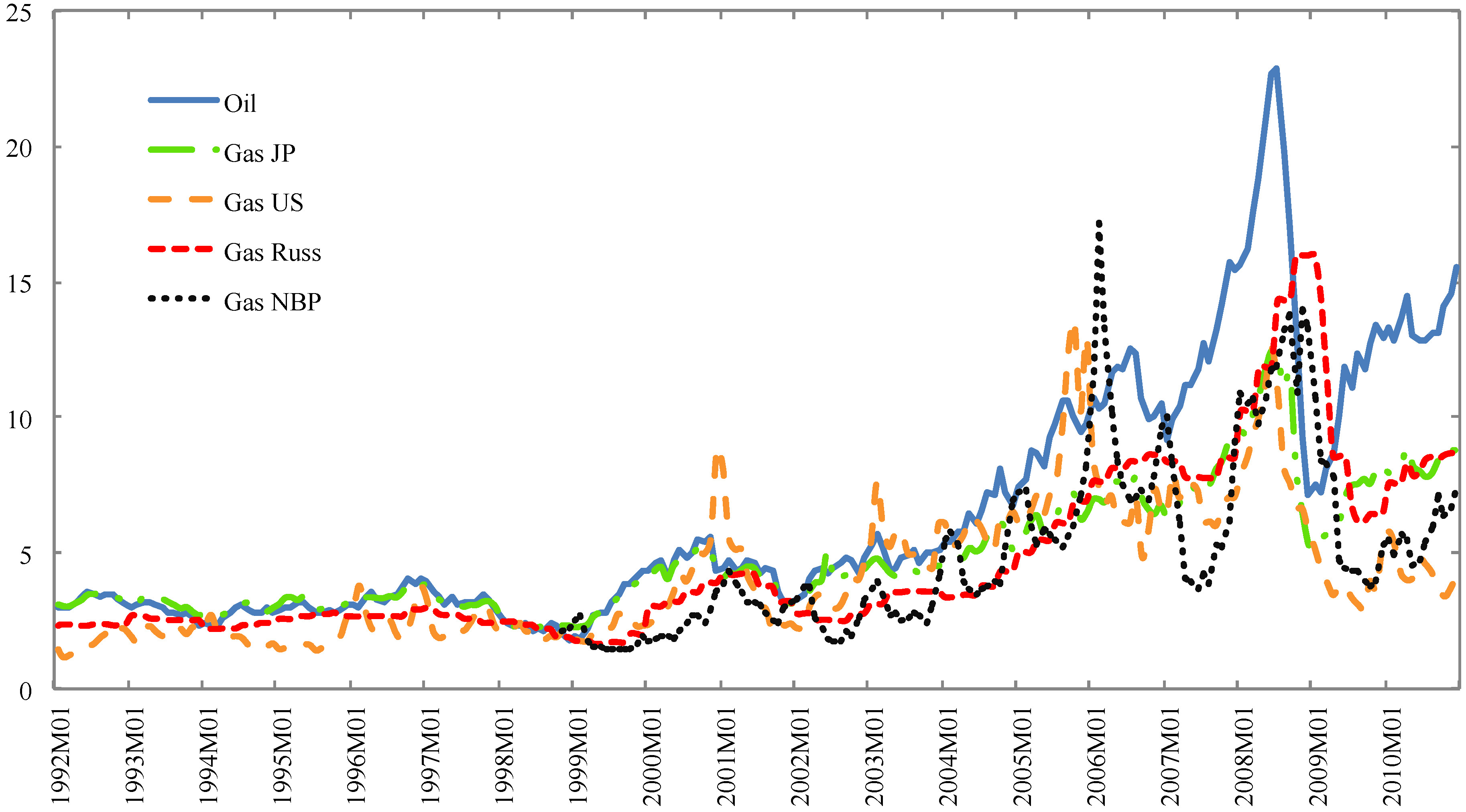
Figure 1 shows the US, Russian and NBP natural gas prices, the Japanese LNG price and the price of crude oil in $/MMBtu between 1992 and 2010. Until 2002, natural gas prices followed crude oil prices and were determined close to thermal parity. In the pre-2002 period only the US gas price separated from crude oil and only permanently during the so-called California energy crisis See the lessons of the California energy crisis in [15]. After 2002, crude oil and natural gas prices exhibited a weaker relationship.

Figure 1. The prices of crude oil, US Henry Hub, Russian and NBP natural gas and Japanese liquefied natural gas (LNG) in $/MMBtu from 1992 to 2010.

Figure 1. The prices of crude oil, US Henry Hub, Russian and NBP natural gas and Japanese liquefied natural gas (LNG) in $/MMBtu from 1992 to 2010.

Table 1 shows descriptive statistics of the energy prices in Panel A for the full sample period (1992–2010) and in Panel B from October 1998–December 2010 (the NBP price is available from October 1998). In Panel A, the average prices of natural gas benchmarks are strikingly close to each other. The price of LNG exceeds the price of Russian natural gas by less than five percent on average, which is negligible considering the extensive investment needs of LNG production/regasification. Russian natural gas tends to be priced 12 percent higher than the US benchmark, and there is an approximate 18 percent mark-up on LNG compared to the US natural gas price. The Welch test [16] for the equality of means confirms that mean natural gas prices are significantly different. All three natural gas benchmarks are priced at a significant discount in comparison to crude oil (Table 1, column 4). Japanese LNG is underpriced by 24 percent, Russian gas is underpriced by more than 27 percent and the US benchmark is underpriced by more than 35 percent on average. Crude oil is the most volatile of the four fossil fuels. The volatilities of Russian natural gas and Japanese LNG prices are lower as a result of their pricing formulas. In the Russian natural gas price formula, moving averages of refined oil product prices are applied, while in the LNG price formula the sensitivity to crude oil is lower than one and the constant term is also significant.

In Table 1, the Augmented Dickey-Fuller (ADF) [17], and the Phillips-Perron (PP) [18] tests are applied for the null hypothesis of unit root assuming a constant and the trend in the price series and the Kwiatkowski, Phillips, Schmidt and Shin (KPSS) [19] test is employed for the null hypothesis of stationarity.

Table 1. Descriptive statistics of Japanese LNG, Russian, US and UK natural gas and oil prices.

Panel A
		Mean	Oil/Mean	St. dev	Min	Max	Lag	ADF	PP	KPSS	VR(10)	VR(20)	VR(30)
Gas JP ($/MMBtu)	Test statistic	4.914	7.609	2.216	2.272	12.447	2.000	−4.004	−3.371	0.274	1.426	0.825	0.543
	p-value							0.010	0.058	0.000	0.360	0.763	0.484
Gas RU ($/MMBtu)	Test statistic	4.681	7.988	3.195	1.666	15.979	8.000	−2.499	−2.738	0.268	2.446	1.559	0.831
	p-value							0.328	0.222	0.000	0.008	0.454	0.844
Gas US ($/MMBtu)	Test statistic	4.168	8.971	2.503	1.171	13.533	0.000	−3.237	−3.492	0.138	0.814	0.486	0.292
	p-value							0.080	0.043	0.064	0.646	0.315	0.223
Oil ($/bbl)	Test statistic	37.391	1.000	26.132	10.410	132.550	2.000	−4.119	−3.087	0.314	1.737	0.940	0.647
	p-value							0.007	0.112	0.000	0.186	0.933	0.659
Oil ($/MMBtu)	Test statistic	6.447	5.800	4.506	1.795	22.853	2.000	−4.119	−3.087	0.314	1.737	0.940	0.647
	p-value							0.007	0.112	0.000	0.186	0.933	0.659
Panel B
		Mean	Oil/Mean	St. dev	Min	Max	Lag	ADF	PP	KPSS	VR(10)	VR(20)	VR(30)
Gas JP ($/MMBtu)	Test statistic	5.901	8.185	2.192	2.272	12.447	2.000	−4.090	−3.275	0.077	1.384	0.753	0.492
	p-value							0.008	0.075	0.143	0.433	0.685	0.455
Gas RU ($/MMBtu)	Test statistic	5.863	8.239	3.448	1.666	15.979	6.000	−2.963	−0.282	0.104	2.486	1.620	0.809
	p-value							0.146	0.583	0.128	0.008	0.415	0.827
Gas US ($/MMBtu)	Test statistic	5.311	9.095	2.428	1.709	13.533	0.000	−2.626	−2.775	0.213	0.867	0.509	0.301
	p-value							0.090	0.064	0.012	0.758	0.366	0.257
NBP ($/MMBtu)	Test statistic	5.203	9.284	3.223	1.468	17.165	1.000	−3.768	−2.407	0.113	0.986	0.719	0.361
	p-value							0.021	0.142	0.103	0.977	0.642	0.360
Oil ($/bbl)	Test statistic	48.303	1.000	26.850	10.410	132.550	2.000	−4.543	−3.198	0.095	1.766	0.926	0.632
	p-value							0.002	0.089	0.141	0.185	0.920	0.654
Oil ($/MMBtu)	Test statistic	8.328	5.800	4.629	1.795	22.853	2.000	−4.543	−3.198	0.095	1.766	0.926	0.632
	p-value							0.002	0.089	0.141	0.185	0.920	0.654

This table shows the descriptive statistics of Japanese LNG, Russian and US natural gas prices in $/MMBtu and oil prices in $/bbl. The statistics include the mean price, standard deviation, and minimum and maximum prices. Additionally, the Augmented Dickey-Fuller (ADF) and the Phillips-Perron (PP) unit root test statistics, the Kwiatkowski-Phillips-Schmidt-Shin (KPSS) stationarity test statistics and the Lo and MacKinlay’s heteroskedasticity consistent variance ratio test statistics at lag 10, 20 and 30 are reported. In Panel A, the statistics are calculated for the period 1992–2010, while in Panel B extending the analysis for the UK NBP price, the statistics are calculated for the period October 1998–December 2010.

Table 1. Descriptive statistics of Japanese LNG, Russian, US and UK natural gas and oil prices.

Panel A
		Mean	Oil/Mean	St. dev	Min	Max	Lag	ADF	PP	KPSS	VR(10)	VR(20)	VR(30)
Gas JP ($/MMBtu)	Test statistic	4.914	7.609	2.216	2.272	12.447	2.000	−4.004	−3.371	0.274	1.426	0.825	0.543
	p-value							0.010	0.058	0.000	0.360	0.763	0.484
Gas RU ($/MMBtu)	Test statistic	4.681	7.988	3.195	1.666	15.979	8.000	−2.499	−2.738	0.268	2.446	1.559	0.831
	p-value							0.328	0.222	0.000	0.008	0.454	0.844
Gas US ($/MMBtu)	Test statistic	4.168	8.971	2.503	1.171	13.533	0.000	−3.237	−3.492	0.138	0.814	0.486	0.292
	p-value							0.080	0.043	0.064	0.646	0.315	0.223
Oil ($/bbl)	Test statistic	37.391	1.000	26.132	10.410	132.550	2.000	−4.119	−3.087	0.314	1.737	0.940	0.647
	p-value							0.007	0.112	0.000	0.186	0.933	0.659
Oil ($/MMBtu)	Test statistic	6.447	5.800	4.506	1.795	22.853	2.000	−4.119	−3.087	0.314	1.737	0.940	0.647
	p-value							0.007	0.112	0.000	0.186	0.933	0.659
Panel B
		Mean	Oil/Mean	St. dev	Min	Max	Lag	ADF	PP	KPSS	VR(10)	VR(20)	VR(30)
Gas JP ($/MMBtu)	Test statistic	5.901	8.185	2.192	2.272	12.447	2.000	−4.090	−3.275	0.077	1.384	0.753	0.492
	p-value							0.008	0.075	0.143	0.433	0.685	0.455
Gas RU ($/MMBtu)	Test statistic	5.863	8.239	3.448	1.666	15.979	6.000	−2.963	−0.282	0.104	2.486	1.620	0.809
	p-value							0.146	0.583	0.128	0.008	0.415	0.827
Gas US ($/MMBtu)	Test statistic	5.311	9.095	2.428	1.709	13.533	0.000	−2.626	−2.775	0.213	0.867	0.509	0.301
	p-value							0.090	0.064	0.012	0.758	0.366	0.257
NBP ($/MMBtu)	Test statistic	5.203	9.284	3.223	1.468	17.165	1.000	−3.768	−2.407	0.113	0.986	0.719	0.361
	p-value							0.021	0.142	0.103	0.977	0.642	0.360
Oil ($/bbl)	Test statistic	48.303	1.000	26.850	10.410	132.550	2.000	−4.543	−3.198	0.095	1.766	0.926	0.632
	p-value							0.002	0.089	0.141	0.185	0.920	0.654
Oil ($/MMBtu)	Test statistic	8.328	5.800	4.629	1.795	22.853	2.000	−4.543	−3.198	0.095	1.766	0.926	0.632
	p-value							0.002	0.089	0.141	0.185	0.920	0.654

This table shows the descriptive statistics of Japanese LNG, Russian and US natural gas prices in $/MMBtu and oil prices in $/bbl. The statistics include the mean price, standard deviation, and minimum and maximum prices. Additionally, the Augmented Dickey-Fuller (ADF) and the Phillips-Perron (PP) unit root test statistics, the Kwiatkowski-Phillips-Schmidt-Shin (KPSS) stationarity test statistics and the Lo and MacKinlay’s heteroskedasticity consistent variance ratio test statistics at lag 10, 20 and 30 are reported. In Panel A, the statistics are calculated for the period 1992–2010, while in Panel B extending the analysis for the UK NBP price, the statistics are calculated for the period October 1998–December 2010.

The stationarity of the prices can be rejected at any usual level in all cases except for US natural gas. However, at a 94% confidence level, the stationarity of US gas prices can also be rejected. The results of the ADF and the PP tests are ambiguous. The ADF test rejects the unit root in Japanese LNG and in crude oil prices, while the PP test rejects the same null hypothesis in the case of US natural gas price only at a 4% significance level. The tests are unambiguous only in the case of Russian gas prices: the stationarity but not the unit root of Russian natural gas price can be rejected. Conversely, the tests indicate that in all the other price series a unit root and a stationary component are present. Lo and MacKinlay’s [20] variance ratio (VR) test, which accounts for possible heteroskedasticity, is a tool to detect both possible components. A unit root process has a variance ratio of unity, and a stationary process has a zero variance ratio. If a series has both components, and if the returns exhibit negative (positive) autocorrelation, it has a variance ratio between zero and unity (above unity). In Table 1, we report variance ratios at lags of 10, 20 and 30. Variance ratios are constant at higher than lag 30, thus at lag 30, the variance of the random walk component has converged to the long run variance [21]. The random walk hypothesis cannot be rejected for any of the series. Russian natural gas has a variance ratio closest to unity that indicates it has the largest random walk component, in accordance with the results of the ADF, PP and the KPSS tests. A similar conclusion can be drawn for US natural gas from variance ratios, as from the unit root and the stationarity tests. The US gas price has the lowest variance ratio, thus it has the lowest random walk component. Oil and Japanese LNG prices have large variance ratios, confirming the results of the PP tests, but do not confirm the results of ADF tests. The unit roots cannot be ruled out entirely in any of the series. Moreover, the transitory component can be detected in all the series. European and Asian natural gas prices, which are linked directly to crude oil price, have a large random walk component. 83% of the variance of Russian natural gas returns is due to the random walk component and the remaining 17% is generated by the stationary component. In the case of crude oil, we estimate only 65% and 35%, respectively, while in the case of LNG, we estimate 54% and 46%, respectively. The US natural gas price has a smaller random walk component (29%) than stationary component (71%).

The descriptive statistics for the NBP price are reported in Table 1, Panel B, and to ensure comparability of the results, the test statistics are recalculated for all the other prices for the period October 1998–December 2010. The NBP was underpriced by two percent on average with respect to HH, making the NBP the cheapest among the investigated fossil fuels. The NBP is the most volatile among the natural gas benchmarks, which may be due to its relative illiquidity. Neither the random walk nor the stationary component can be ruled out based on the unit root and the variance ratio tests. The test statistics for the other series have changed only slightly.

Another important feature of the time series, for which it is worth testing before modeling, is cointegration. If a linear combination of two time series that are integrated at order one is stationary, they are cointegrated. So as not to lose valuable long-run information, cointegrating time series are modeled in price level. Instead, non-stationary time series whose linear combination is not stationary are first differenced before modeling to avoid spurious results. Therefore, pairwise Johansen (1991) cointegration tests are performed in Table 2. In Panel A the tests are presented for the period 1992–2010. In this period only oil and Russian natural gas prices, oil and Japanese LNG prices and Russian natural gas and Japanese LNG prices are cointegrated at the 5% level. In Panel B the cointegration tests are reported for the extended data that also includes the NBP prices. Cointegration in this shorter time period of October 1998–December 2010 can be rejected only between those pairs that include the HH price. However, cointegration between the NBP and HH prices cannot be rejected at any usual significance level. Looking at the Johansen test results, the UK market exhibits the strongest level of integration, and the US market the weakest.

Table 2. Pairwise Johansen cointegration test.

Panel A (January 1992–December 2010)
		Trace Statistic	p-Value	Max-Eigenvalue Statistic	p-Value
Oil-JP	None	17.837	0.104	16.177	0.045
	At most 1	1.661	0.844	1.661	0.844
Oil-RUSS	None	87.995	0.000	81.276	0.000
	At most 1	6.718	0.375	6.718	0.375
Oil-US	None	19.182	0.270	12.952	0.332
	At most 1	6.230	0.432	6.230	0.432
JP-RUSS	None	55.594	0.000	47.604	0.000
	At most 1	7.990	0.253	7.990	0.253
JP-US	None	14.884	0.584	10.429	0.573
	At most 1	4.455	0.676	4.455	0.676
US-RUSS	None	13.123	0.729	8.021	0.820
	At most 1	5.102	0.582	5.102	0.582
Panel B (October 1998–December 2010)
Oil-Gas JP	None	18.571	0.084	16.752	0.037
	At most 1	1.819	0.813	1.819	0.813
Oil-Gas RUSS	None	68.249	0.000	59.566	0.000
	At most 1	8.683	0.201	8.683	0.201
Oil-Gas US	None	13.386	0.708	8.424	0.782
	At most 1	4.963	0.602	4.963	0.602
Oil-NBP	None	17.813	0.022	16.896	0.019
	At most 1	0.917	0.338	0.917	0.338
Gas JP-Gas RUSS	None	81.526	0.000	72.384	0.000
	At most 1	9.142	0.172	9.142	0.172
Gas JP-Gas US	None	15.179	0.560	11.467	0.466
	At most 1	3.712	0.783	3.712	0.783
Gas JP-NBP	None	23.079	0.020	18.876	0.016
	At most 1	4.203	0.383	4.203	0.383
Gas RUSS-Gas US	None	17.006	0.415	11.346	0.478
	At most 1	5.659	0.505	5.659	0.505
Gas RUSS-NBP	None	28.235	0.025	22.963	0.014
	At most 1	5.271	0.558	5.271	0.558
Gas US-NBP	None	29.356	0.018	26.120	0.005
	At most 1	3.236	0.847	3.236	0.847

This table shows the pairwise Johansen (1991) cointegration test statistics (trace and maximum eigenvalue statistics) in Panel A for the period 1992–2010 and in Panel B for the period October 1998–December 2010.

Table 2. Pairwise Johansen cointegration test.

Panel A (January 1992–December 2010)
		Trace Statistic	p-Value	Max-Eigenvalue Statistic	p-Value
Oil-JP	None	17.837	0.104	16.177	0.045
	At most 1	1.661	0.844	1.661	0.844
Oil-RUSS	None	87.995	0.000	81.276	0.000
	At most 1	6.718	0.375	6.718	0.375
Oil-US	None	19.182	0.270	12.952	0.332
	At most 1	6.230	0.432	6.230	0.432
JP-RUSS	None	55.594	0.000	47.604	0.000
	At most 1	7.990	0.253	7.990	0.253
JP-US	None	14.884	0.584	10.429	0.573
	At most 1	4.455	0.676	4.455	0.676
US-RUSS	None	13.123	0.729	8.021	0.820
	At most 1	5.102	0.582	5.102	0.582
Panel B (October 1998–December 2010)
Oil-Gas JP	None	18.571	0.084	16.752	0.037
	At most 1	1.819	0.813	1.819	0.813
Oil-Gas RUSS	None	68.249	0.000	59.566	0.000
	At most 1	8.683	0.201	8.683	0.201
Oil-Gas US	None	13.386	0.708	8.424	0.782
	At most 1	4.963	0.602	4.963	0.602
Oil-NBP	None	17.813	0.022	16.896	0.019
	At most 1	0.917	0.338	0.917	0.338
Gas JP-Gas RUSS	None	81.526	0.000	72.384	0.000
	At most 1	9.142	0.172	9.142	0.172
Gas JP-Gas US	None	15.179	0.560	11.467	0.466
	At most 1	3.712	0.783	3.712	0.783
Gas JP-NBP	None	23.079	0.020	18.876	0.016
	At most 1	4.203	0.383	4.203	0.383
Gas RUSS-Gas US	None	17.006	0.415	11.346	0.478
	At most 1	5.659	0.505	5.659	0.505
Gas RUSS-NBP	None	28.235	0.025	22.963	0.014
	At most 1	5.271	0.558	5.271	0.558
Gas US-NBP	None	29.356	0.018	26.120	0.005
	At most 1	3.236	0.847	3.236	0.847

This table shows the pairwise Johansen (1991) cointegration test statistics (trace and maximum eigenvalue statistics) in Panel A for the period 1992–2010 and in Panel B for the period October 1998–December 2010.

The cointegration results match those of [7] in that European markets are integrated and they are also integrated with the Asian market. However they are only partly in accordance with the conclusion of [7] in that European gas markets are not integrated with the US gas market. Although Russian gas prices are not integrated with US gas prices, NBP prices exhibit significant integration with the US gas market confirming the results of [22] and the results of [23,24].

3. Natural Gas Pricing and Oil-Gas Price Relations on Three Continents

3.1. Russian Export Gas

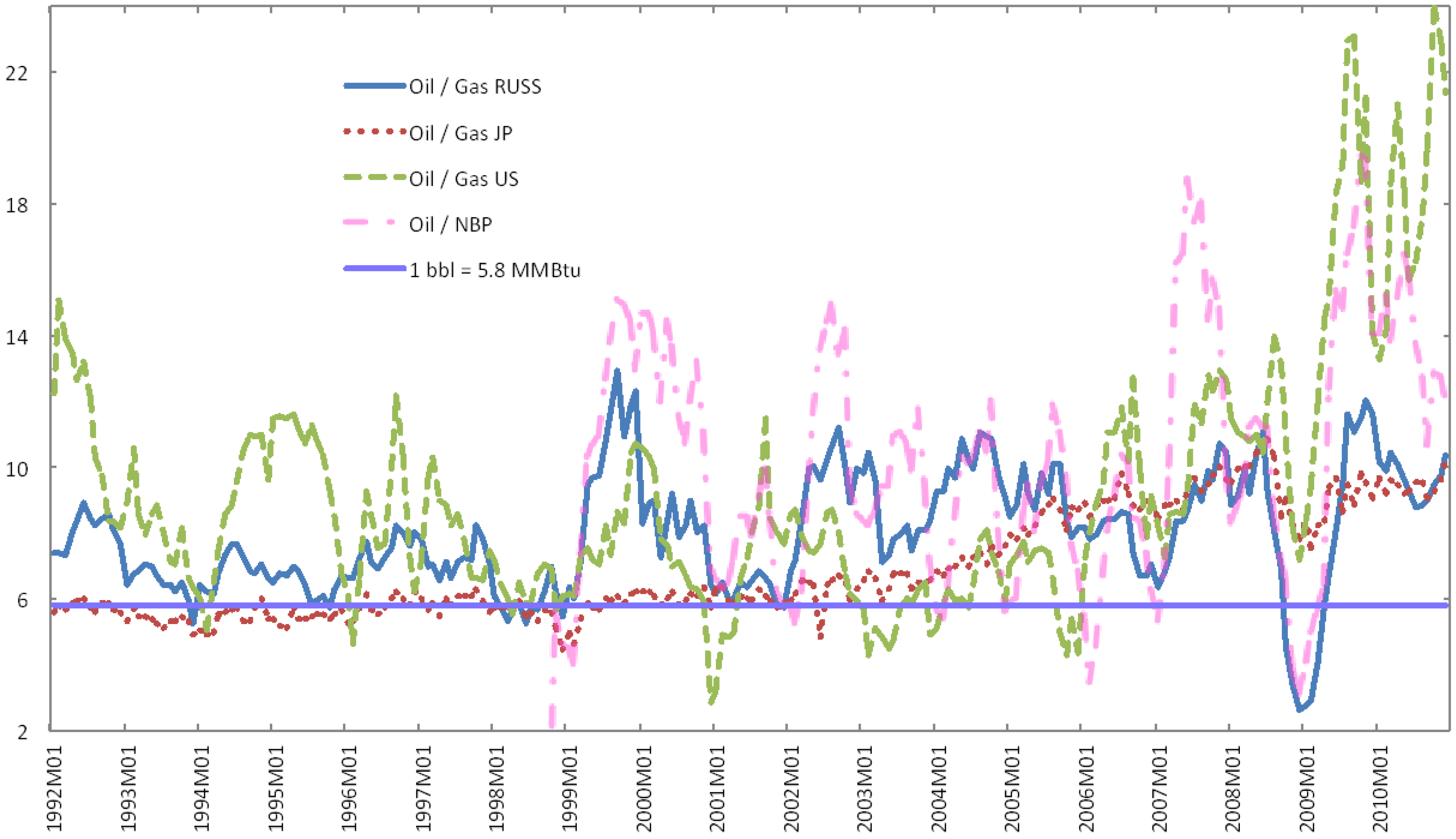
As shown in Figure 2, Russian natural gas was cheaper than oil in the investigated period, but the price ratio always eventually returned to the 5.8 equilibrium level. This is not surprising as the price of Russian natural gas is based on lagged fuel oil and gas oil futures prices. Thus, the ratio between the price of oil and the price of Russian natural gas in Figure 2 can divert from the 5.8 level because the crude oil price is used instead of refined oil product prices. The pricing formula of Russian gas keeps the price at, or close to, parity with crude oil. Russian gas may even be overpriced when crude oil enters a bear market; conversely, when crude is in a bull market, Russian natural gas is at a discount with respect to crude oil.

Figure 2. The Russian natural gas (bold line), Japanese LNG (dotted line), US natural gas (dashed line) and UK natural gas (dashed-dotted line) prices compared to crude oil price and thermal parity.

Figure 2. The Russian natural gas (bold line), Japanese LNG (dotted line), US natural gas (dashed line) and UK natural gas (dashed-dotted line) prices compared to crude oil price and thermal parity.

The Russian quarterly clearing gas prices are derived from fuel oil and the gasoil futures free on board (FOB) Mediterranean prices. The exact pricing formula varies by the contract, and the contractual terms, especially the constant part of the pricing equation, depend on the bargaining power of the importer. The general Russian pricing formula can be given in the form:

$$P_{g,RUSS}\left(t\right)=C+P_{g,RUSS}\left(t-1\right)\frac{1}{2}\left(\frac{\overline{F}\left(t\right)}{\overline{F}\left(t-1\right)}+\frac{\overline{G}\left(t\right)}{\overline{G}\left(t-1\right)}\right)$$

(1)

where P_g,RUSS(t) is the quarterly clearing price of Russian natural gas, C is the intercept of the regression, $\overline{F}\left(t\right)$ is the average price of fuel oil with less than 1% sulfur content in the last three quarters quoted in USD and $\overline{G}\left(t\right)$ is the average price of gas oil with less than 0.1% sulfur content in the last three quarters quoted in USD. Equation (1) is estimated by the Fully Modified Ordinary Least Squares (FMOLS) regression [22] since the oil and the Russian gas prices are cointegrated (see Table 2). The standard OLS would result in an asymptotic bias and non-Gaussian distribution in the parameter estimates due to super convergence of the estimator under cointegration. Since fuel oil and gas oil prices are closely related to crude oil prices, for the sake of simplicity these prices are substituted with crude prices and the equation is estimated in the form:

(2)

where ${\overline{P}}_{Oil}\left(t\right)$ is the average price of crude oil for the last three quarters quoted in USD and standard errors are in parentheses. The Russian gas price and the oil price are integrated in the order one (I(1)) (see Table 1). The estimated residuals are I(0), hence the dependent and independent variables are cointegrated, confirming the results in Table 2. The Wald test shows that the intercept is not significantly different from zero and the slope coefficient is not significantly different from unity. Therefore, it cannot be rejected that Equation (2) describes Russian natural gas prices.

We investigate whether the Russian gas price is underpriced with respect to current crude oil prices because in Equation (2) average oil prices for the preceding three quarters are used instead of current prices. The following regression is estimated:

$$\ln \frac{P_{g,RUSS}\left(t\right)}{{P^{\prime }}_{g,RUSS}\left(t\right)}=\widehat{\alpha }+{\displaystyle \sum _{k=0}^3{\widehat{\beta }}_k{r}_{Oil}}\left(t-k\right)+\widehat{\epsilon }\left(t\right)$$

(3)

where P’_g,RUSS(t) is a hypothetical Russian gas price assuming thermal parity with oil; that is,

(4)

where $r_{Oil}\left(t\right)$ is the log return of crude oil. The $\widehat{\alpha }$ is −0.004, which is not significantly different from zero. The estimated $\widehat{\beta }$ vector is (−0.986, 0.318, 0.417, 0.403), whose elements are significant at any usual level; the R² is 94.12%. The Wald test fails to reject that the intercept is zero and the beta vector is (−1.000, 0.333, 0.333, 0.333). This result indicates that lagged oil prices are exclusively and equally responsible for the departure from thermal parity.

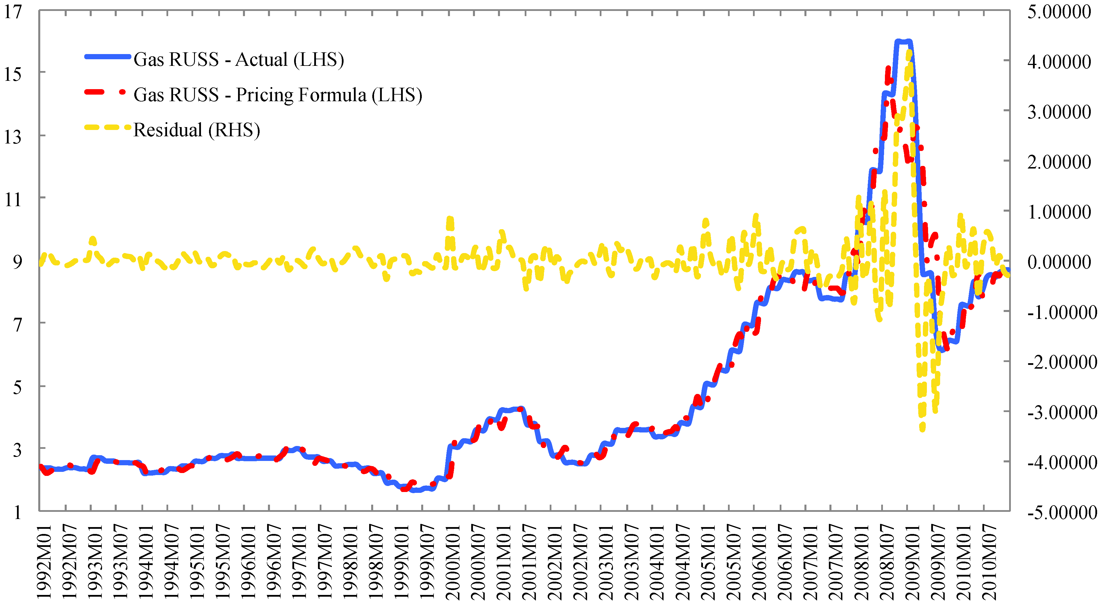
Figure 1 indicates that in the last few years of the dataset, although Russian gas prices follow the price developments of crude oil, the underpricing was much more severe and the pricing appeared to be more independent of crude oil. To test for the validity of Equation (2) Figure 3 shows the actual price of Russian natural gas as reported in the IMF database and the price which is forecast by Equation (2). In Figure 3 the residual of the forecast equation is also presented. There is no consistent deviation from the pricing formula; however, recently there were substantial temporary deviations, especially during the financial crisis. Russian gas exporters had to give concessions to European importers owing to competition from spot LNG trading.

Figure 3. The actual Russian natural gas price and the forecast price by Equation (2). Prices are measured on the left-hand side (LHS) in $/MMBtu and the residuals are measured on the right-hand side (RHS) in $/MMBtu.

Figure 3. The actual Russian natural gas price and the forecast price by Equation (2). Prices are measured on the left-hand side (LHS) in $/MMBtu and the residuals are measured on the right-hand side (RHS) in $/MMBtu.

3.2. The Japanese LNG

Japanese LNG was priced close to parity with crude oil from 1992 to 2002 as LNG was pegged to Japanese Crude Cocktail (JCC)[25]. Although the constant and the slope vary in time, Asian long-term contracts generally price LNG in the form:

(5)

where C is a constant, β is the slope, and P_o,JCC(t) is the price of JCC. P_g,LNG(t) and C are expressed in $/MMBtu, while P_o,JCC(t) is expressed in $/bbl. A slope of 0.1724 would price LNG at parity with crude oil [26,27]. In addition, there are two stylized inflexion points—one in the neighborhood of 50–60 $/bbl and another at approximately 80–100 $/bbl [26]. Below the lower inflexion point and over the upper inflexion point, the slope is flatter, hence LNG prices outside the interval of 50–100 $/bbl are less sensitive to crude oil prices. The LNG price curve is frequently called the S curve due to the inflexion points. Below the lower inflexion point LNG is priced with a mark-up with respect to crude oil. The lower inflexion point is enacted to protect producers from prices that are too low, as they have to face high initial investments such as building LNG terminals. On the contrary, importers have bargained for a higher inflexion point that results in underpricing and protects them when oil prices are high. The higher inflexion point was first introduced in 2002 when China entered the market with its Guangdong and Fujian projects [28]. The Guangdong formula induced a relatively lower price in an environment where crude oil was rising and there was a weaker link to oil prices [29]:

(6)

The Guangdong formula underprices natural gas by more than 45% against crude oil when oil is at 50 $/bbl and by almost 58% when crude is at 100 $/bbl. Figure 2 shows that after 2002 LNG is priced substantially lower than parity with crude oil. As oil and Japanese LNG prices are cointegrated (see Table 2) Equation (5) is estimated by FMOLS, the estimates are presented in the first row of Table 2. The results are significantly different from the Guangdong formula (Equation 6): the constant is lower, while the slope is higher than in the Chinese formula. This estimation considers that the coefficients in the pricing equation are constant independently from the price of crude oil. To include the two inflexion points let us define two dummy variables: D(P_JCC ≤ 35) is one if crude oil is equal to or below 35 $/bbl and is zero otherwise. D(P_JCC ≤ 100) is one if crude oil is equal to or above 100 $/bbl and is zero otherwise. The estimation for the S curve in the second row of Table 2. The null hypothesis that the two inflexion points are jointly zero can be rejected on the Wald test. Below 35 $/bbl, the slope is steeper, and above 100 $/bbl, the slope is flatter, thus we cannot document any evidence for the S curve because below the lower pivot point, the slope is not flatter but steeper. The estimated pricing formula suggests that LNG is priced at parity with crude oil at approximately 20 $/bbl, and it is overpriced below and underpriced above that level.

As Figure 2 demonstrates, LNG prices might have experienced one or more structural breaks between 1992 and 2010. It is quite noticeable that from 2002 onwards LNG became severely underpriced against crude oil. Therefore the pricing equation is re-estimated for the period 2002–2010; the results are shown in Table 3. The slope for the 2002–2010 period is not substantially but is significantly different from the slope estimated for the full sample. The intercept is higher for the 2002–2010 period and is not significantly different from the intercept in the Guangdong formula (Equation 6). The pivot points, which were highly significant for the full sample, are not significant for the truncated sample. The S curve limitation thus cannot be documented for the 2002–2010 period, and the slope of the pricing formula is flat.

We also ran a regression on the pricing formula for the post-2005 period as the ECS report [28] argues that after 2005 Guangdong formula was renegotiated because the LNG market tightened significantly (see Table 3). The estimates for the 2005–2010 period are not significantly different from the estimated parameters for the 2002–2010 period. The lower inflexion point is excluded because during this period, oil prices were never at or below 35 $/bbl. Therefore we can document only one significant shift in the pricing regime, which occurred when China entered the market in 2002. As a robustness check, the pricing formula is also estimated for 1992–2001 (see Table 3). The pre-2002 estimation can confirm that the pricing formula was significantly different before and after 2002. The constant is only one-third of the constant for the post-2002 period and the slope is higher by 78%. Before 2002 LNG was thus priced at parity with crude oil when oil was approximately 20 $/bbl. Between 1992 and 2001 crude prices averaged 19 $/bbl, which means that LNG was overpriced by 1% on average (see also Figure 2). Thus, LNG was priced close to parity with crude oil before but not after China entered the market. Between 2002 and 2010 LNG was underpriced, since oil prices were upward oriented, the constant of the pricing formula was raised and the slope was lowered. Therefore the Guangdong project was successful in protecting importers from rising crude oil prices as LNG prices became less sensitive to oil prices.

Table 3. Fully modified OLS estimates of LNG prices.

	R²	C	Oil	Oil*D(PJCC ≤ 35)	Oil*D(PJCC ≥ 100)
1992–2010	0.9816	1.7650	0.0843
		(0.0710)	(0.0016)
	0.9861	1.1436	0.0938	0.0217	−0.0082
		(0.1425)	(0.0023)	(0.0048)	(0.0023)
2002–2010	0.9809	2.1198	0.0790
		(0.0614)	(0.0010)
	0.9807	2.1097	0.0793	0.0012	−0.0020
		(0.1236)	(0.0019)	(0.0031)	(0.0013)
2005–2010	0.9686	1.9831	0.0806
		(0.0805)	(0.0011)
	0.9689	2.0144	0.0805		−0.0018
		(0.1603)	(0.0024)		(0.0014)
1992–2001	0.9608	0.6415	0.1406
		(0.0870)	(0.0044)

This table shows the FMOLS (Fully Modified OLS) estimates of the LNG pricing equation.

Table 3. Fully modified OLS estimates of LNG prices.

	R²	C	Oil	Oil*D(PJCC ≤ 35)	Oil*D(PJCC ≥ 100)
1992–2010	0.9816	1.7650	0.0843
		(0.0710)	(0.0016)
	0.9861	1.1436	0.0938	0.0217	−0.0082
		(0.1425)	(0.0023)	(0.0048)	(0.0023)
2002–2010	0.9809	2.1198	0.0790
		(0.0614)	(0.0010)
	0.9807	2.1097	0.0793	0.0012	−0.0020
		(0.1236)	(0.0019)	(0.0031)	(0.0013)
2005–2010	0.9686	1.9831	0.0806
		(0.0805)	(0.0011)
	0.9689	2.0144	0.0805		−0.0018
		(0.1603)	(0.0024)		(0.0014)
1992–2001	0.9608	0.6415	0.1406
		(0.0870)	(0.0044)

This table shows the FMOLS (Fully Modified OLS) estimates of the LNG pricing equation.

3.3. US Henry Hub Natural Gas Prices

In the full sample period the HH benchmark was the most underpriced with respect to WTI (see Table 1). Before 2006, the natural gas to oil price ratio reverted to parity level approximately every two years. Although after 2006 the ratio did not revert to the parity level, before 2009, the underpricing of HH was not unusual based on the performance of the ratio in the preceding 17 years. Conversely, after 2009, it seems there was barely a connection between HH and crude oil prices, which is striking considering that the two fuels are substitutes.

First, a pricing equation that considers a similar pricing to that of LNG in the first row of Table 3 is tested in the form:

$$\begin{array}{c}{P}_{g,US}\left(t\right)=1.515\hspace{0.17em}\hspace{0.17em}+\hspace{0.17em}\hspace{0.17em}0.071P_{Oil}\left(t\right)+\widehat{\epsilon }\left(t\right)\\ \hspace{0.17em}\hspace{0.17em}\hspace{0.17em}\hspace{0.17em}\hspace{0.17em}\hspace{0.17em}\hspace{0.17em}\hspace{0.17em}\hspace{0.17em}\hspace{0.17em}\hspace{0.17em}\hspace{0.17em}\hspace{0.17em}\hspace{0.17em}\hspace{0.17em}\hspace{0.17em}\hspace{0.17em}\hspace{0.17em}\hspace{0.17em}\hspace{0.17em}\hspace{0.17em}\hspace{0.17em}\hspace{0.17em}\hspace{0.17em}\hspace{0.17em}\hspace{0.17em}\hspace{0.17em}\hspace{0.17em}\hspace{0.17em}\hspace{0.17em}\hspace{0.17em}\hspace{0.17em}\hspace{0.17em}\hspace{0.17em}\hspace{0.17em}\hspace{0.17em}\left(0.491\right)\hspace{0.17em}\hspace{0.17em}\hspace{0.17em}\left(0.011\right)\hspace{0.17em}\hspace{0.17em}\hspace{0.17em}\hspace{0.17em}\hspace{0.17em}\hspace{0.17em}\hspace{0.17em}\hspace{0.17em}\hspace{0.17em}\hspace{0.17em}\hspace{0.17em}\hspace{0.17em}\hspace{0.17em}\hspace{0.17em}\hspace{0.17em}\hspace{0.17em}\hspace{0.17em}\hspace{0.17em}\hspace{0.17em}\hspace{0.17em}\hspace{0.17em}\hspace{0.17em}\hspace{0.17em}\hspace{0.17em}\hspace{0.17em}\hspace{0.17em}\hspace{0.17em}\hspace{0.17em}\hspace{0.17em}\hspace{0.17em}\hspace{0.17em}\hspace{0.17em}\hspace{0.17em}\hspace{0.17em}\hspace{0.17em}\hspace{0.17em}\hspace{0.17em}\hspace{0.17em}\hspace{0.17em}\hspace{0.17em}\hspace{0.17em}\hspace{0.17em}\hspace{0.17em}\end{array}$$

(7)

where the R² is 53.91% and standard errors are in parentheses. Although HH is not cointegrated with crude oil (see Table 2), the residuals of the FMOLS regression are stationary, hence the estimated parameters of Equation (7) are unbiased [30]. The estimation suggests that US gas price is underpriced if oil is above 15 $/bbl. Equation (7) induces more severe underpricing for US gas prices than the pricing formulas estimated for LNG (see Table 3). The Wald test with a null that Equation (7) matches the estimated LNG pricing formula for the period 1992–2010 can be rejected at a 95% level. HH is thus priced on a different basis than LNG; however, the two formulas are similar.

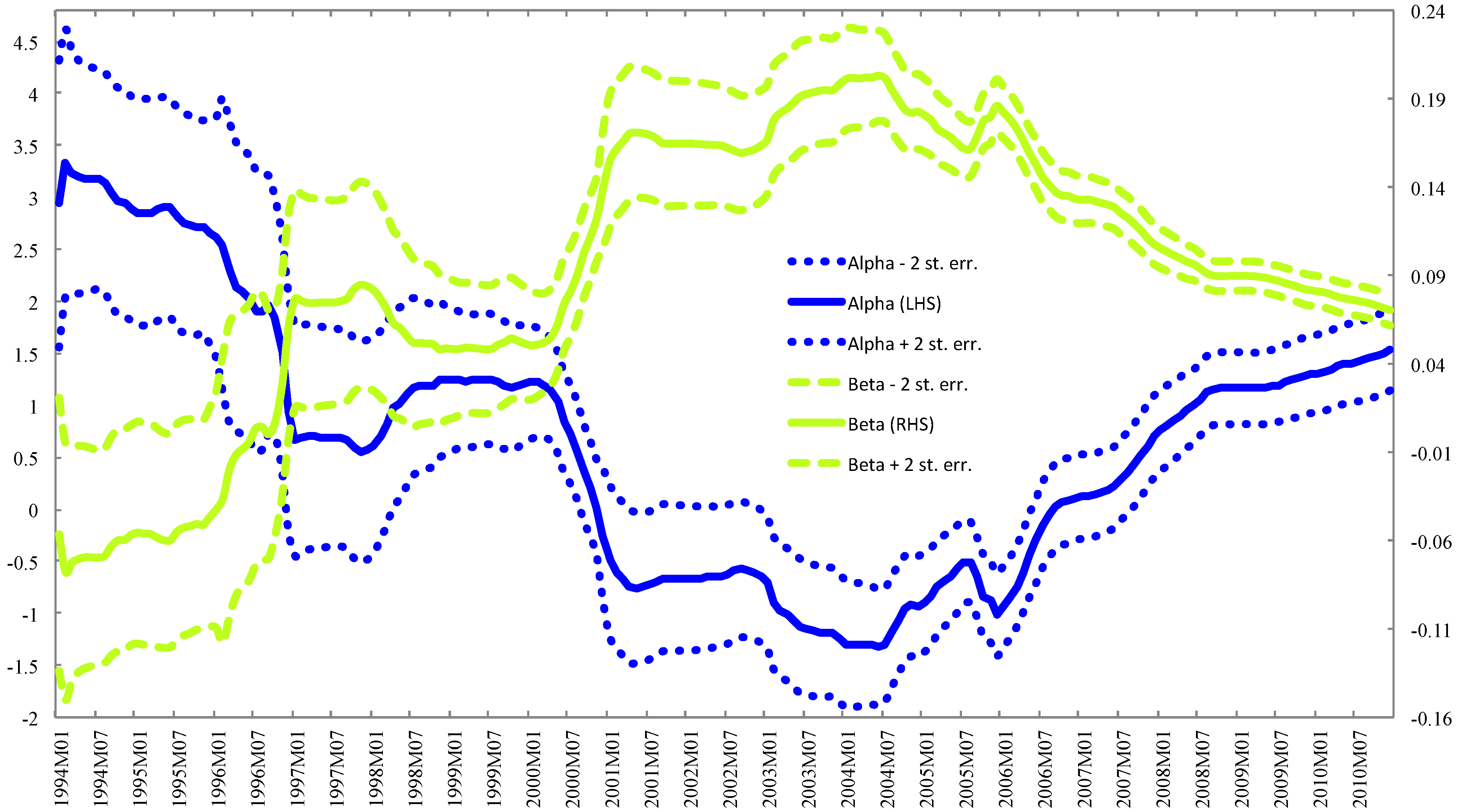
Figure 2 prompts us to investigate the stability of the parameter estimates in Equation (7). Therefore recursive OLS estimates of the intercept and the slope are plotted in Figure 4. The lower explanatory power of Equation (7) can be at least partly explained by the time-varying nature of the relationship between HH and oil prices [31]. Until 2001 the recursive estimates show a gradual strengthening in the oil-gas price relationship that was relatively stable until 2006 when it started to weaken.

Figure 4. The recursive OLS estimates of the regression of Henry Hub natural gas prices on oil prices. On the left-hand side (LHS), the intercept of the regression is measured in dollars per million British thermal unit (MMBtu), and on the right-hand side (RHS), the slope (beta) is measured in MMBtu per barrel. The plus/minus two standard error bands are also presented for both estimates.

Figure 4. The recursive OLS estimates of the regression of Henry Hub natural gas prices on oil prices. On the left-hand side (LHS), the intercept of the regression is measured in dollars per million British thermal unit (MMBtu), and on the right-hand side (RHS), the slope (beta) is measured in MMBtu per barrel. The plus/minus two standard error bands are also presented for both estimates.

4. Causality Links between Natural Gas Benchmark Prices

Although the oil link in both Japanese LNG and Russian gas prices was weaker in the second part of the sample period, and especially after 2002 in the case of LNG, and during 2008–2009 in the case of Russian gas price, they were still linked to oil prices, whereas after 2006 oil had a significantly inferior explanatory power in US gas prices. Therefore, it is worth subjecting the oil price—US natural gas price relationship and the relations of US gas prices to other benchmarks to further investigation. In Table 4, the results of pairwise Granger causality tests are presented. Vector error correction (VEC) models are estimated for those price pairs that appeared cointegrated in Table 2 and vector autoregression (VAR) models for the log difference of those pairs that are not cointegrated. The Granger tests are performed as block exogenity Wald tests. The lag selection is based on the Schwarz information criterion and when there is significant autocorrelation in the residuals we add further lags to the VECs/VARs. Oil price Granger causes all the gas benchmarks in Panel A and for a shorter period in Panel B that includes also NBP. However, the reverse Granger causality link cannot only be rejected between Japanese LNG and oil prices at the 5% level. Japanese LNG prices are linear function of crude oil prices (see Table 3), hence the mutual Granger causality between crude prices and LNG prices is not striking. Furthermore, for the same reason LNG prices Granger cause the other gas benchmarks; the only exception is NBP (Table 3, Panel B). Conversely, Russian gas prices are determined by lagged oil prices, thus the Granger causality link from Russian gas prices to oil prices and Japanese LNG prices can be rejected. Russian gas prices, however, Granger cause NBP and US gas prices, albeit the latter only in the full sample period. Similarly, the Granger causality from NBP to Russian gas prices cannot be rejected. The strong association between the two European benchmarks is not surprising as the Interconnector that integrates the UK gas market with the continental European market allows gas flow in either direction depending on gas prices in the UK and on the continent. Since LNG is priced on current oil prices, it seems sensible that US gas prices neither Granger cause oil prices, nor LNG prices. The Granger causality links from US gas prices to European gas benchmarks are, however, more interesting. In the full sample period the Granger causality from US gas prices to Russian gas prices cannot be rejected. Conversely, if we concentrate only on the period of October 1998–December 2010 the causality link between the US and Russian gas prices disappears. Furthermore, data are available for NBP in this shorter time period and the Granger test rejects a Granger causality link from US gas prices to NBP prices. Thus, it seems in the second part of the data that the strong mutual causality link between US and European gas prices ceased.

Granger causality tests have thus confirmed our conjecture that in the second part of the data, US gas is priced more independently from oil, which results in a less connected global gas market. In addition, gas benchmarks in Europe and Asia remained dependent on crude oil price.

Table 4. Pairwise Granger causality tests.

Panel A (January 1992–December 2010)
	Chi Sqr. Statistic	p-Value	VAR/VEC
Oil does not Granger Cause Gas JP	35.979	0.000	VEC
Gas JP does not Granger Cause Oil	22.692	0.001
Oil does not Granger Cause Gas RUSS	29.212	0.000	VEC
Gas RUSS does not Granger Cause Oil	3.401	0.334
Oil does not Granger Cause Gas US	16.603	0.011	VAR
Gas US does not Granger Cause Oil	4.752	0.576
Gas JP does not Granger Cause Gas RUSS	29.364	0.000	VEC
Gas RUSS does not Granger Cause Gas JP	1.529	0.822
Gas JP does not Granger Cause Gas US	28.623	0.004	VAR
Gas US does not Granger Cause Gas JP	15.024	0.240
Gas US does not Granger Cause Gas RUSS	19.112	0.024	VAR
GAS RUSS does not Granger Cause Gas US	17.280	0.045
Panel B (October 1998–December 2010)
Oil does not Granger Cause Gas JP	10.358	0.035	VEC
Gas JP does not Granger Cause Oil	12.876	0.012
Oil does not Granger Cause Gas RUSS	44.600	0.000	VEC
Gas RUSS does not Granger Cause Oil	1.971	0.741
Oil does not Granger Cause Gas US	21.866	0.009	VAR
Gas US does not Granger Cause Oil	13.374	0.146
	Chi Sqr. Statistic	p-Value	VAR/VEC
Oil does not Granger Cause NBP	20.150	0.043	VEC
NBP does not Granger Cause Oil	17.352	0.098
Gas JP does not Granger Cause Gas RUSS	31.408	0.000	VEC
Gas RUSS does not Granger Cause Gas JP	1.091	0.779
Gas JP does not Granger Cause Gas US	16.900	0.050	VAR
Gas US does not Granger Cause Gas JP	13.991	0.123
Gas JP does not Granger Cause NBP	12.207	0.142	VEC
NBP does not Granger Cause Gas JP	15.335	0.053
GAS RUSS does not Granger Cause Gas US	10.122	0.120	VAR
Gas US does not Granger Cause Gas RUSS	9.266	0.159
Gas RUSS does not Granger Cause NBP	13.717	0.033	VEC
NBP does not Granger Cause Gas RUSS	14.306	0.026
Gas US does not Granger Cause NBP	9.692	0.084	VEC
NBP does not Granger Cause Gas US	9.998	0.075

This table shows pairwise Granger causality tests between oil, Japanese LNG, Russian and US natural gas prices for the period 1992–2010 in Panel A. Panel B expands the analysis with NBP prices for the period October 1998–December 2010.

Table 4. Pairwise Granger causality tests.

Panel A (January 1992–December 2010)
	Chi Sqr. Statistic	p-Value	VAR/VEC
Oil does not Granger Cause Gas JP	35.979	0.000	VEC
Gas JP does not Granger Cause Oil	22.692	0.001
Oil does not Granger Cause Gas RUSS	29.212	0.000	VEC
Gas RUSS does not Granger Cause Oil	3.401	0.334
Oil does not Granger Cause Gas US	16.603	0.011	VAR
Gas US does not Granger Cause Oil	4.752	0.576
Gas JP does not Granger Cause Gas RUSS	29.364	0.000	VEC
Gas RUSS does not Granger Cause Gas JP	1.529	0.822
Gas JP does not Granger Cause Gas US	28.623	0.004	VAR
Gas US does not Granger Cause Gas JP	15.024	0.240
Gas US does not Granger Cause Gas RUSS	19.112	0.024	VAR
GAS RUSS does not Granger Cause Gas US	17.280	0.045
Panel B (October 1998–December 2010)
Oil does not Granger Cause Gas JP	10.358	0.035	VEC
Gas JP does not Granger Cause Oil	12.876	0.012
Oil does not Granger Cause Gas RUSS	44.600	0.000	VEC
Gas RUSS does not Granger Cause Oil	1.971	0.741
Oil does not Granger Cause Gas US	21.866	0.009	VAR
Gas US does not Granger Cause Oil	13.374	0.146
	Chi Sqr. Statistic	p-Value	VAR/VEC
Oil does not Granger Cause NBP	20.150	0.043	VEC
NBP does not Granger Cause Oil	17.352	0.098
Gas JP does not Granger Cause Gas RUSS	31.408	0.000	VEC
Gas RUSS does not Granger Cause Gas JP	1.091	0.779
Gas JP does not Granger Cause Gas US	16.900	0.050	VAR
Gas US does not Granger Cause Gas JP	13.991	0.123
Gas JP does not Granger Cause NBP	12.207	0.142	VEC
NBP does not Granger Cause Gas JP	15.335	0.053
GAS RUSS does not Granger Cause Gas US	10.122	0.120	VAR
Gas US does not Granger Cause Gas RUSS	9.266	0.159
Gas RUSS does not Granger Cause NBP	13.717	0.033	VEC
NBP does not Granger Cause Gas RUSS	14.306	0.026
Gas US does not Granger Cause NBP	9.692	0.084	VEC
NBP does not Granger Cause Gas US	9.998	0.075

This table shows pairwise Granger causality tests between oil, Japanese LNG, Russian and US natural gas prices for the period 1992–2010 in Panel A. Panel B expands the analysis with NBP prices for the period October 1998–December 2010.

5. Conclusions

We have investigated the price formation of international natural gas markets and their relationships with each other and the global crude oil market. The relationship between oil and gas markets depends on the natural gas market and it varies over time. In the first half of the sample period, from 1992 to 2001, natural gas markets were strongly related to the oil market, and over a longer time period oil-to-gas prices always reverted to the thermal parity level. In the second half of the dataset, from 2002 to 2010, natural gas was more severely underpriced with respect to crude oil and the relationship between oil and natural gas markets became weaker.

Russian natural gas is related to crude oil during the entire sample period. However, Russian export prices have recently also shown some early signs that pricing may become more independent from oil. Similarly, Japanese LNG prices were influenced less by crude oil prices in the second half of the dataset. LNG pricing changed around 2002 due to the market entrance of China, which could bargain for a lower LNG price in an environment of rising oil prices. The LNG prices have remained derivable from crude oil prices, but the constant has become more important, whereas the sensitivity to crude oil price became less important in determining the price. The change in the pricing formula coupled with rising crude prices and resulted in more severe LNG underpricing against crude oil.

US natural gas prices do not show such a strong relationship to crude oil prices, as Russian export prices, NBP prices or Japanese LNG prices. Recursive OLS estimates and Granger causality tests show that the relationship between US natural gas and crude oil prices has recently relaxed substantially. As the other two benchmarks remained indexed on crude oil price, the US benchmark price exhibited departures from the European and Asian prices. Thus, at the current stage, a globally integrated natural gas market, similar to the global oil market, has not evolved. The main natural gas markets, however, exhibit some level of integration as the cointegration tests and Granger causality tests show.

References and Notes

- BP Statistical Review of World Energy, 2001–2011; BP P.L.C.: London, UK, 2011.
- Energy Sector Inquiry; European Commission—DG Competition: Brussels, Belgium, 2007.
- Davoust, R. Gas Price Formation, Structure and Dynamics. Institut Francais des Relations Internationales; Working Paper; IFRI: Paris, France, 2008. [Google Scholar]
- Villar, J.A.; Joutz, F.L. The Relationship between Crude Oil and Natural Gas Prices; Energy Information Agency, Office of Oil and Gas, Administration Manuscript; EIA: Washington, DC, USA, 2006. [Google Scholar]
- Green, D.J. A small scale, partial equilibrium model of natural gas markets: Responses to alternative deregulation scenarios and oil price changes. South. Econ. J. 1984, 50, 1112–1130. [Google Scholar] [CrossRef]
- Ashe, F.; Osmundsen, P.; Sandsmark, M. Is It All Oil? CESIFO Working Paper No. 1401; CESifo: Munich, Germany, 2005. [Google Scholar]
- Siliverstovs, B.; L’Hégaret, G.; Neumannc, A.; von Hirschhausen, C. International market integration for natural gas? A cointegration analysis of prices in Europe, North America and Japan. Energy Econ. 2005, 27, 603–615. [Google Scholar]
- The correlation coefficients between the returns of Oman, Qatar and Dubai near month futures are all higher than 0.99, thus all these prices could stand as a benchmark for middle eastern oil.
- The recent Brent premium over WTI can somewhat challenge this view.
- Smith, K. Russian Energy Pressure Fails to Unite Europe; Center for Strategic and International Studies (CSIS): Washington, DC, USA, 2007. [Google Scholar]
- Smith, K. Putin Checkmates Europe’s Energy Hopes; Center for Strategic and International Studies (CSIS) Commentary: Washington, DC, USA, 2007. [Google Scholar]
- Harmsen, R.; Jepma, C. North West European gas market: Integrated already. 2011. Available online: http://www.europeanenergyreview.eu/index.php?id=2695 (accessed on 18 October 2012).
- Platts daily spot LNG Price assessments. 2010. Available online: http://www.platts.com/IM.Platts.Content/downloads/faqs/lngfaq.pdf (accessed on 18 October 2012).
- World Energy Outlook; OECD/IEA: Paris, France, 2010.
- Lee, W.W. US lessons for energy industry restructuring: Based on natural gas and California electricity incidences. Energy Policy 2004, 32, 237–259. [Google Scholar] [CrossRef]
- Welch, B.L. On the comparison of several mean values: An alternative approach. Biometrika 1951, 38, 330–336. [Google Scholar] [CrossRef]
- Dickey, D.A.; Fuller, W.A. Distribution of the estimators for autoregressive time series with a unit root. J. Am. Stat. Assoc. 1979, 74, 427–431. [Google Scholar]
- Phillips, P.C.B.; Perron, P. Testing for a unit root in time series regression. Biometrika 1988, 75, 335–346. [Google Scholar] [CrossRef]
- Kwiatkowski, D.; Phillips, P.C.B.; Schmidt, P.; Shin, Y. Testing the null hypothesis of stationary against the alternative of a unit root. J. Econ. 1992, 54, 159–178. [Google Scholar] [CrossRef]
- Lo, A.W.; MacKinlay, A.C. Stock market prices do not follow random walks: Evidence from a simple specification test. Rev. Financ. Stud. 1988, 1, 41–66. [Google Scholar] [CrossRef]
- Cochrane, J.H. How big is the random walk in GNP? J. Polit. Econ. 1988, 96, 893–920. [Google Scholar] [CrossRef]
- Kao, C.W.; Wan, J.Y. Information transmission and market interactions across the Atlantic—An empirical study on the natural gas market. Energy Econ. 2009, 31, 152–161. [Google Scholar] [CrossRef]
- Hayes, M.H. Flexible LNG Supply, Storage and Price Formation in a Global Natural Gas Market. Ph.D. Thesis, Stanford University, Stanford, CA, USA, 2006. [Google Scholar]
- Neumann, A. Linking natural gas markets—Is LNG doing its job? Energy J. 2009, 30, 187–200. [Google Scholar] [CrossRef]
- The abbreviation officially stands for Japan Customs-cleared Crude (JCC), which is the average price of the customs-cleared crude oil imports into Japan (formerly the average of the top twenty crudes by volume) as reported in Japanese customs statistics. It is nicknamed the “Japanese Crude Cocktail”.
- Eng, G. A Formula for LNG Pricing; A Report Prepared for the Ministry of Economic Development: Wellington, New Zealand, 2008. Available online: http://www.med.govt.nz/templates/MultipageDocumentTOC____39562.aspx (accessed on 14 March 2012).
- The BP Statistical Review of World Energy; BP P.L.C.: London, UK, 2008; p. 44.
- Fostering LNG Trade: Developments in LNG Trade and Pricing; Energy Charter Secretariat: Brussels, Belgium, 2009.
- Eng, G. A Formula for LNG Pricing; A Report Prepared for the Ministry of Economic Development: Wellington, New Zealand, 2006. Available online: http://www.med.govt.nz/upload/42265/LNG%20Pricing%20Formula.pdf (accessed on 14 March 2012).
- Since the results of unit root tests are ambiguous (see Table 1), it may be that oil and natural gas prices are both integrated at order zero, which induces stationary residuals.
- Recursive OLS estimates for the Russian pricing formula are stable. The recursive estimates for LNG prices confirm regime change in 2002 (Table 2). These results are not presented here for space saving reasons, but they are available upon request.
© 2012 by the authors; licensee MDPI, Basel, Switzerland. This article is an open access article distributed under the terms and conditions of the Creative Commons Attribution license (http://creativecommons.org/licenses/by/3.0/).
Share and Cite
MDPI and ACS Style
Erdős, P.; Ormos, M. Natural Gas Prices on Three Continents. Energies 2012, 5, 4040-4056. https://doi.org/10.3390/en5104040
AMA Style
Erdős P, Ormos M. Natural Gas Prices on Three Continents. Energies. 2012; 5(10):4040-4056. https://doi.org/10.3390/en5104040
Chicago/Turabian StyleErdős, Péter, and Mihály Ormos. 2012. "Natural Gas Prices on Three Continents" Energies 5, no. 10: 4040-4056. https://doi.org/10.3390/en5104040