An Integrated Multi-Criteria Decision Making Model for Evaluating Wind Farm Performance


Abstract
:1. Introduction
2. Methodologies
2.1. Interpretive Structural Modeling (ISM)

| Authors | Theories or Applications |
|---|---|
| Sahney et al. [12] | To propose an integrated framework for quality in education by applying SERVQUAL, quality function deployment, ISM and path analysis. |
| Agarwal et al. [13] | To understand the characteristics and interrelationship of variables in an agile supply chain. |
| Thakkar et al. [14] | To develop a balanced scorecard (BSC) framework using cause and effect analysis, ISM and ANP for performance measurement. |
| Faisal et al. [15] | To employ ISM to identify various information risks that could impact a supply chain and to present a risk index to quantify information risks. |
| Kannan and Haq [16] | To understand the interactions of criteria and sub-criteria that are used to select the supplier for the built-in-order supply chain environment. |
| Qureshi et al. [17] | To model the logistics outsourcing relationship variables to enhance shippers’ productivity and competitiveness in logistical supply chain. |
| Singh et al. [18] | To construct a structural relationship of critical success factors for implementing advanced manufacturing technologies. |
| Upadhyay et al. [19] | To use content analysis, nominal group technique (NGT) and ISM to develop a hierarchy framework for quality engineering education. |
| Thakkar [20] | To propose an integrated mathematical approach based on ISM and graph theoretic matrix for evaluating buyer-supplier relationships. |
| Vivek et al. [21] | To establish changing emphasis of the core, transactional and relational specificity constructs in offshoring alliances. |
| Yang et al. [22] | To study the relationships among the sub-criteria and use integrated fuzzy MCDM techniques to study the vendor selection problem. |
| Wang et al. [23] | To analyze the interactions among the barriers to energy-saving projects in China. |
| Chidambaranathan et al. [24] | To develop the structural relationship among supplier development factors and to define the levels of different factors based on their dependence power and mutual relationships. |
| Kannan et al. [25] | To construct a multi-criteria group decisionmaking (MCGDM) model through ISM and fuzzy technique for order preference by similarity to ideal solution (TOPSIS) to guide the selection process of best third-party reverse logistics providers. |
| Mukherjee and Mondal [26] | To examine relevant issues in managing the remanufacturing technology for an Indian company. |
| Feng et al. [27] | To propose a hybrid fuzzy integral decision-making model, which integrates factor analysis, ISM, Markov chain, fuzzy integral and the simple additive weighted method, for selecting locations of high-tech manufacturing centers. |
| Lee et al. [28] | To determine the interrelationship among the critical factors for technology transfer of new equipment in high technology industry and apply the FANP to evaluate the technology transfer performance of equipment suppliers. |
| Lee et al. [29] | To determine the interrelationship among the criteria in a conceptual model to help analyze suitable strategic products for photovoltaic silicon thin-film solar cell power industry. |
| Lee et al. [30] | To propose an integrated model, which applies ISM to understand the interrelationship among criteria, for evaluating various technologies for a flat panel manufacturer. |
2.2. Fuzzy Analytic Network Process (FANP)
- Decompose the problem into a network. The overall objective is in the first level. The second level includes criteria, and there might be sub-criteria under each criterion. The dependences and feedback among criteria and among sub-criteria are considered. The last level includes the alternatives that are under evaluation.
- Prepare a questionnaire based on the constructed network, and ask experts to fill out the questionnaire. Consistency index and consistency ratio for each comparison matrix are calculated to examine the consistency of each expert’s judgment [31]. If the consistency test is not passed, the original values in the pairwise comparison matrix must be revised by the expert.
- Transform the scores of pairwise comparison into fuzzy numbers.
- Aggregate the results from Step 3. The fuzzy positive reciprocal matrix can be defined as:where: : a positive reciprocal matrix of decision maker k;
- : relative importance between decision elements i and j;
- and .
- Defuzzy the synthetic trapezoid fuzzy numbers into crisp numbers.
- Form pairwise comparison matrices using the defuzzificated values, and calculate priority vector for each pairwise comparison matrix.where is the matrix of pairwise comparison, w is the eigenvector, and is the largest eigenvalue of .
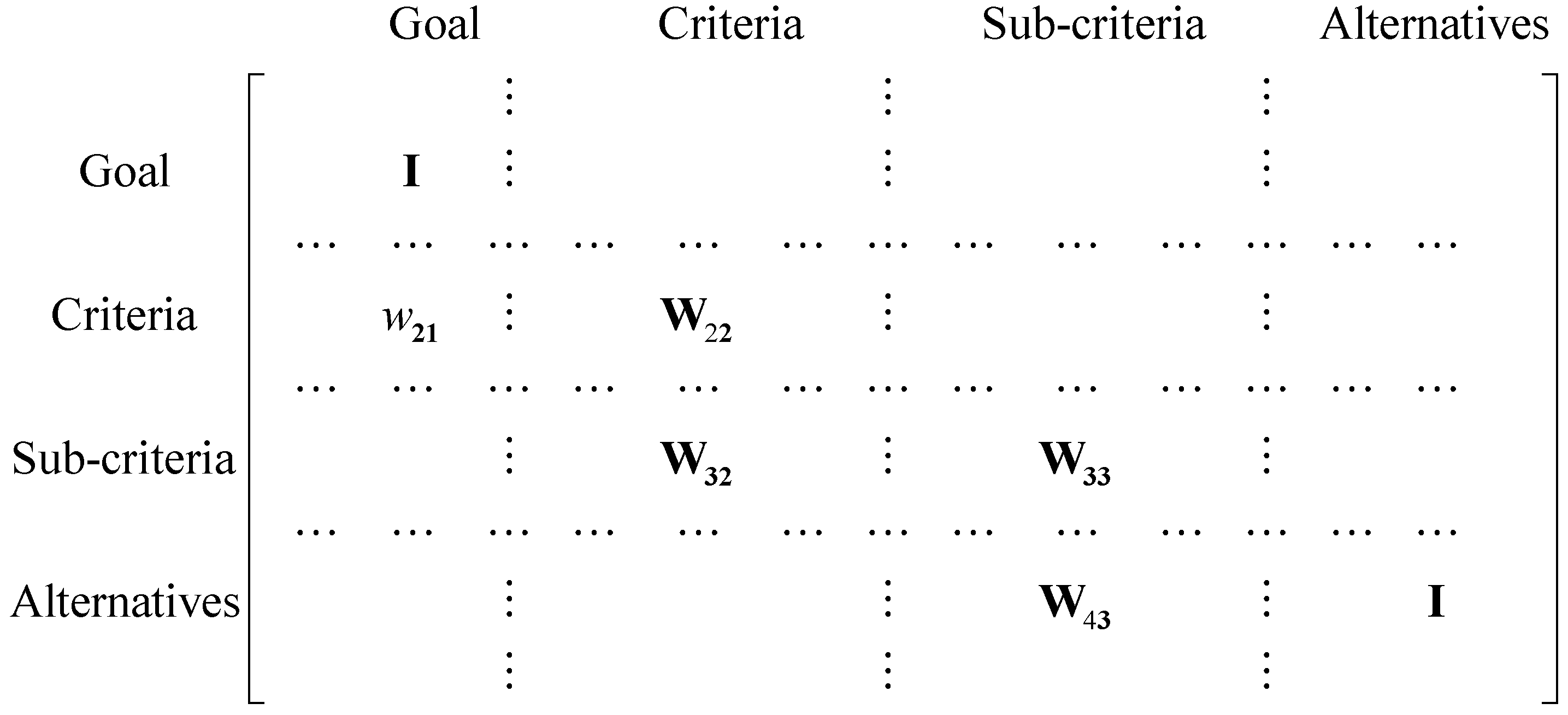
- Form an unweighted supermatrix, as shown in Figure 1.
- Form a weighted supermatrix to ensure column stochastic.
- Calculate the limit supermatrix by taking the weighted supermatrix to powers so that the supermatrix converges into a stable supermatrix. Obtain the priority weights of the alternatives from the limit supermatrix.

2.3. Benefits, Opportunities, Costs and Risks (BOCR)
- Additive:where Bi, Oi, Ci and Ri represent respectively the synthesized results of alternative i under merit B, O, C and R, and b, o, c and r are respectively normalized weights of merit B, O, C and R.Pi = bBi + oOi + c[(1/Ci)Normalized] + r[(1/Ri)Normalized]
- Probabilistic additive:Pi = bBi + oOi + c(1 − Ci) + r(1 − Ri)
- Subtractive:Pi = bBi + oOi − cCi − rRi
- Multiplicative priority powers:Pi = Bib Oio [(1/Ci)Normalized]c [(1/Ri)Normalized]r
- Multiplicative:Pi = BiOi/CiRi
3. An Integrated Model for Evaluating Wind Farm Performance
- Step 1. Form a committee of experts in the wind farm industry to define the wind farm evaluation problem.
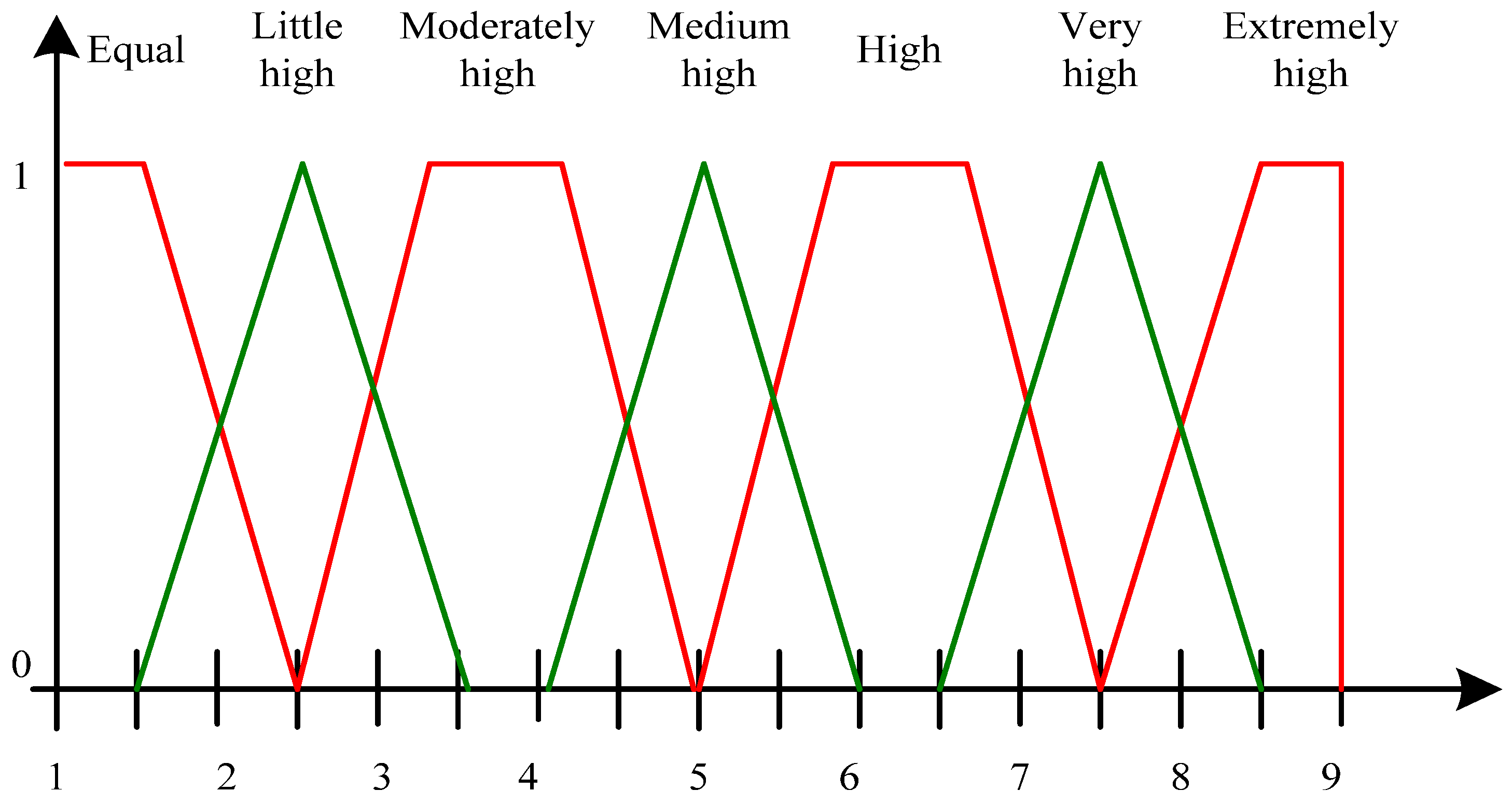
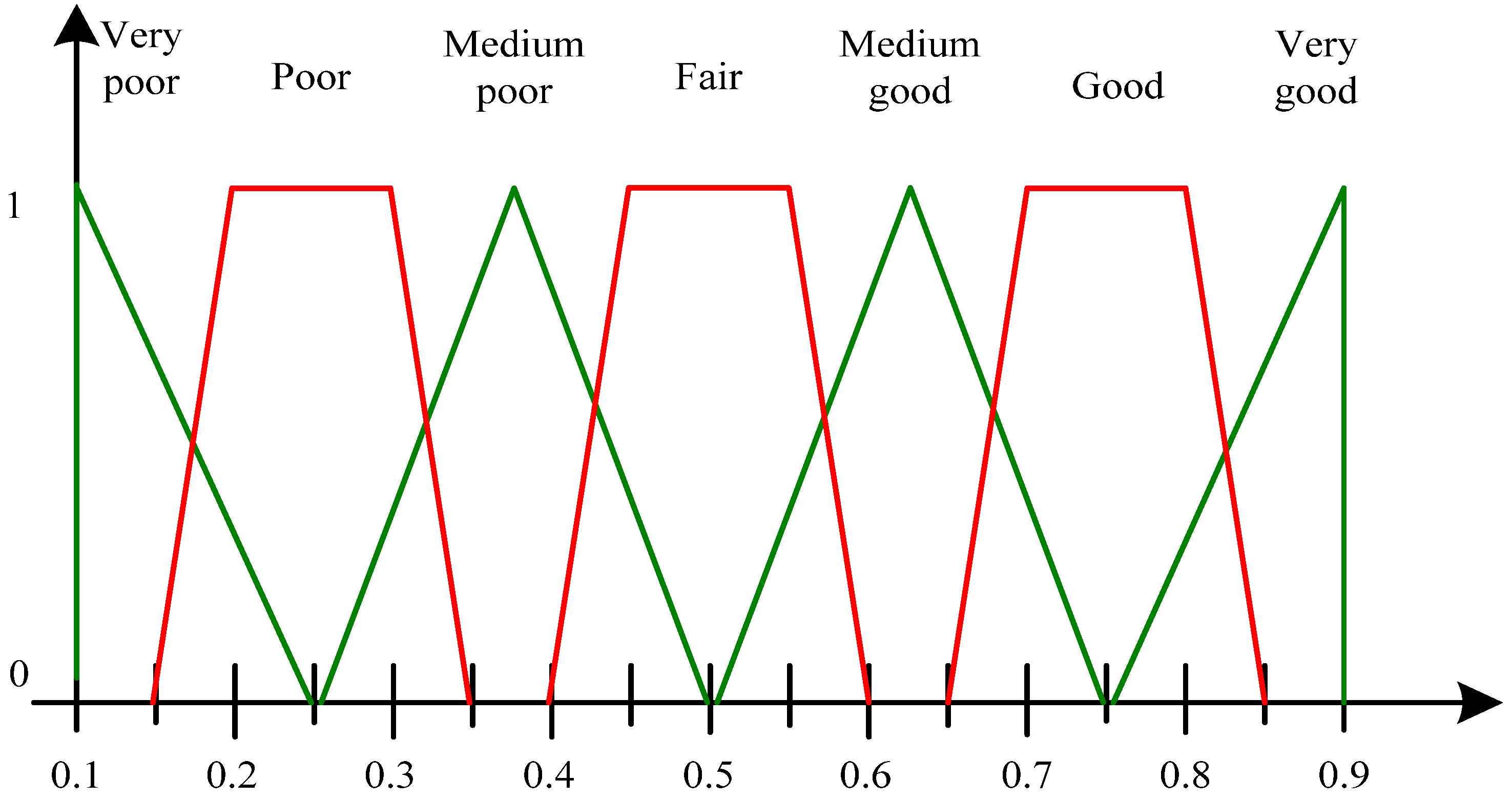
- Step 3. Prepare a questionnaire to collect experts’ opinions based on the control network. Experts are asked to pairwise compare the strategic criteria using seven different linguistic terms, as depicted in Figure 3. The linguistic variables of pairwise comparison of each part of the questionnaire from each expert are transformed into trapezoid fuzzy numbers. Experts are also asked to determine the ranking of each merit (B, O, C, R) on each strategic criterion by a seven-step scale, as depicted in Figure 4.Figure 3. Membership function of fuzzy numbers for relative importance/performance.
![Energies 04 02002 g003]() Figure 4. Membership function of fuzzy numbers for ranking.
Figure 4. Membership function of fuzzy numbers for ranking.![Energies 04 02002 g004]()
- Step 4. Determine the priorities of the strategic criteria. Geometric average approach is employed next to aggregate experts’ responses, and a synthetic trapezoid fuzzy number is resolved:where is the pairwise comparison value between strategic criterion i and j determined by expert k.Defuzzy each fuzzy number into a crisp number using Yager [36] ranking method:The α-cuts of the fuzzy numbers are shown in Table 2.The aggregated pairwise comparison matrix is:Derive priority vector for the aggregated comparison matrix as follows:where Ws is the aggregated comparison matrix, ws is the eigenvector, and is the largest eigenvalue of Ws.
Table 2. α-cuts of fuzzy numbers. = (7.5, 8.5, 9, 9)L-R = 7.5 + = 9 = (6.5, 7.5, 7.5, 8.5)L-R = 6.5 + = 8.5 − = (5, 5.75, 6.75, 7.5)L-R = 5 + 0.75 = 7.5 − 0.75 = (4, 5, 5, 6)L-R = 4 + = 6 − = (2.5, 3.25, 4.25, 5)L-R = 2.5 + 0.75 = 5 − 0.75 = (1.5, 2.5, 2.5, 3.5)L-R = 1.5 + = 3.5 − = (1, 1, 1.5, 2.5)L-R = 1 = 2.5 − - Step 5. Examine the consistency property of the aggregated comparison matrix. If an inconsistency is found, the experts are asked to revise the part of the questionnaire, and the calculations in Step 3 and 4 are done again. The consistency index (CI) and consistency ratio (CR) are defined as [31,32]:where n is the number of items being compared in the matrix, and RI is random index. After the consistency test is passed, the priorities of the strategic criteria are confirmed.
- Step 6. Determine the importance of each merit (B, O, C, R) with respect to each strategic criterion. Based on the feedback of the questionnaires from the experts from Step 3, geometric average approach is applied to aggregate experts’ responses. Each fuzzy number is then defuzzified into a crisp number by Yager ranking method.
- Step 7. Determine the priorities of the merits. Calculate the priority of a merit by multiplying the importance of the merit on each strategic criterion from Step 6 with the priority of the respective strategic criterion from Step 4 and summing up the calculated values for the merit. Normalize the calculated values of the four merits, and obtain the priorities of benefits, opportunities, costs and risks, that is, b, o, c and r, respectively.
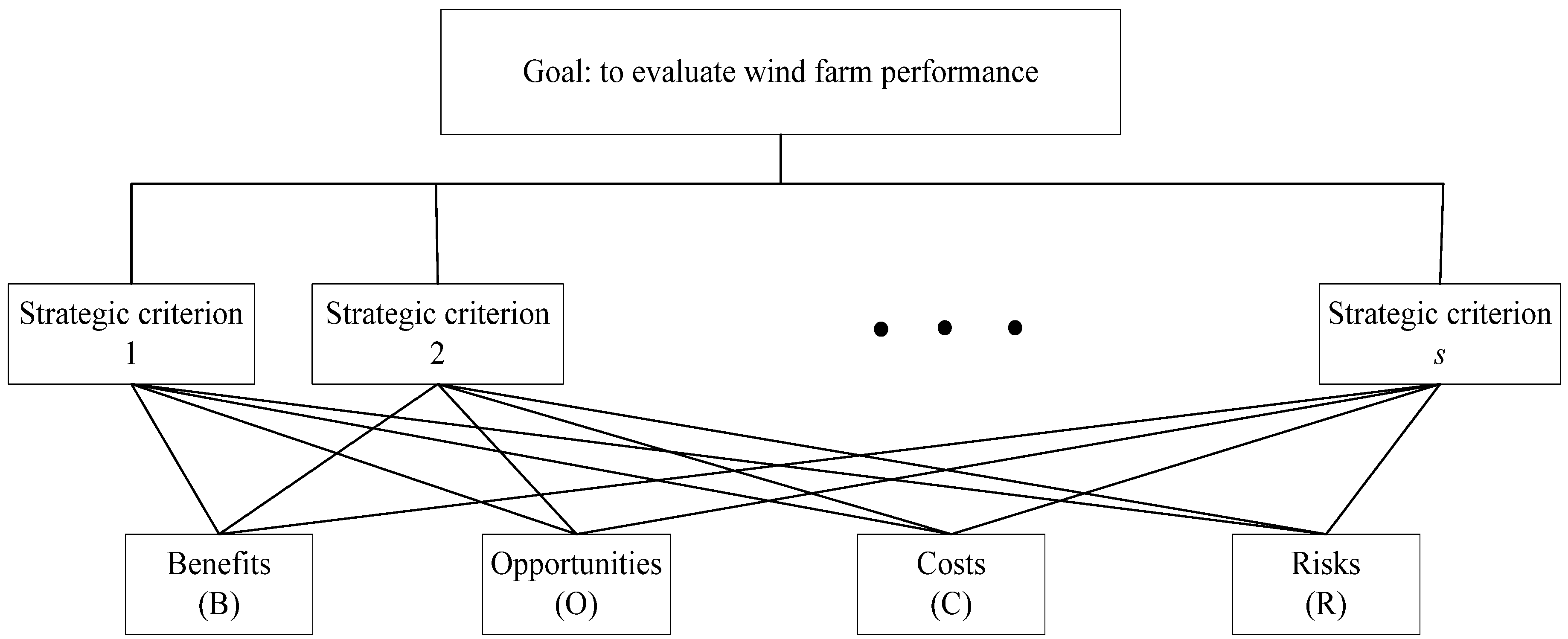
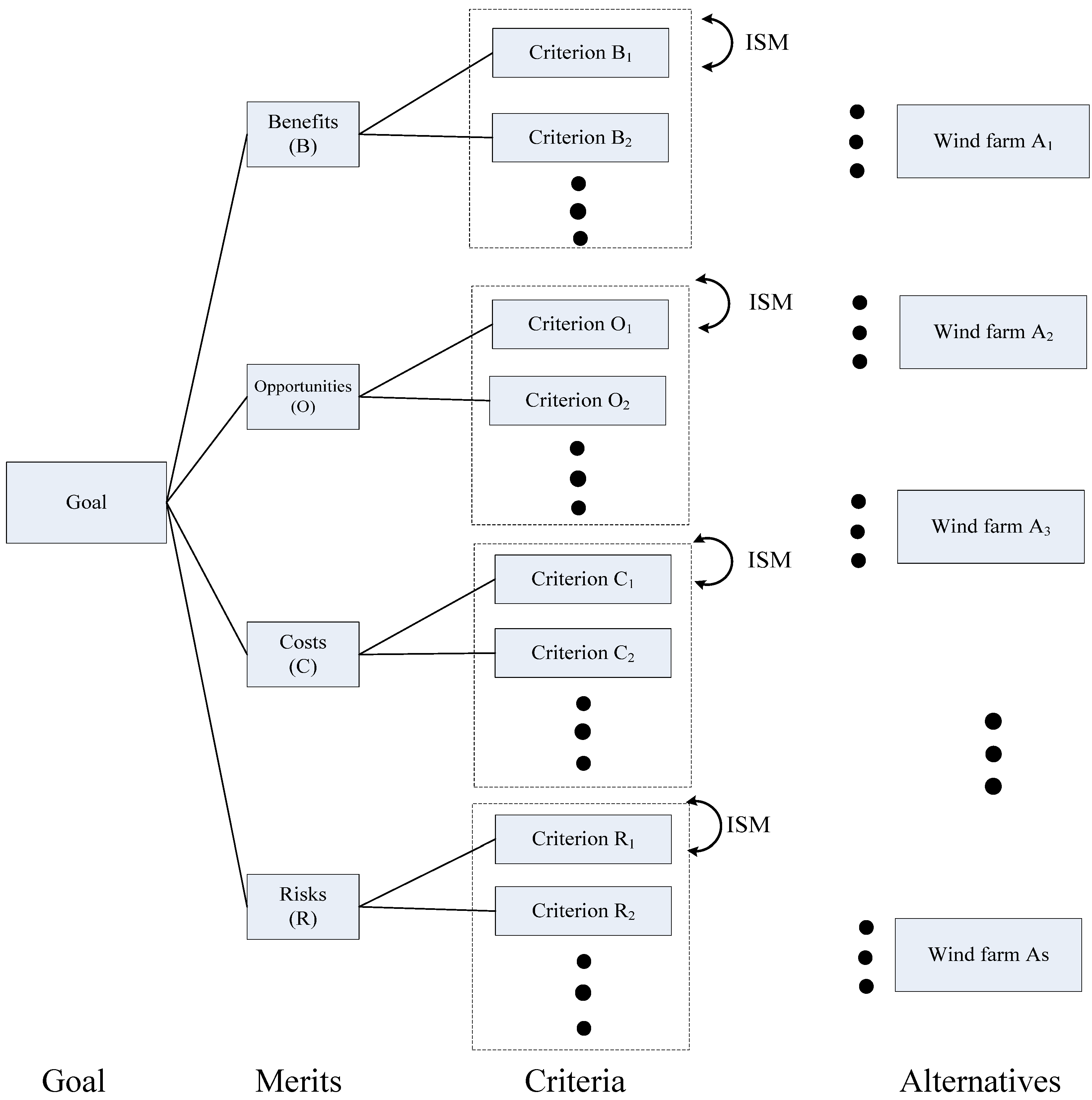
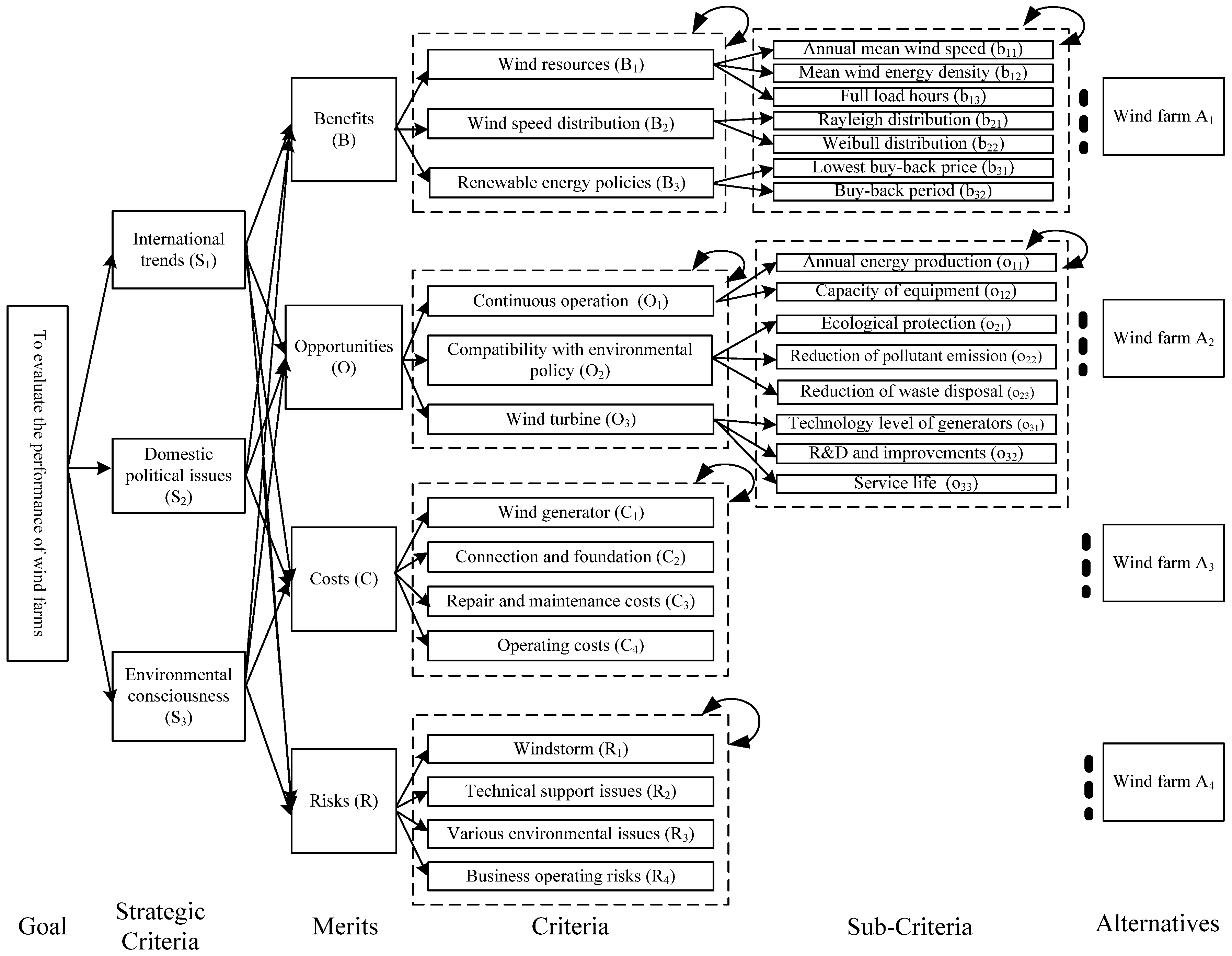
- Step 8. Decompose the wind farm evaluation problem into a network with four sub-networks. With literature review and experts’ opinions, we can construct a network in the form as in Figure 5. Four merits (B, O, C, R) must be considered in achieving the overall goal, and a sub-network is formed for each of the merits. For example, for the benefits (B) sub-network, there are criteria that are related to the achievement of the benefits of the ultimate goal, and the lowest level contains the wind farms that are under evaluation.Figure 5. The BOCR with ISM network.
![Energies 04 02002 g005]()
- Step 9. Construct adjacency matrix (i.e., relation matrix) for the criteria under each merit. For each merit M, establish relation matrix , using the criteria identified in Step 8, to show the contextual relationship among the criteria. Experts, through a questionnaire or the Delphi method, are invited to identify the contextual relationship between any two criteria, and the associated direction of the relation. The relation matrix is presented as follows:where denotes the relation between criteria and , and =1 if xj is reachable from xi,; otherwise, =0.
- Step 10. Develop initial reachability matrix for each merit and check for transitivity. The initial reachability matrix is calculated by adding with the unit matrix I:
- Step 11. Develop final reachability matrix for each merit. The transitivity of the contextual relation means that if criterion xi is related to xj and xj is related to xp, then xi is necessarily related to xp. Under the operators of the Boolean multiplication and addition (i.e., 0 × 0 = 0, 1 × 0 = 0 × 1 = 0, 1 × 1 = 1, 0 + 0 = 0, 1 + 0 = 0 + 1 = 1, 1 + 1 = 1), a convergence can be met:where denotes the impact of criterion xi to criterion xj under merit M.
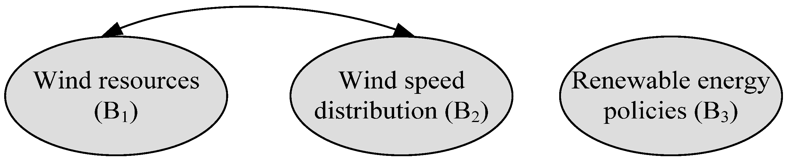
- Step 12. Construct a sub-network for each merit based on the final reachability matrix for the merit.
- Step 13. Employ a questionnaire to collect experts’ opinions on the BOCR with ISM network. Formulate a questionnaire based on the network in Figure 5 and the sub-networks constructed in Step 12 to pairwise compare the importance of the criteria under each merit, and the interdependence among the criteria under each merit. The expected relative performance of the alternatives under each criterion is determined by the experts using seven different linguistic terms, as depicted in Figure 3.
- Step 14. Calculate the relative priorities under each merit sub-network. A similar procedure as in Steps 4 and 5 is applied to establish relative importance weights of the criteria with respect to the same upper-level merit, the interdependence of the criteria with respect to the same upper-level merit, and the expected relative performance of alternatives with respect to each criterion.
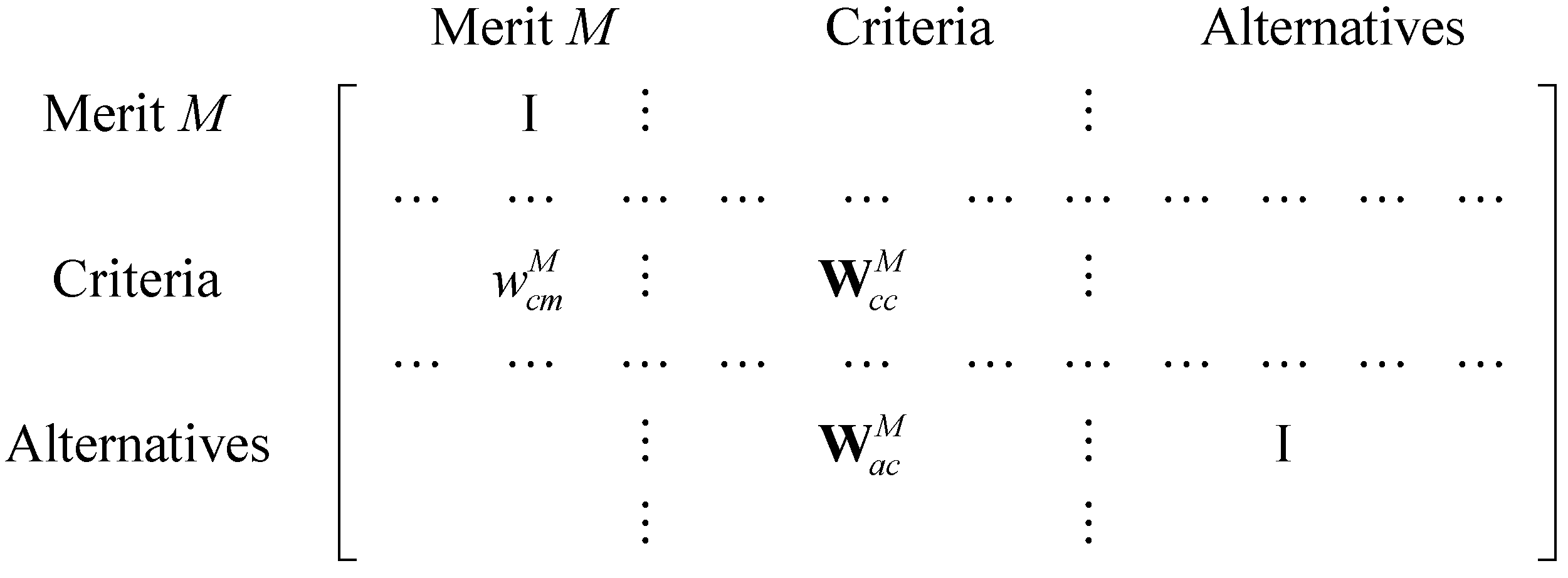
- Step 15. Calculate the priorities of alternatives for each merit sub-network. Using the priorities obtained from Step 14, form an unweighted supermatrix for merit M, as depicted in Figure 6, where is a vector that represents the impact of merit M on the criteria, indicates the interdependency of the criteria, is a matrix that represents the impact of criteria on each of the alternatives, and is the identity matrix. A weighted supermatrix and a limit supermatrix for each sub-network can be calculated by ANP, which is proposed by Saaty [32]. The priorities of the alternatives under each merit are calculated by normalizing the alternative-to-goal column of the limit supermatrix of the merit.
- Step 16. Calculate overall priorities of the alternatives by synthesizing priorities of each alternative under each merit from Step 15 with corresponding normalized weights b, o, c and r from Step 7. There are five ways to calculate the overall priority of each alternative under B, O, C and R, as shown in Equations (4) to (8) [34].


4. Case Study
| Merits | Criteria/Sub-criteria | Definition |
|---|---|---|
| Benefits | (B1) Wind resources | Estimation of energy production of a wind farm. |
| (b11) Annual mean wind speed | Annual average (mean) wind speed for a given location (meters per second, m/s) | |
| (b12) Mean wind energy density | Wind power density, measured in watts per square meter, indicating how much energy is available at the site for conversion by a wind turbine. | |
| (b13) Full load hours | Average hours of full load of a wind turbine per year. | |
| (B2) Wind speed distribution | Estimation of the distribution of wind speeds throughout the year | |
| (b21) Rayleigh distribution | The Rayleigh distribution may be used as a model for wind speed. It can estimate the energy recovered by a wind turbine. | |
| (b22) Weibull distribution | The Weibull distribution may be used to describe the variations in wind speeds. | |
| (B3) Renewable energy policies | The utility company and the wind farm have an agreement on the buy back of electricity supplied by a wind farm. | |
| (b31) Lowest buy-back price | The utility company offers a lowest buy-back price to buy back electricity. | |
| (b32) Buy-back period | The utility company offers to buy back electricity in a specified duration of time. | |
| Opportunities | (O1) Continuous operation | The continuous and reliable operation of the wind farm. |
| (o11) Annual energy production | Expected annual energy generated from the wind farm. | |
| (o12) Capacity of equipment | Expected capacity of equipment after deducting downtime and maintenance time. | |
| (O2) Compatibility with environmental policy | The degree of convergence between the environmental policy and the operation of the wind farm. | |
| (o21) Ecological protection | The ecological benefits obtained from the wind farm in generating energy compared to traditional energy sources. | |
| (o22) Reduction of pollutant emission | The reduction of pollutant emission, such as CO2 and SO2, from the wind farm in generating energy compared to traditional energy sources. | |
| (o23) Reduction of waste disposal | The reduction of waste, which can damage the environment from the wind farm in generating energy, compared to traditional energy sources. | |
| (O3) Wind turbine | The expected operation of wind turbines. | |
| (o31) Technology level of generators | Technology that can be obtained from operating generators. | |
| (o32) R&D and improvements | R&D level and improvements that can be achieved in the equipment other than generators. | |
| (o33) Service life | Expected useful life of wind turbines. | |
| Costs | (C1) Wind generator | The cost of wind generators. |
| (C2) Connection and foundation | The cost of connection and foundations in constructing wind turbines. | |
| (C3) Repair and maintenance costs | Repair and maintenance costs incurred in operating the wind farm. | |
| (C4) Operating costs | Operating costs of the wind farm in generating energy. | |
| Risks | (R1) Windstorm | The severity of windstorms may disable the operation of the wind farm. |
| (R2) Technical support issues | Local technical problems may arise because some equipment is purchased overseas. | |
| (R3) Various environmental issues | The negative impacts of the wind farm to the environment, such as bird deaths, aesthetics and noise. | |
| (R4) Business operating risks | Risks arising from the execution of the wind farm’s business functions, and including the risks arising from the people, systems, processes and financial conditions. |
| S1 | S2 | S3 | |
|---|---|---|---|
| Benefits | (0.715, 0.828, 0.865, 0.883) | (0.682, 0.761, 0.832, 0.866) | (0.546, 0.683, 0.714, 0.782) |
| Opportunities | (0.292, 0.398, 0.398, 0.531) | (0.464, 0.590, 0.590, 0.696) | (0.507, 0.597, 0.624, 0.726) |
| Costs | (0.178, 0.247, 0.323, 0.394) | (0.247, 0.323, 0.370, 0.472) | (0.368, 0.485, 0.485, 0.608) |
| Risks | (0.114, 0.126, 0.144, 0.280) | (0.208, 0.262, 0.343, 0.419) | (0.178, 0.247, 0.323, 0.394) |
| S1 (0.521) | S2 (0.278) | S3 (0.201) | Overall priorities | Normalized priorities | |
|---|---|---|---|---|---|
| Benefits | 0.823 | 0.785 | 0.681 | 0.784 | 0.423 |
| Opportunities | 0.405 | 0.585 | 0.613 | 0.497 | 0.268 |
| Costs | 0.285 | 0.353 | 0.487 | 0.345 | 0.186 |
| Risks | 0.166 | 0.308 | 0.285 | 0.229 | 0.124 |


| g | B1 | B2 | B3 | b11 | b12 | b13 | b21 | b22 | b31 | b32 | A1 | A2 | A3 | A4 | |
|---|---|---|---|---|---|---|---|---|---|---|---|---|---|---|---|
| g | 1 | 0 | 0 | 0 | 0 | 0 | 0 | 0 | 0 | 0 | 0 | 0 | 0 | 0 | 0 |
| B1 | 0.27877 | 0.5 | 0.5 | 0 | 0 | 0 | 0 | 0 | 0 | 0 | 0 | 0 | 0 | 0 | 0 |
| B2 | 0.22280 | 0.5 | 05 | 0 | 0 | 0 | 0 | 0 | 0 | 0 | 0 | 0 | 0 | 0 | 0 |
| B3 | 0.49843 | 0 | 0 | 1 | 0 | 0 | 0 | 0 | 0 | 0 | 0 | 0 | 0 | 0 | 0 |
| b11 | 0 | 0.28488 | 0 | 0 | 0.22621 | 0.18215 | 0.19164 | 0.19093 | 0.18169 | 0 | 0 | 0 | 0 | 0 | 0 |
| b12 | 0 | 0.21740 | 0 | 0 | 0.20656 | 0.20430 | 0.19180 | 0.20233 | 0.19414 | 0 | 0 | 0 | 0 | 0 | 0 |
| b13 | 0 | 0.49772 | 0 | 0 | 0.19884 | 0.20703 | 0.19651 | 0.19591 | 0.19073 | 0 | 0 | 0 | 0 | 0 | 0 |
| b21 | 0 | 0 | 0.5 | 0 | 0.18704 | 0.19211 | 0.20832 | 0.21735 | 0.21517 | 0 | 0 | 0 | 0 | 0 | 0 |
| b22 | 0 | 0 | 0.5 | 0 | 0.18136 | 0.21440 | 0.21174 | 0.19347 | 0.21827 | 0 | 0 | 0 | 0 | 0 | 0 |
| b31 | 0 | 0 | 0 | 0.75 | 0 | 0 | 0 | 0 | 0 | 1 | 0 | 0 | 0 | 0 | 0 |
| b32 | 0 | 0 | 0 | 0.25 | 0 | 0 | 0 | 0 | 0 | 0 | 1 | 0 | 0 | 0 | 0 |
| A1 | 0 | 0 | 0 | 0 | 0.34747 | 0.32230 | 0.50355 | 0.22361 | 0.46891 | 0.23058 | 0.25058 | 1 | 0 | 0 | 0 |
| A2 | 0 | 0 | 0 | 0 | 0.13922 | 0.13743 | 0.14563 | 0.23300 | 0.15262 | 0.18832 | 0.24913 | 0 | 1 | 0 | 0 |
| A3 | 0 | 0 | 0 | 0 | 0.33228 | 0.37174 | 0.22574 | 0.20282 | 0.25823 | 0.44495 | 0.20642 | 0 | 0 | 1 | 0 |
| A4 | 0 | 0 | 0 | 0 | 0.18103 | 0.16852 | 0.12508 | 0.34058 | 0.12023 | 0.13615 | 0.23986 | 0 | 0 | 0 | 1 |
| g | B1 | B2 | B3 | b11 | b12 | b13 | b21 | b22 | b31 | b32 | A1 | A2 | A3 | A4 | |
|---|---|---|---|---|---|---|---|---|---|---|---|---|---|---|---|
| g | 0.5 | 0 | 0 | 0 | 0 | 0 | 0 | 0 | 0 | 0 | 0 | 0 | 0 | 0 | 0 |
| B1 | 0.13939 | 0.25 | 0.25 | 0 | 0 | 0 | 0 | 0 | 0 | 0 | 0 | 0 | 0 | 0 | 0 |
| B2 | 0.11140 | 0.25 | 2.5 | 0 | 0 | 0 | 0 | 0 | 0 | 0 | 0 | 0 | 0 | 0 | 0 |
| B3 | 0.24922 | 0 | 0 | 0.5 | 0 | 0 | 0 | 0 | 0 | 0 | 0 | 0 | 0 | 0 | 0 |
| b11 | 0 | 0.14244 | 0 | 0 | 0.11311 | 0.09108 | 0.09582 | 0.09547 | 0.09085 | 0 | 0 | 0 | 0 | 0 | 0 |
| b12 | 0 | 0.10870 | 0 | 0 | 0.10328 | 0.10215 | 0.09590 | 0.10117 | 0.09707 | 0 | 0 | 0 | 0 | 0 | 0 |
| b13 | 0 | 0.24886 | 0 | 0 | 0.09942 | 0.10352 | 0.09826 | 0.09796 | 0.09537 | 0 | 0 | 0 | 0 | 0 | 0 |
| b21 | 0 | 0 | 0.25 | 0 | 0.09352 | 0.09606 | 0.10416 | 0.10868 | 0.10759 | 0 | 0 | 0 | 0 | 0 | 0 |
| b22 | 0 | 0 | 0.25 | 0 | 0.09068 | 0.10720 | 0.10587 | 0.09674 | 0.10914 | 0 | 0 | 0 | 0 | 0 | 0 |
| b31 | 0 | 0 | 0 | 0.375 | 0 | 0 | 0 | 0 | 0 | 0.5 | 0 | 0 | 0 | 0 | 0 |
| b32 | 0 | 0 | 0 | 0.125 | 0 | 0 | 0 | 0 | 0 | 0 | 0.5 | 0 | 0 | 0 | 0 |
| A1 | 0 | 0 | 0 | 0 | 0.17374 | 0.16115 | 0.25178 | 0.11181 | 0.23446 | 0.11529 | 0.12529 | 1 | 0 | 0 | 0 |
| A2 | 0 | 0 | 0 | 0 | 0.06961 | 0.06872 | 0.07282 | 0.11650 | 0.07631 | 0.09416 | 0.12457 | 0 | 1 | 0 | 0 |
| A3 | 0 | 0 | 0 | 0 | 0.16614 | 0.18587 | 0.11287 | 0.10141 | 0.12912 | 0.22248 | 0.10321 | 0 | 0 | 1 | 0 |
| A4 | 0 | 0 | 0 | 0 | 0.09052 | 0.08426 | 0.06254 | 0.17029 | 0.06012 | 0.06807 | 0.11993 | 0 | 0 | 0 | 1 |
| g | B1 | B2 | B3 | b11 | b12 | b13 | b21 | b22 | b31 | b32 | A1 | A2 | A3 | A4 | |
|---|---|---|---|---|---|---|---|---|---|---|---|---|---|---|---|
| g | 0 | 0 | 0 | 0 | 0 | 0 | 0 | 0 | 0 | 0 | 0 | 0 | 0 | 0 | 0 |
| B1 | 0 | 0 | 0 | 0 | 0 | 0 | 0 | 0 | 0 | 0 | 0 | 0 | 0 | 0 | 0 |
| B2 | 0 | 0 | 0 | 0 | 0 | 0 | 0 | 0 | 0 | 0 | 0 | 0 | 0 | 0 | 0 |
| B3 | 0 | 0 | 0 | 0 | 0 | 0 | 0 | 0 | 0 | 0 | 0 | 0 | 0 | 0 | 0 |
| b11 | 0 | 0 | 0 | 0 | 0 | 0 | 0 | 0 | 0 | 0 | 0 | 0 | 0 | 0 | 0 |
| b12 | 0 | 0 | 0 | 0 | 0 | 0 | 0 | 0 | 0 | 0 | 0 | 0 | 0 | 0 | 0 |
| b13 | 0 | 0 | 0 | 0 | 0 | 0 | 0 | 0 | 0 | 0 | 0 | 0 | 0 | 0 | 0 |
| b21 | 0 | 0 | 0 | 0 | 0 | 0 | 0 | 0 | 0 | 0 | 0 | 0 | 0 | 0 | 0 |
| b22 | 0 | 0 | 0 | 0 | 0 | 0 | 0 | 0 | 0 | 0 | 0 | 0 | 0 | 0 | 0 |
| b31 | 0 | 0 | 0 | 0 | 0 | 0 | 0 | 0 | 0 | 0 | 0 | 0 | 0 | 0 | 0 |
| b32 | 0 | 0 | 0 | 0 | 0 | 0 | 0 | 0 | 0 | 0 | 0 | 0 | 0 | 0 | 0 |
| A1 | 0.30741 | 0.38711 | 0.36839 | 0.23558 | 0.35998 | 0.34858 | 0.43827 | 0.29738 | 0.42069 | 0.23058 | 0.25058 | 1 | 0 | 0 | 0 |
| A2 | 0.18374 | 0.15834 | 0.17125 | 0.20352 | 0.15013 | 0.14949 | 0.15395 | 0.19777 | 0.15762 | 0.18832 | 0.24913 | 0 | 1 | 0 | 0 |
| A3 | 0.32702 | 0.27555 | 0.26099 | 0.38532 | 0.30595 | 0.32464 | 0.25132 | 0.24003 | 0.2674 | 0.44495 | 0.20642 | 0 | 0 | 1 | 0 |
| A4 | 0.18183 | 0.17900 | 0.19937 | 0.17558 | 0.18394 | 0.1773 | 0.15646 | 0.26481 | 0.15429 | 0.13615 | 0.29386 | 0 | 0 | 0 | 1 |
| Merits | Benefits | Opportunities | Costs | Risks | ||||
|---|---|---|---|---|---|---|---|---|
| Priorities | 0.423 | 0.268 | 0.186 | 0.124 | ||||
| Alternatives | Normalized | Normalized | Normalized | Reciprocal | Normalized | Normalized | Reciprocal | Normalized |
| Reciprocal | Reciprocal | |||||||
| A1 | 0.30741 | 0.35528 | 0.30827 | 3.24391 | 0.19629 | 0.23282 | 4.29516 | 0.26763 |
| A2 | 0.18374 | 0.18714 | 0.27960 | 3.57654 | 0.21641 | 0.26970 | 3.70782 | 0.23103 |
| A3 | 0.32702 | 0.31219 | 0.20514 | 4.87472 | 0.29497 | 0.24228 | 4.12746 | 0.25718 |
| A4 | 0.18183 | 0.14540 | 0.20699 | 4.83115 | 0.29233 | 0.25520 | 3.91850 | 0.24416 |
| Methods | Additive | Probabilistic additive | Subtractive | Multiplicative priority powers | Multiplicative | |||||
|---|---|---|---|---|---|---|---|---|---|---|
| Alternatives | Priorities | Ranking | Priorities | Ranking | Priorities | Ranking | Priorities | Ranking | Priorities | Ranking |
| A1 | 0.29494 | 2 | 0.44904 | 2 | 0.13904 | 2 | 0.28863 | 2 | 1.52171 | 2 |
| A2 | 0.19678 | 4 | 0.35243 | 4 | 0.04243 | 4 | 0.19550 | 3 | 0.45598 | 4 |
| A3 | 0.30875 | 1 | 0.46380 | 1 | 0.15380 | 1 | 0.30720 | 1 | 2.05410 | 1 |
| A4 | 0.20053 | 3 | 0.35574 | 3 | 0.04574 | 3 | 0.19370 | 4 | 0.50049 | 3 |

| Merits | Criteria/Sub-criteria | Criterion priorities | Sub-criterion priorities | Integrated priorities under the merit | Integrated priorities in the network | Integrated ranking |
|---|---|---|---|---|---|---|
| Benefits (0.423) | (B1) Wind resources | 0.27877 | ||||
| (b11) Annual mean wind speed | 0.28488 | 0.07942 | 0.03359 | 15 | ||
| (b12) Mean wind energy density | 0.21740 | 0.06060 | 0.02563 | 20 | ||
| (b13) Full load hours | 0.49772 | 0.13875 | 0.05869 | 4 | ||
| (B2) Wind speed distribution | 0.22280 | |||||
| (b21) Rayleigh distribution | 0.5 | 0.11140 | 0.04712 | 7 | ||
| (b22) Weibull distribution | 0.5 | 0.11140 | 0.04712 | 7 | ||
| (B3) Renewable energy policies | 0.49843 | |||||
| (b31) Lowest buy-back price | 0.75 | 0.37382 | 0.15813 | 1 | ||
| (b32) Buy-back period | 0.25 | 0.12461 | 0.05271 | 5 | ||
| Opportunities (0.268) | (O1) Continuous operation | 0.19855 | ||||
| (o11) Annual energy production | 0.5 | 0.09928 | 0.02661 | 18 | ||
| (o12) Capacity of equipment | 0.5 | 0.09928 | 0.02661 | 18 | ||
| (O2) Compatibility with environmental policy | 0.45456 | |||||
| (o21) Ecological protection | 0.42634 | 0.19380 | 0.05194 | 6 | ||
| (o22) Reduction of pollutant emission | 0.32536 | 0.14790 | 0.03964 | 12 | ||
| (o23) Reduction of waste disposal | 0.24830 | 0.11287 | 0.03025 | 16 | ||
| (O3) Wind turbine | 0.34689 | |||||
| (o31) Technology level of generators | 0.46316 | 0.16067 | 0.04306 | 10 | ||
| (o32) R&D and improvements | 0.29177 | 0.10121 | 0.02712 | 17 | ||
| (o33) Service life | 0.24507 | 0.08501 | 0.02278 | 21 | ||
| Costs (0.186) | (C1) Wind generator | 0.34982 | 0.34982 | 0.06507 | 2 | |
| (C2) Connection and foundation | 0.31905 | 0.31905 | 0.05934 | 3 | ||
| (C3) Repair and maintenance costs | 0.21789 | 0.21789 | 0.04053 | 11 | ||
| (C4) Operating costs | 0.11325 | 0.11325 | 0.02106 | 22 | ||
| Risks (0.124) | (R1) Windstorm | 0.35521 | 0.35521 | 0.04405 | 9 | |
| (R2) Technical support issues | 0.27870 | 0.27870 | 0.03456 | 14 | ||
| (R3) Various environmental issues | 0.29620 | 0.29620 | 0.03673 | 13 | ||
| (R4) Business operating risks | 0.06988 | 0.06988 | 0.00867 | 23 |
| Criteria/Sub-criteria | A1 | A2 | A3 | A4 |
|---|---|---|---|---|
| (B1) Wind resources | 0.38711 | 0.15834 | 0.27555 | 0.17900 |
| (b11) Annual mean wind speed | 0.35998 | 0.15013 | 0.30595 | 0.18394 |
| (b12) Mean wind energy density | 0.34858 | 0.14949 | 0.32464 | 0.1773 |
| (b13) Full load hours | 0.43827 | 0.15395 | 0.25132 | 0.15646 |
| (B2) Wind speed distribution | 0.36839 | 0.17125 | 0.26099 | 0.19937 |
| (b21) Rayleigh distribution | 0.29738 | 0.19777 | 0.24003 | 0.26481 |
| (b22) Weibull distribution | 0.42069 | 0.15762 | 0.2674 | 0.15429 |
| (B3) Renewable energy policies | 0.23558 | 0.20352 | 0.38532 | 0.17558 |
| (b31) Lowest buy-back price | 0.23058 | 0.18832 | 0.44495 | 0.13615 |
| (b32) Buy-back period | 0.25058 | 0.24913 | 0.20642 | 0.29386 |
| (O1) Continuous operation | 0.34600 | 0.17919 | 0.32437 | 0.15044 |
| (o11) Annual energy production | 0.35839 | 0.17069 | 0.31497 | 0.15595 |
| (o12) Capacity of equipment | 0.33366 | 0.18756 | 0.33857 | 0.14021 |
| (O2) Compatibility with environmental policy | 0.36703 | 0.19597 | 0.30328 | 0.13372 |
| (o21) Ecological protection | 0.39645 | 0.17855 | 0.29645 | 0.12855 |
| (o22) Reduction of pollutant emission | 0.35099 | 0.22272 | 0.29646 | 0.12983 |
| (o23) Reduction of waste disposal | 0.33752 | 0.19084 | 0.32393 | 0.14772 |
| (O3) Wind turbine | 0.34595 | 0.17930 | 0.31958 | 0.15517 |
| (o31) Technology level of generators | 0.37304 | 0.15305 | 0.32974 | 0.14417 |
| (o32) R&D and improvements | 0.35755 | 0.16966 | 0.31569 | 0.15711 |
| (o33) Service life | 0.28075 | 0.24087 | 0.28543 | 0.19295 |
| (C1) Wind generator | 0.34959 | 0.35074 | 0.16062 | 0.13904 |
| (C2) Connection and foundation | 0.27363 | 0.23576 | 0.21463 | 0.27598 |
| (C3) Repair and maintenance costs | 0.31317 | 0.25176 | 0.25198 | 0.18310 |
| (C4) Operating costs | 0.26878 | 0.23694 | 0.22580 | 0.26849 |
| (R1) Windstorm | 0.23451 | 0.26127 | 0.23302 | 0.27120 |
| (R2) Technical support issues | 0.22807 | 0.25092 | 0.24515 | 0.27587 |
| (R3) Various environmental issues | 0.24346 | 0.26973 | 0.26681 | 0.22000 |
| (R4) Business operating risks | 0.19806 | 0.38736 | 0.17392 | 0.24067 |
5. Conclusions
Acknowledgement
References
- Lenzen, M. Current state of development of electricity-generating technologies: A literature review. Energies 2010, 3, 462–591. [Google Scholar] [CrossRef]
- Takuno, T.; Kitamori, Y.; Takahashi, R.; Hikihara, T. AC power routing system in home based on demand and supply utilizing distributed power sources. Energies 2011, 4, 717–726. [Google Scholar] [CrossRef] [Green Version]
- Deng, Y.; Yu, Z.; Liu, S. A review on scale and siting of wind farms in China. Wind Energy 2011, 14, 463–470. [Google Scholar] [CrossRef]
- Probst, O.; Cárdenas, D. State of the art and trends in wind resource assessment. Energies 2010, 3, 1087–1141. [Google Scholar] [CrossRef]
- Kahraman, C.; Kaya, I.; Cebi, S. A comparative analysis for multiattribute selection among renewable energy alternatives using fuzzy axiomatic design and fuzzy analytic hierarchy process. Energy 2009, 34, 1603–1616. [Google Scholar] [CrossRef]
- San Cristóbal, J.R. Multi-criteria decision-making in the selection of a renewable energy project in Spain: The Vikor method. Renew. Energy 2011, 36, 498–502. [Google Scholar] [CrossRef]
- Kaya, T.; Kahraman, C. Multicriteria renewable energy planning using an integrated fuzzy VIKOR & AHP methodology: The case of Istanbul. Energy 2010, 35, 2517–2527. [Google Scholar] [CrossRef]
- Warfield, J.N. Developing interconnected matrices in structural modeling. IEEE Trans. Syst. Man Cybern. 1974, 4, 51–81. [Google Scholar]
- Warfield, J.N. Toward interpretation of complex structural modeling. IEEE Trans. Syst. Man Cybern. 1974, 4, 405–417. [Google Scholar] [CrossRef]
- Warfield, J.N. Societal Systems: Planning, Policy and Complexity; John Wiley & Sons: New York, NY, USA, 1976. [Google Scholar]
- Huang, J.J.; Tzeng, G.H.; Ong, C.S. Multidimensional data in multidimensional scaling using the analytic network process. Pat. Recogn. Lett. 2005, 26, 755–767. [Google Scholar] [CrossRef]
- Sahney, S.; Banwet, D.K.; Karunes, S. An integrated framework for quality in education: Application of quality function deployment, interpretive structural modelling and path analysis. Total Qual. Manag. Bus. 2006, 17, 265–285. [Google Scholar] [CrossRef]
- Agarwal, R.S.; Tiwari, M.K. Modeling agility of supply chain. Ind. Market. Manag. 2007, 36, 443–457. [Google Scholar] [CrossRef]
- Thakkar, J.; Deshmukh, S.G.; Gupta, A.D.; Shankar, R. Development of a balanced scorecard: An integrated approach of interpretive structural modeling (ISM) and analytic network process (ANP). Int. J. Product. Perf. Manag. 2007, 56, 25–59. [Google Scholar] [CrossRef]
- Faisal, M.N.; Banwet, D.K.; Shankar, R. Information risks management in supply chains: An assessment and mitigation framework. J. Ent. Inform. Manag. 2007, 20, 677–699. [Google Scholar] [CrossRef]
- Kannan, G.; Haq, A.N. Analysis of interactions of criteria and sub-criteria for the selection of supplier in the built-in-order supply chain environment. Int. J. Prod. Res. 2007, 45, 831–852. [Google Scholar] [CrossRef]
- Qureshi, M.N.; Kumar, D.; Kumar, P. Modeling the logistics outsourcing relationship variables to enhance shippers’ productivity and competitiveness in logistical supply chain. Int. J. Product. Perf. Manag. 2007, 56, 689–714. [Google Scholar] [CrossRef]
- Singh, R.K.; Garg, S.K.; Deshmukh, S.G.; Kumar, M. Modelling of critical success factors for implementation of AMTs. J. Model. Manag. 2007, 2, 232–250. [Google Scholar] [CrossRef]
- Upadhyay, R.K.; Gaur, S.K.; Agrawal, V.P.; Arora, K.C. ISM-CMAP-Combine (ICMC) for hierarchical knowledge scenario in quality engineering education. Eur. J. Eng. Educ. 2007, 32, 21–33. [Google Scholar] [CrossRef]
- Thakkar, J.; Kanda, A.; Deshmukh, S.G. Evaluation of buyer-supplier relationships using an integrated mathematical approach of interpretive structural modeling (ISM) and graph theoretic matrix. J. Manuf. Technol. Manag. 2008, 19, 92–124. [Google Scholar] [CrossRef]
- Vivek, S.D.; Banwet, D.K.; Shankar, R. Analysis of interactions among core, transaction and relationship-specific investments: The case of offshoring. J. Oper. Manag. 2008, 26, 180–197. [Google Scholar] [CrossRef]
- Yang, J.J.; Tzeng, H.N.; Yeh, R.H. Vendor selection by integrated fuzzy MCDM techniques with independence and interdependence. Inf. Sci. 2008, 178, 4166–4183. [Google Scholar] [CrossRef]
- Wang, G.H.; Wang, Y.X.; Zhao, T. Analysis of interactions among the barriers to energy saving in China. Energy Policy 2008, 36, 1879–1889. [Google Scholar] [CrossRef]
- Chidambaranathan, S.; Muralidharan, C.; Deshmukh, S.G. Analyzing the interaction of critical factors of supplier development using Interpretive Structural Modeling—an empirical study. Int. J. Adv. Manuf. Technol. 2009, 43, 1081–1093. [Google Scholar] [CrossRef]
- Kannan, G.; Pokharel, S.; Kumar, P.S. A hybrid approach using ISM and fuzzy TOPSIS for the selection of reverse logistics provider. Resour. Conserv. Recycl. 2009, 54, 28–36. [Google Scholar] [CrossRef]
- Mukherjee, K.; Mondal, S. Analysis of issues relating to remanufacturing technology of an Indian company—a case of an Indian company. Technol. Anal. Strategy. Manag. 2009, 21, 639–652. [Google Scholar] [CrossRef]
- Feng, C.M.; Wu, P.J.; Chia, K.C. A hybrid fuzzy integral decision-making model for locating manufacturing centers in China: A case study. Eur. J. Oper. Res. 2010, 200, 63–73. [Google Scholar] [CrossRef]
- Lee, A.H.I.; Wang, W.M.; Lin, T.Y. An evaluation framework for technology transfer of new equipment in high technology industry. Technol. Forecast. Soc. 2010, 77, 135–150. [Google Scholar] [CrossRef]
- Lee, A.H.I.; Chen, H.H.; Kang, H.Y. A model to analyze strategic products for photovoltaic silicon thin-film solar cell power industry. Renew. Sust. Energ. Rev. 2011, 15, 1271–1283. [Google Scholar] [CrossRef]
- Lee, A.H.I.; Kang, H.Y.; Chang, C.C. An integrated interpretive structural modeling-fuzzy analytic network process-benefits, opportunities, costs and risks model for selecting technologies. Int. J. Inf. Technol. Decis. Mak. 2011, 10, 843–871. [Google Scholar] [CrossRef]
- Saaty, T.L. The Analytic Hierarchy Process; McGraw-Hill: New York, NY, USA, 1980. [Google Scholar]
- Saaty, T.L. Decision Making with Dependence and Feedback: The Analytic Network Process; RWS Publications: Pittsburgh, PA, USA, 1996. [Google Scholar]
- Meade, L.M.; Sarkis, J. Analyzing organizational project alternatives for agile manufacturing processes: An analytical network approach. Int. J. Prod. Res. 1999, 37, 241–261. [Google Scholar] [CrossRef]
- Saaty, R.W. Decision Making in Complex Environment: The Analytic Hierarchy Process (AHP) for Decision Making and the Analytic Network Process (ANP) for Decision Making with Dependence and Feedback; Super Decisions: Pittsburgh, PA, USA, 2003. [Google Scholar]
- Lee, A.H.I. A fuzzy AHP evaluation model for buyer-supplier relationships with the consideration of benefits, opportunities, costs and risks. Int. J. Prod. Res. 2009, 47, 4255–4280. [Google Scholar] [CrossRef]
- Yager, R.R. A procedure for ordering fuzzy subsets of the unit interval. Inf. Sci. 1981, 24, 143–161. [Google Scholar] [CrossRef]
© 2011 by the authors; licensee MDPI, Basel, Switzerland. This article is an open access article distributed under the terms and conditions of the Creative Commons Attribution license (http://creativecommons.org/licenses/by/3.0/).
Share and Cite
Kang, H.-Y.; Hung, M.-C.; Pearn, W.L.; Lee, A.H.I.; Kang, M.-S. An Integrated Multi-Criteria Decision Making Model for Evaluating Wind Farm Performance. Energies 2011, 4, 2002-2026. https://doi.org/10.3390/en4112002
Kang H-Y, Hung M-C, Pearn WL, Lee AHI, Kang M-S. An Integrated Multi-Criteria Decision Making Model for Evaluating Wind Farm Performance. Energies. 2011; 4(11):2002-2026. https://doi.org/10.3390/en4112002
Chicago/Turabian StyleKang, He-Yau, Meng-Chan Hung, W. L. Pearn, Amy H. I. Lee, and Mei-Sung Kang. 2011. "An Integrated Multi-Criteria Decision Making Model for Evaluating Wind Farm Performance" Energies 4, no. 11: 2002-2026. https://doi.org/10.3390/en4112002