A Transient Model for Fuel Cell Cathode-Water Propagation Behavior inside a Cathode after a Step Potential


Abstract
:1. Introduction
2. Proposed Model
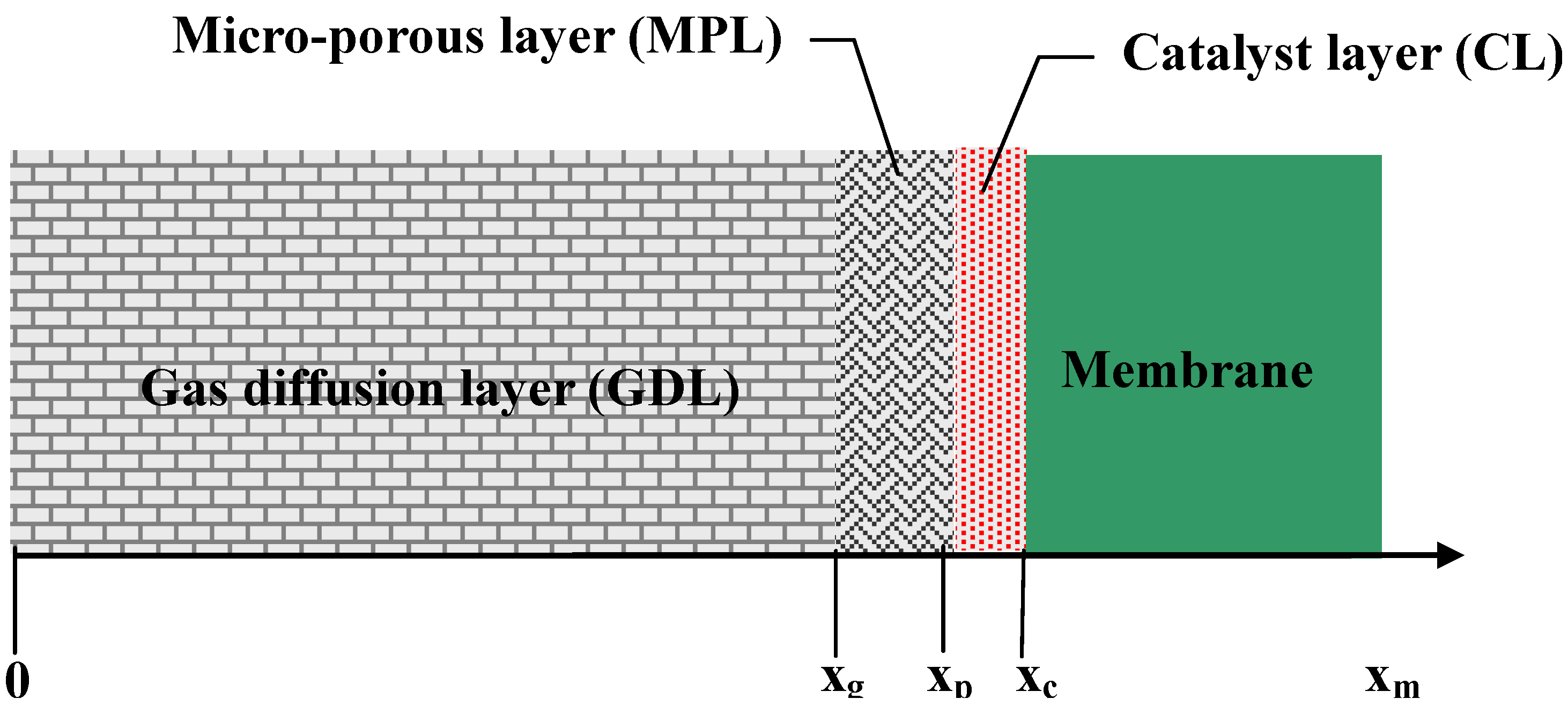
2.1. Physical Model
- (1)
- This is a one-dimensional model. It only considers the variation across the electrode.
- (2)
- The temperature across the electrode is assumed to be constant.
- (3)
- The properties of a given layer are assumed to be constant throughout the entire layer. These properties include contact angle, porosity, ionic conductivity in the liquid phase, electrical conductivity in the solid phase, exchange current density, and charge transfer coefficient in the CL, etc.
- (4)
- The oxygen outside the electrode is assumed to be uniform and its molar fraction is 0.21.
- (5)
- The water saturation is constant at 1.0 in the membrane.

2.2. Gas Diffusion Layer (GDL)


2.3. Micro-Porous Layer (MPL)
2.4. Catalyst Layer (CL)
- (1)
- The water flow due to capillary force (u2 ∂ S/∂ x),
- (2)
- The evaporation/condensation of water (K2,C S [Y2sat – Y2 ]),
- (3)
- Migration of water due to electro-osmosis drag (λ ii ∂S/∂ x) m2/(2F ρ2)), and
- (4)
- Water generated due to electrochemical reaction (ie m2/(2F ρ2)).

3. Numerical Method

| Parameter | Value | |
|---|---|---|
| Temperature | T | 338 K |
| Pressure of gas phase | P | 1.013 × 10⁶ g cm-1 s-2 |
| Active surface area per unit volume of porous electrode | a | 2.2 × 105 cm-1 |
| Tafel slope of ORR | b | 0.06 V decade-1 |
| Oxygen diffusion coefficient in gas phase | D1,g | 0.18 cm2 s-1 |
| Water vapor in gas phase | D2,g | 0.2 cm2 s-1 |
| Open cell voltage | EOCV | 1.15 V |
| Exchange current density of oxygen reduction reaction | i0 | 1.0 × 10⁻⁷A cm-2 |
| Pressure of gas phase | Pg | 1.013 × 10⁶ g cm-1 s-2 |
| Saturation at x = 0 | Sx = 0 | 0.1 |
| Saturation at x = xc | Sx = xc | 1.0 |
| Distance measured from the cathode surface to the interface between CL and membrane | xC | 0.038 cm |
| Distance measured from the cathode surface to the interface between GDL and MPL | xG | 0.03 cm |
| Distance measured from the cathode surface to the interface between MPL and CL of cathode | xP | 0.035 cm |
| Molar fraction of oxygen in gas phase at cathode surface | Y1,x = 0 | 0.21 |
| Molar fraction of water vapor in gas phase at interface | 0.1 | |
| Molar fraction of water vapor in gas phase at cathode surface | Y2,x = 0 | 0.01 |
| Electro-osmosis drag, moles of water per mole of H+ | λ | 2.5 |
| Contact angle of carbon | θcc | 45o |
| Electro-osmosis drag, moles of water per mole of H+ | λ | 2.5 |
- (1)
- Initial saturation, S, defining saturation region was given by initial and boundary conditions, S = 0.1 at x = 0 and S = 1.0 at x = 1.0. This value was used to calculate water velocity u2.
- (2)
- Used finite volume method to compute Y1, Y2, φe, and φi by the initial and boundary conditions as well as the initial value of saturation.
- (3)
- Finally, the saturation was updated to give a new distribution of saturation by new values of u2, ii, Y2, and ie. The above three steps were repeated to advance the solution to the next time interval.
| Parameter | value | |
|---|---|---|
| GDL properties | ||
| Electrical conductivity in solid phase | KeG | 1.82 S cm-1 |
| Permeability | Kp,G | 1.0 × 10⁻¹⁰ cm2 |
| Evaporation coefficient of water in gas phase | K2,G | 5 × 10⁻³ mol cm-3 s-1 |
| Porosity | εG | 0.75 |
| Contact angle | θTG | 120 o |
| Tortuosity | τG | 2.75 |
| MPL properties | ||
| Electrical conductivity in solid phase | KeP | 1.98 S cm-1 |
| Permeability | Kp,P | 1.0 × 10⁻¹¹ cm2 |
| Evaporation coefficient of water in gas phase | K2,P | 5 × 10⁻³ mol cm-3 s-1 |
| Porosity | εP | 0.6 |
| Contact angle | θTp | 140 o |
| Tortuosity | τP | 3.0 |
| CL properties | ||
| Electrical conductivity in solid phase | KeC | 1.98 S cm-1 |
| Permeability | Kp,C | 1.0 × 10⁻¹² cm2 |
| Evaporation coefficient of water in gas phase | K2,C | 5 × 10⁻³ mol cm-3 s-1 |
| Ionic conductivity in liquid phase | Ki,C | 0.06 S cm-1 |
| Porosity | εC | 0.5 |
| Contact angle | θTC | 135 o |
| Tortuosity | τC | 3.0 |
| Membrane properties | ||
| Permeability | Kp,M | 1.0 × 10⁻¹³ cm2 |
| Wetting contact angle | θwM | 80 o |
| Porosity | εM | 0.5 |
| Tortuosity | τP | 3.0 |
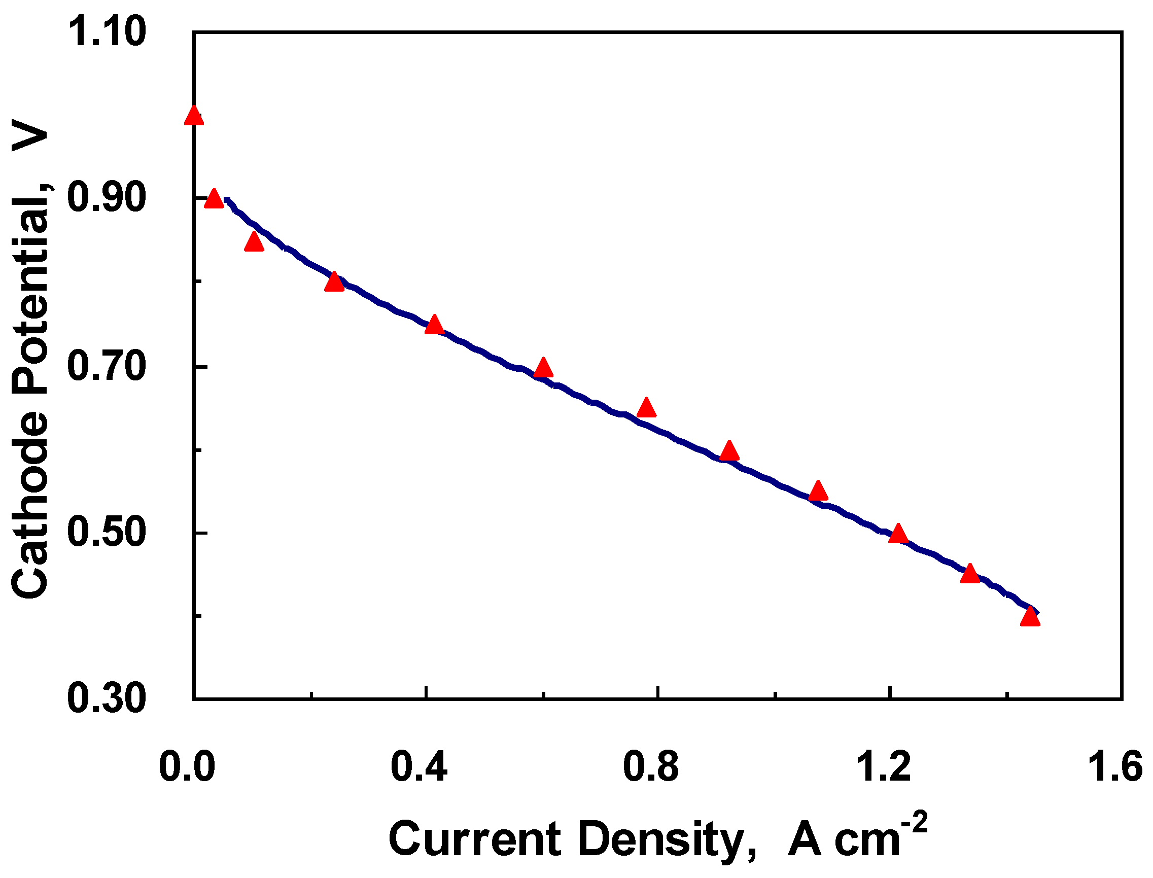
4. Results and Discussion
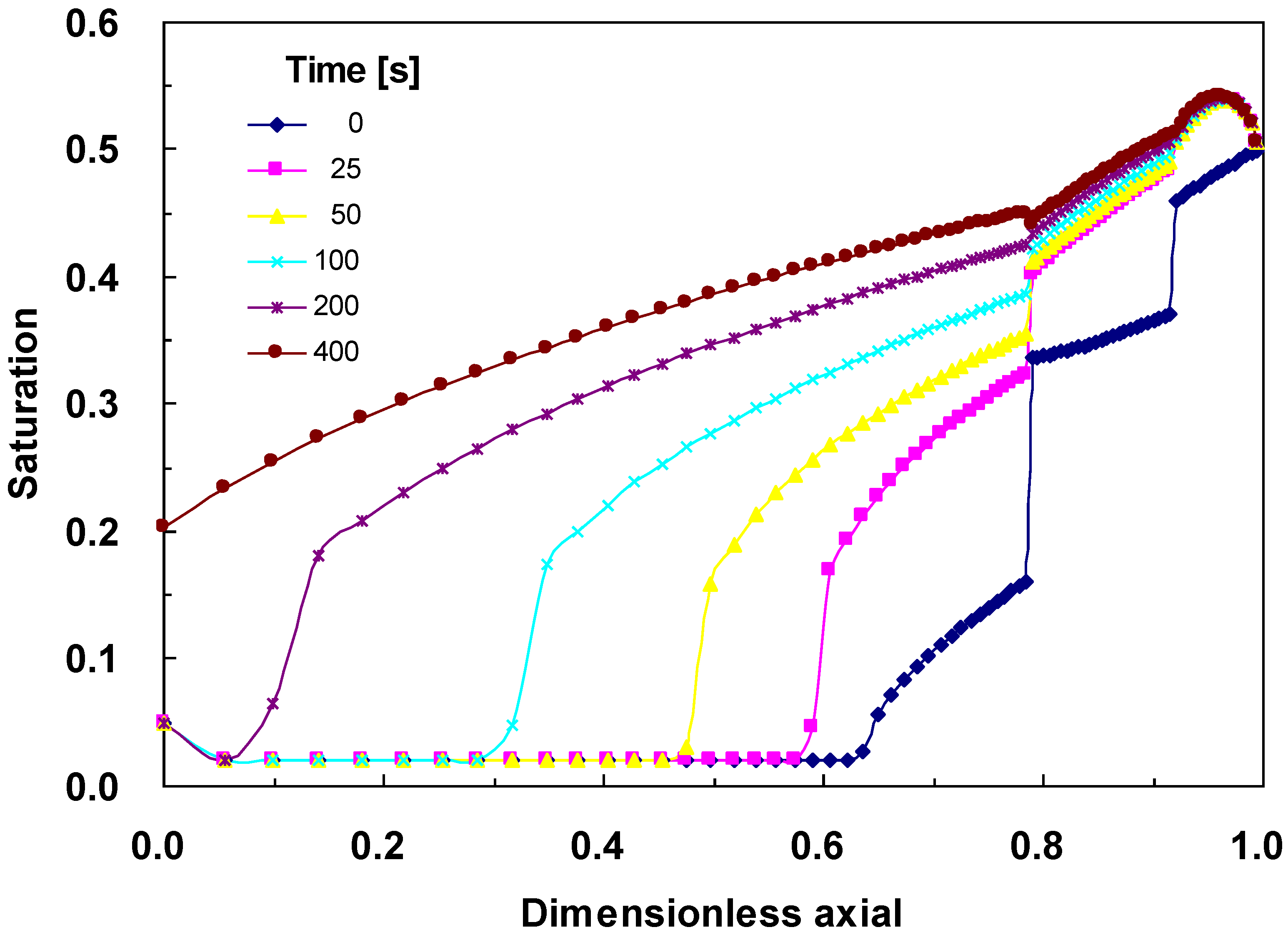
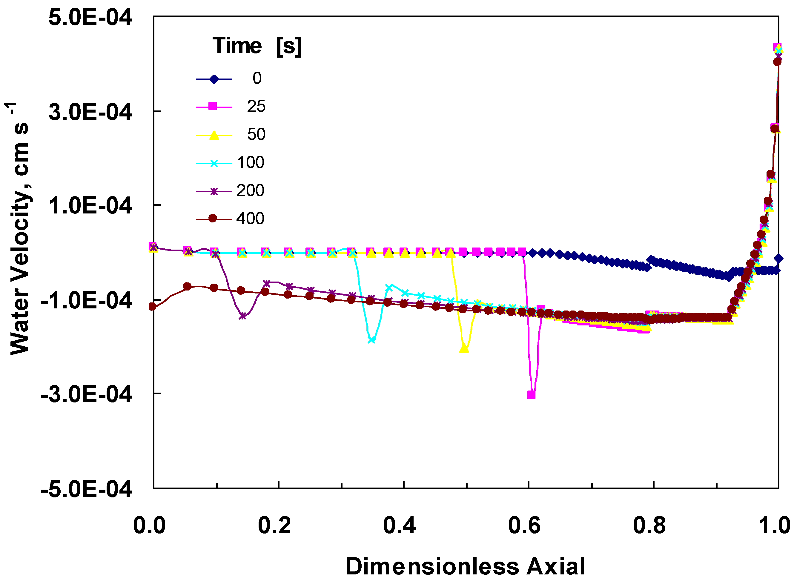
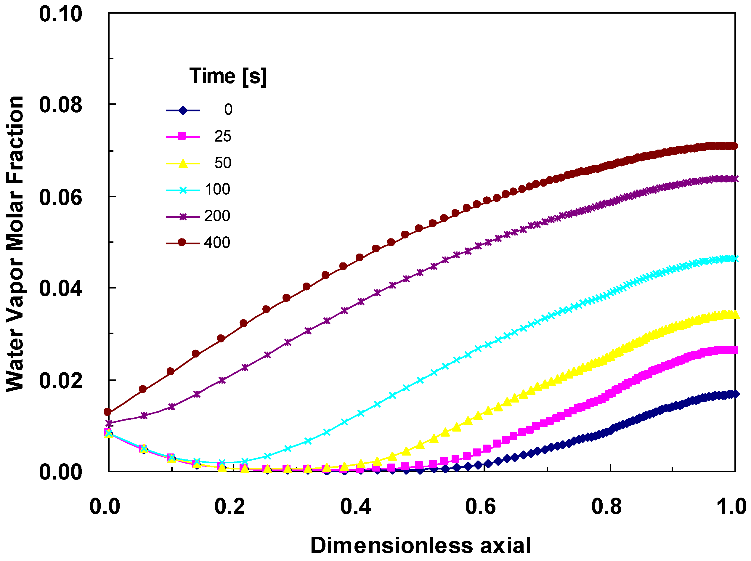
4.1. Overall Behavior

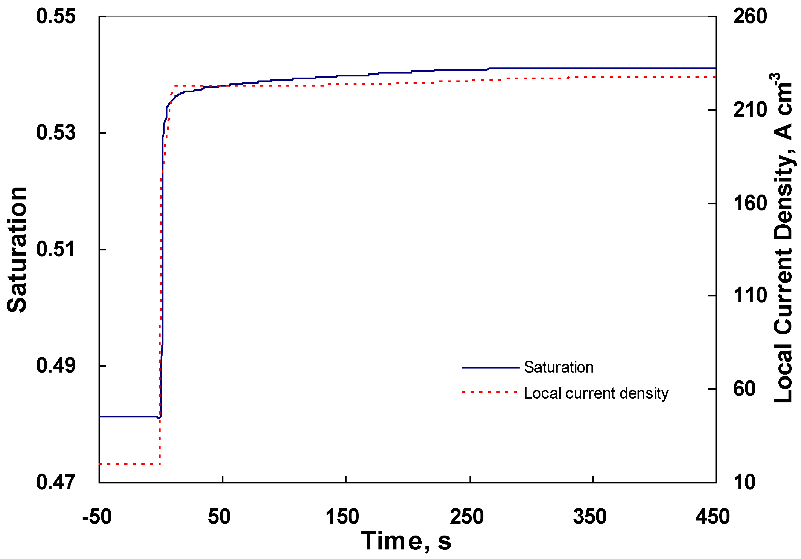
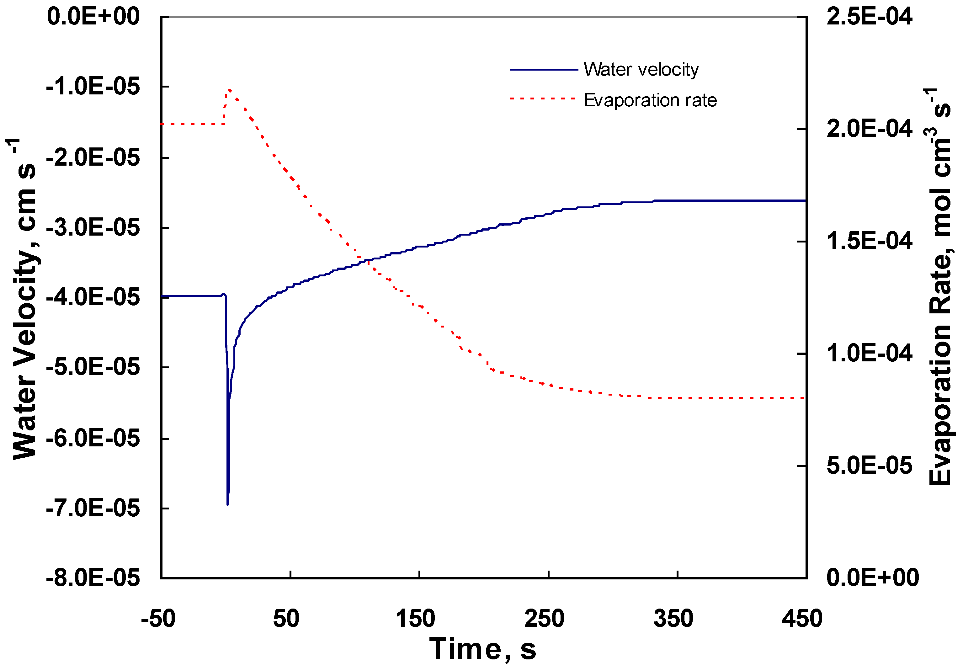
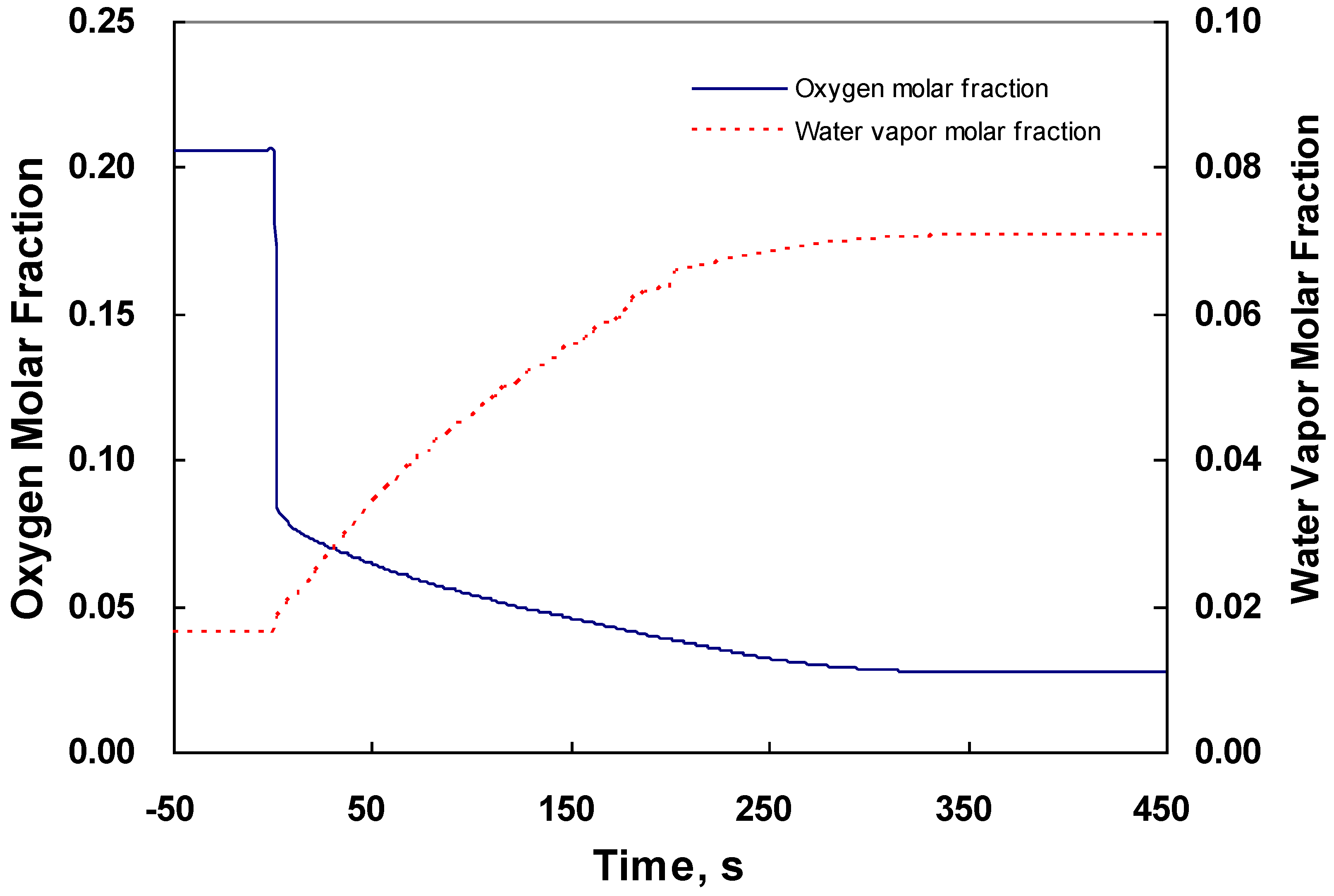
4.2. Dynamic Behavior in the Middle of the CL


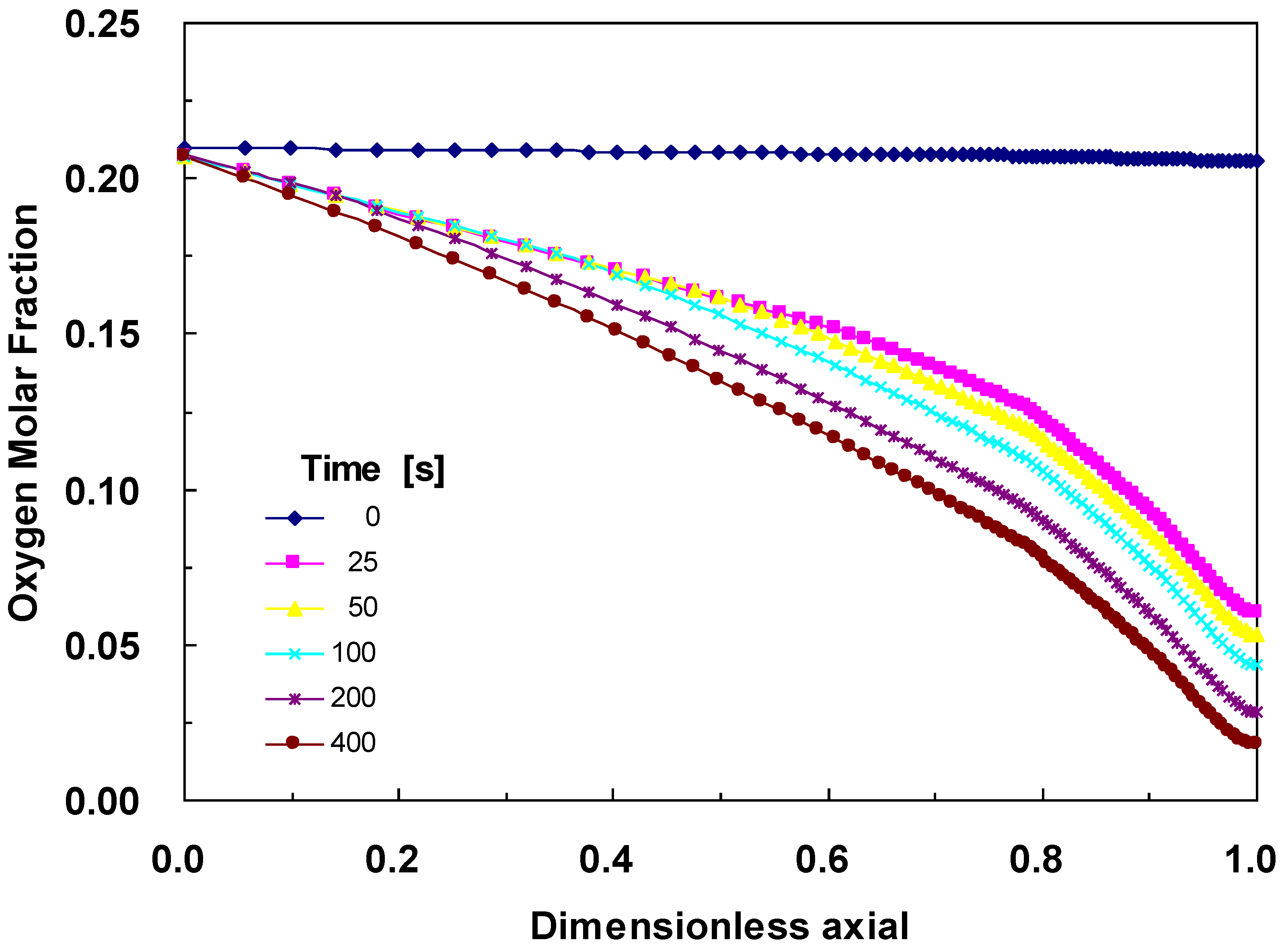
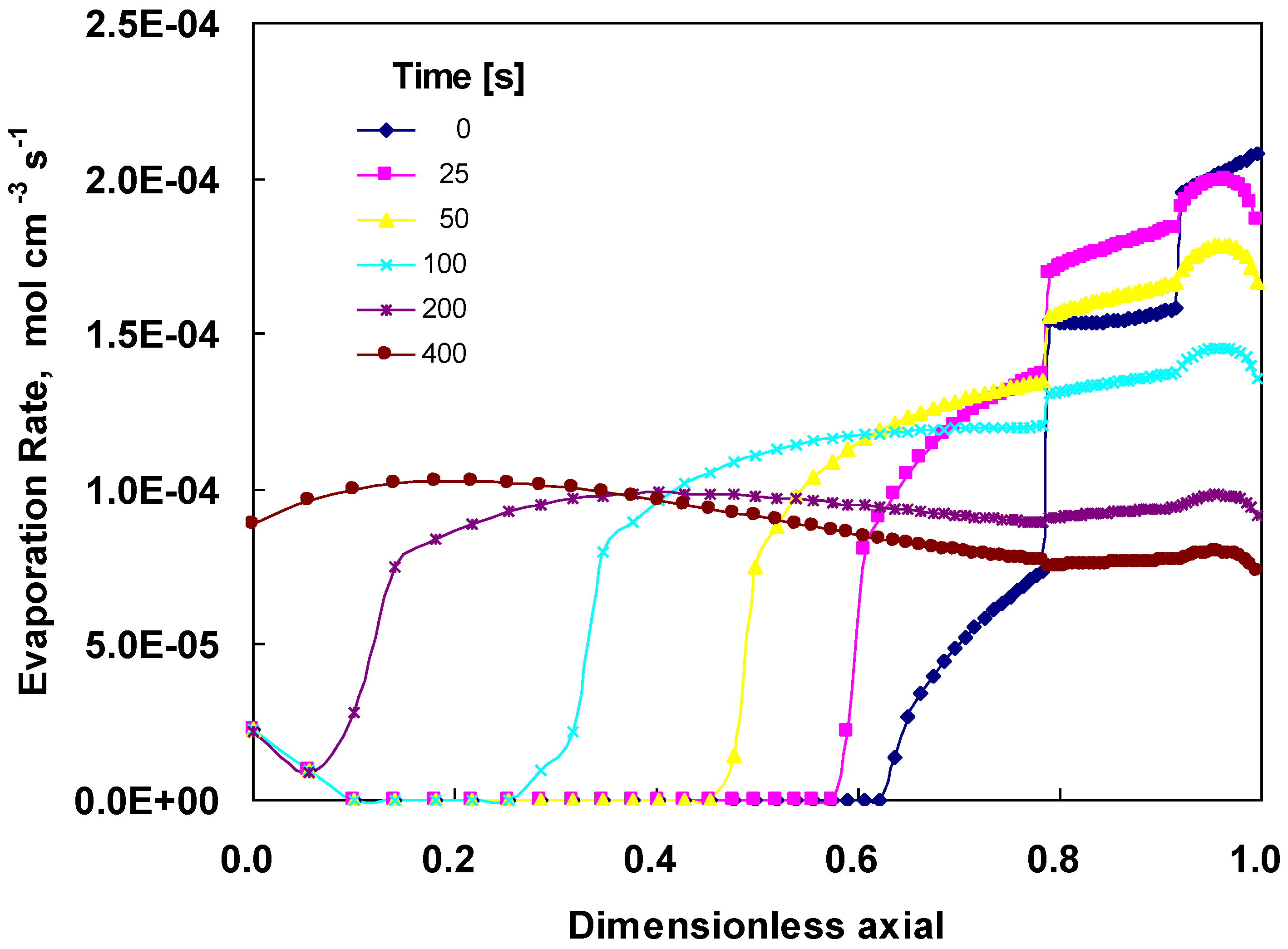
4.3. Changes across the Entire Cathode


5. Conclusions
Acknowledgment
References and Notes
- He, W.; Yi, J.S.; Nguyen, T.V. Two-phase flow model of the cathode of PEM fuel cells using interdigitaled flow fields. AICHE 2000, 46, 2053–2064. [Google Scholar] [CrossRef]
- Weng, F.B.; Su, A.; Hsu, C.Y.; Lee, C.Y. Study of water-flooding behavior in cathode channel of transparent proton-exchange membrane fuel cell. J. Power Sourc. 2006, 157, 674–680. [Google Scholar] [CrossRef]
- Zhan, Z.; Xiao, J.; Pan, M.; Yuan, P.R. Characteristics of droplet and film water motion in the flow channels of polymer electrolyte membrane fuel cells. J. Power Sourc. 2006, 160, 1–9. [Google Scholar] [CrossRef]
- Natarajan, D.; Nguyen, T.V. A two-dimensional, two-phase, multicomponent, transient model for the cathode of proton exchange membrane fuel cell using convention gas distributors. J. Electrochem. Soc. 2001, 148, A1324–1335. [Google Scholar] [CrossRef]
- Kong, C.S.; Kim, D.-Y.; Lee, H.-K.; Shul, Y.-G.; Lee, T-H. Influence of pore-size distribution of diffusion layer on mass-transport problems of proton exchange membrane fuel cell. J. Power Sourc. 2002, 108, 185–191. [Google Scholar] [CrossRef]
- Natarajan, D.; Nguyen, T.V. Three-dimensional effects of liquid water flooding in the cathode of a PEM fuel cell. J. Power Sourc. 2003, 115, 66–80. [Google Scholar] [CrossRef]
- Pisani, L.; Murgia, G.; Valentini, M.; D’Aguanno, B. A working model of polymer electrolyte fuel cells comparisions between theory and experiments. J. Electrochem. Soc. 2002, 149, A898–904. [Google Scholar] [CrossRef]
- Weber, A.Z.; Newman, J. Transport in polymer-electrolyte membranes I. Physical model. J. Electrochem. Soc. 2003, 150, A1008–A1015. [Google Scholar] [CrossRef]
- Weber, A.Z.; Newman, J. Transport in polymer-electrolyte membranes II. Mathematical model. J. Electrochem. Soc. 2004, 151, A311–A325. [Google Scholar] [CrossRef]
- Weber, A.Z.; Newman, J. Transport in polymer-electrolyte membranes III. Model validation in a simple fuel-cell model. J. Electrochem. Soc. 2004, 151, A326–A339. [Google Scholar] [CrossRef]
- Springer, T.E.; Zawodzinski, T.A.; Gottesfeld, S. Polymer electrolyte fuel cell model. J. Electrochem. Soc. 1991, 138, 2334–2342. [Google Scholar] [CrossRef]
- Um, S.; Wang, C.-Y.; Chen, K.S. Computational fluid dynamics modeling of proton exchange membrane fuel cells. J. Electrochem. Soc. 2000, 147, 4485–4493. [Google Scholar] [CrossRef]
- Hsing, I-M.; Futerko, P. Two-dimensional simulation of water transport in polymer electrolyte fuel cells. Chem. Eng. Sci. 2000, 55, 4209–4218. [Google Scholar] [CrossRef]
- Kulikovsky, A.A. Quasi-3D modeling of water transport in polymer electrolyte fuel cell. J. Electrochem. Soc. 2003, 150, A1432–1439. [Google Scholar] [CrossRef]
- Mazumder, S.; Cole, J.V. Rigorous 3-D mathematical modeling of PEM fuel cells I. Model predictions with liquid water transport. J. Electrochem. Soc. 2003, 150, A1503–1509. [Google Scholar] [CrossRef]
- Um, S.; Wang, C.-Y. Three-dimensional analysis of transport and electrochemical reactions in polymer electrilyte fuel cell. J. Power Sourc. 2004, 125, 40–51. [Google Scholar] [CrossRef]
- Mazumder, S. A generalized phenomenological model and database for transport of water and current in polymer electrolyte membranes. J. Electrochem. Soc. 2005, 152, A1633–1644. [Google Scholar] [CrossRef]
- Um, S.; Wang, C.-Y. Computational study of water transport in proton exchange membrane fuel cells. J. Power Sourc. 2006, 156, 211–223. [Google Scholar] [CrossRef]
- Weber, A.Z.; Newman, J. Effects of microporous layers in polymer electrolyte fuel cell. J. Electrochem. Soc. 2005, 152, A677–A688. [Google Scholar] [CrossRef]
- Pasaogullari, U.; Wang, C.-Y.; Chen, K.S. Two-phase transport in polymer electrolyte fuel cells with bilayer cathode gas diffusion media. J. Electrochem. Soc. 2005, 152, A1574–A1582. [Google Scholar] [CrossRef]
- Biyikoglu, A. Review of proton exchange membrane fuel cell models. Int. J. Hydrogen Energy 2005, 30, 1181–1212. [Google Scholar] [CrossRef]
- Baschuk, J.J.; Li, X. Modeling of polymer electrolyte membrane fuel cells with variable degrees of water flooding. J. Power Sourc. 2000, 86, 181–196. [Google Scholar] [CrossRef]
- Udell, K.S. Heat transfer in porous media heated from above with evaporation, condensation, and capillary effects. J. Heat Tran. 1983, 105, 485–492. [Google Scholar] [CrossRef]
- Pasaogullari, U.; Wang, C.-Y. Liquid water transport in gas diffusion layer of polymer electrolyte fuel cells. J. Electrochem. Soc. 2004, 151, A399–406. [Google Scholar] [CrossRef]
- Weber, A.Z.; Darling, M.; Newman, J. Modeling two-phase behavior in PEFCs. J. Electrochem. Soc. 2005, 151, A1715–A1727. [Google Scholar] [CrossRef]
- Yan, W.-M.; Soong, C.-Y.; Chen, F.; Chu, H.-S. Transient analysis of reactant gas transport and performance of PEM fuel cells. J. Power Sourc. 2005, 143, 48–56. [Google Scholar] [CrossRef]
- Chen, F.; Chu, H.-S.; Soong, C.-Y.; Yan, W.-M. Effective schemes to control the dynamic behavior of the water transport in the membrane of PEM fuel cell. J. Power Sourc. 2005, 140, 243–249. [Google Scholar] [CrossRef]
- Wang, Y.; Wang, C.-Y. Transient analysis of polymer electrolyte fuel cells. Electrochim. Acta 2005, 50, 1307–1315. [Google Scholar] [CrossRef]
- Shimpalee, S.; Spuckler, D.; Van Zee, J.W. Prediction of transient response for 25-cm2 PEM fuel cell. J. Power Sourc. 2007, 167, 130–138. [Google Scholar] [CrossRef]
- Patankar, S.V. Numerical Heat Transfer and Fluid Flow; Hemisphere Publishing Corporation: New York, NY, USA, 1980. [Google Scholar]
- Hirt, C.W.; Nichols, B.D. Volume of fluid (VOF) method for the dynamic of free boundaries. J. Comput. Phys. 1981, 39, 201–225. [Google Scholar] [CrossRef]
- Qi, Z.; Kaufman, A. Improvement of water management by a microporous sublayer for PEM fuel cells. J. Power Sourc. 2002, 109, 38–46. [Google Scholar] [CrossRef]
- Bernardi, D.M.; Verbrugge, M.W. Mathematical model of a gas diffusion electrode bonded to a polymer electrolyte. AICHE 1991, 37, 1151–1163. [Google Scholar] [CrossRef]
© 2010 by the authors; licensee MDPI, Basel, Switzerland. This article is an open-access article distributed under the terms and conditions of the Creative Commons Attribution license (http://creativecommons.org/licenses/by/3.0/).
Share and Cite
Chan, D.-S.; Hsueh, K.-L. A Transient Model for Fuel Cell Cathode-Water Propagation Behavior inside a Cathode after a Step Potential. Energies 2010, 3, 920-939. https://doi.org/10.3390/en3050920
Chan D-S, Hsueh K-L. A Transient Model for Fuel Cell Cathode-Water Propagation Behavior inside a Cathode after a Step Potential. Energies. 2010; 3(5):920-939. https://doi.org/10.3390/en3050920
Chicago/Turabian StyleChan, Der-Sheng, and Kan-Lin Hsueh. 2010. "A Transient Model for Fuel Cell Cathode-Water Propagation Behavior inside a Cathode after a Step Potential" Energies 3, no. 5: 920-939. https://doi.org/10.3390/en3050920