Energy Recovery for the Main and Auxiliary Sources of Electric Vehicles

Abstract

Based on the traditional regenerative braking electrical circuit, a novel energy recovery system for the main and auxiliary sources of electric vehicles (EVs) has been developed to improve their energy efficiency. The electrical circuit topology is presented in detail. During regenerative braking, the recovered mechanical energy is stored in both the main source and the auxiliary source at the same time. The mathematical model of the proposed system is derived step by step. Combining the merits and defects of H₂ optimal control and H_∞ robust control, a H₂/H_∞ controller is designed to guarantee both the system performance and robust stability. The perfect match between the simulated and experimental results validates the notion that the proposed novel energy recovery system is both feasible and effective, as more energy is recovered than that with the traditional energy recovery systems, in which recovered energy is stored only in the main source.

1. Introduction

In a world where environmental protection and energy conservation are growing concerns, the development of electric vehicles (EVs) as potential ecological transportation tools has taken on an accelerated pace [1]. However, the commercialization and popularization of EVs has not been very successful. Of all the technological challenges facing EVs, their high initial cost and short driving range remain the main barriers to success. Energy recovery is an efficient approach to extending the driving range with limited energy sources, and the driving range of EVs could be increased 25–30% [2]. For example, the “Prius” EV from the Toyota Company can extend its driving range by up to 20% with regenerative braking energy, and the “Insight” EV from Honda can increase it by 30% [3], but the energy recovery efficiency is not the highest [4]. Multiple storage devices consisting of batteries and peak-power sources are proposed to improve the energy efficiency of conventional EVs. Flywheels and supercapacitors seem to be suitable as peak-power sources. The recovered energy is charged to the peak-power source or the main source through a DC/DC converter working as a booster [5,6]. In general, the rated voltage of peak-power sources is much higher than the bus level, which is defined by the main source (batteries). As a result, the DC/DC converter has to boost the back Electro-Motive-Force (EMF) of the motor to the voltage of the peak-power source. The higher the voltage of the main source is, the more difficult it is for the DC/DC converter to provide this boost. When the EMF of the motor decreases too low to boost to the voltage of the main source, the rotating mechanical energy is consumed by circuit resistances as thermal energy, which is wasted. If the wasted energy can be recovered, the energy recovery efficiency can be further improved. For most EVs, electrical components are powered by the main source through a DC/DC converter. The power requirements of the electrical components have been rising rapidly for many years and are expected to continue to rise. These increasing power requirements are the main cause for the short driving ranges of EVs, which prevent EVs from further commercialization. Some EVs, however, are conversions from traditional internal combustion engine (ICE) cars, for example the GM EV1 [1]. A traditional auxiliary source is reserved to power the electrical components instead of a DC/DC converter. The voltage of the auxiliary source is 12 V or 24 V, which is much lower than the bus level [7]. When the EMF of the motor is too low to boost to the voltage of the main source, it is higher than the voltage of the auxiliary source, so the energy can be recovered further by an electrical circuit working as a bucker.

In most traditional energy recovery systems, the recovered mechanical energy is only stored at the main source or peak-power source of EV, which consists of a single battery pack or is coupled to supercapacitors or flywheels. In this paper, a novel energy recovery system for the main and auxiliary sources is presented. During regenerative braking, the recovered energy is stored both at the main source and the auxiliary source. There have been no reports on the circuit topology of the proposed system until now. The control of the proposed system is complicated by its nonlinear characteristics and unknown environmental parameters. Various attempts to satisfy the control performance for traditional energy recovery systems have been presented, such as variable structure control in [8], fuzzy control in [9], intelligent control in [10,11], and neural network control [12]. However it should be noted that these aforementioned controllers are all based on a fairly concise model, where the uncertainty is not considered. H₂/H_∞ control has been proven to be effective for controls related to nonlinear dynamic systems [13], so H₂/H_∞ control is applied for the novel energy recovery system for the main and auxiliary sources.

In this paper, the scheme and principles of the novel energy recovery system are presented, emphasizing first on the electrical circuit topology. Then the mathematical model is derived step by step. Aimed at addressing the strong nonlinear characteristics of the proposed novel energy recovery system, a H₂/H_∞ controller is designed to guarantee both the system performance and robust stability. Subsequent to a simulation of the system and some experiments, the paper discusses in detail the feasibility and effectiveness of the proposed system. Finally, the conclusions are summarized.

2. Energy Recovery System for the Main and Auxiliary Sources

2.1. The Scheme and Principle

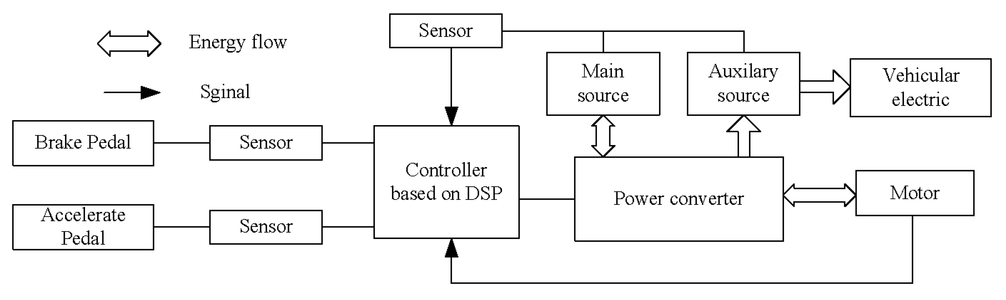
The case study is carried out on the “XJTUEV_II” EV, which was converted from an ICE car by Xi’an Jiaotong University and the auxiliary source was preserved. A schematic of the energy recovery system for the main and auxiliary sources of the “XJTUEV_II” EV is depicted in Figure 1. It consists of the main source, the auxiliary source, the controller, the power converter and the DC motor. The main source provides the storage energy for traction of the motor, formed by a pack of 10 lead-acid batteries (12 V, 245 Ah). The auxiliary source, formed by a lead-acid battery (12 V, 60 Ah), provides the energy for the electrical vehicular components. The nominal voltage of the DC motor is 120 V. During driving, the motor current refers to the sensor voltage of the accelerator pedal. According to the reference current, the main source provides the energy to the motor and propels the vehicle. During regenerative braking, the charging currents to the main and auxiliary sources refer to the sensor voltage of the brake pedal. Both the main and auxiliary sources store the recovered energy. Occasionally the storage energy of the auxiliary source is deficient, and then the main source delivers energy to it by the power converter. Thus the auxiliary source doesn’t need an additional charger. Compared with the traditional regenerative braking system, which stores the recovered energy at the main source only, the proposed energy recovery system stores the energy both at the main and auxiliary sources and more energy is thus recovered.

Figure 1. The schematic of the energy recovery system for the main and auxiliary sources.

Figure 1. The schematic of the energy recovery system for the main and auxiliary sources.

2.2. The Electrical Circuit

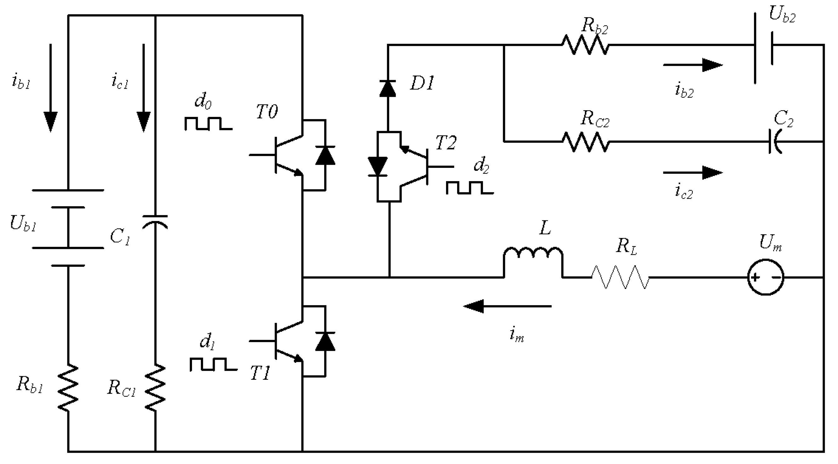
The electrical circuit of the novel energy recovery system is depicted in Figure 2, where L and R_L are the inductance and resistance of the motor armature; U_b1 and U_b2 are the voltage of the main and auxiliary sources; C₁ and C₂ are the filter capacitor of the main and auxiliary sources; i_m is the current passing through the motor armature; i_b1 and i_{b2 ,} i_c1 and i_c2 are the currents passing through the main and auxiliary sources and corresponding filter capacitors, respectively; U_m is the voltage of the EMF of the motor armature; d₁ and d₂ are the duty cycle of IGBT T1 and T2, R_b1, R_c1, R_b2, R_c2 are the wire resistances. The power converter consists of IGBT T1, T2, and T0. The power converter works in a boost converter or buck converter mode. Through the power converter the energy can flow from the main source to the traction motor, the recovered energy can flow from the motor to the main and auxiliary sources at the same time, and the energy can flow from the main source to the auxiliary source [14]. What is important is that the diode D1 is necessary. Without D1, the auxiliary source will be short-circuiting when T1 switches on. The current is along U_b2→T2→T1→U_b2.

Figure 2. The electrical circuit of the system.

Figure 2. The electrical circuit of the system.

During driving, T1 and T2 switch off, and T0 switches on PWM mode. The power converter works as a bucker. The traction current of the motor depends on the duty cycle of PWM T0. The traction current is along the main source→T0→the motor, as shown in Figure 3a. Once the energy of the auxiliary source is deficient, which seldom happens, the main source begins to charge the auxiliary source. T2 or T0 switches on PWM mode, and the other switches on. T1 switches off all the time. The charging current is along the main source→T0→T2→ the auxiliary source, as shown in Figure 3b.

Figure 3. (a)The currents during the driving; (b) The charging current from the main source to the auxiliary source.

Figure 3. (a)The currents during the driving; (b) The charging current from the main source to the auxiliary source.

During the braking, the rotating motor can’t stop suddenly because of its mechanical inertia and tends to rotate in the original direction. The EMF of the motor armature continues to hold its magnitude and polarity, the motor works in an energy resuming braking mode and a regenerative braking mode alternatively.

2.2.1. Energy Resuming Braking Mode

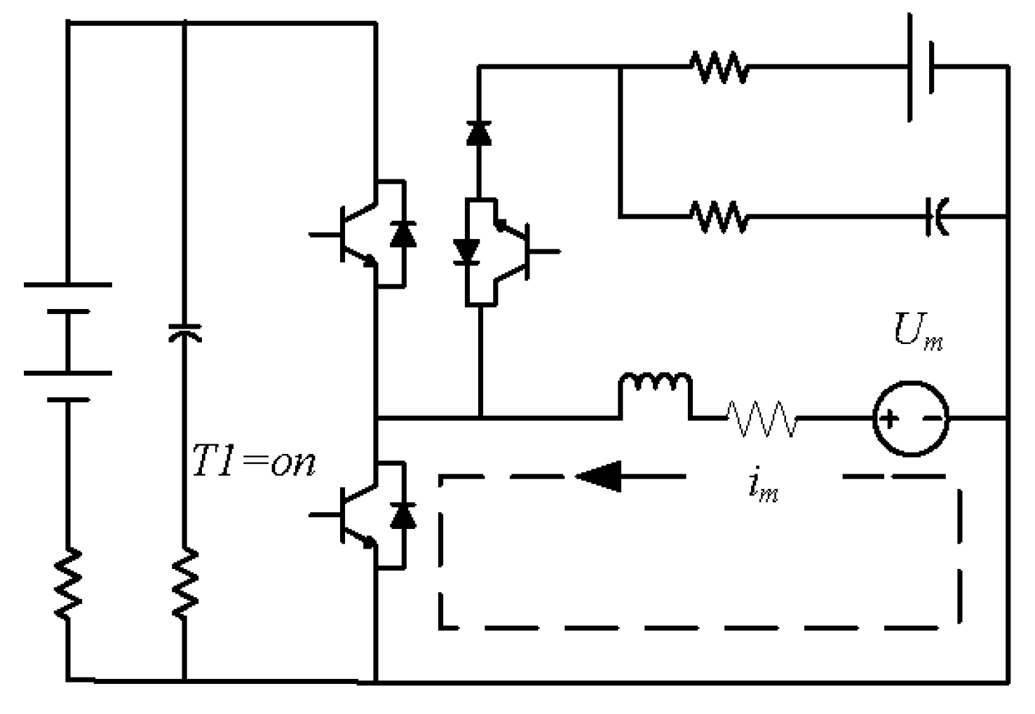
During the energy resuming braking mode, both T2 and T0 switch off, and T1 switches on. The current is motivated by the EMF of the motor. With the increase of the motor current, the inductance of the motor armature begins to store the energy. The current is along the positive polarity of EMF→T1→the negative polarity of EMF, which is shown in Figure 4. As the direction of the motor current is inverted to the traction current, the motor generates braking torque to decelerate the vehicle.

Figure 4. The currents during the energy resuming brake.

Figure 4. The currents during the energy resuming brake.

2.2.2. Regenerative Braking Mode

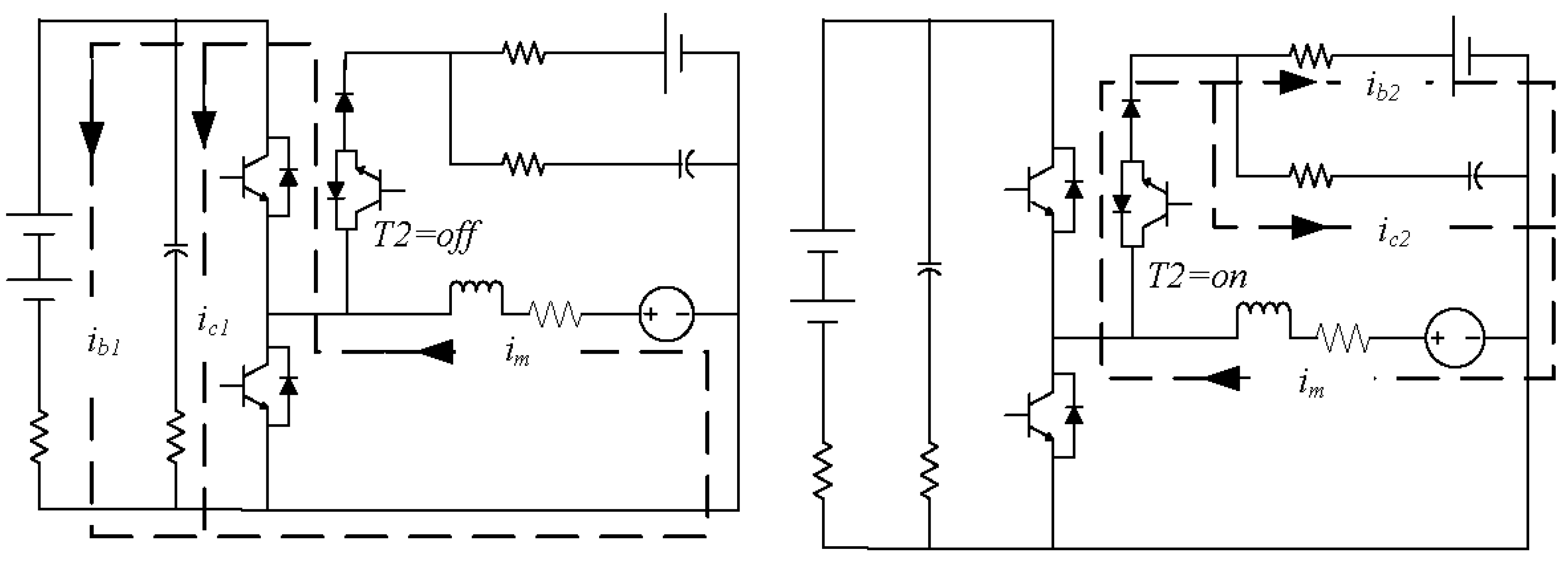
During the regenerative braking, the storage energy of the motor armature inductance is delivered to the main and auxiliary sources. Firstly all IGBTs T1, T2 and T0 switch off. Because the current of the motor armature can’t disappear suddenly, the inductance begins to pump the storage energy to the main source by the power converter working as a booster. The current is along the positive polarity of EMF→T0→the main source → the negative polarity of EMF, which is shown in Figure 5a. The value of the charging current to the main source depends on the duty cycle of PWM T1.

Figure 5. (a) The charging current to the main source; (b) The charging current to the auxiliary source.

Figure 5. (a) The charging current to the main source; (b) The charging current to the auxiliary source.

When the voltage of the EMF is not high enough to boost to the voltage of the main source, IGBT T2 switches on. The inductance begins to deliver the energy to the auxiliary source by the power converter working as a bucker. The current is along the positive polarity of EMF→T2→ the auxiliary source→the negative polarity of EMF, which is shown in Figure 5b. The value of the charging current to the auxiliary source depends on the duty cycle of PWM T2.

2.3. The Mathematic Model

Taking the currents of Figure 2 as the normal direction, the electrical circuit of the system can be characterized by the following sets of equations (1–3). During braking, T0 switches off all the time. During the energy consuming braking, T1 switches on, and T2 switches off. The circuit equations can be expressed by [15]:

$$\begin{array}{l}L\frac{\mathrm{d}{i}_m}{\mathrm{d}t}=U_m-R_L{i}_m\\ C_1\frac{\mathrm{d}{U}_{C1}}{\mathrm{d}t}=\frac{U_{C1}-U_{b1}}{R_{b1}+R_{C1}}\\ C_2\frac{\mathrm{d}{U}_{C2}}{\mathrm{d}t}=\frac{U_{C2}-U_{b2}}{R_{b2}+R_{C2}}\end{array}$$

(1)

During the regenerative braking, the recovered energy is stored first at the main source. Both T1 and T2 switch off. The circuit equations can be expressed by:

$$\begin{array}{l}L\frac{\mathrm{d}{i}_m}{\mathrm{d}t}=U_m-R_L{i}_m-\frac{U_{b1}-U_{C1}+i_m*R_{b1}}{R_{C1}+R_{b1}}{R}_{C1}-U_{C1}\\ C_1(R_{b1}+R_{C1})\frac{\mathrm{d}{U}_{C1}}{\mathrm{d}t}=U_{b1}-U_{C1}+i_m*R_{b1}\\ C_2\frac{\mathrm{d}{U}_{C2}}{\mathrm{d}t}=\frac{U_{C2}-U_{b2}}{R_{b2}+R_{C2}}\end{array}$$

(2)

During the regenerative braking, the recovered energy is stored secondly at the auxiliary source. T1 switches off, and T2 switches on. The circuit equations can be expressed by:

$$\begin{array}{l}L\frac{\mathrm{d}{i}_m}{\mathrm{d}t}=U_m-R_L{i}_m-\frac{U_{b2}-U_{C2}+i_m*R_{b2}}{R_{C2}+R_{b2}}{R}_{C2}-U_{C2}\\ C_1\frac{\mathrm{d}{U}_{C2}}{\mathrm{d}t}=\frac{U_{C1}-U_{b1}}{R_{b1}+R_{C1}}\\ C_2(R_{b2}+R_{C2})\frac{\mathrm{d}{U}_{C2}}{\mathrm{d}t}=U_{b2}-U_{C2}+i_m*R_{b2}\end{array}$$

(3)

Selecting the state vector of the electrical circuit as $x={[\begin{array}{ccccc}{i}_m& & U_{C1}& & U_{C2}\end{array}]}^{\mathrm{T}}$, where i_m is the current passing through the motor armature, U_C1 the voltage of the main filter capacitor, and U_C2 the voltage of the auxiliary filter capacitor. Selecting the control vector as $u={[\begin{array}{ccccc}{U}_m& & U_{b1}& & U_{b2}\end{array}]}^{\mathrm{T}}$, where U_m, U_b1 and U_b2 are the voltages of the EMF of the motor, the main and auxiliary sources, and the output vector as $y={[\begin{array}{ccc}{i}_{b1}& & i_{b2}\end{array}]}^{\mathrm{T}}$, where i_b1 is the charging current to the main source and i_b2 the charging current to the auxiliary source [16]. Then the system can be transformed to the state equations (4, 5, 6) corresponding to the circuit equations (1–3).

The state equation corresponds to equation (1) is:

$$\begin{array}{l}\dot{x}=A_{1}x+B_{11}u\\ y=C_{1}x+D_{11}u\end{array}$$

(4)

The state equation corresponds to equation (2) is:

$$\begin{array}{l}\dot{x}=A_{2}x+B_{12}u\\ y=C_{2}x+D_{12}u\end{array}$$

(5)

The state equation corresponds to equation (3) is:

$$\begin{array}{l}\dot{x}=A_{3}x+B_{13}u\\ y=C_{3}x+D_{13}u\end{array}$$

(6)

where the coefficient matrices refer to Appendix I. The matrices of the state equations (4-6) are defined by the electrical circuit of the “XJTUEV_II” EV. The corresponding coefficients are as follows: L = 0.139 mH, R_L = 0.0118 Ω, C₁ = 4*470 μF, C₂ = 470 μF, R_b1, R_c1, R_b2, R_c2 are approximately 0.1 Ω. We synthesize the equations (4-6) by $(4)\times d_1+(5)\times (1-d_1-d_2)+(6)\times d_2$, where d₁ is the duty cycle of PWM T1, and d₂ is the duty cycle of PWM T2. The synthesized system is not continuous, but nonlinear. It is difficult to design a controller based on a nonlinear model. Because the modulation frequency of PWM is 20 kHz, it is much higher than the crossover frequency of the electrical circuit of the system [17]. According to the state space averaging method and small-signal assumption [17], the system behavior can be described by the following small-signal equations:

$$\begin{array}{l}\dot{\tilde{x}}=A^{*}\tilde{x}+B_1^{*}\tilde{u}+B_2^{*}\tilde{w}\\ \tilde{y}=C^{*}\tilde{x}+D_1^{*}\tilde{u}+D_2^{*}\tilde{w}\end{array}$$

(7)

where $\tilde{x}={[\begin{array}{ccccc}{\tilde{i}}_m& & {\tilde{U}}_{C1}& & {\tilde{U}}_{C2}\end{array}]}^{\mathrm{T}}$, and $\tilde{u}={[\begin{array}{ccc}{\tilde{d}}_1& & {\tilde{d}}_2\end{array}]}^{\mathrm{T}}$, are the averaged state vectors and input vectors respectively, $\tilde{y}={[\begin{array}{ccc}{\tilde{i}}_{b1}& & {\tilde{i}}_{b2}\end{array}]}^{\mathrm{T}}$, is the averaged output vector. $\tilde{w}={[\begin{array}{ccccc}{\tilde{U}}_M& & {\tilde{U}}_{b1}& & {\tilde{U}}_{b2}\end{array}]}^{\mathrm{T}}$, is the averaged disturbance vector. The signal ‘~’ means the perturbation from a steady-state working point (X’, U’), where X’ and U’ are the state and control vector. The coefficient matrix refers to Appendix I. According to the reference data and calculation, the steady state working point can be set as that $d_1^{\prime }=0.25,d_2^{\prime }=0.15$, $i_m^{\prime }=45\text{A},V_{c1}^{\prime }=125\text{V},V_{c2}^{\prime }=12.5\text{V}$ during the braking for EV“XJTUEV_II”. Then the coefficient matrices of state space equation (7) are calculated as:

$$A^{*}=\left[\begin{array}{ccc}436.7& -2343.8& -585.9\\ 159.6& -531.9& 0\\ 159.6& 0& 744.6\end{array}\right]B_1^{*}=\left[\begin{array}{ccc}7812.5& -2343.8& -585.9\\ 0& 531.9& 0\\ 0& 0& -744.6\end{array}\right]B_2^{*}=\left[\begin{array}{cc}97656& 85078\\ -1064& -1064\\ 0& 8085\end{array}\right]$$

$$C^{*}=\left[\begin{array}{ccc}0.3& 5& 0\\ 0.07& 0& 5\end{array}\right]D_1^{*}=\left[\begin{array}{ccc}0& -5& 0\\ 0& 0& -5\end{array}\right]D_2^{*}=\left[\begin{array}{cc}-40& -40\\ 0& 0\end{array}\right]$$

(8)

3. H₂/H_∞ Control

“XJTUEV_II” EV was converted from an ICE car and retained its gear box and cluster. First, because the braking system is composed of mechanical braking and electrical braking, the variation of the strength of mechanical braking is a serious disturbance to the control system. Secondly, since the converted EV reserves the gear box and the cluster, the variation of the driving style leads to the variation of the inertia moment equalling to the motor shaft from the chassis weight, resulting in the perturbation of the model parameter. Thirdly the stochastic variation of the battery voltage and the rolling resistance are uncertainty elements for the model. On the other hand, the DC/DC converter is a strongly nonlinear system for the inherent PWM modulation method [18]. Combining the merits and deficiencies of H₂ optimal control and H_∞ robust control, H₂/H_∞ controller is provided to guarantee both the system performance and the robust stability of the system. A model in terms of state space equation is denoted as:

$$\begin{array}{l}\dot{x}=Ax+B_{1}u+B_{2}w\\ z_1=C_{1}x+D_{11}u+D_{12}w\\ z_2=C_{2}x+D_{21}u+D_{22}w\end{array}\}$$

(9)

where $x$ is the state vector, $u$ is the control input vector, $w$ is the outer disturbance vector, $z_1$ and $z_2$ are the control output vector, and $A,B_1,B_2,C_1,C_2,D_{11},D_{12},D_{21}$ and $D_{22}$ are certain known matrices defined by the nominal model. H₂/H_∞ controller to be designed should guarantee that 1)the closed-loop system is stable; 2) the performance index for robustness satisfies that ${\Vert T(z_{1}w)\Vert }_{\infty }<{\gamma }_1$ with the parameter perturbation and outer disturbance, defined by the H_∞ norm of the transfer function $T(z_{1}w)$ from $w$ to $z_1$. 3) the performance index for Linear Quadratic Gaussian(LQG) is as small as possible satisfying that ${\Vert T(z_{2}u)\Vert }_2<{\gamma }_2$, defined by the H₂ norm of the transfer function $T(z_{2}u)$ from $u$ to $z_2$. The design of the controller means to minimize ${\gamma }_2$ with the situation of $\sigma (K)\subset C^{-}$, ${\Vert T_{z_{1}w}\Vert }_{\infty }<{\gamma }_1,{\Vert T_{z_{2}u}\Vert }_2<{\gamma }_2$, where K is the controller to be designed [19].

The state vector of the proposed energy recovery system is $x={[\begin{array}{ccccc}{i}_m& & U_{C1}& & U_{C2}\end{array}]}^{\mathrm{T}}$, which are defined as the current of the motor and the voltages of the main and auxiliary sources. All the state variables can be measured directly by a physical sensor. So the state feedback controller is feasible. Design the state feedback controller as:

$$u=Kx$$

(10)

Substituting equation (10) into equation (9), rewrites the equation as:

$$\begin{array}{l}\dot{x}=(A+B_{1}K)x+B_{2}w\\ z_1=(C_1+D_{11}K)x+D_{12}w\\ z_2=(C_2+D_{21}K)x+D_{22}w\end{array}\}$$

(11)

The H₂/H_∞ controller design for equation (11) is difficult because of the solution of the nonlinear matrix inequality. According to the variable substitution method in [20], the state feedback controller is solvable with the existence of the optimal solution X,W of equation (12). The H₂/H_∞ controller can be expressed as $u=W{X}^{-1}x$:

$$\begin{array}{l}\min {\gamma }_2\\ s.t.\{\begin{array}{l}\left[\begin{array}{ccc}AX+B_{1}W+{(AX+B_{1}W)}^T& B_2& {(C_{1}X+D_{11}W)}^T\\ B_2^T& -{\gamma }_{1}I& D_{12}\\ C_{1}X+D_{11}W& D_{22}& -{\gamma }_{1}I\end{array}\right]<0\\ AX+B_{1}W+{(AX+B_{1}W)}^T+B_2{B}_2^T<0\\ \left[\begin{array}{cc}-Z& C_{2}X+D_{21}W\\ {(C_{2}X+D_{21}W)}^T& -X\end{array}\right]<0\\ Trace(Z)<{\gamma }_2\end{array}\end{array}$$

(12)

For the “XJTUEV_II”EV, $z_1=[\omega ]$ is defined as the angular velocity of the motor, which is proportional to the EMF. $z_2={[\begin{array}{cc}{i}_{b1}& i_{b2}\end{array}]}^{\mathrm{T}}$ are defined as the reference charging currents to the main and auxiliary sources, which is the ratio to the sensor voltage corresponding to the angular displacement of the brake pedal. Now we define the performance index for robustness as the H_∞ norm of the sensitivity function from the parameter perturbation $w$ to the control output z₁ And we define the performance index for LQG as the H₂ norm of the transfer function from the control input $u$ to the control output z₂. Thus, the coefficient matrices of equation (9) are $C_2=0,D_{21}=E_2,D_{22}=0$ for the braking system of the “XJTUEV_II” EV, the other matrices are $A=A^{*},B_1=B_1^{*},B_2=B_2^{*}$ $,C_1=C^{*},$ $D_{11}=D_1^{*},$ $D_{12}=D_2^{*}$ corresponding to equation (8). The design of the robust H₂/H_∞ controller is equal to the convex optimization of the linear objective function within the linear matrix inequality restriction. The designed controller is as follows by MATLAB/LMI toolbox:

$$K=\left[\begin{array}{ccc}-0.7994& -0.1406& 1.1199\\ -0.6048& -0.2426& -1.4860\end{array}\right]$$

(13)

The state feedback controller can guarantee that the H₂ performance index is ${\Vert T(z_{2}u)\Vert }_2<24$ and the H_∞ performance index ${\Vert T(z_{1}w)\Vert }_{\infty }<20$.

4. Simulation of the Energy Recovery System

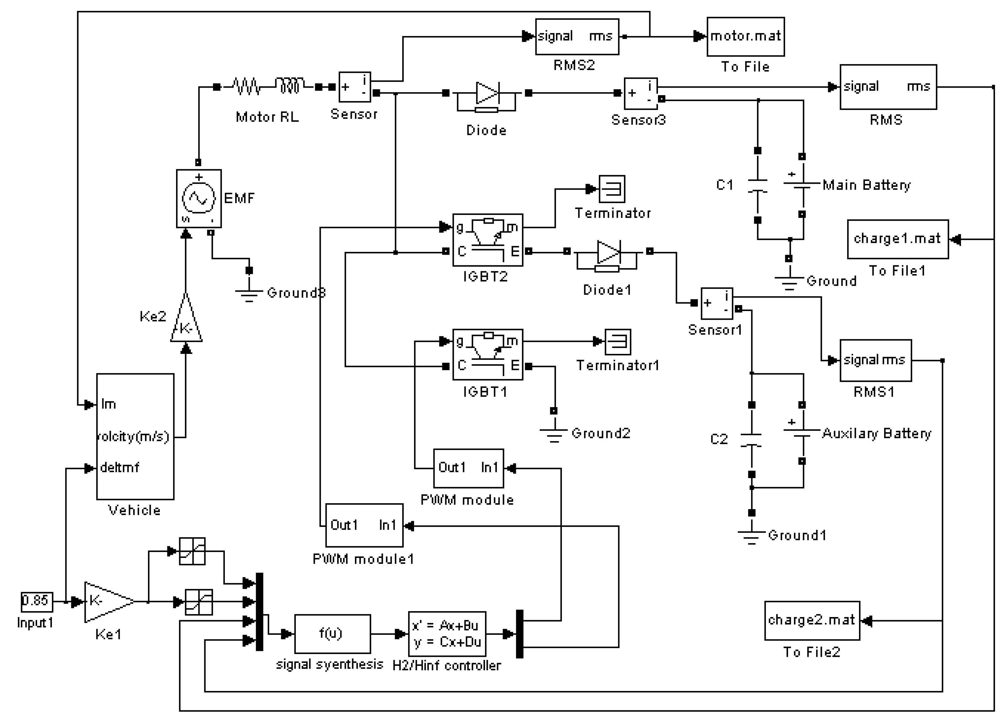
Based on the MATLAB/PSB toolbox, the simulation model of the energy recovery system for the main and auxiliary sources is shown in Figure 6. The input of the model was the sensor voltage of the brake pedal. For simplicity, the reference value was normalized. Then it multiplied the proportional coefficient $K_{e1}=200$ and $K_{e2}=40$ as the real charging currents to the main and auxiliary sources. According to the state of charge of a lead-acid battery, the maximum charging current can’t exceed 15% of the battery content, so the charging current to the main source was limited to 40 A, and the current to the auxiliary source was limited to 12 A. The output of the model was taken as the current of the motor armature, the charging currents to the main and auxiliary sources, respectively. In Figure 6, the “vehicle” module presents the dynamics model of EV, whose input was the braking torque deciding by the brake pedal and the electro-magnetic torque of the motor, the output was the angular velocity of the motor reflecting the EMF of the motor [21]. The “H2/Hinf controller” block was the state feedback controller corresponding to the equation (13). During braking, T0 switches off all the time, so it can be expressed as a “diode”.

Figure 6. The simulation model of the proposed energy recovery system.

Figure 6. The simulation model of the proposed energy recovery system.

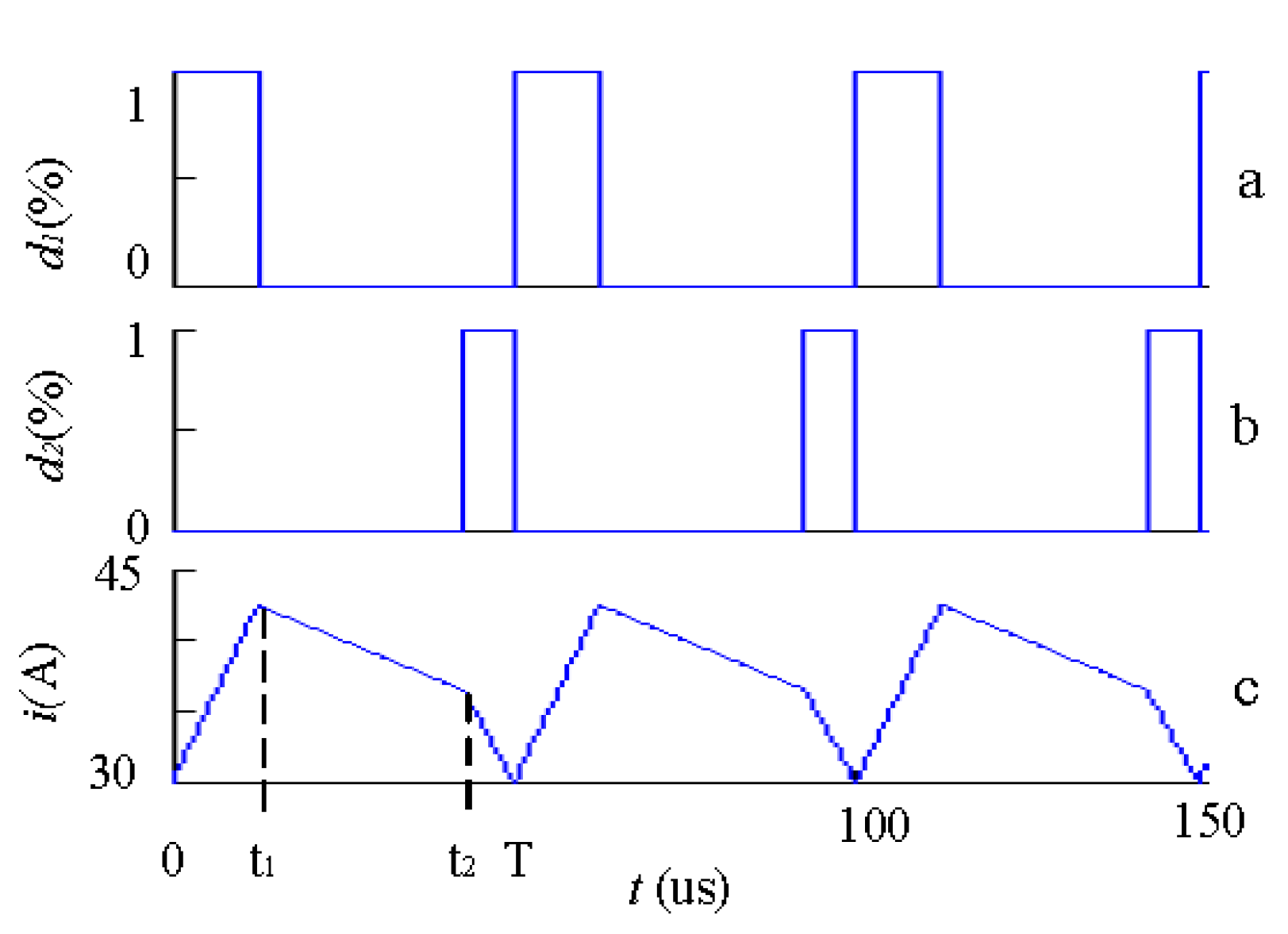
The modulated frequency of PWM was 20 kHz, and the microcurrent curves in one period are shown at Figure 7. The PWM T1 is shown at Figure 7a. Figure 7b presents the PWM of T2, and Figure 7c shows the motor current. During the interval [0 t₁], the motor worked in the energy consuming braking mode. The current passing through the motor armature began to increase and the inductance of the motor armature stored the energy. During the interval [t₁ t₂], the motor worked first in the regenerative braking mode. The storage energy of the motor armature was pumped to the main source. During the interval [t₂ T], the stored energy was secondly delivered to the auxiliary source. Then another alternative period began. The charging currents to the main and auxiliary sources could be adjusted by the duty cycle of d₁ and d₂, respectively.

Figure 7. The PWM and current of the circuit at one period.

Figure 7. The PWM and current of the circuit at one period.

Then the simulation was carried out at the root-mean-square (RMS) signal of the model, and the macro simulated results are shown in Figure 8 and Figure 9. In Figure 8 the comparative research was conducted between the traditional energy recovery system and the proposed energy recovery system.

Figure 8. (a) The charging current for the main source only; (b) The charging currents for both the main and auxiliary sources.

Figure 8. (a) The charging current for the main source only; (b) The charging currents for both the main and auxiliary sources.

The traditional system stored the recovered energy at the main source only. However the proposed system stored the recovered energy both at the main source and the auxiliary source. Figure 8a shows the charging current of the traditional system, and Figure 8b shows the charging currents of the proposed system. The input normalized values of the simulated model were 0.85 for both the systems. The simulated results show that the charging currents of the two systems rose to their maximum limitation quickly, and the response time was about 0.02 s. Then the motor currents still rose to keep the charging currents at the reference value. The H₂/H_∞ controller was endowed with high performance in accuracy, stability, and rapidity. At about 0.9 s the EMF of the motor was not high enough to boost to the voltage of the main source, so the charging current to the main source began to descend. However for the proposed system the EMF was high enough to buck to the voltage of the auxiliary source, so the charging current to the auxiliary source still reached its maximum limit. At 1.05 s the EMF of the motor was not high enough to charge the auxiliary source. The charging current to the auxiliary source began to descend until the motor stopped. The comparative results showed that with the same initial velocity of the EV for braking, the braking time were basically same for both the systems. The recovered energy for the main sources of the two systems were both nearly 4,800 J, but the additional auxiliary source of the proposed system recovered 158 J more energy, so the energy efficiency of the proposed system was improved nearly 3%.

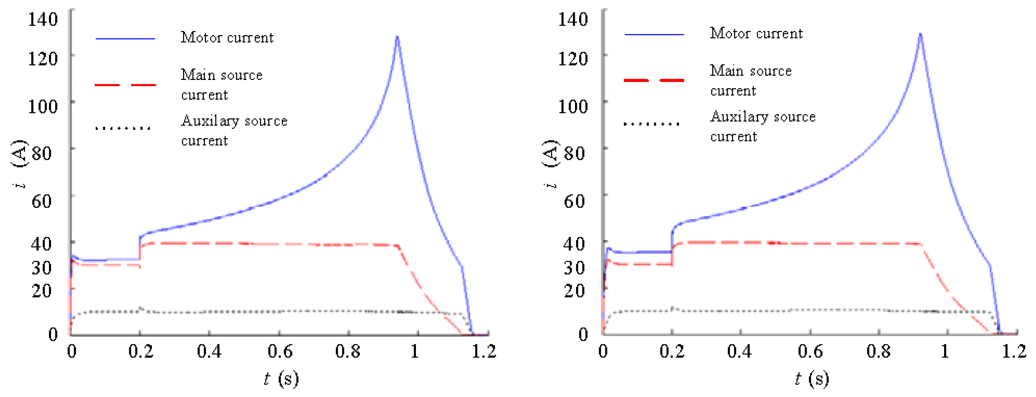
The step responses of the simulated models for the proposed system are shown is Figure 9. To test the performance of the controller with the outer disturbance and the parameter perturbation, comparative simulations were carried out on the nominal model and the perturbation model of the proposed system. The inputs of the models were both 0.15 first, and stepped to 0.3 at 0.2 s. The input step was equaled to the step of the braking torque, which was a disturbance for the system. The charging currents of the nominal model are shown in Figure 9a, and Figure 9b shows the perturbation model. For the nominal model the voltage of the main source was 120 V and the auxiliary source 12 V. For the perturbation system the voltage of the main source was 144 V and the auxiliary source 14 V. It can be concluded from the simulated results that with the same parameters, the charging power increased with the perturbation of the voltage of the sources resulting in the raising of the motor current. However the state feedback controller for the proposed system can guarantee both the system performance and robust stability with the parameter perturbation and the outer disturbance.

Figure 9. (a) The step response for the nominal model; (b) The step response for the perturbation model.

Figure 9. (a) The step response for the nominal model; (b) The step response for the perturbation model.

5. Experimental Results

5.1. The Hardware Design of the DSP-based Controller

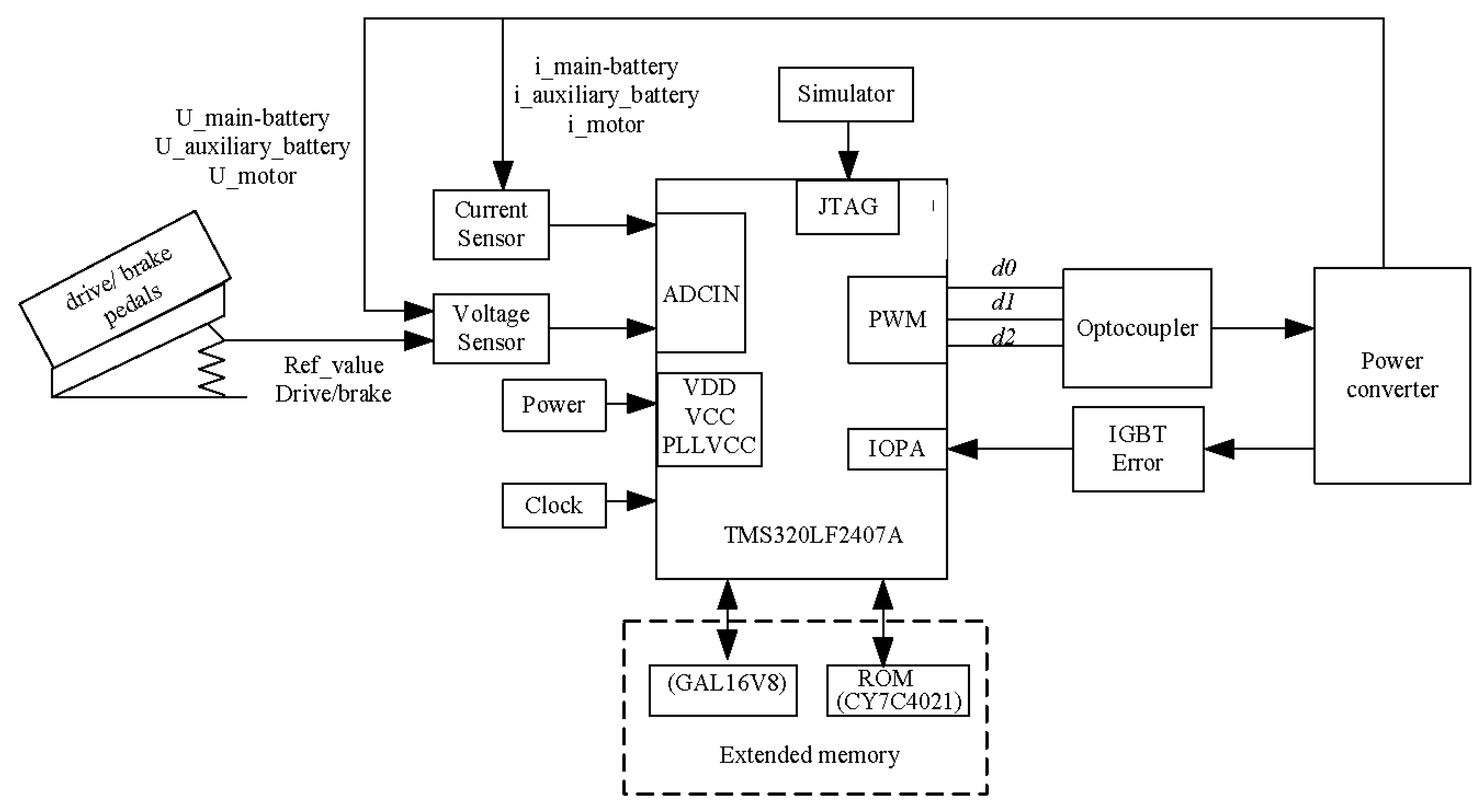
The configuration of the hardware controller is shown in Figure 10. The main processor of the experimental system was a DSP TMS320LF2407A with a clock frequency of 40 MHz. The currents were detected by the Hall-effect sensor (LEM208) and the detected analog signals were converted to digital values by using a A/D converter with a 12-bit resolution. The energy from the auxiliary source supplied the core processor. The drive reference value, the brake reference value, the bidirectional motor current, the bidirectional battery current, the voltage of power source, and the additional analogy signals can be acquainted by the current and voltage sensor and adjusted by the filter circuit. The output PWM provided the drive signals for IGBT, and controlled the conducting time of the power devices. I/O module received the error signals from the driver board of IGBT, and turned on the corresponding diode to alarm.

Figure 10. The configuration of the controller hardware.

Figure 10. The configuration of the controller hardware.

5.2. The Software Program of the DS-based Controller

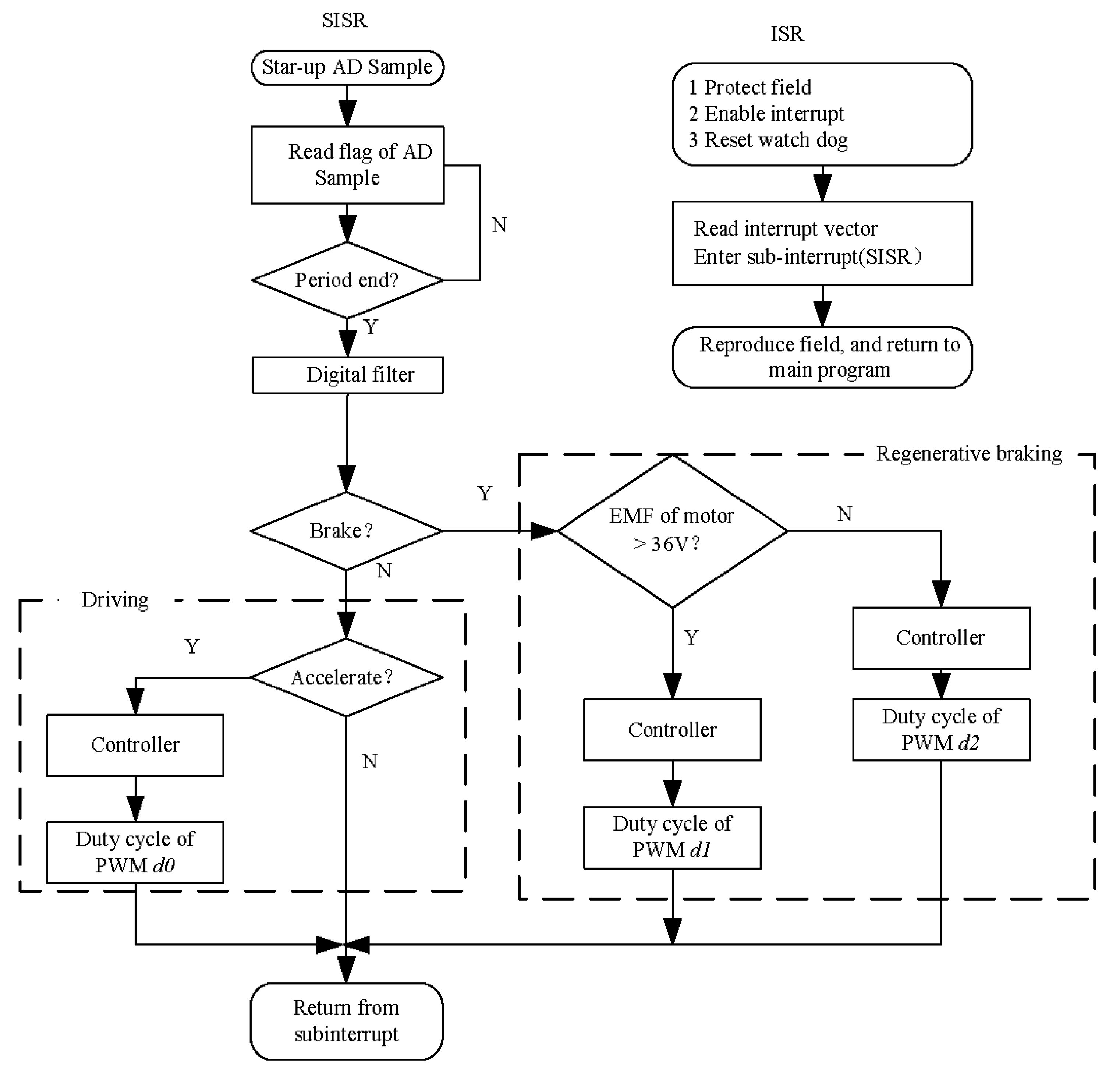
The sampling period of the proposed control scheme was 50 μs. The state feedback controller designed by MATLAB was rewritten in C language and loaded into the on-board memory of the TMS320LF2407 system board. The flowchart of the main program is shown in Figure 11. After resetting the DSP, the main program began with the initialization, which included the declaration of the head file of A/D, PWM, I/O modules. All the registers were cleared and the interrupt vector was loaded for the interrupt service routine. If all jobs were ready, enable the interrupt and wait for the timer cycle interrupt. Once the cycle interrupt happened, the main program jumped to the interrupt service routine. The modulation frequency was 20 kHz.

The control processing was performed by two subroutines: ISR performed the job of field protection and interrupt arbiter and SISR executed the data acquaints and current control. SISR read the measured currents from the A/D converter and calculated the duty cycle of PWM, which was interrupted at a sampling rate 20 kHz. As a result of the current regulation, the voltage of obtained and used for the PWM signals was generated. The controller first responded to the brake reference input for safety, which meant that once both the drive and brake pedals gave out the inputs by wrong action or outside disturbance, the controller performed the braking job, and the vehicle stayed still. During regenerative braking, when the EMF of the motor was more than 36 V, the controller sent out the duty cycle d1 of PWM T1. When it was less than 36 V, then the duty cycle d2 was sent out.

Figure 11. The configuration of the controller software.

Figure 11. The configuration of the controller software.

5.3. Experiments

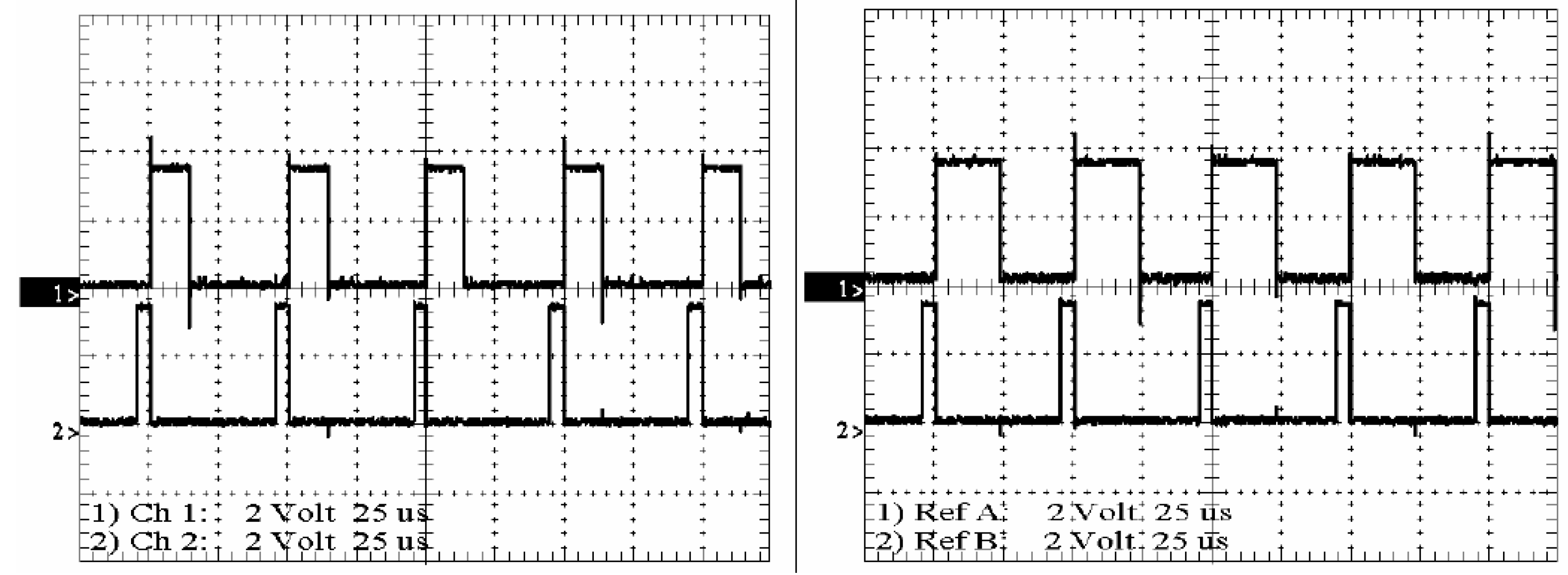
To validate the feasibility and effectiveness of the energy recovery system, experiments were carried out for the “XJTUEV_II” EV in the emergent and soft brake modes. The experiments were focused on the current control of the system. The current curve was acquired with a Tektronix oscilloscope. In Figure 12, Figure 13 and Figure 14, the results on the left correspond to experiments in soft brake mode, and the right column to emergent mode. Figure 12 shows the PWM waveform of the DSP. Figure 13 shows the current of the motor winding corresponding to Figure 12. Figure 14 shows the RMS signals of the currents of the motor and the sources. First, a micro experiment was carried out, and the resulting PWM is shown in Figure 12. In Figure 12a and Figure 12b, the first channel shows the PWM of T1, and the second channel shows the PWM of T2. When the system was stable in a soft brake mode, the duty cycle of the PWM T1 was 25%, and T2 was 10%. When the system was stable in an emergent brake mode, the duty cycle of the PWM T1 was 50%, and T2 was 10%.

Figure 12. (a)The PWM waveform at soft brake; (b) The PWM waveform at emergent brake.

Figure 12. (a)The PWM waveform at soft brake; (b) The PWM waveform at emergent brake.

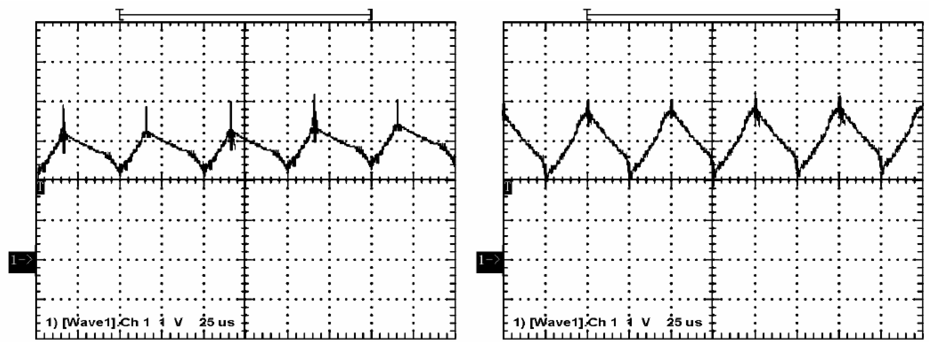
With the constraint of only two channels of Tektronix oscilloscope TEK2010, the motor currents corresponding to Figure 12 are shown in Figure 13. The motor current began to increase when T1 was switched on, then decreased when T1 was switched off. When T2 switched on, the rate of decrease was accelerated. The experimental results were in agreement with the simulated results in Figure 7.

Figure 13. (a) The motor current at soft brake; (b) The motor current at emergent brake.

Figure 13. (a) The motor current at soft brake; (b) The motor current at emergent brake.

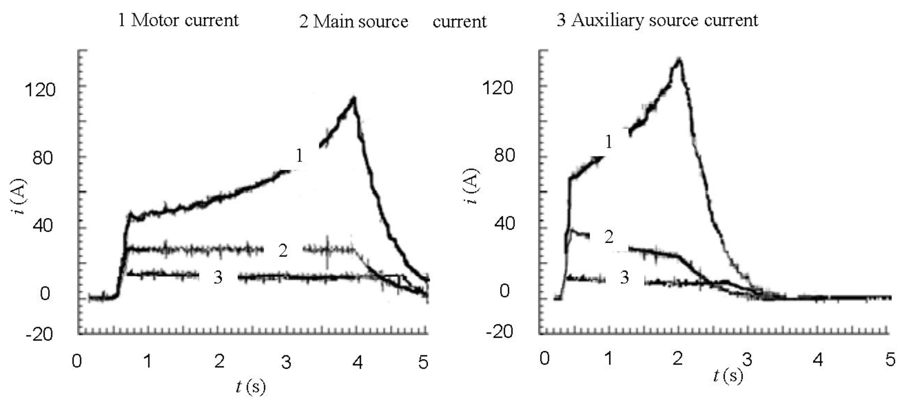
From Figure 14, it can be concluded that the charging current to both the main and auxiliary source was stable, with quick response and minor stability issues. In the emergent brake mode, the charging current to the main source can’t hold the maximum value and begins to descend with overshoot. However, the charging current to the auxiliary source was good. The experimental results were in agreement with the simulated results. In soft brake mode the recovered energies were 16,800 J and 576 J for the main and auxiliary source, respectively, and the energy efficiency was improved 3%. In emergent brake mode the recovered energies were 6,000 J and 360 J, and the energy efficiency was improved by 6%.

Figure 14. (a) the RMS currents at a soft brake mode; (b) the RMS currents at an emergent brake mode.

Figure 14. (a) the RMS currents at a soft brake mode; (b) the RMS currents at an emergent brake mode.

The experimental results show that the electrical circuit of the energy recovery system can work as a boost-buck converter. It can make the inductance of the motor pump the current to the main source and charge the auxiliary source at the same time. The simulated and experimental results showed that the current can be controlled, which validates the effectiveness and the feasibility of the proposed energy recovery system.

6. Conclusions

The traditional methodology for the regenerative braking of EV was extended in depth, and a novel energy recovery system for the main and auxiliary sources was presented. The H₂/H_∞ controller for the proposed system was designed. Comparative simulations were carried on the traditional and novel energy recovery systems. The simulation and experimental results showed that the proposed system is both feasible and effective, and recovers more energy during the braking of EVs. The designed controller can guarantee both the system performance and robust stability when faced with parameter perturbation and outer disturbances.

The vehicular electrical components are critical in the safety, comfort and maneuverability of a vehicle [7]. Safety standards require the auxiliary source to be continuously working. If the main source is discharged essential, the electrical components won't function for the traditional EV powering the electrical components through a DC/DC converter. It's less like to happen with the auxiliary source supplying the loads independently, for the auxiliary source can support the electrical loads in normal driving with the regenerative braking energy, which is presented in this paper. The proposed system can be widely applied to battery EVs, hybrid EVs and fuel cell EVs, to improve the energy efficiency and lengthen the driving range of these vehicles.

References

- Chan, C.C. The State of the Art of Electric, Hybrid, and Fuel Cell Vehicles. Proc. IEEE 2007, 95, 704–718. [Google Scholar] [CrossRef]
- Cao, B.G.; Zhang, C.W.; Bai, Z.F. Trend of development of technology for electric vehicles. J. Xi’an Jiaotong Univ. 2004, 389, 1–5. [Google Scholar]
- Henry, K.N.; John, A.A. Engine Start Characteristics of Two Hybrid Electric Vehicles (HEVS)-Honda Insight and Toyota Prius; SAE: Detroit, MI, USA, 2001. [Google Scholar]
- Chuang, Y.; Chau, K.T. Thermoelectric automotive waste heat energy recovery using maximum power point tracking. Energy Convers. Manage. 2009, 50, 1506–1512. [Google Scholar] [CrossRef]
- Burke, A.F. Batteries and Ultracapacitors for Electric, Hybrid, and Fuel Cell Vehicles. Proc. IEEE 2007, 95, 806–820. [Google Scholar] [CrossRef]
- Phatiphat, T.; Stephane, R.; Bernard, D. Energy management of fuel cell/battery/supercapacitor hybrid power source for vehicle applications. J. Power Sources 2009, 193, 376–385. [Google Scholar] [CrossRef]
- Xu, Z. Current progress and strategy study on the vehicular electric industry. Ind. Technol. Economy 2006, 125, 106–108. [Google Scholar]
- Chung, S.K. Robust speed control of brushless direct-drive motor using integral variable structure control. IEE Proc. Electr. Power Appl. 1995, 142, 361–370. [Google Scholar] [CrossRef]
- Paterson, J.; Ramsay, M. Electric vehicle braking by fuzzy logic control. Proc. IEEE IASAM 1993, 3, 2200–2204. [Google Scholar]
- Cholula, S.; Claudio, A.; Ruiz, J. Intelligent Control of the Regenerative Braking in an Induction Motor Drive; ICEEE: Mexico City, Mexico, 2005; pp. 302–308. [Google Scholar]
- Lennon, W.K.; Passino, K.M. Intelligent control for brake systems. IEEE Trans. Contr. Syst. Technol. 1999, 7, 188–202. [Google Scholar] [CrossRef]
- Gao, H.; Gao, Y.; Ehsani, M. A neural network based SRM drive control strategy for regenerative braking in EV and HEV. In Proceedings of Electric Machines and Drives Conference, Cambridge, MA, USA, 17–20 June 2001.
- Bai, Z.F. H∞ robust control for driving and regenerative braking of electric vehicle. J. Xi’an Jiaotong Univ. 2005, 39, 256–260. [Google Scholar]
- Yan, X.; Patterson, D. Novel power management for high performance and cost reduction in an electric vehicle. Renewable Energy 2001, 22, 177–183. [Google Scholar] [CrossRef]
- Panagiotidis, M.; Delagrammatikas, G.; Assanis, D. Development and Use of a Regenerative Braking Model for a Parallel Hybrid Electric Vehicle; SAE: Detroit, MI, USA, 2000. [Google Scholar]
- HSAHA, S. A modified approach of feeding regenerative energy to the Main source. IEEE Trans. IE 1996, 43, 510–514. [Google Scholar]
- Paolo, M.; Leopoldo, R.; Giorgio, S. Small-signal analysis of DC-DC converters with sliding mode control. IEEE Trans. Power Electron. 1997, 12, 96–102. [Google Scholar] [CrossRef]
- Jesus, L.R.; Jorge, A.M.S. Uncertainty models for switch-mode DC-DC Converters. IEEE Trans. Circuits Syst. 2000, 47, 200–203. [Google Scholar] [CrossRef]
- Doyle, C.J.; Glover, K. State space solution to standard H2 and H∞ control problems. IEEE Trans. Autom. Control 1989, 34, 831–847. [Google Scholar] [CrossRef]
- Glover, K.; Mcfarlane, D. Robust stabilization of normalized coprime factor plant descriptions with H∞ bounded uncertainty. IEEE Trans. Autom. Control 1989, 34, 821–830. [Google Scholar] [CrossRef]
- Ye, M.; Bai, Z.F.; Cao, B.G. Robust Hybrid Control for Energy Recovery for Main and Auxiliary Sources of Electric Vehicle. In Proceedings of IEEE 2nd Conference on Industrial Electronics and Applications; IEEE CS Press: Harbin, China, 2007; pp. 896–901. [Google Scholar]
© 2010 by the authors; licensee MDPI, Basel, Switzerland. This article is an open access article distributed under the terms and conditions of the Creative Commons Attribution license (http://creativecommons.org/licenses/by/3.0/).
Share and Cite
MDPI and ACS Style
Ye, M.; Jiao, S.; Cao, B. Energy Recovery for the Main and Auxiliary Sources of Electric Vehicles. Energies 2010, 3, 1673-1690. https://doi.org/10.3390/en3101673
AMA Style
Ye M, Jiao S, Cao B. Energy Recovery for the Main and Auxiliary Sources of Electric Vehicles. Energies. 2010; 3(10):1673-1690. https://doi.org/10.3390/en3101673
Chicago/Turabian StyleYe, Min, Shengjie Jiao, and Binggang Cao. 2010. "Energy Recovery for the Main and Auxiliary Sources of Electric Vehicles" Energies 3, no. 10: 1673-1690. https://doi.org/10.3390/en3101673