Robust State of Charge Estimation for Hybrid Electric Vehicles: Framework and Algorithms

Abstract

State of Charge (SoC) estimation is one of the most significant and difficult techniques to promote the commercialization of electric vehicles (EVs). Suffering from various interference in vehicle driving environment and model uncertainties due to the strong time-variant property and inconsistency of batteries, the existing typical SoC estimators such as coulomb counting and extended Kalman filter cannot perform their theoretically optimal efficacy in practical applications. Aiming at enhancing the robustness of SoC estimation and improving accuracy under the real driving conditions with noises and uncertainties, this paper proposes a framework consisting of (1) an adaptive-κ nonlinear diffusion filter to reduce the noise in current measurement, (2) a self-learning strategy to estimate and remove the zero-drift, (3) a coulomb counting algorithm to realize open-loop SoC estimation, (4) an $H_{\infty }$ filter to implement closed-loop robust estimation, and (5) a data fusion unite to achieve the final estimation by integrating the advantages of the two SoC estimators. The availability and efficacy of each component have been demonstrated based on comparative studies in simulation with the conventional approaches respectively, under the testing conditions of noises with various signal-noise-ratios, varying zero-drifts, and different model errors. The overall framework has also been verified to rationally and efficiently combine these components and achieve robust estimation results in the presence of kinds of noises and uncertainties.

1. Introduction

Electric Vehicles (EVs), including pure electric vehicles and hybrid electric vehicles, are usually recognized as the solution to solve the problems of global energy crisis and environmental deterioration. To meet the requirements of EVs, batteries, as the alternative power source, have to be more powerful with high voltage and large capacity, and hence request for a multi-functional, reliable, intelligent and safe Battery Management System (BMS). Dickinson et al. even highlighted BMS as the probably single most important technical issue in the successful commercialization of EVs [1].

State of Charge (SoC), defined as the ratio of residual capacity to the nominal full capacity, is the most fundamental state of a battery, which functions as the “fuel gauge” for conventional fuel-driven vehicles. Unfortunately, the crucial state is not directly measurable, essentially requiring a soft estimator to calculate it. The accurate estimation result can indicate the amount of residual energy in a battery, inform users the left range, and cooperate with Vehicle Management System (VMS) to prolong battery life cycle and achieve the overall optimal energy efficiency. Therefore, SoC estimation has attracted wide coverage in both researches and applications in the past decade, and becomes to one of the most significant but difficult issues in BMS design.

1.1. Literature Review

A comprehensive review of SoC estimation for general battery-powered applications has been studied by Valer Pop et al. [2]. However, limited by the special requirements for EV application, such as realtime estimation, avoidance of energy loss and forbiddance of injecting extra test signals during vehicle in-service period, some typical, usually more accurate, methods are impractical to estimate SoC of power battery in EV, for example Open Circuit Voltage (OCV) direct measurement, discharge test, measurement of electrolyte physical properties [3] and a.c. impedance spectroscopy [4,5].

Coulomb counting (usually denoted as Ah method) is one of the most applicable SoC indicators, which simply accumulates the charges transferred in or out of the battery. Recently, some advanced techniques have been proposed to enhance its performance by on-line estimating charege/discharge efficiencies [6,7]. Essentially, coulomb counting family is a kind of open-loop estimators which require accurate measurement of battery current. It will accumulate current noise and has no ability to self-correct. If the mean of noise is nonzero, i.e., in the presence of zero-drift, the estimation result even becomes to divergence.

Model-based methods also have been well studied, aiming at establishing a closed-loop estimation based on a battery model. Battery models usually apply current as model control input, terminal voltage as measured output, and SoC, State of Health (SoH) and/or equivalent OCV as hidden states [8,12]. Extended Kalman Filter (EKF) was firstly utilized to estimate these hidden states according to realtime sampling data of current and terminal voltage [13], and then further improved by enhancement strategies such as reduced order EKF [14], augmented states EKF [15], adaptive EKF [16] and Sigma-point KF [17,18]. To be an optimal estimator, EKF requires an accurate model and the knowledge on the statistic properties of noises. The two conditions actually cannot be achieved easily in the real vehicle running environment, because the strong time-variant property of battery make the difficulty of determining a battery model by a set of fixed parameters and the characteristics of measurement noises depend on vehicle driving conditions so that it is hard to obtain them beforehand. To overcome this problem, sliding model observer was utilized to compensate the modeling errors and uncertainties [19,20]. However, the selection of parameters in sliding model observer, such as boundaries of uncertainties and switching gains, still depends on the comprehensive understanding of battery dynamics. Moreover, a set of unsuitable parameters even has the risk of causing the chattering phenomena [20], leading to the unwanted vibration in SoC estimation.

To avoid the difficulty of battery modeling and identification, machine learning strategies were also introduced to establish black-boxes mapping measurable data to SoC, including Neural Network (NN) [21], fuzzy NN [22,23], evolutionary NN [24,25] and support vector machine [26,27]. These data-oriented methods can not avoid their intrinsic problems such as large number of training data covering the whole possible range of operation, the selection of model structure and the balance between under-fitting and over-fitting. Meanwhile, the estimation result is theoretically unpredictable when suffered from kinds of noises.

In recent years, some hybrid or combined estimation frameworks have been proposed to integrate the advantages of individual estimators with different characters. The combination of RC and hysteresis models was proposed to compensate deficiencies of the individual models [28]. Coulomb counting and EKF based estimation were integrated to achieve better performance [29,30,31]. An very accurate result that estimation error was less than 1 min in left time or 1% in SoC was also obtained under the together contributions of direct measurement of the electro-motive force and book-keeping algorithm [32], though it is not specially designed for EV application. The inspiring results reveal that establishment of SoC estimation frameworks which rationally consist of kinds of estimators is a potential way to achieve more accurate and robust performance.

1.2. Overview of Proposed Framework

The real vehicle driving environment often involves interference sources which cause signal measurement noises and even zero drift. Meanwhile the strong time-variant properties of batteries raise difficulty in establishing an accurate enough model to estimate and predict batteries’ dynamic behavior. In a word, the non-ideal working conditions make it hard to satisfy the prerequisites of most individual SoC estimators to realize their theoretically optimal performance.

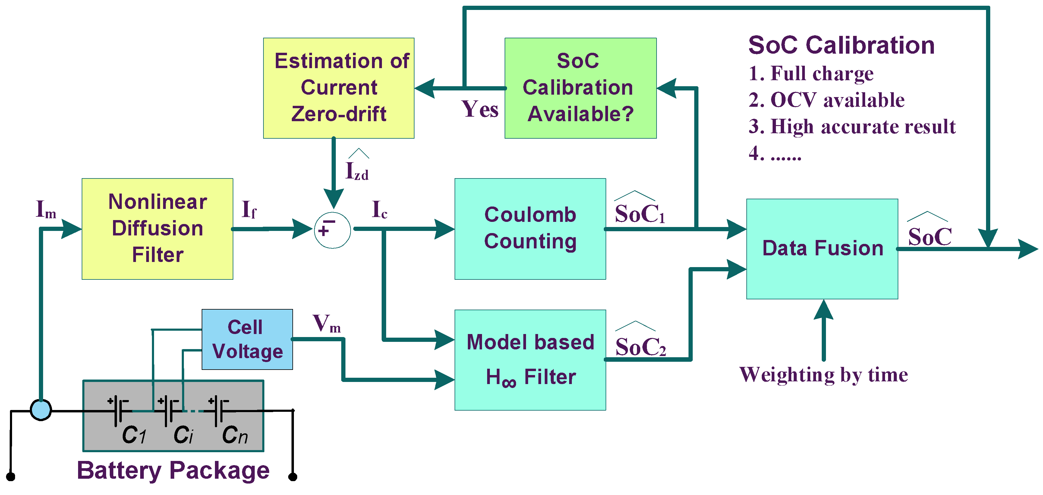
Therefore, to guarantee the estimation accuracy in real driving process, it is necessary to improve anti-noise and self-adaptive abilities, i.e., the robustness, of SoC estimation techniques. In this paper, we have proposed a robust estimation framework, as shown in Figure 1, which consists of:

• A nonlinear diffusion filter to remove current measurement noise, where $I_m$ is the measured current and $I_f$ is the filtering result.
• A current zero-drift estimator to reduce the zero-drift, where $\widehat{I_{zd}}$ is the estimated zero-drift of current measurement and $I_c=I_f-\widehat{I_{zd}}$ is the “clean” result.
• A coulomb counting estimator to implement open-loop estimation $\widehat{So{C}_1}$.
• A H${}_{\infty }$ filter to realize robust closed-loop estimation under model uncertainty and inaccuracy, where $V_m$ is the measured terminal voltage and $\widehat{So{C}_2}$ is the estimated SoC.
• A data fusion component to achieve the final estimation $\widehat{SoC}$ by balancing $\widehat{So{C}_1}$ and $\widehat{So{C}_2}$.

Section 2 firstly analyzes the quasi-random property of battery current in driving process, and then applies nonlinear diffusion filter to achieve better noise reduction performance than linear digital filter and wavelet based filter. In Section 3, based on the estimation error of coulomb counting method obtained at each SoC calibration available time, a self-learning strategy is proposed to estimate the zero-drift of current measurement. In Section 4, we introduce $H_{\infty }$ filter to robustly estimate SoC and conduct simulations to compare performance with conventional EKF. In Section 5, a data fusion unit is designed to obtain the final SoC value and the overall estimation framework has been demonstrated in simulation. Conclusions and future works are given in Section 6.

Figure 1. The proposed robust SoC estimation framework.

Figure 1. The proposed robust SoC estimation framework.

2. Current Denoising Using Nonlinear Diffusion Filter

Battery is a typical less-information system, where complex multi-parameter electrochemical reaction occurs inside, while only terminal voltage, bus current and surface temperature can be measured outside. SoC, one of the internal states, has to be estimated according to the limited external variables. Thus, the measurement accuracies of these variables are crucial for SoC estimation.

2.1. Property Analysis of Current Measurement

A power battery package usually consists of tens of, even hundreds of, series/paralle connected cells to generate large charge/discharge current varying in ±300A [33]. However the precision of commercialized current sensors is around $\pm 1\%$, resulting a maximum error of $\pm 3A$. The error is non-ignorable for SoC estimation. Moreover, although the peak current can reach 300A, the current in most time is less than 100A, thus the $\pm 3A$ noise becomes comparatively larger in percentage.

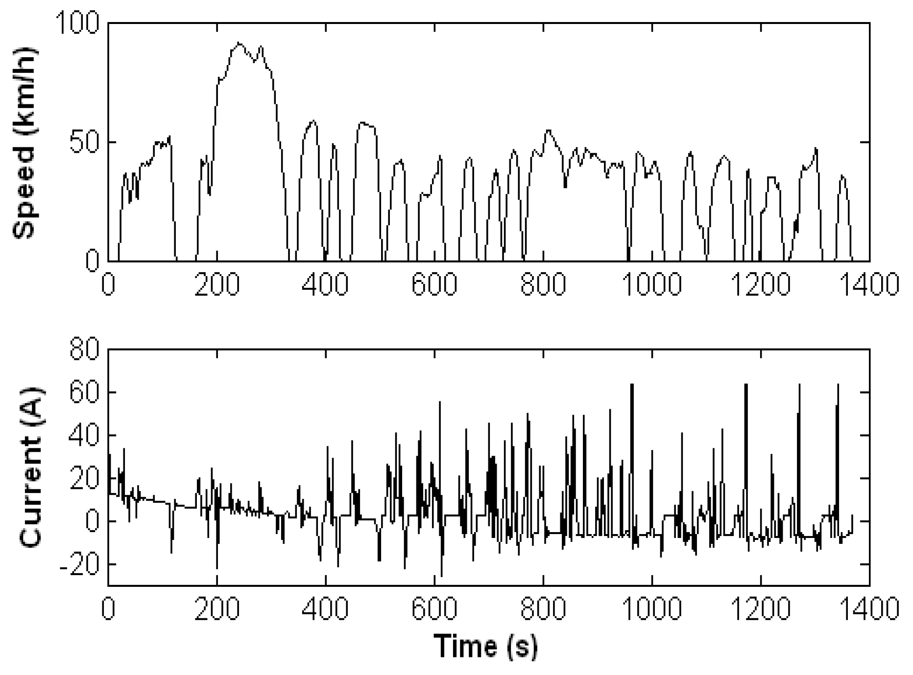
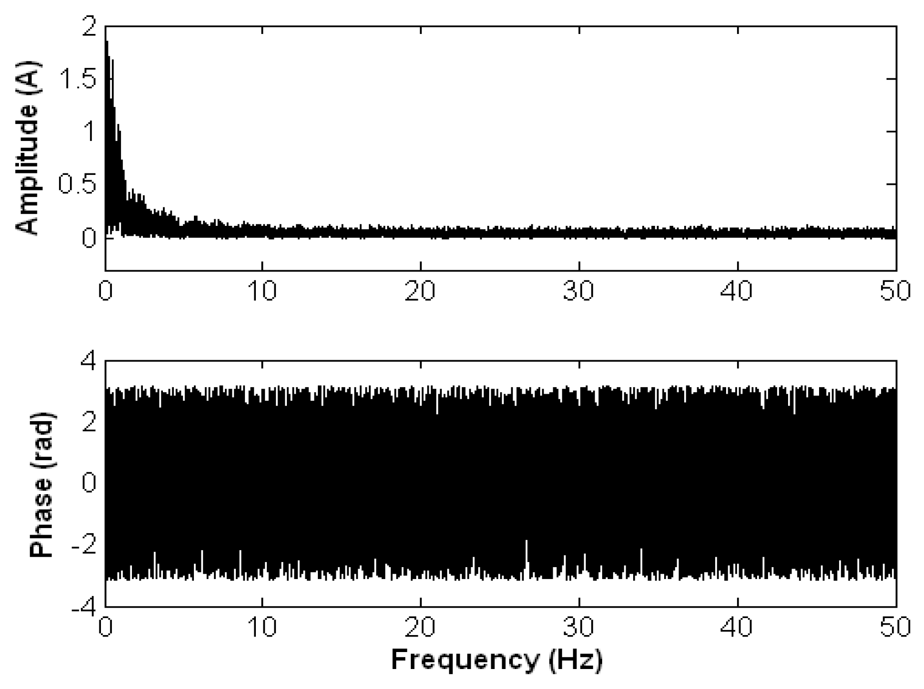
Another distinct difficulty is that the signal possesses quasi-random property, which leads to the failure of traditional filters. Figure 2 illustrates a typical current profile of Prius driving on cycle UDDS, which is simulated by Advisor [34]. Battery current is determined by the demands of motor and/or generator, which primarily depend on the driving behaviors. Since how to drive a vehicle is limited by road conditions and usually disturbed by various unexpected events, such as crawl by traffic jam, scram to avoid pedestrians crossing the street, sudden acceleration for overtaking and so forth, the erratic driving will definitely result in quasi-random current on power bus. Analysis in frequency domain further depicts the property of battery current, as shown in Figure 3. The current signal, with 100 Hz sampling frequency, expands in the whole frequency domain and is hard to determine a cut-off frequency which separates signal from noise.

Figure 2. Current profile of Prius driving on cycle UDDS.

Figure 2. Current profile of Prius driving on cycle UDDS.

Figure 3. Frequency analysis of current profile of Prius driving on cycle UDDS.

Figure 3. Frequency analysis of current profile of Prius driving on cycle UDDS.

Noise reduction essentially requires the property difference between signal and noise in some way. As discussed above, the similar frequency property between current signal and noise causes the difficulty in applying traditional filters, e.g., low-pass filter, to isolate noise.

The variation of real current signal is caused by driving behaviors, which usually leads to a comparative large degree of change. However the current noise is often produced by the precisions of measurement units, electromagnetic interference, vehicle vibrations and so on, which typically varies in a small range. Therefore, based on the degree of change, i.e., the difference, we apply the nonlinear diffusion filter to reduce noise.

2.2. Nonlinear Diffusion Filter

Nonlinear Diffusion Filter (NDF) was firstly proposed in image processing field to nonlinearly eliminate the oscillation in small range while keep the variation in large scale [35].

Denoting k and i as the discrete time and iteration index, the iterative equation of nonlinear diffusion filter is described as

$$\begin{array}{c}I(k,i+1)=I(k,i)+\Delta t\times c_l(k,i)\times \left[I(k-1,i)-I(k,i)\right]\hfill \\ +\Delta t\times c_r(k,i)\times \left[I(k+1,i)-I(k,i)\right]\hfill \end{array}$$

(1)

where initial iteration $I(k,1)$ is set as the measured data sequence $I_m\left(k\right)$, the last iteration $I(k,N)$ is the filtering result $I_f\left(k\right)$, and N is the iteration time.

As iterative step, a large $\Delta t$ stands for a long diffusion period in each iteration, leading to smoother results, however, with the risk of unstable iteration process. In contrast, too small $\Delta t$ causes a slow diffusion process, requiring more iterations to achieve a satisfactory result.

$c_l(k,i)$ and $c_r(k,i)$, generally denoted by $c(k,i)$, are the left and right diffusion coefficients respectively, which control the degree to smooth the values between the kth datum and its left or right neighbor. The smaller $c(k,i)$ is, the harder to smooth. As discussed above, a large change of current has high possibility to be real signal while a small one usually suffers from noise. Thus, we set $c(k,i)$ inversely proportioned to the signal difference, using the conventional equation:

$$c_l(k,i)=\frac{1}{1+{\left[\frac{I(k-1,i)-I(k,i)}{\kappa }\right]}^2}$$

(2)

and

$$c_r(k,i)=\frac{1}{1+{\left[\frac{I(k+1,i)-I(k,i)}{\kappa }\right]}^2}$$

(3)

where κ is gradient modulus threshold that controls the conduction.

2.3. Adaptive-κ Strategy

Equations (2) and (3) indicate that the performance of nonlinear diffusion filter depends on the selection of κ. In general, a noisy signal with low Signal-Noise-Ratio (SNR) requires a large κ to enhance the smoothing effect. However, the SNR of noisy signal is an unknown value and has to be estimated indirectly. Based on the character of battery current, an adaptive κ selection method is proposed as the following steps.

• Calculate the differential signal $\Delta I_m\left(k\right)$ of the original signal $I_m\left(k\right)$.

  $$\Delta I_m\left(k\right)=I_m(k+1)-I_m\left(k\right)$$

  (4)
• Establish the set ${\Delta }_s$ in which the absolute values of differential signal are smaller than 5A. The reason to remove higher differential data is that they are likely caused by driving behavior, i.e., the real current change.

  $${\Delta }_s=\{\Delta I_m\left(k\right)\mid |\Delta I_m\left(k\right)|<5\}$$

  (5)
• Calculate the standard deviation $std\left({\Delta }_s\right)$ of the elements in set ${\Delta }_s$. To some extent, $std\left({\Delta }_s\right)$ is an indicator of the SNR of signal. The smaller $std\left({\Delta }_s\right)$ is, the larger SNR is.
• Adaptively determine κ according to $std\left({\Delta }_s\right)$. In this study, we first fix the iteration time $N=20\times f_s$ ($f_s$ stands for sampling frequency) and the iterative step $\Delta t=0.6$, then the relationship between κ and $std\left({\Delta }_s\right)$ is experimentally determined by the below piecewise function.

  $$\kappa =\left\{\begin{array}{c}min(std\left({\Delta }_s\right)/10,2)std\left({\Delta }_s\right)>2.2\hfill \\ max(std\left({\Delta }_s\right)\times 1.76-3.652,0)std\left({\Delta }_s\right)<2.2\hfill \end{array}\right.$$

  (6)

Remark: As nonlinear diffusion filter requires the right neighbors (future data) to smooth the current datum, the filter has to delay for a percoid. In this work, the iteration time $N=20\times f_s$ will result in 20 seconds delay, which is small enough to be negligible because SoC changes slowly.

2.4. Performance Comparison

To demonstrate the efficacy of nonlinear diffusion filter with adaptive-κ, performance comparison with the traditional lowpass filter and wavelet filter are conducted. The lowpass filter is implemented by Butterworth method with trial-and-error determined cutoff frequency $f_{cut}=0.9\times (f_s/2)$ and the wavelet filter uses level-dependent thresholds determined by Birge-Massart strategy [36].

The real current profiles are produced by Advisor. We select the well-developed “Prius_jpn” vehicle model and three typical driving cycles: the highway “HWFET”, the suburban “WVUSUB”, and the urban “MANHATTAN”. The real current is corrupted by white noises with SNR from 0dB to 20dB.

The performance index Reduced Root-Mean-Square of Errors (RRMSoE) is defined as below.

$$RRMSoE\left[A\right]=rms(I,I_m)-rms(I,I_f)$$

(7)

and

$$RRMSoE[\%]=\frac{rms(I,I_m)-rms(I,I_f)}{rms(I,I_m)}\times 100\%$$

(8)

where

$$rms(I_1,I_2)=\sqrt{\frac{1}{L}{\displaystyle \sum _{i=1}^L}{(I_1\left(i\right)-I_2\left(i\right))}^2}$$

(9)

I, $I_m$ and $I_f$ are the real current, measured noisy current and filtering result respectively, L is the length of data.

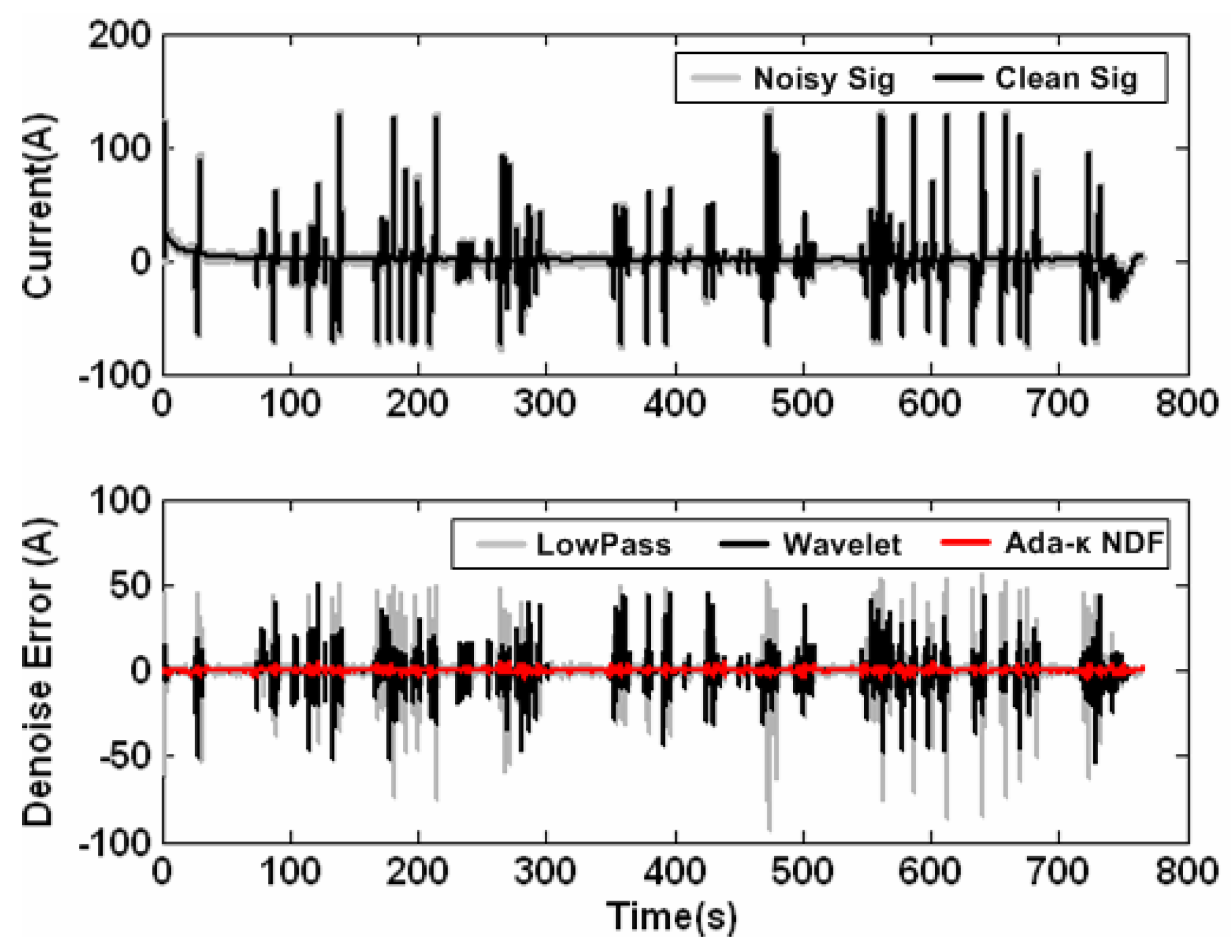
As an example, Figure 4 illustrates the HWFET case with 15dB SNR noise. The top subfigure describes the real current signal and the noisy signal. It is clear that the real signal dominates the large variance. Added noises appear as burrs. The errors of filtering results are given in the bottom subfigure. Without a doubt, the lowpass filter gives poor performance, even worse than noisy signal, because it simultaneously removes the real signal in high frequency zone. Basically, any frequency based filter is difficult to handle this problem. Wavelet filter, focusing on both scale and time aspects, has better results than lowpass filter but still fails to keep the large variation of real signal. The nonlinear diffusion filter successfully removes the noise appearing as burrs while keeps the real signal which possesses large variation in morphology.

Figure 4. Filtering results of HWFET current profile corrupted by noise with 15dB SNR.

Figure 4. Filtering results of HWFET current profile corrupted by noise with 15dB SNR.

The total results are given in Table 1, where each value is the average of 100 independent random tests. It is clear that the adaptive-κ strategy efficiently estimates the equivalent SNR in each case and hence calculates a suitable κ to achieve satisfactory denoising.

Table 1. Reduced RMS of denoising errors based on different filters.

SNR [dB]	Highway(HWFET)						Suburban(WVUSUB)						Urban(MANHATTAN)
	Lowpass		Wavelet		Ada-κ NDF		Lowpass		Wavelet		Ada-κ NDF		Lowpass		Wavelet		Ada-κ NDF
	[A]	[%]	[A]	[%]	[A]	[%]	[A]	[%]	[A]	[%]	[A]	[%]	[A]	[%]	[A]	[%]	[A]	[%]
0	-2.05	-21.98	2.98	31.95	5.53	59.41	0.00	-0.04	4.82	52.09	6.68	72.15	-0.14	-1.22	5.57	49.58	6.76	60.23
2	-2.62	-35.47	1.57	21.26	4.11	55.53	-0.24	-3.29	3.85	52.35	5.33	72.53	-0.43	-4.83	4.33	48.50	5.77	64.69
4	-3.14	-53.41	0.41	7.02	2.82	47.93	-0.44	-7.58	3.07	52.52	4.04	69.25	-0.70	-9.85	3.27	46.15	4.32	60.94
6	-3.77	-80.85	-0.58	-12.34	1.86	39.84	-0.67	-14.52	2.42	52.15	2.99	64.44	-0.99	-17.66	2.35	41.75	3.10	55.14
8	-4.24	-114.45	-1.42	-38.27	1.08	29.03	-0.91	-24.73	1.88	51.01	2.18	59.30	-1.33	-29.67	1.53	34.28	2.11	47.13
10	-4.73	-160.50	-2.11	-71.68	0.71	24.00	-1.16	-39.61	1.44	49.30	1.58	54.08	-1.63	-45.89	0.86	24.24	1.44	40.53
12	-5.16	-220.51	-2.67	-114.30	0.70	29.84	-1.40	-60.15	1.06	45.47	1.29	55.32	-1.96	-69.49	0.28	10.00	1.06	37.72
14	-5.51	-296.75	-3.12	-168.11	0.94	50.74	-1.63	-88.11	0.72	39.25	1.20	64.90	-2.24	-100.18	-0.21	-9.19	0.93	41.54
16	-5.81	-393.55	-3.49	-236.44	0.80	54.51	-1.84	-125.45	0.43	29.53	0.93	63.17	-2.52	-141.40	-0.63	-35.24	1.00	56.34
18	-6.07	-517.99	-3.78	-322.74	0.63	53.77	-2.03	-174.06	0.18	15.67	0.73	62.35	-2.76	-195.17	-0.96	-67.62	0.76	53.99
20	-6.28	-674.39	-4.02	-431.19	0.49	52.57	-2.20	-237.73	-0.02	-2.45	0.57	62.03	-2.96	-263.57	-1.23	-109.44	0.59	52.19

Table 1. Reduced RMS of denoising errors based on different filters.

SNR [dB]	Highway(HWFET)						Suburban(WVUSUB)						Urban(MANHATTAN)
	Lowpass		Wavelet		Ada-κ NDF		Lowpass		Wavelet		Ada-κ NDF		Lowpass		Wavelet		Ada-κ NDF
	[A]	[%]	[A]	[%]	[A]	[%]	[A]	[%]	[A]	[%]	[A]	[%]	[A]	[%]	[A]	[%]	[A]	[%]
0	-2.05	-21.98	2.98	31.95	5.53	59.41	0.00	-0.04	4.82	52.09	6.68	72.15	-0.14	-1.22	5.57	49.58	6.76	60.23
2	-2.62	-35.47	1.57	21.26	4.11	55.53	-0.24	-3.29	3.85	52.35	5.33	72.53	-0.43	-4.83	4.33	48.50	5.77	64.69
4	-3.14	-53.41	0.41	7.02	2.82	47.93	-0.44	-7.58	3.07	52.52	4.04	69.25	-0.70	-9.85	3.27	46.15	4.32	60.94
6	-3.77	-80.85	-0.58	-12.34	1.86	39.84	-0.67	-14.52	2.42	52.15	2.99	64.44	-0.99	-17.66	2.35	41.75	3.10	55.14
8	-4.24	-114.45	-1.42	-38.27	1.08	29.03	-0.91	-24.73	1.88	51.01	2.18	59.30	-1.33	-29.67	1.53	34.28	2.11	47.13
10	-4.73	-160.50	-2.11	-71.68	0.71	24.00	-1.16	-39.61	1.44	49.30	1.58	54.08	-1.63	-45.89	0.86	24.24	1.44	40.53
12	-5.16	-220.51	-2.67	-114.30	0.70	29.84	-1.40	-60.15	1.06	45.47	1.29	55.32	-1.96	-69.49	0.28	10.00	1.06	37.72
14	-5.51	-296.75	-3.12	-168.11	0.94	50.74	-1.63	-88.11	0.72	39.25	1.20	64.90	-2.24	-100.18	-0.21	-9.19	0.93	41.54
16	-5.81	-393.55	-3.49	-236.44	0.80	54.51	-1.84	-125.45	0.43	29.53	0.93	63.17	-2.52	-141.40	-0.63	-35.24	1.00	56.34
18	-6.07	-517.99	-3.78	-322.74	0.63	53.77	-2.03	-174.06	0.18	15.67	0.73	62.35	-2.76	-195.17	-0.96	-67.62	0.76	53.99
20	-6.28	-674.39	-4.02	-431.19	0.49	52.57	-2.20	-237.73	-0.02	-2.45	0.57	62.03	-2.96	-263.57	-1.23	-109.44	0.59	52.19

3. Self-learning Strategy for Current Zero-Drift Reduction

Although the nonlinear diffusion filter has the ability to remove the oscillatory noise, it can not handle the zero-drift problem which causes the baseline shift. Zero-drift, actually the non-zero mean of noise, is the source making coulomb counting obtain divergent result and negatively affecting the performances of other estimators.

In this section, we propose a self-learning strategy to estimate the zero-drift of current measurement. To establish the self-learning system, it is necessary to know the estimation error, equally the real SoC. In practice, the truth value of SoC can be obtained when (1) battery is full charged, (2) OCV is available or (3) higher accurate result is obtained somehow. In these calibration-available moments, we can not only reset the SoC estimation but also calculate the zero-drift using the error of coulomb counting, as deduced in the following.

The discrete recursive equation of coulomb counting is described as

$$\widehat{So{C}_1}\left(k\right)=\widehat{So{C}_1}(k-1)+\frac{I_c\left(k\right)\eta \left(k\right)T_s}{Q_{full}}$$

(10)

where $\widehat{So{C}_1}\left(k\right)$ is the estimated SoC at time k, $I_c\left(k\right)$ is the “clean” current, $Q_{full}$ is the charge stored in the full-charged battery, and $T_s$ is the sampling period. $\widehat{So{C}_1}\left(0\right)$ is initialized by SoC-OCV mapping table or other advanced methods at each start time or reset to true value at each calibration-available time.

$\eta \left(k\right)$ is the coulombic efficiency or ampere-hour efficiency. Strictly speaking, it is a time-variant parameter, depending on temperature, SoC and other relative states. The basic way to determine coulombic efficiency is establishing its value table according to the manufacturers’ datasheets or testing data [37]. The mass utilization of coulomb counting in practical application has demonstrated its feasibility and validity. In addition, adaptive learning and on-line estimation strategies can strengthen the accuracy of coulombic efficiency estimation [6,7,29]. Moreover, since the accuracy of the coulomb counting primarily depends on measurement of the battery current and estimation of the initial SoC [7], the error of coulombic efficiency will be neglected in this paper.

To analyze the zero-drift of current measurement, we denote the truth value of current as $I\left(k\right)$, the residual noise affecting coulomb counting estimator as $I_n\left(k\right)$, and the truth value of SoC as $SoC\left(k\right)$. The “clean” current accumulated in coulomb counting method actually is expressed by

$$I_c\left(k\right)=I\left(k\right)+I_n\left(k\right)$$

(11)

and

$$\begin{array}{c}\widehat{So{C}_1}\left(k\right)=\widehat{So{C}_1}(k-1)+\frac{I_c\left(k\right)\eta \left(k\right)T_s}{Q_{full}}\hfill \\ =\widehat{So{C}_1}\left(0\right)+\frac{{\displaystyle \sum _{i=0}^k}{I}_c\left(k\right)\eta \left(i\right)T_s}{Q_{full}}\hfill \\ =\widehat{So{C}_1}\left(0\right)+\frac{T_s\left({\displaystyle \sum _{i=0}^k}I\left(i\right)\eta \left(i\right)+{\displaystyle \sum _{i=0}^k}{I}_n\left(i\right)\eta \left(i\right)\right)}{Q_{full}}\hfill \\ =\left(\widehat{So{C}_1}\left(0\right)+\frac{T_s{\displaystyle \sum _{i=0}^k}I\left(i\right)\eta \left(i\right)}{Q_{full}}\right)+\frac{T_s{\displaystyle \sum _{i=0}^k}{I}_n\left(i\right)\eta \left(i\right)}{Q_{full}}\hfill \end{array}$$

(12)

Since $\widehat{So{C}_1}\left(0\right)$ is initialized at each start time by SoC-OCV mapping table or advanced algorithms or is reset to “true” value at each calibration-available moment, its error is small enough to be neglected in tolerance range. Therefore we have

$$\widehat{So{C}_1}\left(0\right)=SoC\left(0\right)$$

(13)

$$\widehat{So{C}_1}\left(k\right)=SoC\left(k\right)+\frac{T_s{\displaystyle \sum _{i=0}^k}{I}_n\left(i\right)\eta \left(i\right)}{Q_{full}}$$

(14)

$$E\left(\widehat{So{C}_1}\left(k\right)-SoC\left(k\right)\right)=E\left(\frac{T_s{\displaystyle \sum _{i=0}^k}{I}_n\left(i\right)\eta \left(i\right)}{Q_{full}}\right)=\frac{T_s{\displaystyle \sum _{i=0}^k}\eta \left(i\right)}{Q_{full}}E\left(I_n\left(i\right)\right)$$

(15)

At each calibration-available time $k^{*}$, the truth value $SoC\left(k^{*}\right)$ is available, thus

$$\widehat{So{C}_1}\left(k^{*}\right)-SoC\left(k^{*}\right)=\frac{T_s{\displaystyle \sum _{i=0}^{k^{*}}}\eta \left(i\right)}{Q_{full}}E\left(I_n\left(i\right)\right)$$

(16)

The zero-drift of current measurement $\widehat{I_{zd}}$ actually is the mean of noise:

$$\widehat{I_{zd}}=E\left\{I_n\left(i\right)\right\}=\frac{Q_{full}\left[\widehat{So{C}_1}\left(k^{*}\right)-SoC\left(k^{*}\right)\right]}{T_s{\displaystyle \sum _{i=0}^{k^{*}}}\eta \left(i\right)}$$

(17)

At each calibration available moment, $\widehat{I_{zd}}$ is updated by Equation (17), which enables online tracking of zero-drift.

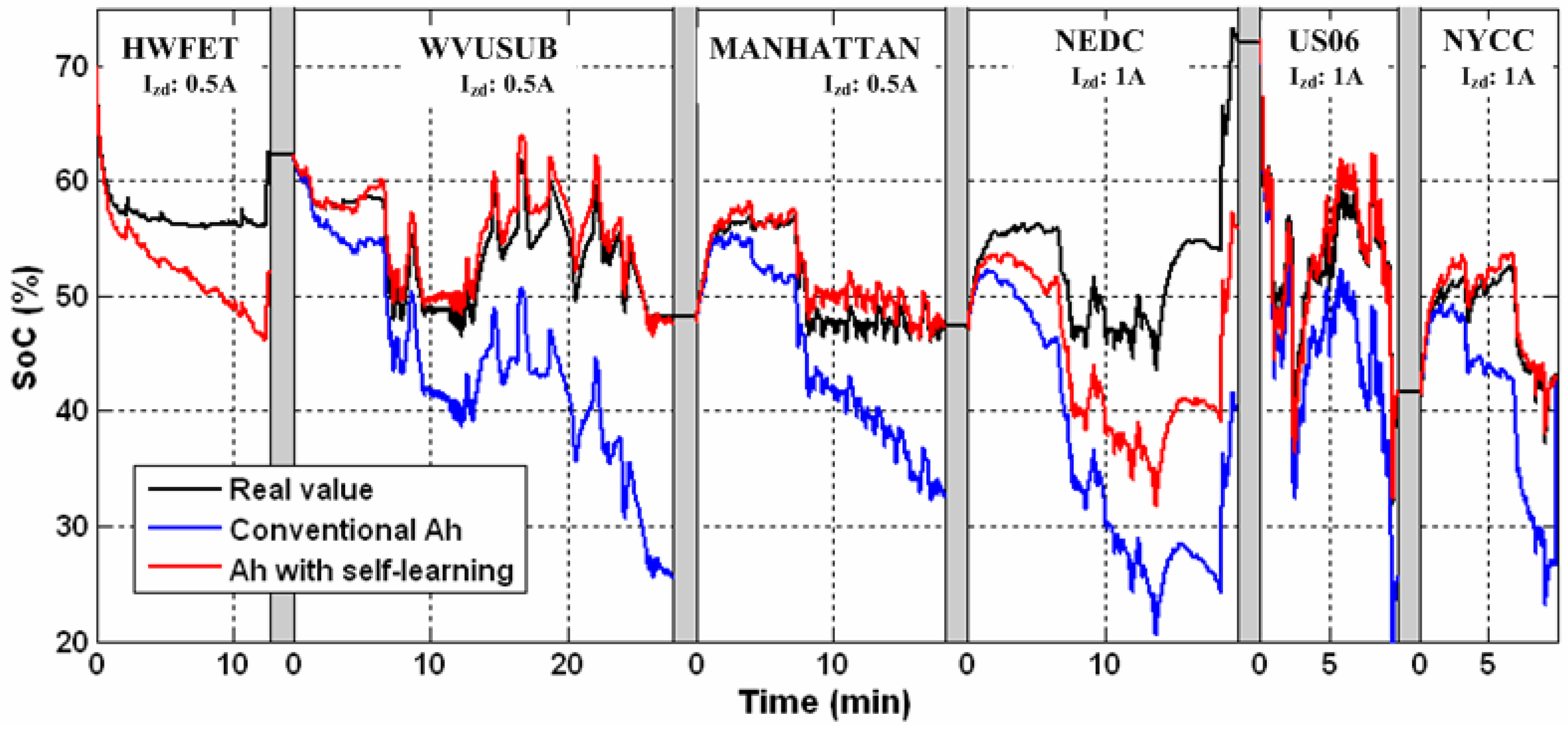
To demonstrate the availability and efficacy, a simulation based on Advisor has been conducted to track SoC of Prius driving successively on the cycles HWFET, WVUSUB, MANHATTAN, NEDC, US06, and NYCC. After completion of each cycle, a half-hour stop allows the battery OCV available. When vehicle starts the new driving cycle, BMS will reset SoC to real value and re-estimate zero-drift. The SNR of current measurement is set to 0dB. The zero-drift $I_{zd}$ is set to 0.5A in the 1st-3rd cycles and 1A in the 4th-6th cycles. BMS firstly denoises the current by ada-κ NDF and then removes the zero-drift by subtracting estimation value $\widehat{I_{zd}}$.

Figure 5 shows the SoC tracking results comparing the performances using or not using zero-drift self-learning strategy and Table 2 summarizes the numerical indexes of each cycle, including the average (ave) of absolute SoC estimation errors and the standard deviation (std) of errors in each cycle. In the first driving cycle HWFET, since we have no prior knowledge about zero-drift, its estimation value is set to 0 and therefore reaches the same SoC tracking performance with conventional method. In the following two cycles, OCV is available at each start time to calibrate SoC and calculate estimation error of the previous cycle, which allows the update of $\widehat{I_{zd}}$. The estimation values of zero-drift are 0.4895 A and 0.4952 A respectively, which are very close to real zero-drift 0.5 A. Thus, the estimation error of proposed method is obviously smaller than conventional algorithm. In the 4th cycle, the real zero-drift is changed to 1A, aiming at testing the self-adaptive ability of learning strategy. As the learning strategy determines zero-drift by using the error in last cycle, the one cycle delay causes that $\widehat{I_{zd}}=0.4987$ can not fully compensate the real 1A drift and results nonconvergent SoC estimation. In the following cycles, the large error updates the $\widehat{I_{zd}}$ to be 0.9863 and 0.9967 in 5th and 6th cycles respectively. The self-adaptive ability leads to satisfactory performance in the last two cycles.

Table 2. Numerical results of SoC tracking using or not using self-learning strategy (unit [%]).

SoC estimation methods	HWFET		WVUSUB		MANHATTAN		NEDC		US06		NYCC
	ave	std	ave	std	ave	std	ave	std	ave	std	ave	std
Conventional Ah	4.71	2.71	9.87	6.22	6.20	4.04	16.21	9.36	7.74	4.36	7.16	4.86
Ah with self-learning	4.71	2.71	1.34	0.96	1.23	0.95	8.24	4.77	1.42	1.65	0.96	0.50

Table 2. Numerical results of SoC tracking using or not using self-learning strategy (unit [%]).

SoC estimation methods	HWFET		WVUSUB		MANHATTAN		NEDC		US06		NYCC
	ave	std	ave	std	ave	std	ave	std	ave	std	ave	std
Conventional Ah	4.71	2.71	9.87	6.22	6.20	4.04	16.21	9.36	7.74	4.36	7.16	4.86
Ah with self-learning	4.71	2.71	1.34	0.96	1.23	0.95	8.24	4.77	1.42	1.65	0.96	0.50

Figure 5. SoC estimation results based on conventional coulomb counting and the proposed coulomb counting with self-learning strategy (white noise with 0dB SNR, zero-drift 0.5A for the 1st-3rd cycles and 1A for the 4th-6th cycles). The gray bars between cycles represent half-hour stops which allow OCV available.

Figure 5. SoC estimation results based on conventional coulomb counting and the proposed coulomb counting with self-learning strategy (white noise with 0dB SNR, zero-drift 0.5A for the 1st-3rd cycles and 1A for the 4th-6th cycles). The gray bars between cycles represent half-hour stops which allow OCV available.

Although the proposed framework significantly improves the performance of conventional coulomb counting method, it inherently is an open loop estimator which does not take the measurable voltage into consideration. It only self-corrects estimation results at calibration moments but can not revise the errors during driving process. Therefore, in the following sections, we introduce H${}_{\infty }$ filter to establish closed-loop estimation of SoC and apply a data fusion unit to determine the final SoC value.

4. Robust SoC Estimation using H${}_{\infty }$ Filter

Battery is a typical time-variant system, with tight relation to ambient temperature, life age, and SoC. Online identification is the popular strategy to solve time-variant problem, however, at the cost of high time consumption and inaccurate identification result due to noises. An alternative way is robust estimation technique, which constructs a suboptimal filter with the ability to minimize the maximum estimation error caused by noises and uncertainties of system model.

In pace with the development of H${}_{\infty }$ control theory, researchers have shown great interest in H${}_{\infty }$ filter [38,39]. A good introduction and review can be found in [40]. In contrary to Kalman filter, H${}_{\infty }$ filter is proposed to handle estimation problems under uncertain model structure, model parameters and system noises. It has two main features: (1) do not require any assumptions of the disturbances and model uncertainties; (2) minimize the estimation error in the worst situation. Therefore, it is more applicable than Kalman filter in practical application.

4.1. H${}_{\infty }$ Filter Algorithm

Denoting x as the system state vector, y the output vector, u the input vector, w the process noise, and v the measurement noise, a system state space equations are expressed as:

$$\begin{array}{c}{x}_{k+1}=A_k{x}_k+B_k{u}_k+{\Gamma }_k{w}_k\hfill \\ y_k=C_k{x}_k+D_k{u}_k+v_k\hfill \end{array}$$

(18)

The suboptimal H${}_{\infty }$ filtering problem is formalized as: given estimation error bounder $\gamma >0$, find an estimation of ${\widehat{z}}_k=F_f(u_0,\cdots ,u_k,y_0,\cdots ,y_k)$ such that

$$\underset{F_f}{inf}\underset{x_0,w\in H_2,v\in H_2}{sup}\frac{{∥z_k-{\widehat{z}}_k∥}_2^2}{{∥x_0-{\widehat{x}}_0∥}_{P_0^{-1}}^2+{∥w_k∥}_2^2+{∥v_k∥}_2^2}<{\gamma }^2$$

(19)

where $z_k=L_k{x}_k$ is the estimation goal, i.e., the linear combination of system states, $L_k$ is user-defined state weight matrix, and ${∥{\chi }_k∥}_2^2={\sum }_{i=0}^k{\chi }_i^{*}{\chi }_i$ .

The solution of the suboptimal $H_{\infty }$ filtering problem can be calculated by the following recursion formulas:

$${\widehat{x}}_{k+1,k}=A_k{\widehat{x}}_k+B_k{u}_k$$

(20)

$$R_k=\left[\begin{array}{cc}I& 0\\ 0& -{\gamma }^{2}I\end{array}\right]+\left[\begin{array}{c}{C}_k\\ L_k\end{array}\right]P_k\left[\begin{array}{cc}{C}_k^T& L_k^T\end{array}\right]$$

(21)

$$P_{k+1}=A_k{P}_k{A}_k^T+{\Gamma }_k{\Gamma }_k^T-A_k{P}_k\left[C_k^T{L}_k^T\right]R_k^{-1}\left[\begin{array}{c}{C}_k\\ L_k\end{array}\right]P_k{A}_k^T$$

(22)

$$K_{k+1}=P_{k+1}{C}_{k+1}^T{\left[I+C_{k+1}{P}_{k+1}{C}_{k+1}^T\right]}^{{}_{-1}}$$

(23)

$${\widehat{x}}_{k+1}={\widehat{x}}_{k+1,k}+K_{k+1}(y_{k+1}-C_{k+1}{\widehat{x}}_{k+1,k}-D_{k+1}{u}_{k+1})$$

(24)

$${\widehat{z}}_{k+1}=L_{k+1}{\widehat{x}}_{k+1}$$

(25)

under the conditions that $[A_k$ ${\Gamma }_k]$ has full rank and

$$P_k^{-1}+C_k^T{C}_k-{\gamma }^{-2}{L}_k^T{L}_k>0forallk$$

(26)

¿From the above formulas, it is clear that if $L\left(k\right)=I$ and $\gamma \to \infty$, $H_{\infty }$ filter degrades to be Kalman filter. Thus, Kalman filter is a special situation of $H_{\infty }$ filter with infinite $H_{\infty }$ norm, and hence results in the worse robustness.

4.2. Battery Modeling

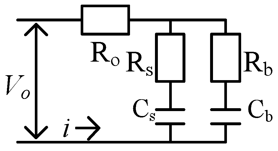
As shown in Figure 6, we apply battery RC equivalent circuit model in this paper [10]. The RC model consists of a bulk capacitor $C_b$ and a surface capacitor $C_s$, which simulate energy storage and dynamic property of the battery respectively. Output resistance $R_o$, surface resistance $R_s$ and bulk resistance $R_b$ are used to model the internal resistance of battery.

By selecting state vector as the voltages of bulk and surface capacitors $x_k={[V_{bk},V_{sk}]}^{\prime }$, system input as bus current $u_k=I_k$, output as terminal voltage $y_k=V_{ok}$, and sampling time as $T_s$, the discrete state space Equation (18) are concrete into the following matrixes.

$$A=\left[\begin{array}{cc}1-\frac{T_s}{C_b(R_b+R_s)}& \frac{T_s}{C_b(R_b+R_s)}\\ \frac{T_s}{C_s(R_b+R_s)}& 1-\frac{T_s}{C_s(R_b+R_s)}\end{array}\right]$$

(27)

$$B=\left[\begin{array}{c}\frac{-R_s{T}_s}{C_b(R_b+R_s)}\\ \frac{-R_b{T}_s}{C_s(R_b+R_s)}\end{array}\right]$$

(28)

$$C=\left[\begin{array}{cc}\frac{R_s}{R_b+R_s}& \frac{R_b}{R_b+R_s}\end{array}\right]$$

(29)

$$D=-R_o-\frac{R_b{R}_s}{R_b+R_s}$$

(30)

The SoC for the RC model was estimated by using the voltages of the two capacitors. Since $C_b$ represents the bulk energy in the battery, it contributes the majority of SoC, as expressed in the below equations.

$$\widehat{So{C}_2}\left(k\right)=\frac{1}{21}\left[20\widehat{So{C}_{C_b}}\left(k\right)+\widehat{So{C}_{C_s}}\left(k\right)\right]$$

(31)

where

$$\widehat{So{C}_{C_b}}\left(k\right)=F_{OCV-SoC}\left(V_{bk}\right)=F_{OCV-SoC}\left(x_k\left(1\right)\right)$$

(32)

$$\widehat{So{C}_{C_s}}\left(k\right)=F_{OCV-SoC}\left(V_{sk}\right)=F_{OCV-SoC}\left(x_k\left(2\right)\right)$$

(33)

and $F_{OCV-SoC}(·)$ is the function mapping OCV to SoC. It usually is predetermined by manufactory’s datasheet or experimental testing data.

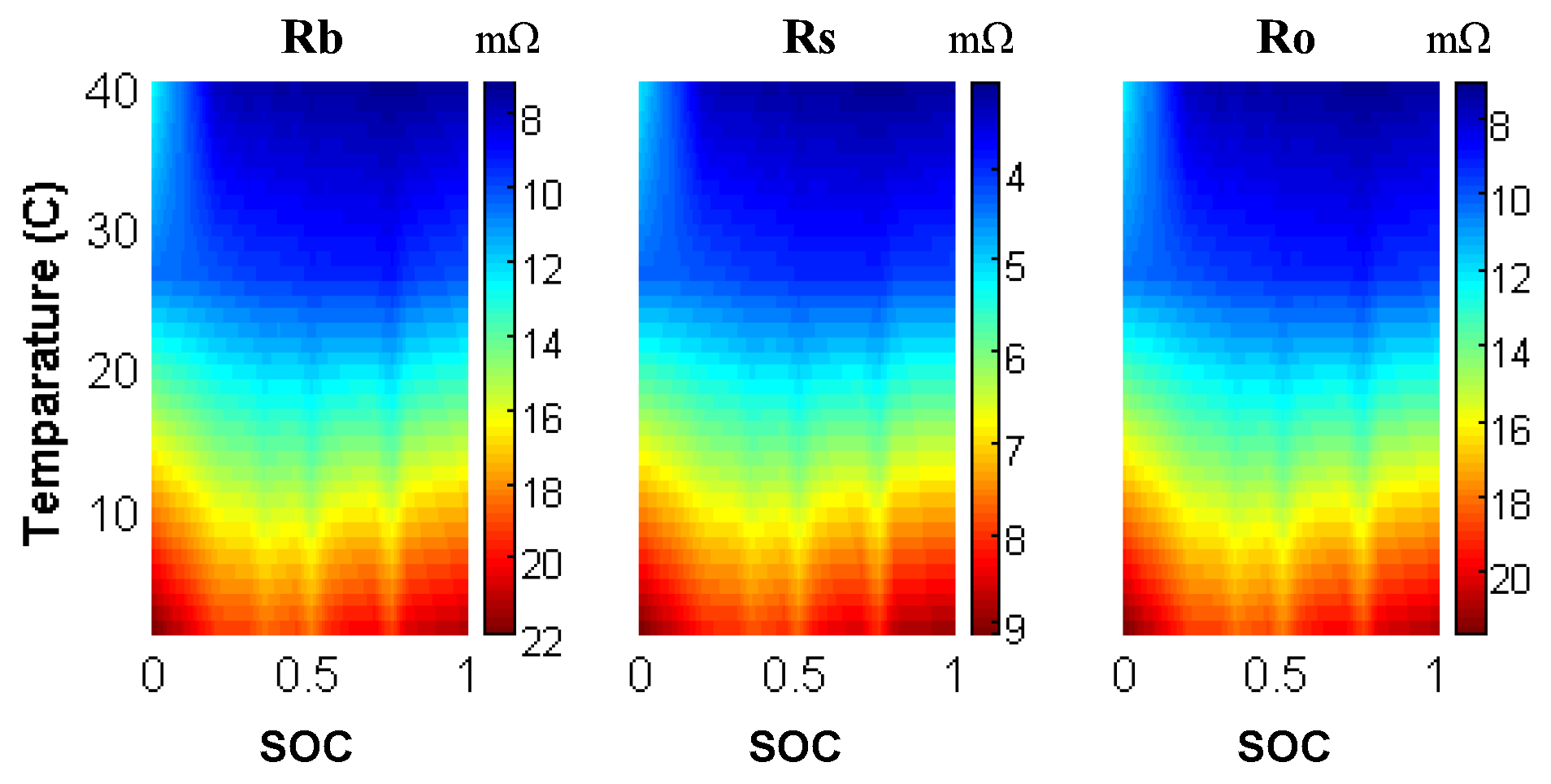
Figure 6. Battery RC Model.

Figure 6. Battery RC Model.

Model parameters essentially will change in the running process. A kind of 6.5 Ah Prismatic Panasonic NiMH Battery has been tested at NREL Battery Thermal Management Lab and corresponding model parameters are provided by Advisor [34]. Figure 7 shows the change in resistances of resistors versus temperature and SoC. Taking the output resistor as an example, it is clear that the maximum resistance is $0.0216\Omega$, more than 3 times of the minimum value $0.0071\Omega$. The significant variation of model parameters is worthy of paying special attention in the design of SoC estimator. Other resistors and capacitors have the similar properties.

Figure 7. Resistance variance of resistors in RC model.

Figure 7. Resistance variance of resistors in RC model.

Since the model error is hard to determine aforehand, we leave this difficulty to H${}_{\infty }$ filter and estimate Γ only according to current noise. The measured current $u=I_c=I+I_n$, where I is the clean signal and $I_n$ is the current noise. Therefore, $Bu=BI+B{I}_n=BI+Bw$, i.e., $\Gamma =B$.

4.3. Performance Comparison

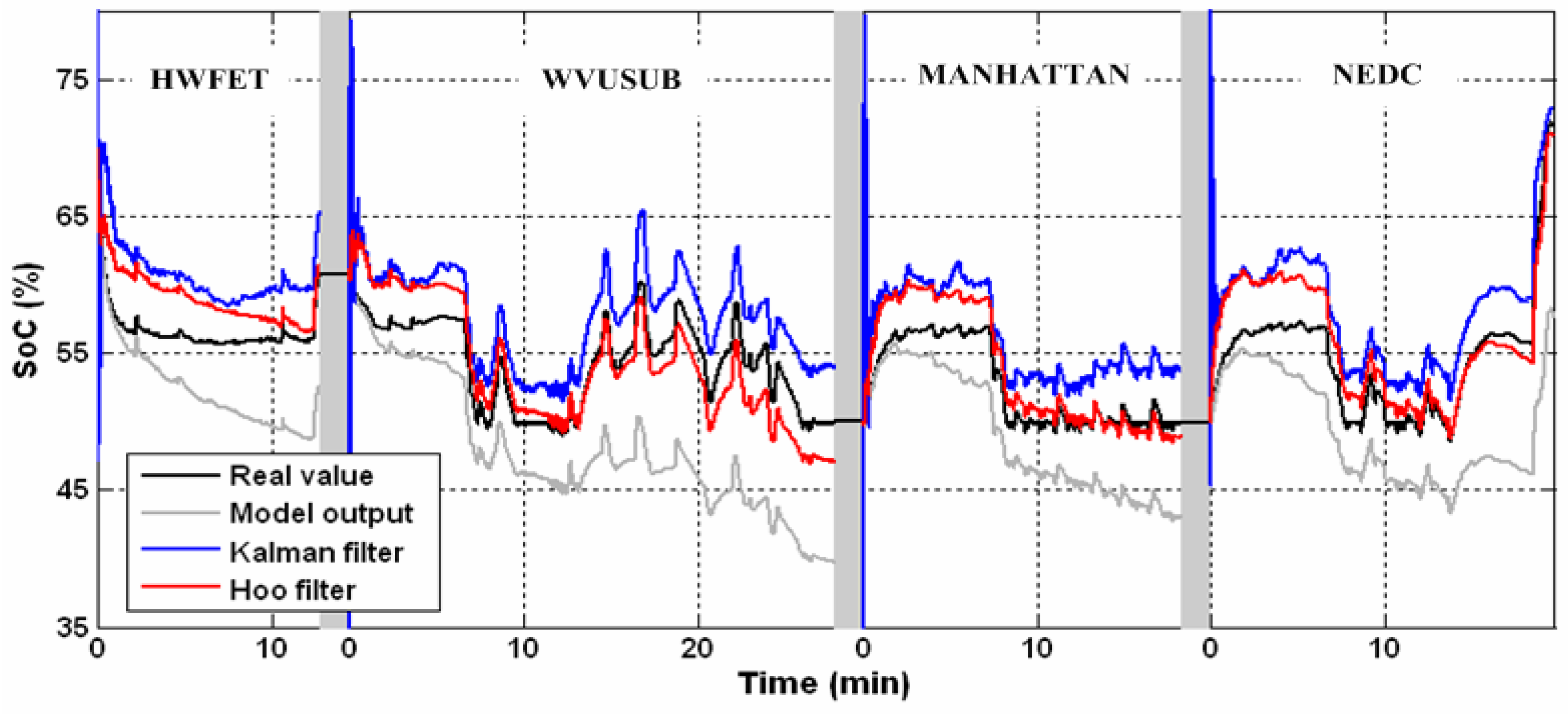
To demonstrate the performance of H${}_{\infty }$ filter, simulation experiments are conducted to compare the SoC estimation errors among model output, result of Kalman filter and result of H${}_{\infty }$ filter.

As demonstrated above, adaptive-κ nonlinear diffusion filter has the ability to remove the current noise and self-learning strategy can compensate the zero-drift. Therefore, we fix the SNR of current noise to 10 dB and zero-drift to 0.5 A, which simulates the residual noises after the two noise reduction steps. The experiments aims at verifying the filters’ abilities to handle the modeling error, thus we apply a fixed model with parameters setting to their maximum, average, and minimum values of each cycle respectively. The inaccurate model parameters includes the resistances of $R_b$,$R_s$,$R_o$ and capacitance of $C_c$. Since $C_b$ is determined by the nominal capacity of battery, rather than identification, no modeling error is added to it.

Battery model parameters are from the Panasonic Prismatic 6.5 Ah battery. The settings for Kalman filter are experimentally optimized as initial states estimation error $P=0.01I$, process noise variance matrix $Q={0.001}^{2}I$, and measurement noise variance matrix $R={0.01}^2$. The settings for H${}_{\infty }$ filter are $L=[1,1]$ and $\gamma =50$. If γ fails to satisfy the condition equation (26), it will increase 10 step by step till meets the requirement.

Figure 8 shows the SoC estimation results of Prius successively driving on HWFET, WVUSUB, MANHATTAN, and NEDC driving cycles. Due to the non-zero mean of current noise and model error, the accumulated errors totally are reflected on the model output, resulting a nonconvergent estimation result. After a short time of oscillation, Kalman filter gradually converges to a stable estimation, however, with stable errors. Zero-drift and model errors destroy its conditions to be an optimal filter. H${}_{\infty }$ leads to a faster convergence process than Kalman filter and achieves smaller stable errors.

Table 3 summarizes the numerical results. Obviously H${}_{\infty }$ filter has the ability to estimate SoC of the time-variant battery based on a set of fixed parameters. It outperforms Kalman filter no matter which values the model parameters are fixed to. The robustness of H${}_{\infty }$ filter is well demonstrated.

5. Data Fusion and System Overall Performance

From the results shown in Figure 5 and Figure 8, it is clear that coulomb counting usually has good estimation at the beginning period due to small accumulated errors, while the H${}_{\infty }$ filter obtain better performance in the latter period when it reaches convergent estimation. Therefore, one natural way to make the best use of the advantages and bypass the disadvantages is to combine the results of two estimators, weighting by time.

In the proposed framework, we design a simple data fusion unit to achieve the final SoC estimation $\widehat{SoC}\left(k\right)$ based on linear combination of $\widehat{So{C}_1}\left(k\right)$ and $\widehat{So{C}_2}\left(k\right)$. The weights of the two estimators are expressed as the following equations, experimentally determined using trial and error method.

$$\widehat{SoC}\left(k\right)=\left\{\begin{array}{c}\widehat{So{C}_1}\left(k\right)t\le 5\hfill \\ {\omega }_1\times \widehat{So{C}_1}\left(k\right)+{\omega }_1\times \widehat{So{C}_2}\left(k\right)5<t<10\hfill \\ \widehat{So{C}_2}\left(k\right)t\ge 10\hfill \end{array}\right.$$

(34)

where ${\omega }_1=-0.2t+2$, ${\omega }_2=0.2t-1$ and t is the vehicle running time (unit [min]).

Figure 8. SoC estimation results based on inaccurate battery model using the fixed average values of real time-variant parameters (white noise with 10dB SNR and 0.5A zero-drift). The gray bars between cycles represent half-hour stops which allow OCV available.

Figure 8. SoC estimation results based on inaccurate battery model using the fixed average values of real time-variant parameters (white noise with 10dB SNR and 0.5A zero-drift). The gray bars between cycles represent half-hour stops which allow OCV available.

Table 3. Performance comparison of SoC estimation based on battery model using a set of fixed parameters (Unit [%]). The inaccurate model parameters include resistances of $R_e$, $R_t$, $R_o$ and capacitance of $C_c$, and are fixed to the their maximum, average and minimum values in each driving cycle respectively. White noises with 10dB SNR and 0.5A zero-drift are also added to the real current profile.

Fix model parameters to	Highway (HWFET)				Suburban (WVUSUB)				Urban (MANHATTAN)				European hybrid (NEDC)
	Kalman Filter		H${}_{\infty }$ filter		Kalman Filter		H${}_{\infty }$ filter		Kalman Filter		H${}_{\infty }$ filter		Kalman Filter		H${}_{\infty }$ filter
	ave	std	ave	std	ave	std	ave	std	ave	std	ave	std	ave	std	ave	std
Max. of parameters	4.38	1.41	2.92	2.03	3.99	1.44	1.71	1.59	4.00	1.98	1.35	2.32	3.57	1.22	1.60	1.61
Ave. of parameters	4.34	2.22	2.47	1.21	3.56	1.48	1.94	2.20	3.71	1.88	1.55	1.42	3.82	1.85	1.93	1.83
Min. of parameters	3.77	3.73	1.50	1.15	3.20	1.20	1.78	2.01	3.92	2.24	2.15	2.19	3.90	1.58	2.22	2.34

Table 3. Performance comparison of SoC estimation based on battery model using a set of fixed parameters (Unit [%]). The inaccurate model parameters include resistances of $R_e$, $R_t$, $R_o$ and capacitance of $C_c$, and are fixed to the their maximum, average and minimum values in each driving cycle respectively. White noises with 10dB SNR and 0.5A zero-drift are also added to the real current profile.

Fix model parameters to	Highway (HWFET)				Suburban (WVUSUB)				Urban (MANHATTAN)				European hybrid (NEDC)
	Kalman Filter		H${}_{\infty }$ filter		Kalman Filter		H${}_{\infty }$ filter		Kalman Filter		H${}_{\infty }$ filter		Kalman Filter		H${}_{\infty }$ filter
	ave	std	ave	std	ave	std	ave	std	ave	std	ave	std	ave	std	ave	std
Max. of parameters	4.38	1.41	2.92	2.03	3.99	1.44	1.71	1.59	4.00	1.98	1.35	2.32	3.57	1.22	1.60	1.61
Ave. of parameters	4.34	2.22	2.47	1.21	3.56	1.48	1.94	2.20	3.71	1.88	1.55	1.42	3.82	1.85	1.93	1.83
Min. of parameters	3.77	3.73	1.50	1.15	3.20	1.20	1.78	2.01	3.92	2.24	2.15	2.19	3.90	1.58	2.22	2.34

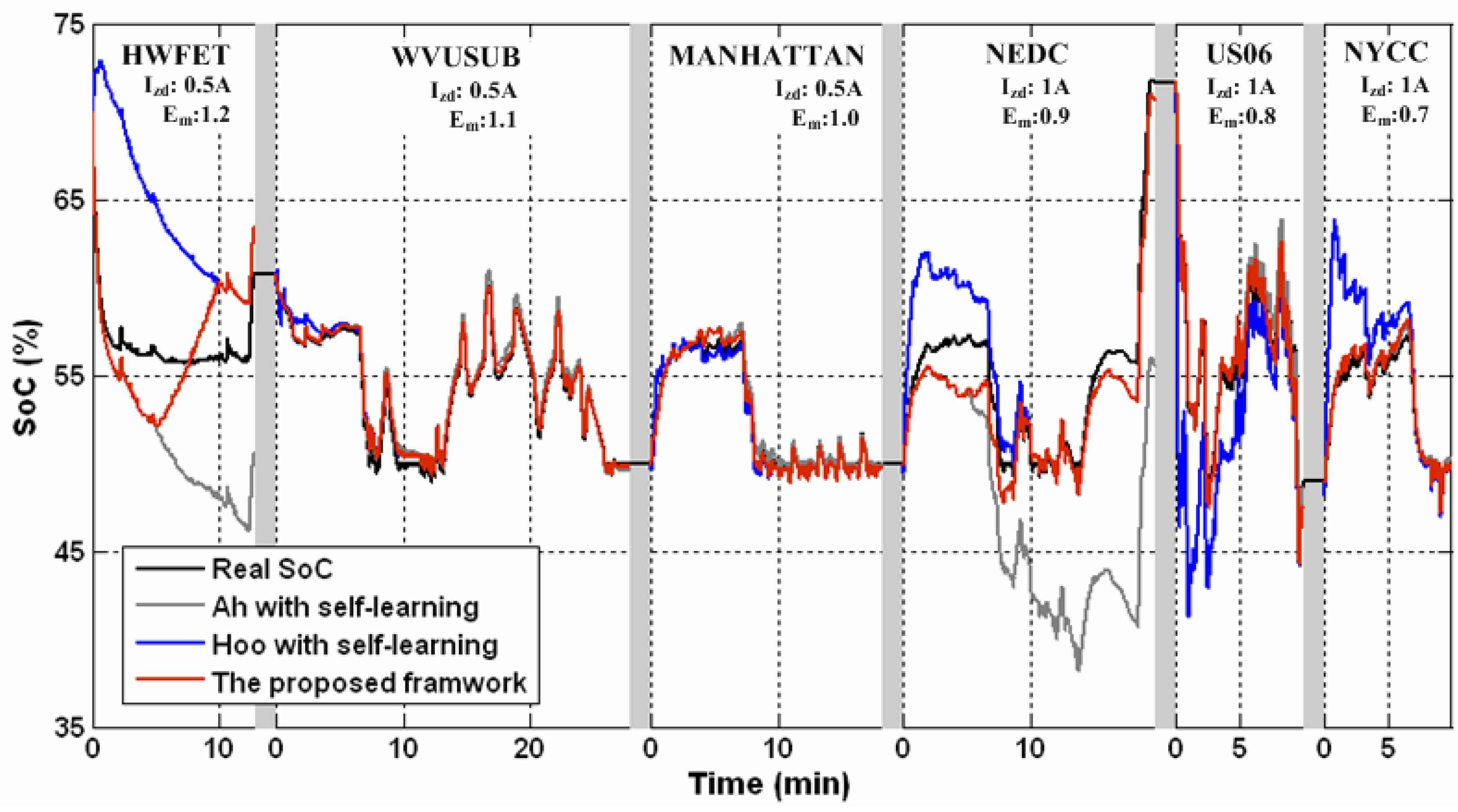
Since we have demonstrated coulomb counting with self-learning strategy outperforms conventional method and H${}_{\infty }$ filter achieves more robust estimation than Kalman filter in real vehicle driving environment, the verification of availability and efficacy of the overall framework only requires to compare its performance with the two single estimator.

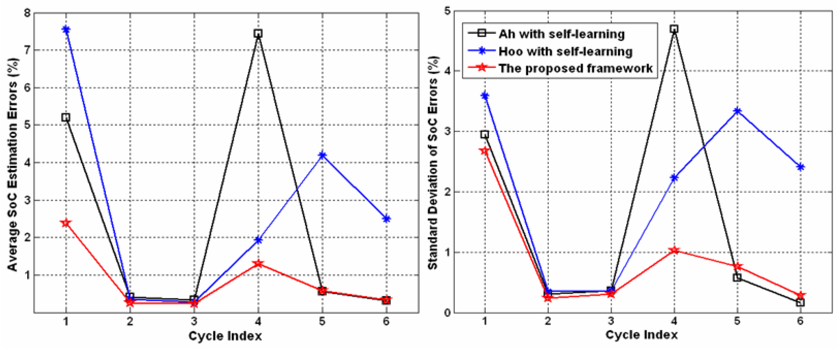
The simulation environment is the same as the experiments given above. The SNR of white current noise is fixed to 5dB and the zero-drift is set to 0.5A for the first 3 cycles and changed to 1A for the other ones. To further test the robustness of the whole framework, we introduce the model error ($E_m$) defined as: $E_m=p_m/p_r$, where $p_m$ is the model parameter, $p_r$ is the real parameter, p presents the arbitrary parameters of $R_o$, $R_s$, $R_b$ and $C_c$. The $E_m$ varies from 1.2 in the 1st cycle to 0.7 in the last cycle.

The estimation results are shown in Figure 9 and Figure 10 gives the averages of absolute estimation errors and their standard deviations in each cycle. In the first cycle of HWFET, the zero-drift in measurement of current as well as the model error results in the large error in coulomb counting and H${}_{\infty }$ filter. The fusion of the two approaches can reduce such error. In the following two cycles, self-learning strategy estimates the zero-drift and compensates the error effectively. Although the other two approaches also show good performance, the hybrid approach outperforms them. In the forth cycle, the drift is enlarged. The errors of H${}_{\infty }$ filter and coulomb counting are the largest in the first 1/3 and latter 2/3 sections respectively, while the hybrid approach has the least error. In the last two cycles, self-learning estimates the zero-drift again. Consequently, Ah method performance is improve. Even though the model error is enlarged, due to it robustness, H${}_{\infty }$ filter converges to a small error after passing through a short period of large-error region so that the fusion results still keep in good performance.

Figure 9. SoC estimation results of self-learning coulomb counting, H${}_{\infty }$ filter and the overall framework (white noise with 5dB SNR, zero-drift 0.5A for the 1st-3rd cycles and 1A for the 4th-6th cycles, model error changes from 1.2 to 0.7). The gray bars between cycles represent half-hour stops which allow OCV available.

Figure 9. SoC estimation results of self-learning coulomb counting, H${}_{\infty }$ filter and the overall framework (white noise with 5dB SNR, zero-drift 0.5A for the 1st-3rd cycles and 1A for the 4th-6th cycles, model error changes from 1.2 to 0.7). The gray bars between cycles represent half-hour stops which allow OCV available.

As a summary, the performance of coulomb counting and H${}_{\infty }$ filter are dependent on the model error, noise and zero-drift. Although they have slightly better performance in some region, the overall performance by the hybrid method is the best among them.

6. Conclusions and Future Works

Noises produced by all kinds of interference in vehicle driving environment, zero-drifts caused by sensors and measurement circuits, and model uncertainties due to the strong time-variant property of batteries are incompatible with the prerequisites of the typical SoC estimation methods, such as coulomb counting and model-based methods. Therefore, it is necessary to study the abilities of anti-noise and self-adaption of SoC estimation and enhance estimation robustness in the presence of non-ideal conditions.

In this study, we have proposed a framework to implement robust estimation of SoC in the application of EVs. Firstly, the proposed adaptive-κ nonlinear diffusion filter has the ability to estimate the SNR of noisy signal and reduce noises according to the degree of change. Since it catches the main difference in characters of real signal and measured noises, it outperforms linear digital filter and wavelet based filter. The zero-drift in the measurement of current then is estimated using the estimation error of coulomb counting at each SoC calibration available moment. This self-learning strategy works simply because the accumulated error is mainly attributed to the non-zero mean of noise. H${}_{\infty }$ filter is also introduced to realize the robust estimation using a fixed model. Although the fixed model can not fully predict the dynamics of a time-variant battery, the inherent robustness of H${}_{\infty }$ filter successfully handles the model uncertainty and the estimation gradually converges to stable tracking with small errors. Considering the good performance of coulomb counting method at the early phase due to small accumulated errors and the small stable estimation errors of H${}_{\infty }$ after a period of convergence process, the data fusion unit rationally and efficiently integrates the results of them with the time-dependant weights. The availabilities and effectiveness of single components and overall framework have been demonstrated by comparative studies with conventional approaches, under the testing conditions of noises with various signal-noise-ratios, varying zero-drifts, and different model errors.

Figure 10. Numerical indexes of SoC estimation results of self-learning coulomb counting, H${}_{\infty }$ filter and the overall framework (white noise with 5dB SNR, zero-drift 0.5A for the 1st-3rd cycles and 1A for the 4th-6th cycles, model error changes from 1.2 to 0.7). The left subfigure shows average absolute estimation error while the right subfigure illustrates their standard deviation.

Figure 10. Numerical indexes of SoC estimation results of self-learning coulomb counting, H${}_{\infty }$ filter and the overall framework (white noise with 5dB SNR, zero-drift 0.5A for the 1st-3rd cycles and 1A for the 4th-6th cycles, model error changes from 1.2 to 0.7). The left subfigure shows average absolute estimation error while the right subfigure illustrates their standard deviation.

In the future, we will apply the SoC estimation framework into some real electric vehicles. It is also necessary to collect the statistic properties of noises, zero-drifts and model errors in vehicle driving environment so that mathematical analysis of robustness of this framework can be further studied.