A Microscale Modeling Tool for the Design and Optimization of Solid Oxide Fuel Cells

Abstract
:
1. Introduction
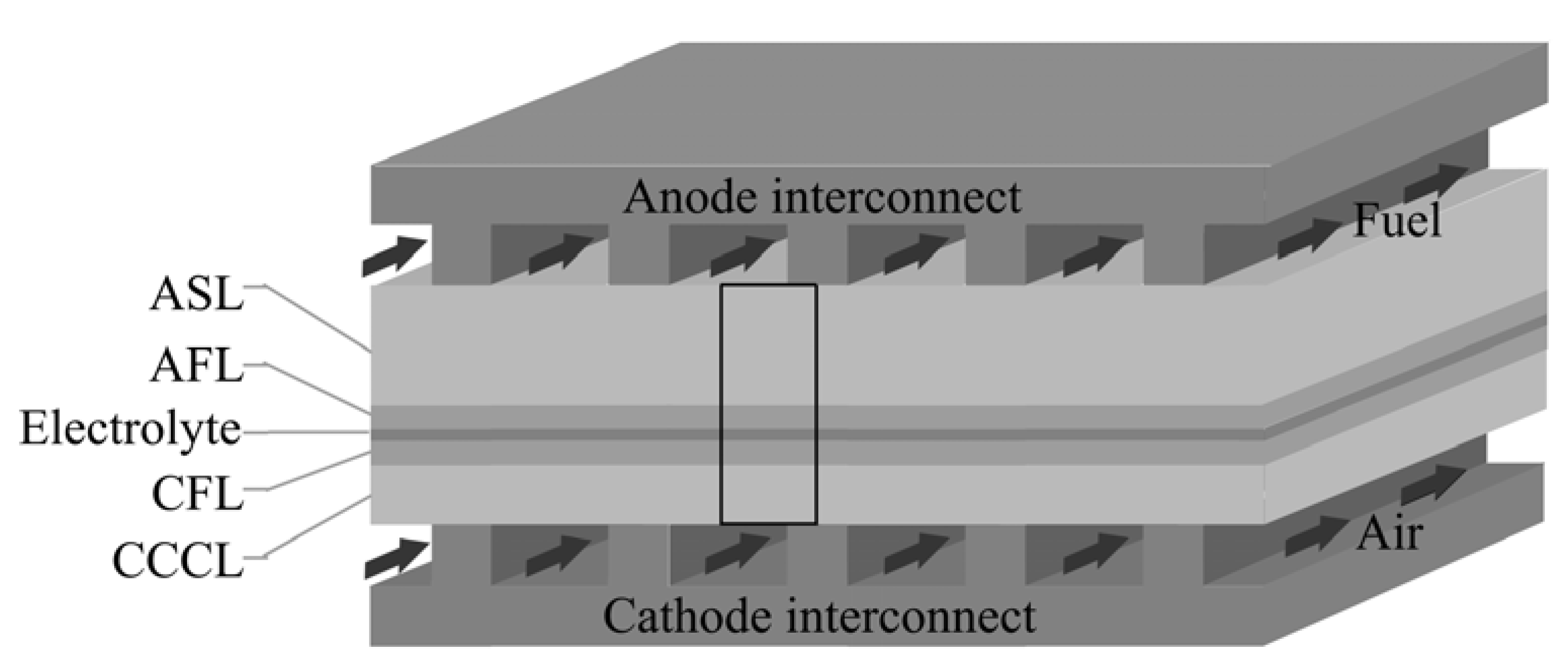
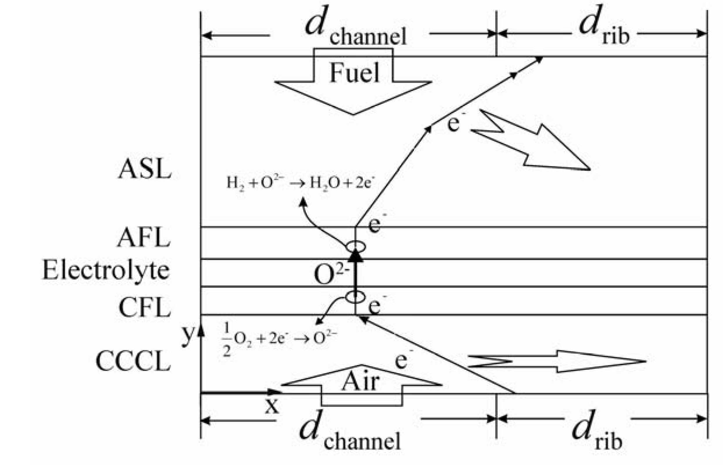
2. Method

| Parameters | Value |
|---|---|
| Cell temperature, T (°C) | 700 |
| Inlet fuel/air pressure, Patm (Pa) | 1.013 × 10⁵ |
| Cell output voltage, Vop (V) | 0.7 |
| ASL thickness, lASL (μm) | 1,000 |
| AFL thickness, lAFL (μm) | 20 |
| Electrolyte thickness, lYSZ (μm) | 8 |
| CFL thickness, lCSL (μm) | 20 |
| CCCL thickness, lCCCL (μm) | 50 |
| Porosity, | 0.48 (ASL), 0.23 (AFL), 0.26 (CFL), 0.45 (CCCL) |
| Ni volume fraction, | 0.55 (ASL, AFL) |
| LSM volume fraction, | 0.475 (CFL), 1 (CCCL) |
| Tortuosity, | 3 |
| Angle of particle contact, (o) | 30 |
| Bruggeman factor, m | 1.5 |
| Mean particle diameter, dp (μm) | 1 (ASL, CCCL), 0.5 (AFL, CFL) |
| Electrical conductivity of Ni, (s m-1) | |
| Electrical conductivity of LSM, (s m-1) | |
| Ionic conductivity of YSZ, (s m-1) | |
| Diffusion volume of H2, (m3 mol-1) | 7.07 × 10⁻⁶ |
| Diffusion volume of H2O, (m3 mol-1) | 12.7 × 10⁻⁶ |
| Diffusion volume of O2, (m3 mol-1) | 16.6 × 10⁻⁶ |
| Diffusion volume of N2, (m3 mol-1) | 17.9 × 10⁻⁶ |
| Molar mass of H2, (kg mol-1) | 2 × 10⁻³ |
| Molar mass of H2O, (kg mol-1) | 18 × 10-3 |
| Molar mass of O2 , (kg mol-1) | 32 × 10-3 |
| Molar mass of N2 , (kg mol-1) | 28 × 10-3 |
| Permeability of anode (m2) | 7.93 × 10⁻¹⁶ |
| Permeability of cathode (m2) | 3.06 × 10⁻¹⁶ |
| Viscosity of fuel (Pa s) | 2.8 × 10⁻⁵ |
| Viscosity of air (Pa s) | 4 × 10⁻⁵ |
| Knudsen diffusion coefficient of H2 (m2 s-1) | 4.37 × 10⁻⁴ |
| Knudsen diffusion coefficient of H2O (m2 s-1) | 1.46 × 10⁻⁴ |
| Knudsen diffusion coefficient of O2 (m2 s-1) | 7.64 × 10⁻⁵ |
| Knudsen diffusion coefficient of N2 (m2 s-1) | 8.17 × 10⁻⁵ |
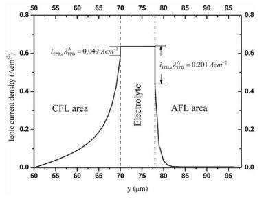
2.1. Electrochemical Reactions in AFL and CFL
2.2. Gas Transport in Porous Electrode
2.2.1. Dusty gas model
2.2.2. Governing equations
2.3. Electrical Conduction
2.4. Boundary Conditions (BCs)
| Equations | Boundary | ASL/channel interface | AFL/Electrolyte interface | All others | ||||
| Fuel transfer | BC Type | H2 molar concentration | H2O molar concentration | H2 inward molar flux | H2O inward molar flux | Insulation/Symmetry | ||
| BC | ||||||||
| Boundary | CCCL/channel interface | CFL/Electrolyte interface | All others | |||||
| Air transfer | BC Type | O2 molar concentration | N2 molar concentration | O2 inward molar flux | N2 inward molar flux | Insulation/Symmetry | ||
| BC | 0 | |||||||
| Equations | Boundary | Rib/CCCL interface | Rib/ASL interface | CFL/Electrolyte interface | AFL/Electrolyte interface | All others |
| Electronic transfer | BC Type | Reference potential | Reference potential | Inward current flow | Inward current flow | Electric insulation |
| BC | Vcell- | 0 | ||||
| Ionic transfer | BC Type | Interior current source | Interior current source | Electric insulation | ||
| BC |
2.5. Numerical Method
3. Results and Discussion
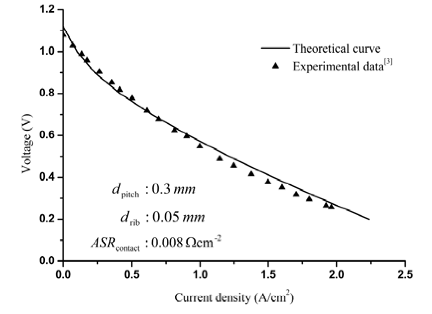
3.1. Model Fitting of the Experimental I-V Curve
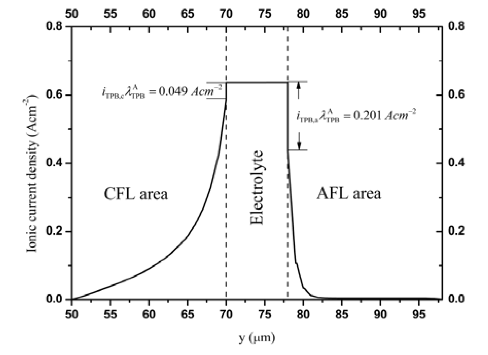
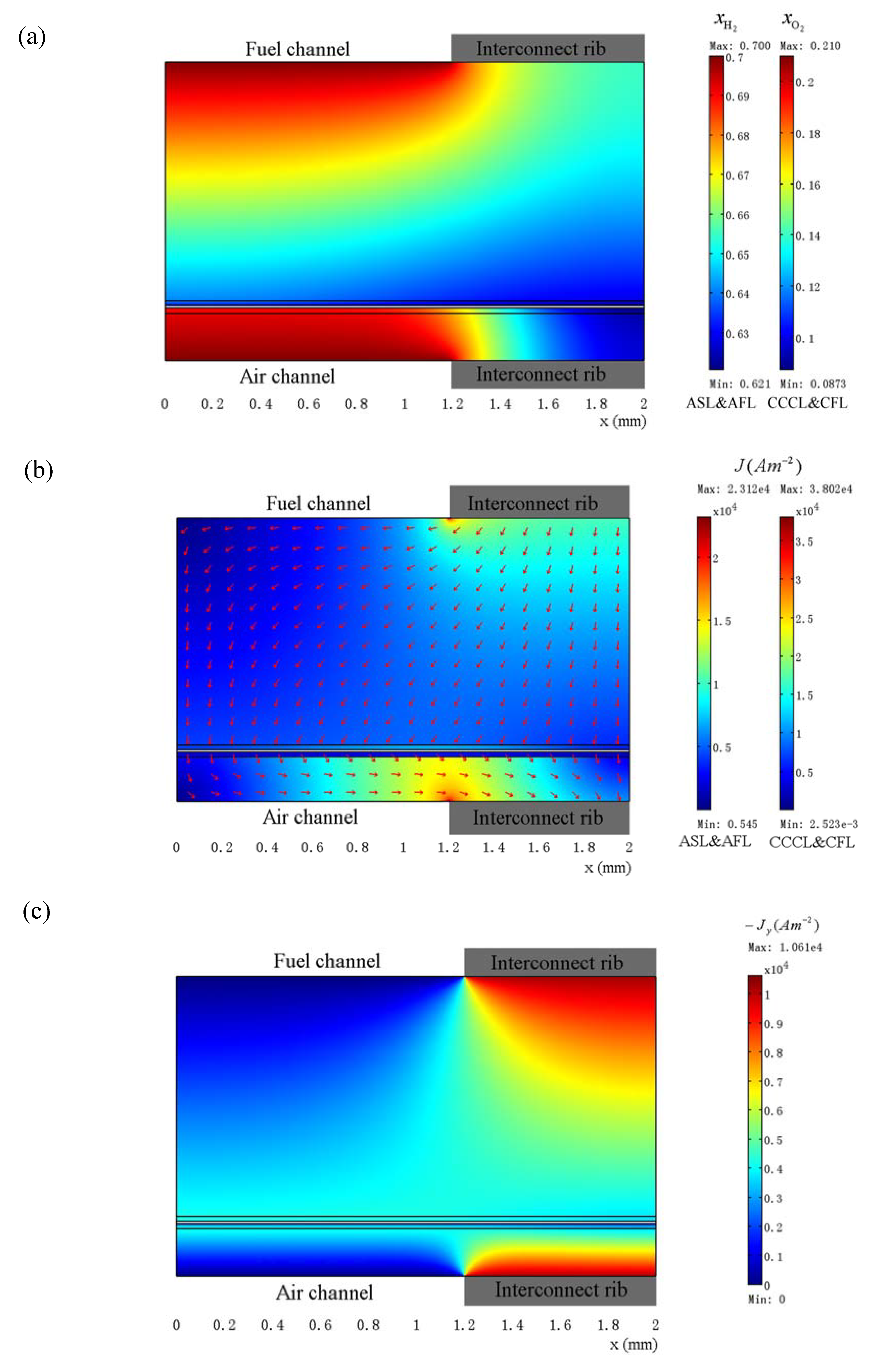
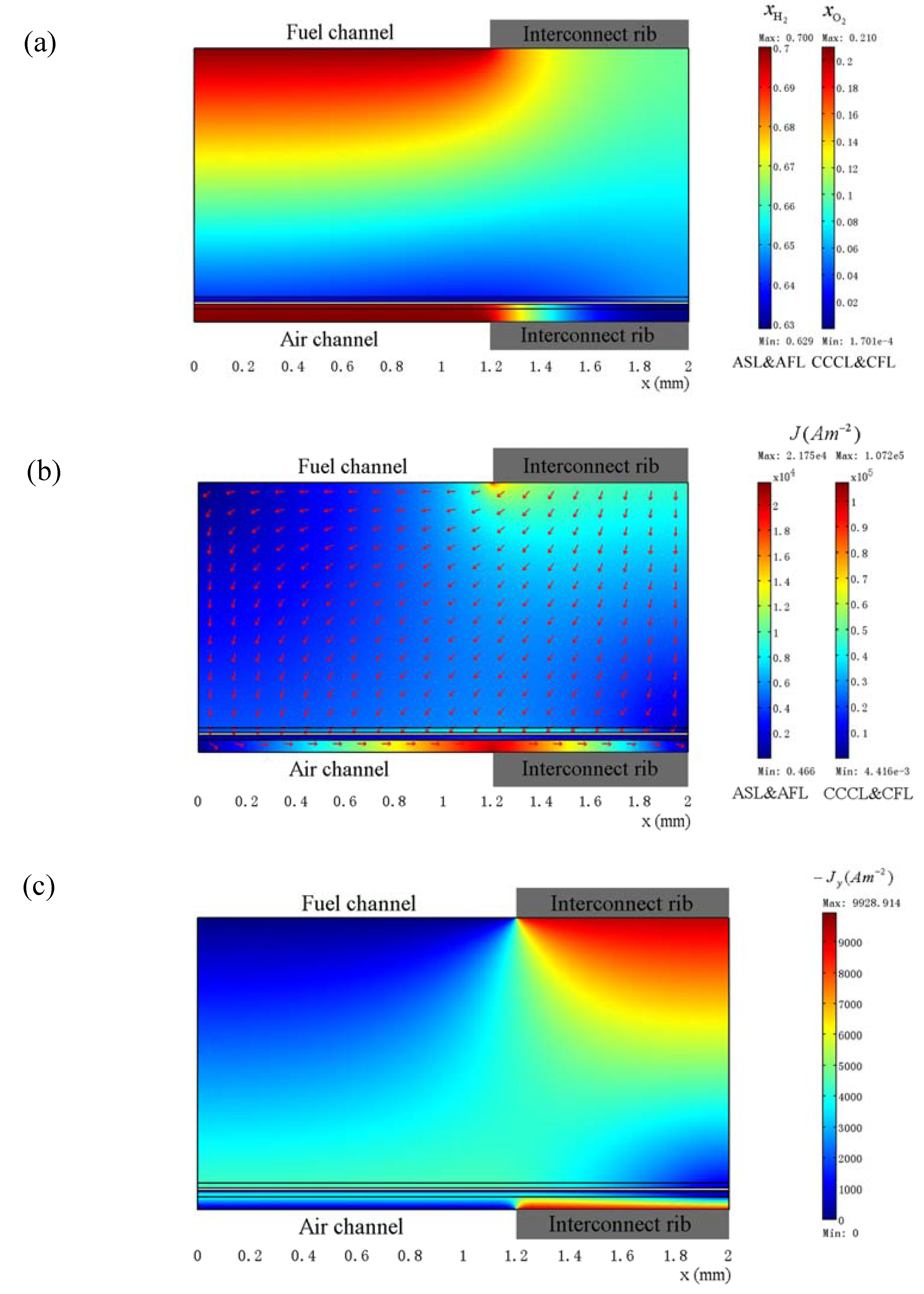
3.2. Distributions of Physical Quantities in Stack Cell

3.3. Optimization of Geometry Parameters
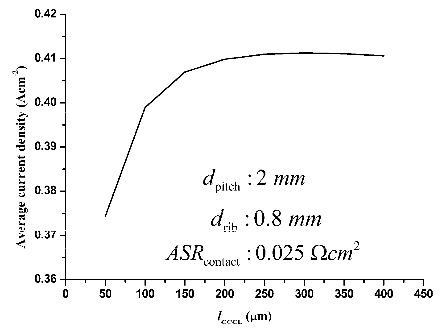
3.3.1. Optimization of the CCCL thickness

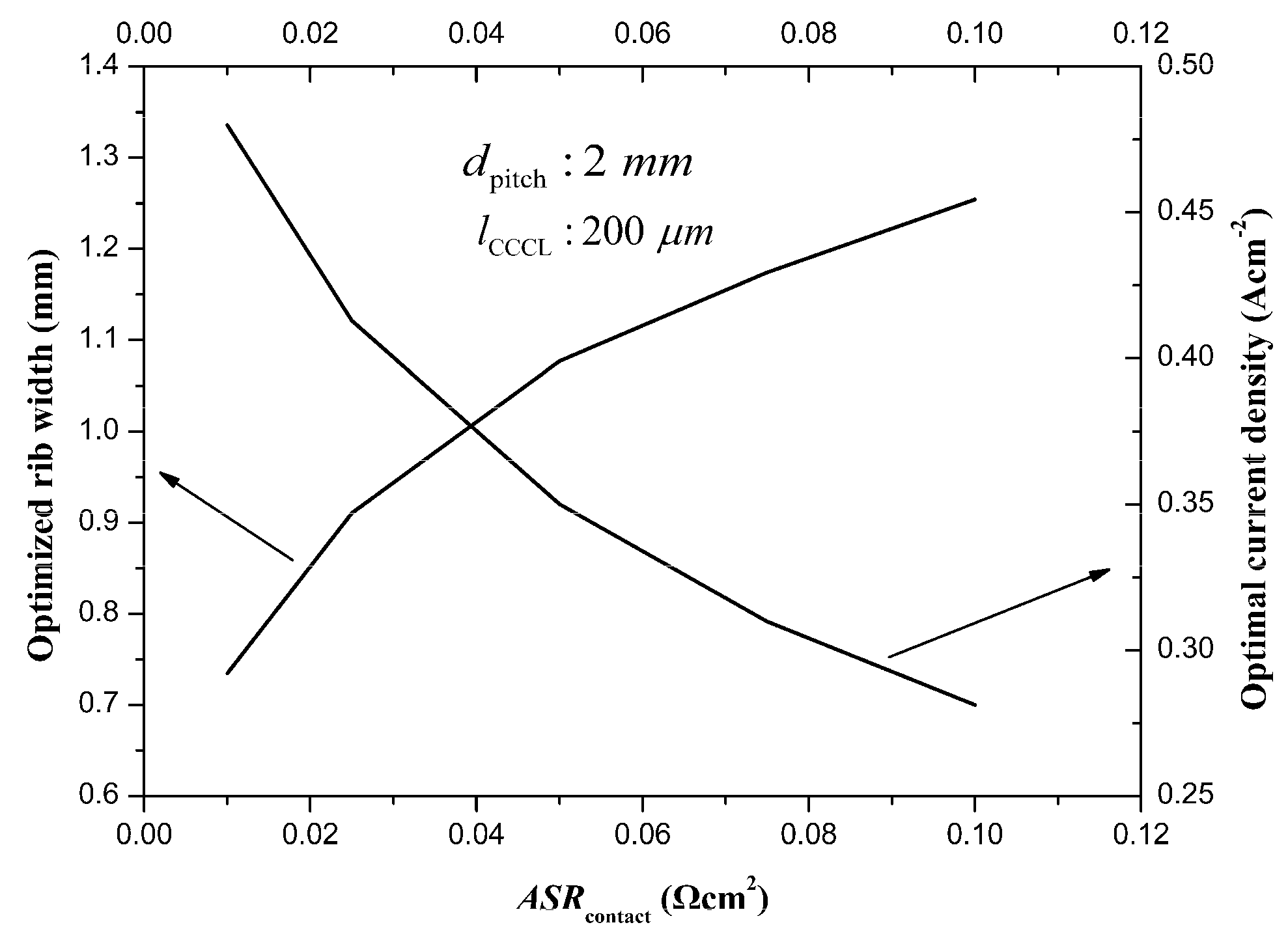
3.3.2. Optimization of the rib width

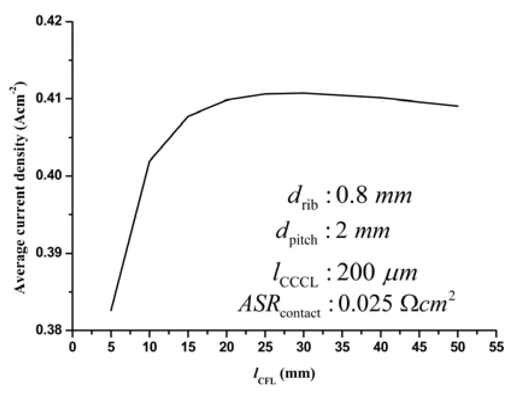
3.3.3. Optimization of the CFL thickness
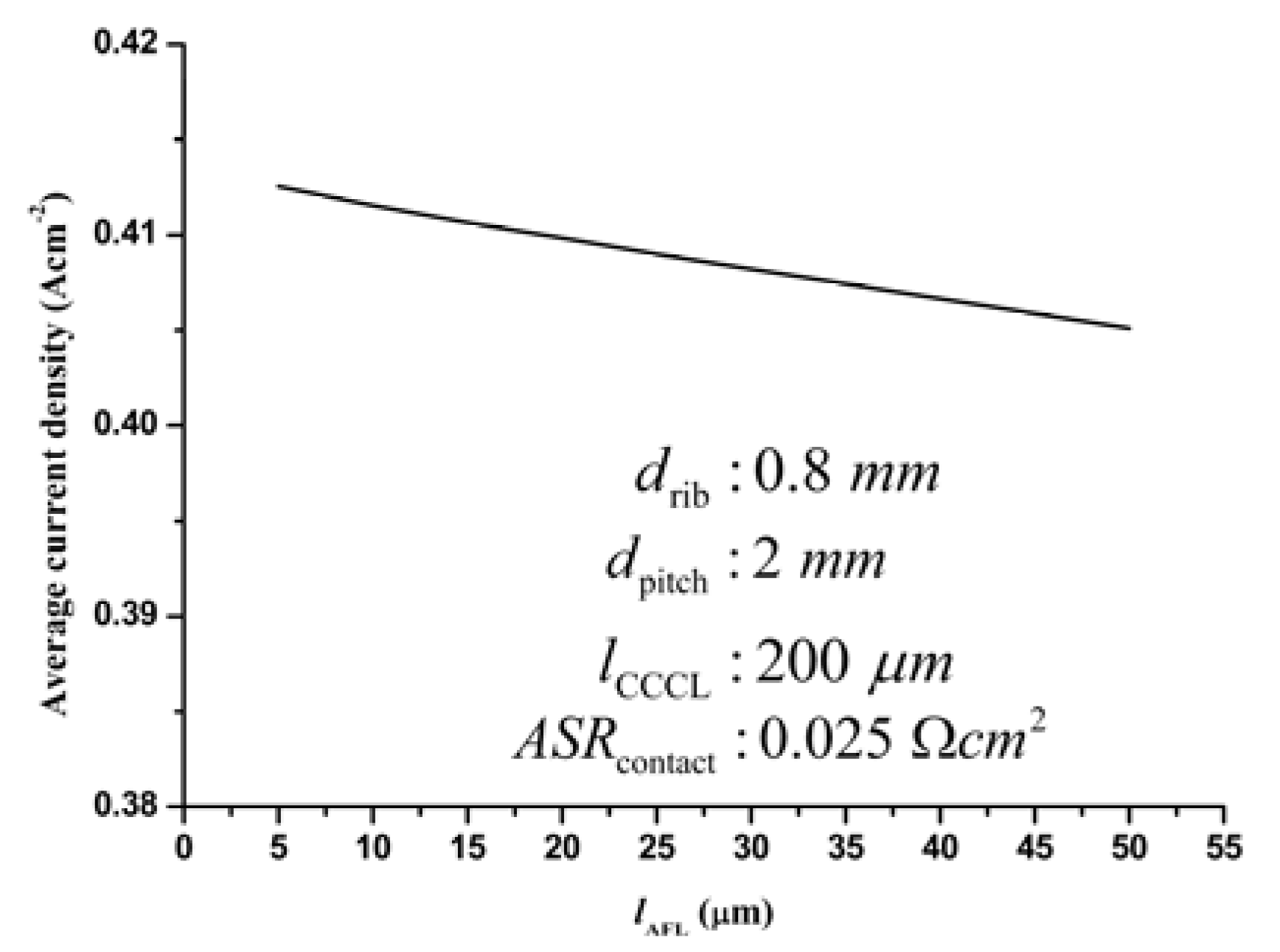
3.3.4. Optimization of the AFL thickness

4. Conclusions
Acknowledgements
References and Notes
- Kim, J.W.; Virkar, A.V.; Fung, K.Z.; Mehta, K.; Singhal, S.C. Polarization effect in intermediate temperature, anode-supported solid oxide fuel cell. J. Electrochem. Soc. 1999, 146, 69–78. [Google Scholar] [CrossRef]
- EG&G Technical Services, Inc. Fuel cell handbook, 7th ed.U.S. Department of Energy: Morgantown, WV, USA, 2004.
- Zhao, F.; Virkar, A.V. Dependence of polarization in anode-supported solid oxide fuel cells on various cell parameters. J. Power Sources 2005, 141, 79–95. [Google Scholar] [CrossRef]
- Haanappel, V.A.C.; Mertens, J.; Rutenbeck, D.; Tropartz, C.; Herzhof, W.; Sebold, D.; Tietz, F. Optimisation of processing and microstructural parameters of LSM cathodes to improve the electrochemical performance of anode-supported SOFCs. J. Power Sources 2005, 141, 216–226. [Google Scholar] [CrossRef]
- Basu, R.N.; Blass, G.; Buchkremer, H.P.; Stover, D.; Tietz, F.; Wessel, E.; Vinke, I.C. Simplified processing of anode-supported thin film planar solid oxide fuel cells. J. Eur. Ceram. Soc. 2005, 25, 463–471. [Google Scholar] [CrossRef]
- Moon, H.; Kim, S.D.; Park, E.W.; Hyun, S.H.; Kim, H.S. Characteristics of SOFC single cells with anode active layer via tape casting and co-firing. Int. J. Hydrogen Energy 2008, 33, 2826–2833. [Google Scholar] [CrossRef]
- Leone, P.; Santarelli, M.; Asinari, P.; Calì, M.; Borchiellini, R. Experimental investigations of the microscopic features and polarization limiting factors of planar SOFCs with LSM and LSCF cathodes. J. Power Sources 2008, 177, 111–122. [Google Scholar] [CrossRef]
- Liu, S.; Song, C.; Lin, Z. The effects of the interconnect rib contact resistance on the performance of planar solid oxide fuel cell stack and the rib design optimization. J. Power Sources 2008, 183, 214–225. [Google Scholar] [CrossRef]
- Lin, Z.; Stevenson, J.W.; Khaleel, M.A. The effect of interconnect rib size on the fuel cell concentration polarization in planar SOFCs. J. Power Sources 2003, 117, 92–97. [Google Scholar] [CrossRef]
- Suwanwarangkul, R.; Croiset, E.; Fowler, M.W.; Douglas, P.L.; Entchev, E.; Douglas, M.A. Performance comparison of Fick’s, dusty-gas and Stefan-Maxwell models to predict the concentration overpotential of a SOFC anode. J. Power Sources 2003, 122, 9–18. [Google Scholar] [CrossRef]
- Khaleel, M.A.; Lin, Z.; Singh, P.; Surdoval, W.; Collins, D. A finite element analysis modeling tool for solid oxide fuel cell development: coupled electrochemistry, thermal and flow analysis in MARC®. J. Power Sources 2004, 130, 136–148. [Google Scholar] [CrossRef]
- Zhu, H.; Kee, R.J.; Janardhanan, V.M.; Deutschmann, O.; Goodwin, D.G. Moleling elementary heterogeneous chemistry and electrochemistry in solid-oxide fuel cells. J. Electrochem. Soc. 2005, 152, A2427–A2440. [Google Scholar] [CrossRef]
- Khaleel, M.A.; Rector, D.R.; Lin, Z.; Johnson, K.; Recknagle, K.P. Multiscale electrochemistry modeling of solid oxide fuel cells. Int. J. Multiscale Comput. Eng. 2005, 3, 33–48. [Google Scholar] [CrossRef]
- Suwanwarangkul, R.; Croiset, E.; Entchev, E.; Charojrochkul, S.; Pritzker, M.D.; Fowler, M.W.; Douglas, P.L.; Chewathanakup, S.; Mahaudom, H. Experimental and modeling study of solid oxide fuel cell operating with sysgas fuel. J. Power Sources 2006, 161, 308–322. [Google Scholar] [CrossRef]
- Bove, R.; Ubertini, S. Modeling solid oxide fuel cell operation: approaches, techniques and results. J. Power Sources 2006, 19, 543–559. [Google Scholar] [CrossRef]
- Bi, W.; Chen, D.; Lin, Z. A key geometric parameter for the flow uniformity in planar solid oxide fuel cell stacks. Int. J. Hydrogen Energy 2009, 34, 3873–3884. [Google Scholar] [CrossRef]
- Jeon, D.H.; Nam, J.H.; Kim, C.J. Microstructural optimization of anode-supported solid oxide fuel cells by a comprehensive microscale model. J. Electrochem. Soc. 2006, 153, A406–A417. [Google Scholar] [CrossRef]
- Kenney, B.; Karan, K. Engineering of microstruture and design of planar porous composite SOFC cathode: A numerical analysis. Solid State Ionics 2007, 178, 297–306. [Google Scholar] [CrossRef]
- Ho, T.X.; Kosinski, P.; Hoffmann, A.C.; Vik, A. Numerical modeling of solid oxide fuel cells. Chem. Eng. Sci. 2008, 63, 5356–5365. [Google Scholar] [CrossRef]
- Tseronis, K.; Kookos, I.K.; Theodoropoulos, C. Modelling mass transport in solide oxide fuel cell anodes: a case for a multidimensional dusty gas-based model. Chem. Eng. Sci. 2008, 63, 5626–5638. [Google Scholar] [CrossRef]
- Chen, D.; Lin, Z.; Zhu, H.; Kee, R.J. Percolation theory to predict effective properties of solid oxide fuel-cell composite electrodes. J. Power Sources 2009, 191, 240–252. [Google Scholar] [CrossRef]
- Krishna, R.; Wesselingh, J.A. The Maxwell-Stefan approach to mass transer. Chem. Eng. Sci. 1997, 52, 861–991. [Google Scholar] [CrossRef]
- Young, J.B.; Todd, B. Modelling of multi-component gas flows in capillaries and porous solids. Int. J. Heat Mass Transfer 2005, 48, 5338–5353. [Google Scholar] [CrossRef]
- Todd, B.; Young, J.B. Thermodynamic and transport properties of gases for use in solid oxide fuel cell modeling. J. Power Sources 2002, 110, 186–200. [Google Scholar] [CrossRef]
- Fuller, E.N.; Schettler, P.D.; Giddings, J.C. A new method of prediction of binary gas-phase diffusion coefficients. Ind. Eng. Chem. 1966, 58, 18–27. [Google Scholar]
- COMSOL Multiphysics® Version 3.4 User’s Guide; COMSOL AB.: Los Angeles, CA, USA, 2007.
© 2009 by the authors; licensee MDPI, Basel, Switzerland. This article is an open-access article distributed under the terms and conditions of the Creative Commons Attribution license (http://creativecommons.org/licenses/by/3.0/).
Share and Cite
Liu, S.; Kong, W.; Lin, Z. A Microscale Modeling Tool for the Design and Optimization of Solid Oxide Fuel Cells. Energies 2009, 2, 427-444. https://doi.org/10.3390/en20200427
Liu S, Kong W, Lin Z. A Microscale Modeling Tool for the Design and Optimization of Solid Oxide Fuel Cells. Energies. 2009; 2(2):427-444. https://doi.org/10.3390/en20200427
Chicago/Turabian StyleLiu, Shixue, Wei Kong, and Zijing Lin. 2009. "A Microscale Modeling Tool for the Design and Optimization of Solid Oxide Fuel Cells" Energies 2, no. 2: 427-444. https://doi.org/10.3390/en20200427