An Improved Frequency Dead Zone with Feed-Forward Control for Hydropower Units: Performance Evaluation of Primary Frequency Control

1
The state key Laboratory of Water Resources and Hydropower Engineering Science, Wuhan University, Wuhan 430072, China
2
School of Power and Mechanical Engineering, Wuhan University, Wuhan 430072, China
3
China Southern Power Grid Power Generation Company, Guangzhou 510630, China
*
Author to whom correspondence should be addressed.
Energies 2019, 12(8), 1497; https://doi.org/10.3390/en12081497
Submission received: 22 February 2019
/
Revised: 15 April 2019
/
Accepted: 16 April 2019
/
Published: 20 April 2019
Abstract
:Due to the integration of more intermittent renewable energy into the power grid, the demand for frequency control in power systems has been on the rise, and primary frequency control of hydropower units plays an increasingly important role. This paper proposes an improved frequency dead zone with feed-forward control. The aim is to achieve a comprehensive performance of regulating rapidity, an assessment of integral quantity of electricity, and the wear and tear of hydropower units during primary frequency control, especially the unqualified performance of integral quantity of electricity assessment under frequency fluctuations with small amplitude. Based on a real hydropower plant with Kaplan units in China, this paper establishes the simulation model, which is verified by comparing experimental results. After that, based on the simulation of real power grid frequency fluctuations and a real hydropower plant case, the dynamic process of primary frequency control is evaluated for three aspects, which include speed, integral quantity of electricity, and wear and tear. The evaluation also includes the implementations of the three types of dead zones: common frequency dead zone, the enhanced frequency dead zone, and the improved frequency dead zone. The results of the study show that the improved frequency dead zone with feed-forward control increases the active power output under small frequency fluctuations. Additionally, it alleviates the wear and tear problem of the enhanced frequency dead zone in the premise of guaranteeing regulation speed and integral quantity of electricity. Therefore, the improved frequency dead zone proposed in this paper can improve the economic benefit of hydropower plants and reduce their maintenance cost. Accordingly, it has been successfully implemented in practical hydropower plants in China.
1. Introduction
In recent years, the advancement of renewable energy generation technology has facilitated the integration of more and more renewable energy, such as wind energy and solar energy, into the power grid. This has further changed the power grid gradually towards the direction of flexible power systems [1,2]. The integration of these new renewable energy sources has also made the structure of the power grid more complex, consequently increasing the demand for frequency regulation of the power grid [3,4]. As a renewable energy (aside from generation), hydropower significantly shoulders a large portion of the regulation and balancing duty in many power systems. As such, hydropower regulation is crucial in the frequency stability of power grids [5,6,7,8,9].
The regulation of active power output in the primary frequency control (PFC) of hydropower units is among the main methods of maintaining the frequency stability of power grids [9]. Few regions in the world have an explicit ancillary service market to procure PFC services because its costs are difficult to identify; however, new market design for PFC services are being actively explored [9,10,11,12]. Regarding the quality of PFC process, different countries tend to have different assessment mechanisms [9,13]. Countries and regions with mature electricity markets, such as Europe, North America, and Oceania, have widely adopted the ancillary service compensation mechanisms of frequency and voltage control [13,14,15]. In China, however, the electricity market has not yet been completed, and the standard market mechanisms have not been fully formed, even though China has been developing in recent years [16,17,18]. For the active power regulation in PFC, the rapidity of regulation is considered an important indicator for the power grids all over the world. A large number of previous researchers have studied the fast regulation performance of hydropower units [19,20,21,22,23]. In addition, China’s power grid has an important assessment indicator—integral quantity of electricity (IQE). IQE is the superposition of active power adjustments of generating units in the process of frequency disturbance of power grids. The IQE of a hydropower unit directly reflects the PFC performance and relates to the frequency stability of the power grid. If the hydropower plants (HPP) have unqualified IQE assessment, the relevant power grid organizations will impose fines on them, reduce the electrical load of power plants in the overall dispatch, and even close down generation units for some small hydropower plants. This directly affects the power generation profit and the development of the HPPs.
Other than the IQE assessment of regulating quality and the increasing demand for PFC of hydropower units, the problem of tear and wear of hydropower units has also become one of the indicators that cannot be ignored in PFC, as it directly affects the life of the units [24]. In essence, the core of hydropower unit wear is the coordination between the power producers and the power grids [24,25]. To maintain the relative stability of the power grid frequency, it is necessary to control the active power of generation units. Similarly, the most appropriate way to control the active power of generation units is the regulation of guide vane opening, which leads to the wear and tear. For power grids with dramatical and frequent frequency fluctuations, wear is likely to be more serious. Some previous studies explored the wear on bearing materials of guide vanes of hydropower turbines [26,27,28]. In addition, other studies were conducted on fatigue design and life of Francis turbine runners [4,29,30,31,32]. Some previous studies also examined the loss, financial impacts, and maintenance cost of wear in the regulation process of hydropower units [33,34,35,36,37,38,39]. Other studies researched the assessment methods of wear and tear in detail [24,25].
To study the frequency fluctuations of power grids in more detail, the frequency fluctuations amplitude of 7000 s in the Hubei power grid of China was counted, as illustrated in Figure 1 and Figure 2, which show the real frequency of 7000 s. From the statistical results, it is observable that the frequency fluctuations of the power grid are mostly below 0.1 Hz, which belongs to a small frequency fluctuation. Also, it is evident that when the frequencies are within the range of 50 ± 0.05 Hz, they belong to a reasonable range. Hence, the regulators usually set the common frequency dead zone in the process of PFC [40]. This dead zone is generally set in 0.05 Hz in the requirement of the power grid. The dead zone setting can effectively filter frequency fluctuations that are less than the set value of the dead zone, thus reducing the actions of the regulator. Still, when the frequency fluctuations exceed the dead zone setting value, the difference between the grid frequency and the given frequency will be deducted from the dead zone setting value. As such, when this kind of dead zone is disturbed by small frequency fluctuations, the calculated frequency differences will be generally small. In addition to the effect of the mechanical dead zone and the power dead zone of the servo system, the movements of the guide vane regulation are small or even unnoticeable. Due to this, the active power regulation quantities of the unit are lower than the IQE assessment, which subsequently leads to the insufficient power contribution of PFC and the unqualified IQE.
Since some hydropower units have insufficient active powers, and the IQE is unqualified, some scholars have proposed an enhanced frequency dead zone to improve the integrated power in the previous studies [41]. The enhanced frequency dead zone is introduced in Section 2. This method improves the active power regulation of the units under small frequency fluctuations. It also improves the response speed of PFC. However, owing to its characteristics, the wear of the units is greatly increased, which ultimately affects the life of the unit. This paper proposes an improved frequency dead zone to address the shortcomings of the common frequency dead zone and the enhanced frequency dead zone for hydropower units. In addition, a feed-forward control is introduced in the regulator model to make sure that the PFC is regulated to the target power value as well as to improve the active power output. Based on the real grid frequency fluctuations of 7000 s and the real hydropower plant example, this paper comprehensively evaluates the performance of different frequency dead zones from three aspects: regulation speed, IQE, and unit wear and tear.
The content of this paper is organized as follows: Section 2 introduces the specific algorithm of the common, the enhanced, and the improved frequency dead zones, the feed-forward control principle, the MATLAB/Simulink modeling method, and the assessment indicator of regulation quality. In addition, the paper offers the basic information and the specific parameters of the studied HPP. Section 3 verifies the simulation model. After that, Section 4 analyzes the dynamic process and assesses the regulation quality of the three kinds of dead zone algorithms. Finally, Section 5 presents the conclusion of the paper.
2. Method
2.1. The Improved Frequency Dead Zone and Feed-Forward Control
For the traditional PFC, the regulator utilizes the common frequency dead zone. The algorithm is as shown below:
where
- represents the given frequency,
- is the grid frequency,
- represents the set value of frequency dead zone [20].
sets in the regulator, which can effectively filter frequency fluctuations that are less than the set value of the dead zone. It can reduce unnecessary actions of the regulator.
According to formula (1) and Figure 3, when the absolute value of the difference between the given frequency and the gird frequency of the system is less than the set value of the frequency dead zone, the frequency difference after calculation of the dead zone will be 0, while the regulating system will not act. Similarly, when the absolute value of the difference is greater than the set value of the frequency dead zone, that is, if the difference is greater than 0, then the frequency difference after calculation of the dead zone will be the difference between the given frequency and the grid frequency of the system minus the artificial set value of the frequency dead zone. Also, if the difference is less than 0, the difference is between the given frequency and the grid frequency of the system plus the artificial set value of the frequency dead zone. This means that when the frequency of the power grid fluctuates near the set value of the dead zone, the frequency difference calculated by the common frequency dead zone will be small. Therefore, the vane movement of the servo system will be small as well. In addition to the impact of the mechanical dead zone and the power dead zone, among others, the power output change is small or even unchanged. This results in an unqualified IQE in the assessment of the power plant.
To address the problem of small active power regulation resulting from too small a frequency difference in the regulation process, some scholars have recently proposed an enhanced frequency dead zone algorithm to artificially increase the frequency difference and output of active power. The algorithm is as shown in formula (2):
where
- represents the given frequency,
- is the grid frequency,
- represents the set value of frequency dead zone [41].
According to formula (2) and Figure 4, regarding the enhanced frequency dead zone algorithm, when the absolute value of the difference between the given frequency and the grid frequency is less than the set value of the frequency dead zone, the frequency difference after the dead zone will be 0. Also, when the absolute value of the difference between the given frequency and the power grid frequency is greater than the set value of frequency dead zone, the frequency difference after the dead zone will increase the set value of the dead zone by a step change compared with the common frequency dead zone. In this sense, the difference of the regulator calculated in Proportion Integration Differentiation (PID) will be increased. Thus, the regulation movement of the servo system and the active power output of PFC will be increased as well. Still, there is a disadvantage. When the frequency difference exceeds the set value of the dead zone, the regulation quantity of PFC will be larger, and the speed of regulation will be faster. Therefore, the wear of the servo system will be more obvious than that of the common frequency dead zone in the regulation process. Accordingly, if the system frequency fluctuates near the set value of the frequency dead zone over a long period, the frequent movements will occur in PFC, which has a negative impact on the life of hydropower units.
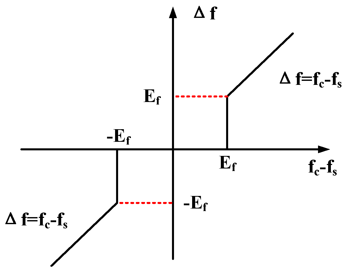
Considering the shortcomings of the enhanced frequency dead zone, this paper proposes an improved frequency dead zone. The frequency difference algorithm is as shown in formula (3):
In formula (3), represents the set value of the frequency dead zone, which varies with time; , decreases with a certain slope k, and the initial value is .
According to formula (3) and Figure 5, different from the enhanced frequency dead zone, the improved frequency dead zone demonstrates that when the difference between the given frequency and the grid frequency exceeds the set value of the frequency dead zone, the initial frequency difference will not be a step change. Instead, it will increase with time at a certain rate. Consequently, when an active power is regulated by the servo system, the regulation quantity is gradually increased. This prevents the unit from adjusting too fast, thus avoiding frequent movements of the unit and reducing its wear. Compared with the common dead zone, the improved dead zone can also increase the frequency differences of regulator in the regulation process, which means that the servo system will get regulating signals with larger amplitude than the normal frequency dead zone, thus increasing the active power output and improving the response of frequency change.
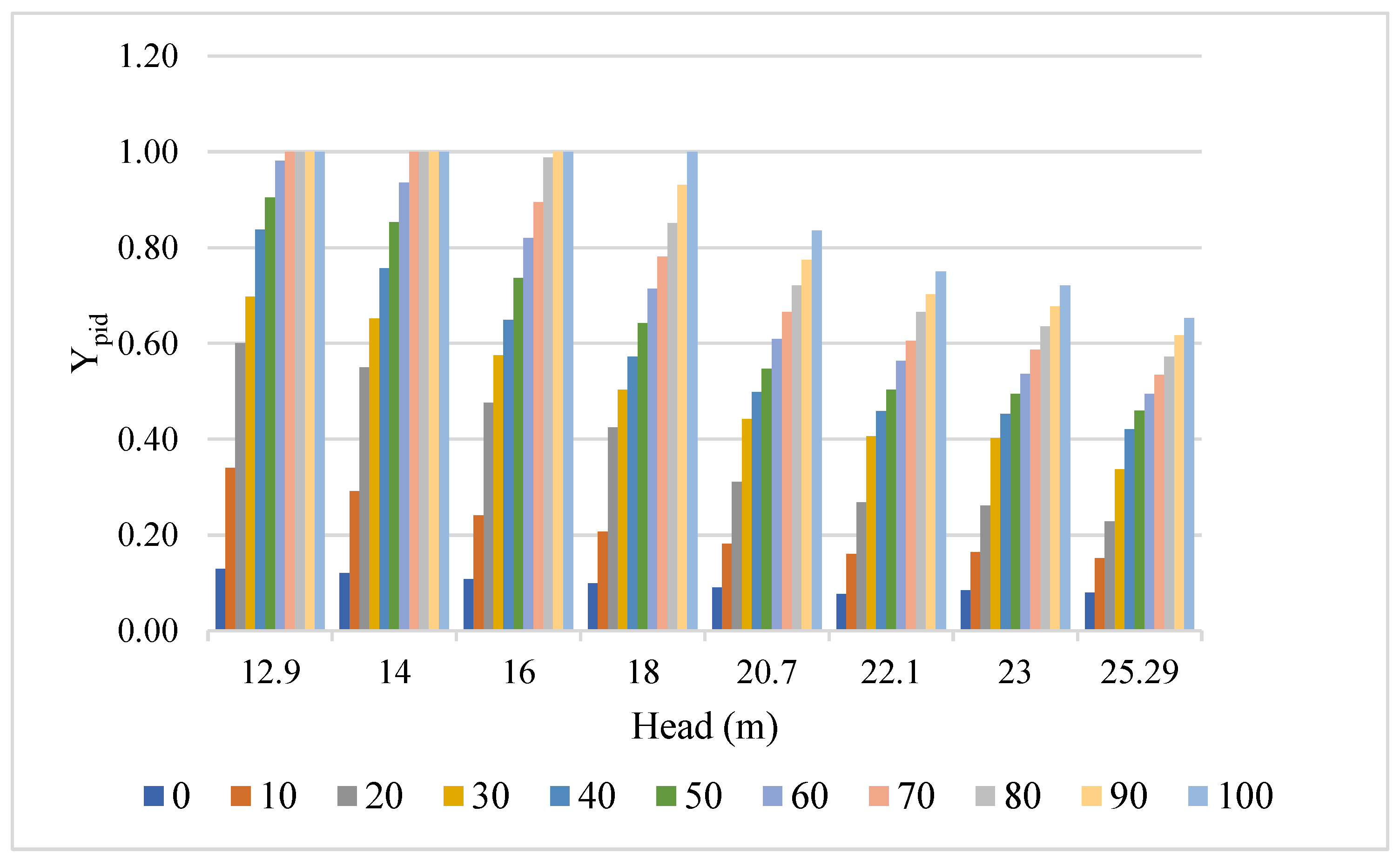
In addition to the improved frequency dead zone, the regulator model incorporates the feed-forward control. When the unit runs under power mode, the regulator cannot adjust to the target power value due to the impact of the power dead zone, which results in an unqualified IQE. Therefore, to ascertain the output of active power, the feed-forward control method is introduced to compensate the regulation of PID. In particular, the principle of feed-forward control is to compensate the disturbance action in advance as per the disturbance quantity after the disturbance is generated. It also ensures the regulation accuracy and response speed. Through interpolation fitting, the steady output values of the regulator Ypid are obtained when the hydropower unit runs steadily under different water heads with different loads. These compensation quantities are superimposed with the PID to increase the output signal of the regulator. As a result, the output of the servo system is increased to ensure that the unit reaches the power target values under different heads. Additionally, the IQEs are increased. Figure 6 indicates a regulator model that contains feed-forward control. In the process of model simulation, the feed-forward control part can interact with the PID or not participate in the simulation. Table A1 shows the Ypid values of feed-forward control under different water heads and power values. Figure A1 shows the fitting of the feed-forward diagram.
2.2. Modeling
This paper is based on a Chinese HPP with a Kaplan turbine. It uses a MATLAB/Simulink software (Mathworks, Natick, MA, USA) to establish the regulation system model, mainly including regulator model, servo system model, turbine and water diversion system model, as well as generation model. Selective control mode of power and frequency is adopted in the regulation, which is discussed in detail under Section 2.2.2.
2.2.1. Basic Mathematical Model
The regulator is part of the governor and is used for the regulation of hydropower units. It adopts the PID control. The transfer function is shown in formula (4):
where
- is the transfer function of regulator,
- is proportional gain,
- is integral gain,
- is differential gain,
- represents the differential time constant [42].
is used to suppress high frequency interference and overcome the weak regulating effect of differential part of PID control. The regulator model established in this paper is displayed in Figure 6. The common, enhanced, and improved frequency dead zones are set before the PID algorithm, respectively. Only one of them can be selected for dynamic analysis in the simulation calculation.
The servo system is utilized to convert the PID regulating signal into the mechanical signal, which is aimed to control the opening of the guide vane. Its mathematical model is as shown in formula (5):
where
- is the transfer function of the servo system,
- is the relay response time constant [19].
can be considered as the time taken by the relay to complete its journey when the distributing valve opening is 100%.
When the turbine adopts a rigid water hammer and a unit water diversion system model, the transfer function is expressed in formula (6):
where
- is the transfer function of turbine,
- is the transfer coefficient of turbine torque to vane opening,
- is the flow inertia time constant,
- represents the transfer coefficient of flow to water head [19],
- ; is the transfer coefficient of turbine flow to vane opening; is the transfer coefficient of turbine torque to head.
can be understood as the time required to accelerate the flow of water in the pipeline to the rated flow rate at the rated head. The dynamic characteristics of the turbine are often expressed by the torque characteristics and flow characteristics under steady-state conditions. Additionally, the turbine characteristic curve and the flying escape characteristic curve are widely used presently as the test curves obtained by the turbine at steady states.
Torque characteristics are shown in formula (7):
Flow characteristics are shown in formula (8):
where
- is the turbine torque,
- is the turbine flow,
- is the guide vane opening,
- is the unit speed,
- is the water head,
- represents the blade angle.
When building the turbine model, the model can be built as per the specific model characteristic curve data of the actual power station. This ensures that the model can better reflect the actual characteristics of the turbine [43].
When the generator adopts the first-order mathematical model, the transfer function is expressed in formula (9):
where
- is the transfer function of generator,
- is the unit mechanical inertia time constant,
- is the comprehensive self-regulation coefficient of the hydro-generator set.
2.2.2. Regulation Mode Selection
The main running modes of the unit regulation system are the opening and the power modes. In the power mode, the regulator utilizes the given power as the instruction signal and the output power of the unit as the feedback. For the statistics of PFC, the PFC performance in the power mode is considered to be better than that in the opening mode. In particular, when the unit is integrated into the large power grid, it can achieve the coordination between PFC and AGC (automatic generation control) load setting, because when units are running in the power mode, PFC can change the power output according to the current power and the given power. Meanwhile, during the regulating process, AGC may issue new given power instructions according to the load of the power grid, which makes the regulation signals the superposition of PFC and AGC, and the regulation system can reach the new balance. While it is difficult to achieve the coordination in the opening mode, the power dispatching department usually requires the power station to adopt the power mode to regulate. Therefore, when the model is established, the regulating system opts to operate in the power mode. The main power modes of the regulating system are the integrated control mode of frequency and power (ICFP) and the selective control mode of frequency and power (SCFP).
Figure 7 shows that the ICFP uses the same controller to control power and frequency. In addition, there are two feedbacks in the controller. One is the unit frequency, while the other is the active power output of the unit. Figure 8 shows that the SCFP uses different controllers for power and frequency control. Controller one has a frequency feedback, while controller two is used for power control and has two feedbacks—one is the unit frequency, and the other is the active power output. When the hydropower unit is connected to the large power grid, the unit has little impact on the grid frequency when regulating active power regulation. In this case, from the standpoint of automatic control, frequency regulation is considered an open-loop system without feedback. At the same time, the frequency of the unit varies very little. Additionally, the active power output of the unit can be considered the same as the torque output of the turbine. Thus, the change in the system frequency can be equivalent to a change in a given frequency, and a drop in the unit frequency can be regarded as a rise in a given frequency.
The transfer function of ICPF is expressed in formula (10):
Without considering the differential term, the formula can be simplified as formula (11):
Subsequently, the characteristic equation can be expressed as formula (12):
We assume that the characteristic equation is as formula (13):
where
- ,
- ,
- ,
- .
Assuming that the root of the characteristic equation is , and , the transfer function can be expressed as formula (14):
Under the action of step disturbance with a given frequency, the Laplace transformation of the moment can be expressed as formula (15):
The time domain response process of the moment signal is obtained by taking the Laplace transform as formula (16):
Thus, as long as the system poles, and have negative real parts, x(t) will have a certain steady-state value after a certain period, especially when the system is stable. At the same time, the poles may be all real poles or contain conjugate complex poles. Thus, the decay process of P (t) may be a monotonous decay process or an oscillation decay process over time.
Since the Laplace transformation of the moment can be expressed as formula (17):
is considered the dominant pole. As such, the estimated value of the frequency signal implementation time is as formula (18):
From formula (18), regulation time is connected with three parameters: , and .
As well, the transfer function of SCFP is expressed as formula (19):
The same method is utilized for simplification as ICFP, in which the estimated value of implementation time of frequency instruction signal is expressed as formula (20):
From formula (20), regulation time is unconcerned with .
As such, when SCFP is applied, the regulation time will only be concerned with and , which can reduce related parameters.
2.3. Evaluating Approach
For the regulation performance of hydropower units, the common frequency dead zone, the enhanced frequency dead zone, and the improved frequency dead zone are mainly measured using three indicators: IQE, regulation speed, and servo system wear and tear.
2.3.1. IQE
IQE reflects the regulation of active power in the case of frequency fluctuations. Additionally, it is a crucial reference for power grid dispatching agencies to assess the regulation quality of power plant units, which mainly includes theoretical IQE and practical IQE. The theoretical IQE is calculated from the frequency fluctuations that exceed the set value of frequency dead zone. It is expressed as formula (21):
where
- is the rated power of the unit.
The formula of practical IQE is expressed as formula (22):
where
- is the active power of the unit at any time t in the effective time,
- represents the active power of the unit at the initial time.
If the frequency of the power grid returns to the set value of the frequency dead zone within 60 s, the integration will end. The integration time is regarded as the time when the frequency difference returns to the set value of the frequency dead zone. Otherwise, the integration time will be 60 s [41].
In assessing active power, if the practical IQE is more than 50% of its theoretical IQE, then the PCF is considered to be qualified.
2.3.2. Regulation Rapidity
This paper seeks to evaluate the response speed of power regulation through lag time and response time in the process of power regulation under step disturbance. The lag time of PFC denotes the time taken by the unit from the beginning of the frequency disturbance of the power grid to the active power regulation of the unit to 2% of the difference between the original active power and the stable active power. On the other hand, the primary frequency response time refers to the time from the grid frequency crossing the dead zone of the unit frequency to the maximum load adjustment of the theoretical primary frequency modulation of 90%. In essence, the response time is among the indices used to evaluate the quality of primary frequency regulation in the power grid. In China, for instance, when the units operate on 80% of the rated load, the power response for 60 s frequency step ought to meet a series of requirements as per the specifications of the China Electricity Council. That is, the response time should not be more than 15 s. Also, for hydropower plants with water head greater than 50 m, the lag time of the unit in the regulation process should not be more than 4 s. In addition, for hydropower plants with water head less than 50 m, the lag time of the unit in the regulation process should not be more than 8 s [19,21,44].
2.3.3. Wear and Tear of Hydropower Units
With the increasingly complex structure of the power grid along with the incorporation of more and more renewable energy into the power grid, the frequency regulation times of hydropower units have increased dramatically. As such, the wear and tear of hydropower units cannot be ignored in the regulation process. In reference to [24,25], this paper seeks to measure the wear and tear of hydropower units by counting the number of actions of servomotors as well as the magnitude of each action under the real frequency.
2.4. Study Case
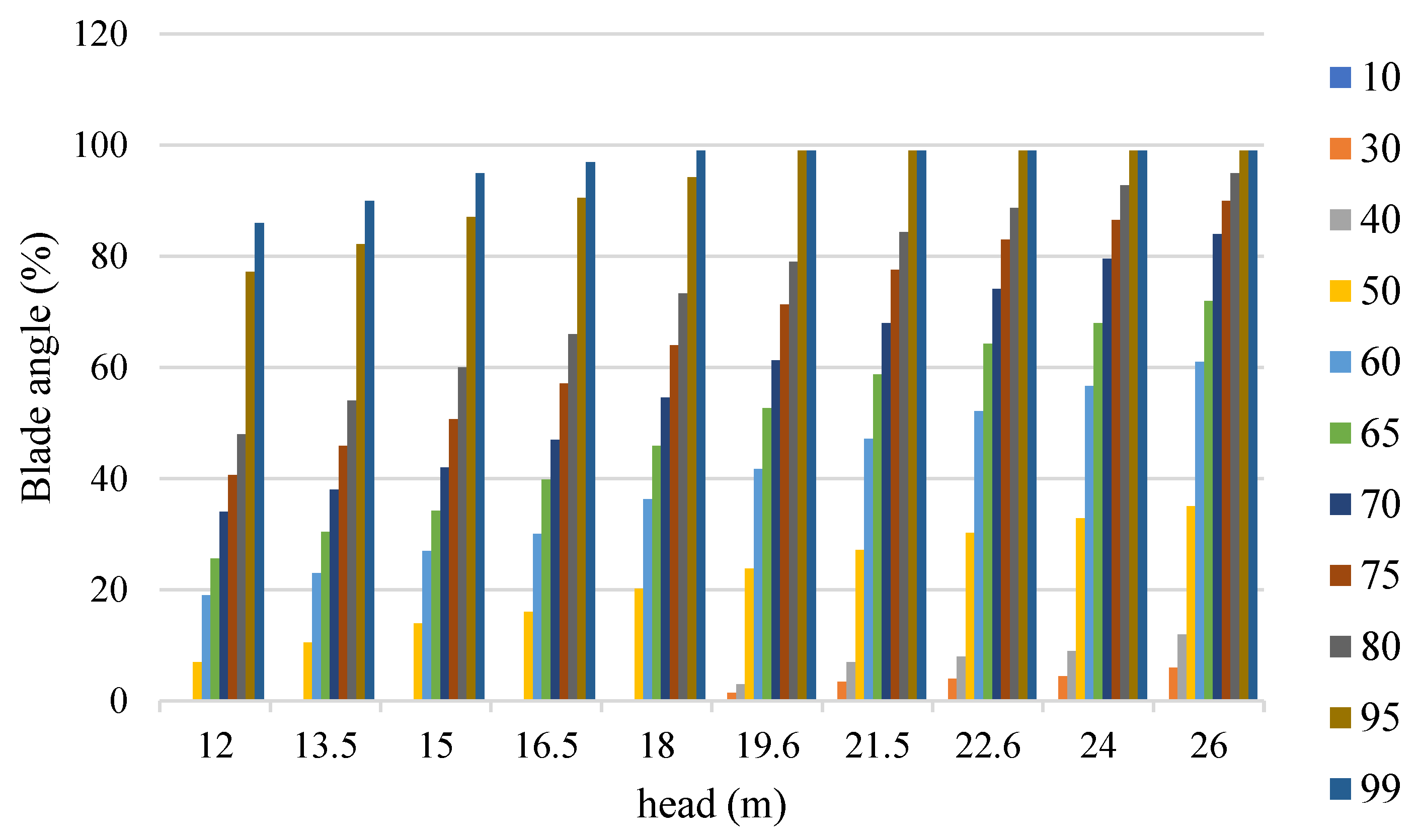
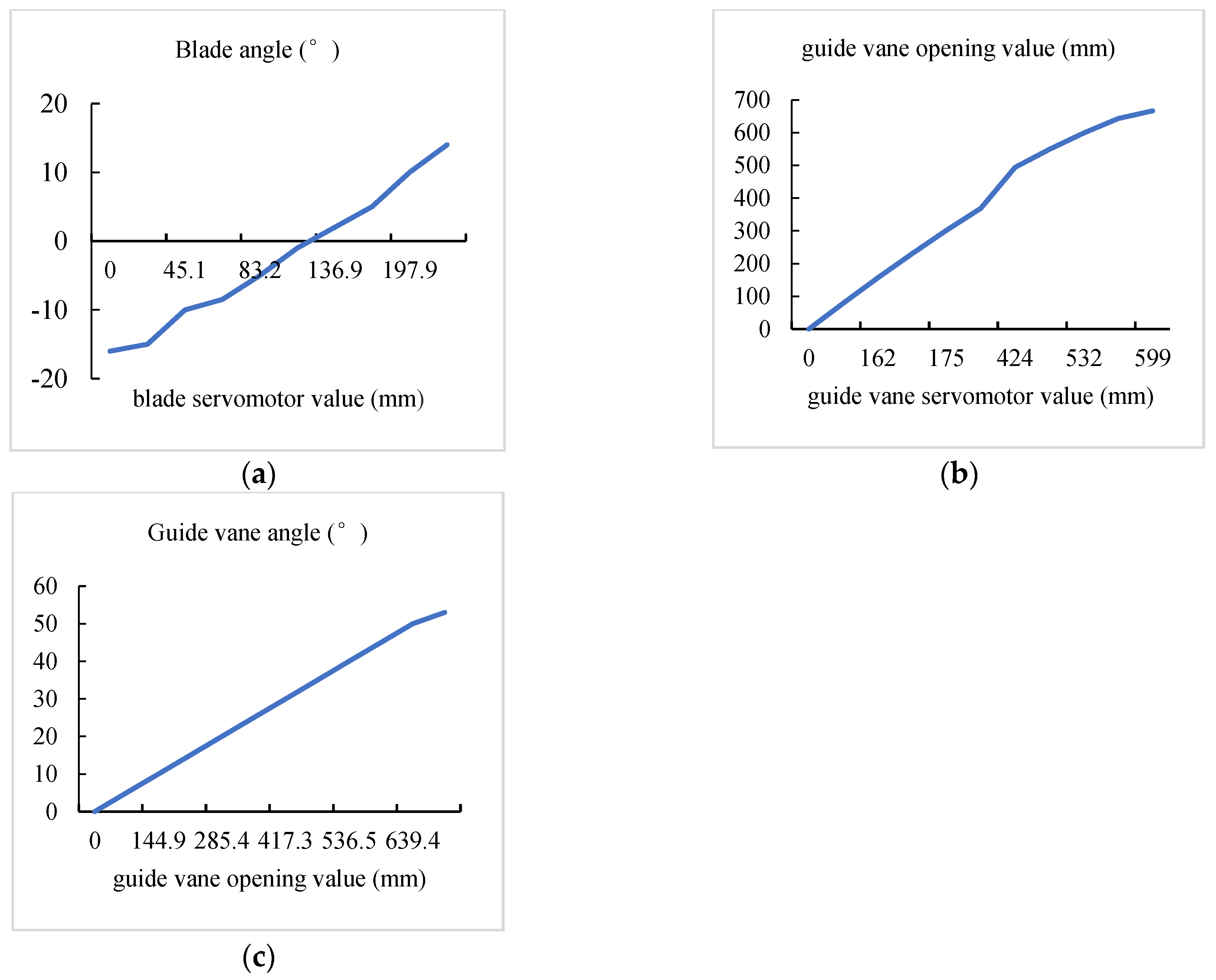
This paper takes a Kaplan HPP in China as a study case. The basic parameters of the hydropower station are listed in Table A2. There is a cam relationship between the guide vane and the blade of the Kaplan hydropower unit, which means that the blade will change with the guide vane in a certain way during regulation process. In addition, there is also a relationship between the guide vane servomotor value and the guide vane opening value. Thus, the guide vane opening value and the guide vane angle, the blade servomotor value, and the blade angle is not linear. As such, the simulation model should be established according to the real data of HPP. Figure 9 shows the cam relationship established in this paper on the basis of the studied HPP. There are 11 blade angle values in each head, and they vary under a certain guide vane opening value series, which are defined in different colors in Figure 9 and listed in Table A3. Figure A2 illustrates the relationships between blade servomotor value and blade angle, guide vane servomotor value and guide vane opening value, and guide vane opening value and guide vane angle.
For the turbine model, considering the point of the model characteristic curve of the studied hydropower plant and performing interpolation fitting calculation, the relationship among the unitary flow rate, the unitary speed, and the guide vane opening is obtained. Also, the relationships among the unitary torque, the unitary speed, and the guide vane opening at different water heads and at different blade angles are obtained. Figure 10 illustrates the relationship between the unit flow rate and the unit speed and the opening degree of the guide vane. Figure 11 shows the relationship between the unit torque and the unit rotation speed and the vane opening degree when the blade angle is 14 degrees. In these two figures, there are 17 unit discharge values in each guide vane angle, and they vary under certain unit rotation speed series, which are defined in different colors and listed in Table A4. The simulation model determines the unit moment and the unit flow rate of the unit under different parameters by fitting the relationship.
3. Model Validation
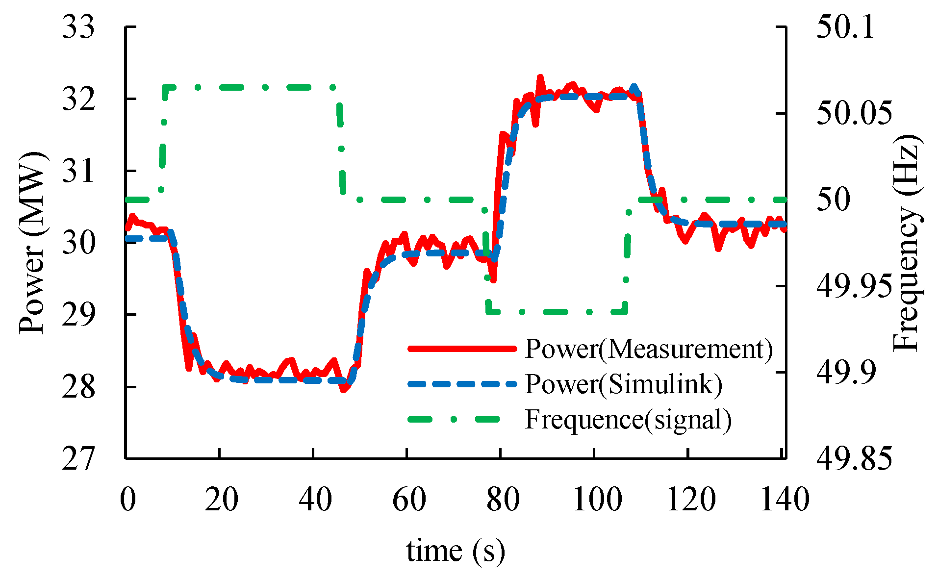
In this chapter, we verify the accuracy of the hydroelectric unit model. To achieve this, the improved frequency dead zone is adopted. However, the feed-forward control is not used. In this experiment, the parameters of the simulation model are set according to the actual parameters of the hydropower units. The specific parameters are listed in case 1 of Table A5, and the hardware prototype for the experiment is shown in Figure A3. When the step signal acts on ±0.065 Hz and ±0.055 Hz, respectively, the results of the active power change obtained by the simulation model are compared with those obtained by the experiment measurement. By comparing the fitting degree of the simulated active power variation curve with the measured active power variation curve under the same step disturbance, it is possible to determine whether the established hydropower unit model truly reflects the actual hydropower unit. Figure 12 shows the active power variation curves obtained by field measurement and model simulation under the action of step signals at ±0.065 Hz. Figure 13 displays the curve of active power variation obtained by field measurement and model simulation at ±0.055 Hz.
Comparing the active power simulation results and the experimental measurement results, it is observable that the simulated active power variation curve can be better matched with the actual active power variation curve. This confirms that the hydropower model established in this paper can better reflect the actual hydropower unit. As such, the impact of this model on the frequency dead zone can be studied in depth.
4. Results
4.1. Analysis of Dynamic Response
In this section, two sets of simulation experiments conducted by the unit simulation model are taken as examples to analyze the effects of different types of frequency dead zones and the active power output of the unit after the introduction of feed-forward control. The parameters of the simulation model are set according to case 2 of Table A5. In the first group of experiments, the common frequency dead zone, the enhanced frequency dead zone, and the improved frequency dead zone are separately acted on the simulation model. By calculating the results of the guide vane opening, the blade angle, and the active power change under step disturbance, the dynamic process and influence mechanism of PFC under the action of three frequency dead zones can be analyzed. In the second group, a feed-forward control is added when the enhanced frequency dead zone and the improved frequency dead zone act. By comparing the guide vane opening, the blade angle, and the active power of the common frequency dead zone, the enhanced frequency dead zone combined with feed-forward control, the improved dead zone combined with feed-forward control, and the dynamic response process of PFC is analyzed.
4.1.1. Analysis of PFC with Three Dead Zones
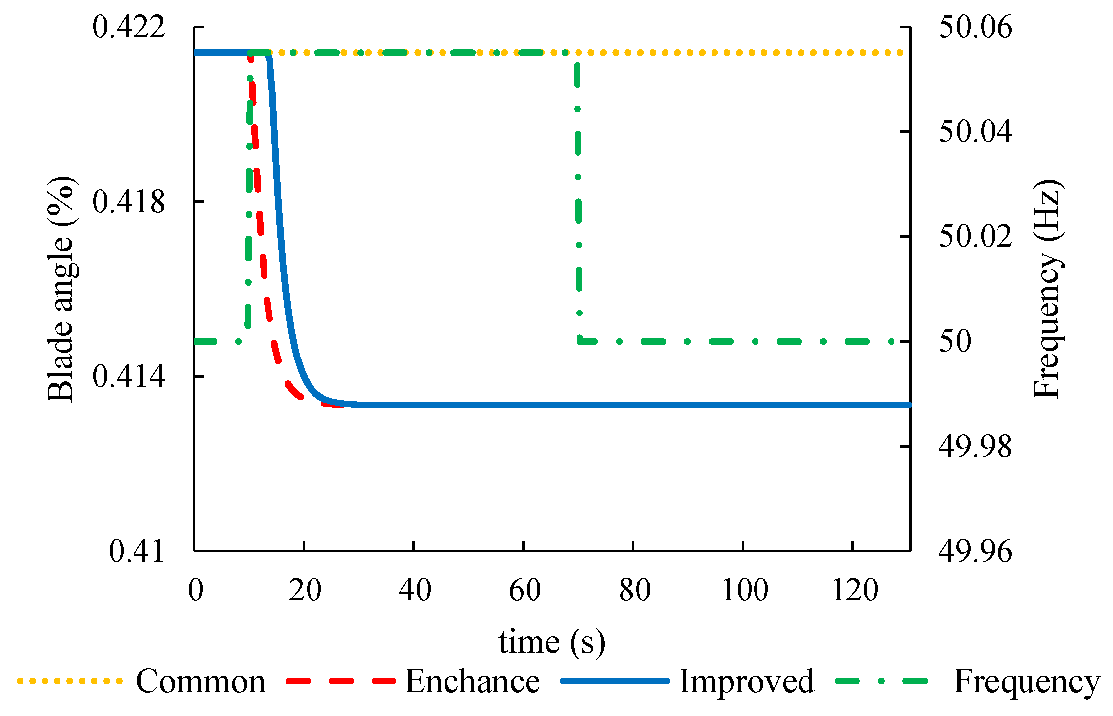
The common, enhanced, and improved frequency dead zones are respectively applied to the simulation model. Figure 14 illustrates the dynamic response process of the guide vane opening calculated, while Figure 15 shows the dynamic response process of the blade angle. Figure 16 indicates the dynamic response process of the active power.
From the simulation results of the PFC dynamic response under three different dead zones, it is clear that when the frequency changes from 50 Hz to 50.055 Hz in step, the common frequency dead zone eliminates the regulation movement. Also, when the enhanced frequency dead zone and the improved frequency dead zone are adopted, the guide vane opening and the blade opening are increased compared with the common frequency dead zone. In addition, the variation of active power is significantly increased. By comparing the simulation results of the enhanced frequency dead zone with the improved frequency dead zone, the servo system regulates more quickly than the improved frequency dead zone when the enhanced frequency dead zone is applied. Additionally, if the unit runs in the frequency dead zone for a long time, frequent actions and resets occur in the PFC. Moreover, large regulation actions in the servo system of the unit accelerate the wear and tear of the unit and consequently affect the life of the regulation system. However, by adopting the improved frequency dead zone, the frequency difference calculated by this dead zone is gradually increased. As a result, the action of the servo system is gradually increased. Also, when the system is disturbed by small frequency differences frequently, the servo system will not frequently take large regulation. This will reduce the unit wear and tear.
When the system frequency is stepped back from 50.055 Hz to 50 Hz, and by action of the three dead zones, the regulation system will not act. Consequently, the active power output will not return to the initial steady state value. This is due to the fact that in the power mode, when the step signal falls down, the frequency difference calculated by the frequency dead zone is opposite to the given power value symbol. Furthermore, it is canceled before the power dead zone is calculated, resulting in the power dead zone filtering when the power dead zone is less than the set value of the power dead zone. In this case, the servo system does not react and cannot return to the target power.
4.1.2. Analysis of PFC under Common Frequency Dead Zone, Enhanced Frequency Dead Zone with Feed-Forward Control, and Improved Frequency Dead Zone with Feed-Forward Control
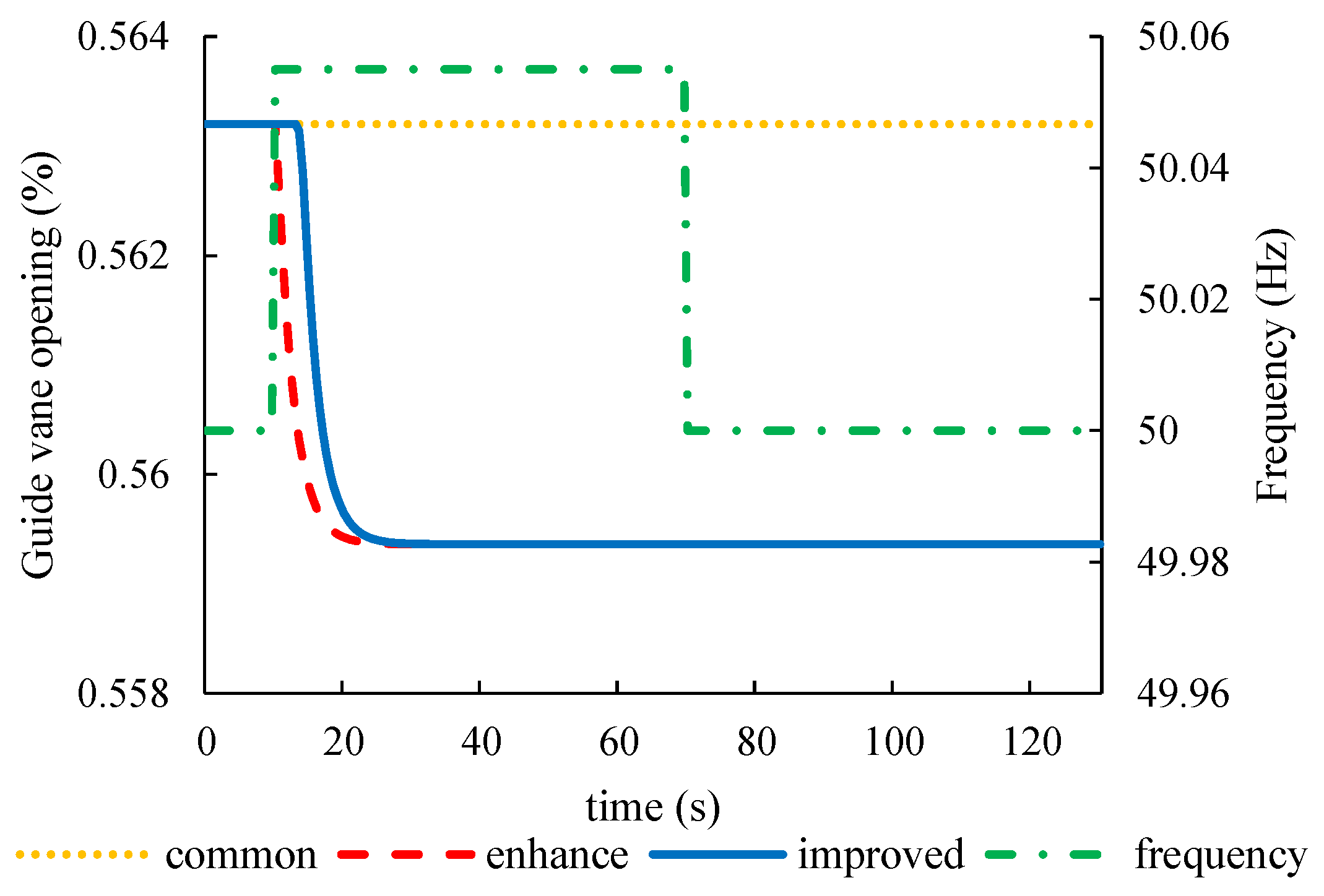
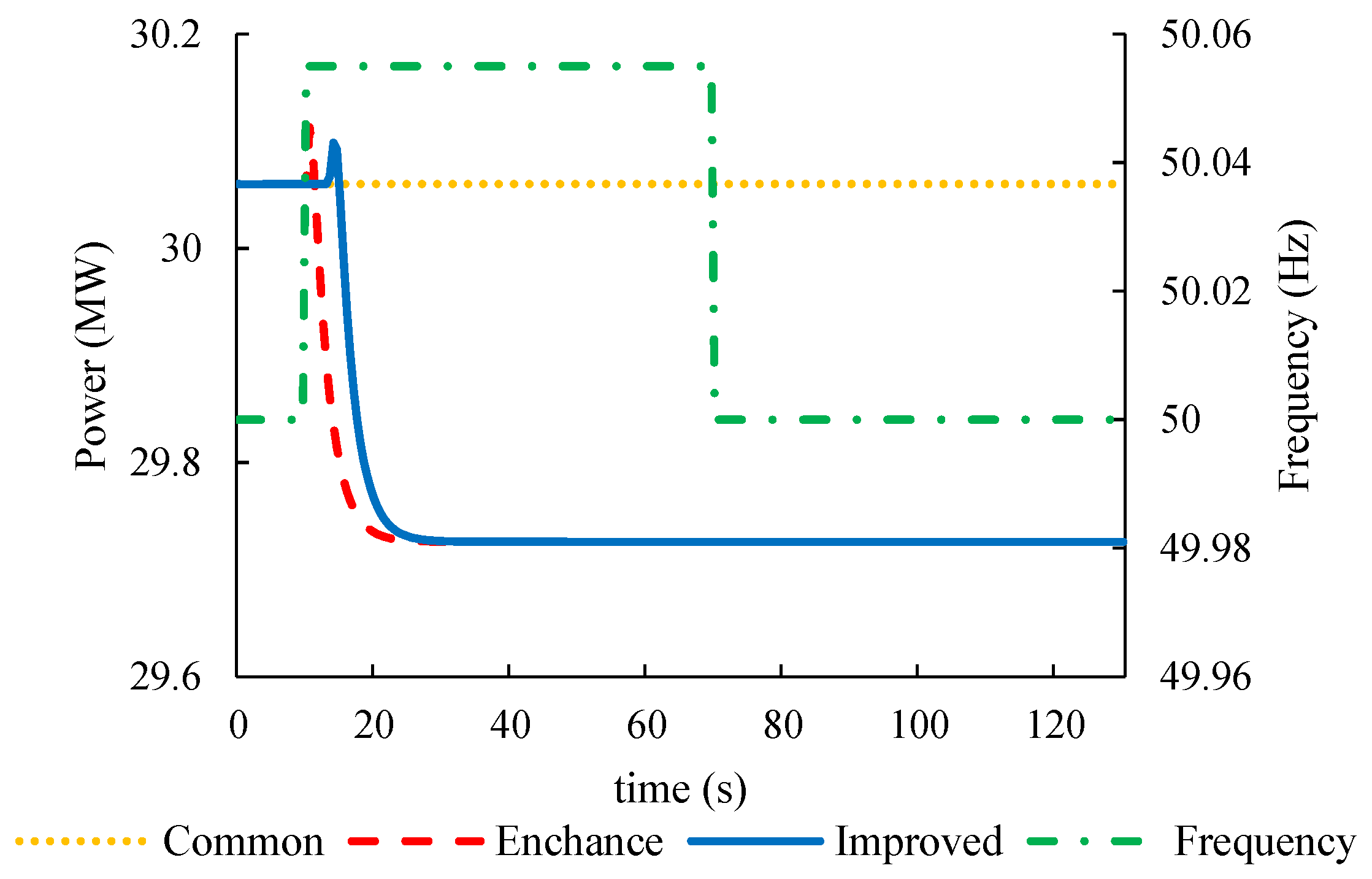
To solve the problem discussed in Section 4.1.1 (that PFC cannot return to the target power), the feed-forward control is introduced when the enhanced frequency dead zone and the improved frequency dead zone are applied in simulation experiments. Figure 17 illustrates the dynamic response process of the guide vane opening calculations. Meanwhile, Figure 18 shows the dynamic response process of the blade angle, and Figure 19 indicates the dynamic response process of active power.
After the application of the feed-forward control into the enhanced frequency dead zone and the improved frequency dead zone, the feed-forward control section calculates the current steady-state output opening Ypid as per the current frequency difference and the given power value. This guarantees that the power can be regulated back to the target power when the system frequency step falls back to 50 Hz. At the same time, as a result of the combined action of feed-forward control and PID, the regulation amount of the whole regulation process is increased, while the output of active power is increased. In the case of step disturbance, the regulating quantity and the active power output of the servo system are significantly larger than those of the enhanced and the improved frequency dead zones adopted alone, which can effectively improve the IQE.
4.2. Trade-Off and Assessment
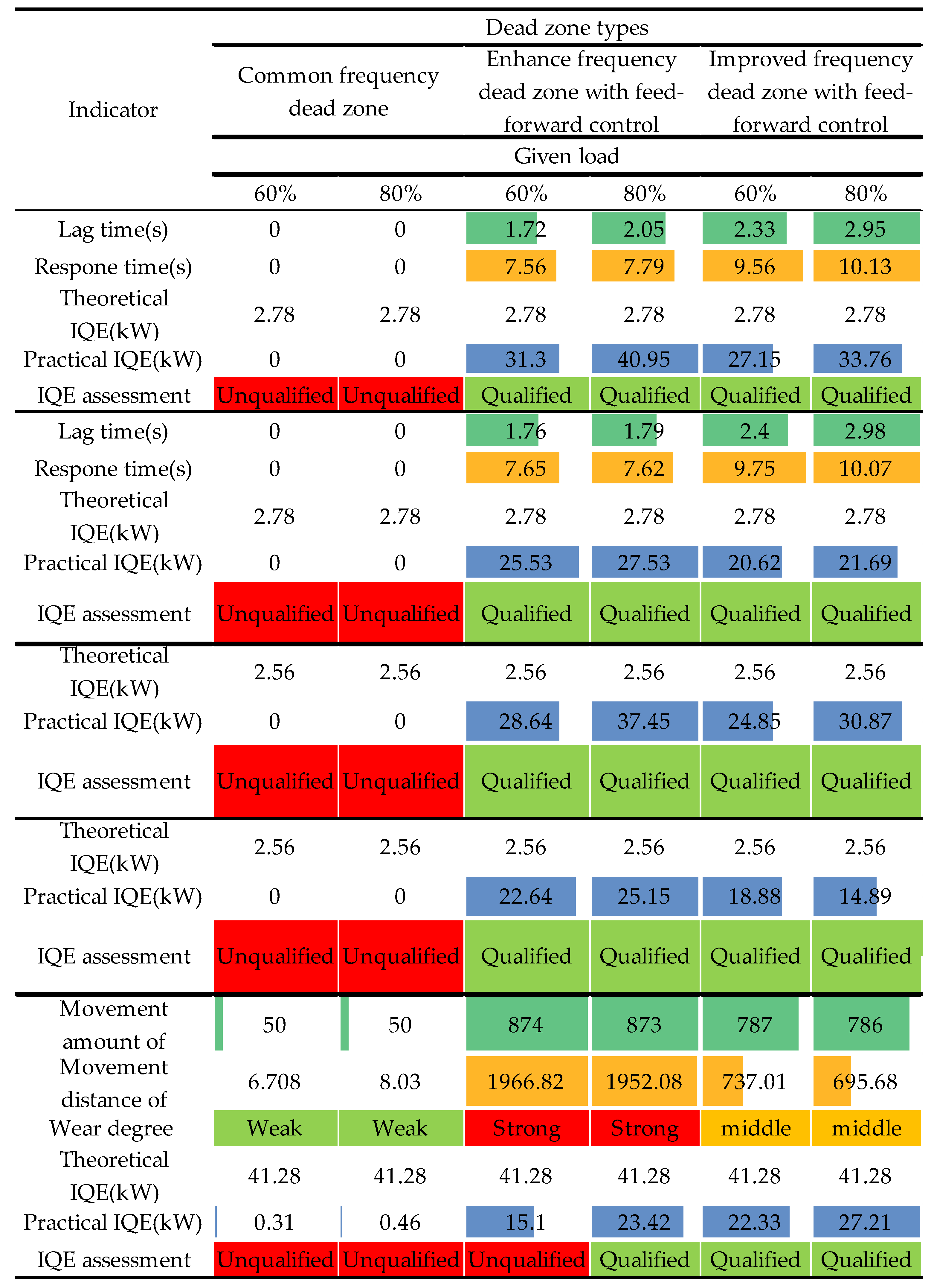
Drawing from the discussion under Section 4.1, the common frequency dead zone, the enhanced frequency dead zone combined with feed-forward control, and the improved frequency dead zone combined with feed-forward control are applied to the regulating system, respectively, in this section. After that, under the step disturbance and the ramp disturbance, the IQE and the regulating speed of the three dead zones are simulated and calculated. In addition, the simulation is carried out from the IQE and wear and tear of the servo system under the disturbance of 7000 s real frequency. Figure 20 summarizes the simulation results, while Table A5 shows the simulation model parameters set in accordance with case 2.
From Figure 20, under the disturbance of step signal and ramp signal, the common frequency dead zone has no action. As such, the lag time and the response time are zero, while the practical IQE is also zero. This means that when the loads are the same, because the frequency difference obtained by the enhanced frequency dead zone is larger than that of the improved frequency dead zone in the initial regulation, the amount of regulation movements of the enhanced frequency dead zone with feed-forward control will be larger than that of the improved frequency dead zone with feed-forward control under the disturbance of step signal and ramp signal. Therefore, when the enhanced frequency dead zone with feed-forward control is applied to the model, the lag time and the response time reflecting the regulation speed will be smaller than those of the improved frequency dead zone with feed-forward control. However, when these two kinds of dead zones are adopted, both the lag time and the response time will meet the requirement of the regulation speed in the PFC. That is, the lag time is less than 3.0 s and the response time is less than 11.0 s when the load is 80% under step disturbance. The practical IQE of the enhanced frequency dead zone with feed-forward control will also be larger than that of the improved frequency dead zone with feed-forward control. In brief, it is observable that according to the evaluation of IQE by the power grid, after adopting feed-forward control, the practical IQE of two frequency dead zones will be more than 50% of the theoretical IQE. This means that the integral electric quantity is qualified.
When the real frequency is applied, the frequency difference of the common frequency dead zone is small, and the movements amount along with the total distance of servomotor are the least in 7000 s. Thus, the wear and tear of the servo system are the smallest. However, in 7000 s with 80% load, the practical IQE is found to be 0.46, which is only 1.1% of the theoretical IQE. This means that the IQE is not qualified. For the enhanced frequency dead zone with feed-forward control, the frequency difference used to calculate is regarded to be larger than the improved frequency dead zone with feed-forward control in the regulation process. In this case, the amount and the distance of the servomotor movements are larger than the improved frequency dead zone with feed-forward control. Also, the wear performance is the worst. From the IQE of the two dead zones in 7000 s real frequency, when the same load is given, the practical IQE of the improved frequency dead zone with feed-forward control will be larger than that of the enhanced frequency dead zone with feed-forward control, which is contrary to the step signal and the ramp signal. Moreover, although the practical IQE of both is greater than 50% of the theoretical IQE when the load is given to 80%, the practical IQE of the enhanced frequency dead zone is still less than 50% of the theoretical IQE when the given load is 60%. Thus, the integral electric quantity of the unit is not qualified. At the same time, according to the comparison of the real frequency results, the improved frequency dead zone with feed-forward control is regarded to be better than the other two dead zones.
5. Conclusions
This paper proposed an improved frequency dead zone model with feed-forward control to reduce the wear of enhanced frequency dead zone model as well as to improve the problem of insufficient active power output and unqualified integral quantity of electricity of hydropower units during primary frequency control. Firstly, an improved frequency dead zone was proposed on the basis of the common frequency dead zone and the enhanced frequency dead-zone. In addition, the method of feed-forward control applied to primary frequency control was introduced. After that, the model of hydropower plants with Kaplan units was established by applying MATLAB/Simulink based on a real hydropower plant in China. Also, the simulation model was verified by the experimental results. Through the simulation, the dynamic processes of primary frequency control were compared and analyzed under the implementations of the common frequency dead zone, the enhanced frequency dead zone, and the improved frequency dead zone. Finally, the simulation results of the enhanced frequency dead zone and improved frequency dead zone combined with the feed-forward control and the common frequency dead zone were summarized in Figure 20.
The following conclusions are drawn:
Compared with the common frequency dead zone, the improved dead zone could effectively increase the movement of the servo system in the primary frequency control process. It could also lead to less wear and tear of hydropower units in contrast to the enhanced frequency dead zone. The feed-forward control was applied to ascertain that the unit could achieve the target power value (and increase the output of active power). When the feed-forward control and the improved frequency dead zone were both activated, the IQE was found to be larger than that of the ordinary type and the enhanced type under the actual grid frequency disturbances. Although the IQE of the improved dead zone was slightly smaller than that of the enhanced frequency dead zone under the step disturbance and the ramp disturbance, it was much larger than the IQE of the target value of the power grid, which could still ensure the qualification of IQE and the economic benefit of the HPP. At the same time, the proposed dead zone could effectively relieve the wear and tear problem of the enhanced frequency dead zone and consequently reduce the maintenance cost of the HPP. In particular, the improved frequency dead zone proposed in this paper was successfully implemented in practical HPPs in China.
In this paper, the HPP with a Kaplan turbine was the main study objective. The head of the Kaplan units is usually low, and the output of active power is generally small. For future works, therefore, it would be meaningful to further investigate the performances for HPPs or pumped storage plants with complex waterway systems and Francis turbines with high water head and large capacity.
Author Contributions
Conceptualization, J.Y. and Y.C.; Data curation, H.A. and Y.C.; Formal analysis, H.A. and W.Y.; Funding acquisition, W.Y.; Investigation, H.A.; Methodology, H.A. and W.Y.; Resources, J.Y., W.Y., Y.C. and Y.P.; Software, H.A.; Supervision, J.Y. and Y.C.; Visualization, H.A. and Y.P.; Writing—original draft, H.A.; Writing—review & editing, J.Y. and W.Y.
Funding
The authors are thankful for the support from the National Natural Science Foundation of China (No.51809197, No.51879200, No.51839008), the National Key Research and Development Program of China (No.2017YFB0903700).
Conflicts of Interest
The authors declare no conflict of interest.
Appendix A

Table A1.
Steady Ypid values of feed-forward control calculating at different water heads and loads.
Table A1.
Steady Ypid values of feed-forward control calculating at different water heads and loads.
| Head/m | Ypid | ||||||||||
|---|---|---|---|---|---|---|---|---|---|---|---|
| Load (%) | |||||||||||
| 0 | 10 | 20 | 30 | 40 | 50 | 60 | 70 | 80 | 90 | 100 | |
| 12.9 | 0.13 | 0.34 | 0.60 | 0.70 | 0.84 | 0.90 | 0.98 | 1.00 | 1.00 | 1.00 | 1.00 |
| 14 | 0.12 | 0.29 | 0.55 | 0.65 | 0.76 | 0.85 | 0.94 | 1.00 | 1.00 | 1.00 | 1.00 |
| 16 | 0.11 | 0.24 | 0.48 | 0.58 | 0.65 | 0.74 | 0.82 | 0.90 | 0.99 | 1.00 | 1.00 |
| 18 | 0.10 | 0.21 | 0.42 | 0.50 | 0.57 | 0.64 | 0.71 | 0.78 | 0.85 | 0.93 | 1.00 |
| 20.7 | 0.09 | 0.18 | 0.31 | 0.44 | 0.50 | 0.55 | 0.61 | 0.67 | 0.72 | 0.77 | 0.84 |
| 22.1 | 0.08 | 0.16 | 0.27 | 0.41 | 0.46 | 0.50 | 0.56 | 0.61 | 0.67 | 0.70 | 0.75 |
| 23 | 0.08 | 0.16 | 0.26 | 0.40 | 0.45 | 0.49 | 0.54 | 0.59 | 0.64 | 0.68 | 0.72 |
| 25.29 | 0.08 | 0.15 | 0.23 | 0.34 | 0.42 | 0.46 | 0.49 | 0.53 | 0.57 | 0.62 | 0.65 |
Figure A1.
Ypid fitting of feed-forward control. The 11 values under each head represent the load from 0% to 100%.
Figure A1.
Ypid fitting of feed-forward control. The 11 values under each head represent the load from 0% to 100%.

Table A2.
Basic parameters of experimental HHP.
| Parameter | Value |
|---|---|
| Rated output power (MW) | 50.1 |
| Rated discharge (m3/s) | 270.4 |
| Rated head (m) | 20.7 |
| Minimum head (m) | 12.9 |
| Maximum head (m) | 25.29 |
| Rated speed (rpm) | 115.4 |
Table A3.
Vane opening value series of cam relationship.
| Vane Opening Values (%) | |||||||||
|---|---|---|---|---|---|---|---|---|---|
| 30 | 40 | 50 | 60 | 65 | 70 | 75 | 80 | 95 | 99 |
Table A4.
The unit rotation speed series.
| Unit Rotation Speed (m/s) | ||||||||||||||||
|---|---|---|---|---|---|---|---|---|---|---|---|---|---|---|---|---|
| 0 | 30 | 60 | 90 | 110 | 120 | 125.18 | 136.62 | 140.6 | 147.11 | 153.55 | 160 | 186.35 | 200 | 250 | 300 | 360 |
Table A5.
Parameter setting of simulation experiment.
| Parameter | Case1 | Case2 |
|---|---|---|
| ep | 0.03 | 0.03 |
| Kp | 0.1 | 0.1 |
| Kd | 0 | 0 |
| Ki, Kip | 0.15, 0 | 0.15, 0.4 |
| T1v | 0.16 | 0.16 |
| Ef | 0.05 | 0.05 |
| Ep | 0.005 | 0.03 |
| Ty | 8.33 | 8.33 |
| Tw | 1.7 | 1.7 |
| Ta | 8.76 | 8.76 |
| Initial Head (m) | 22.1 | 22.1 |
| Given load (%) | 60% | 60% & 80% |
| Step signal | ±0.055 Hz & ±0.065 Hz | ±0.055 Hz |
Figure A2.
The relationship between blade servomotor value and blade angle (a), guide vane servomotor value and guide vane opening value (b), guide vane opening value and guide vane angle (c).
Figure A2.
The relationship between blade servomotor value and blade angle (a), guide vane servomotor value and guide vane opening value (b), guide vane opening value and guide vane angle (c).

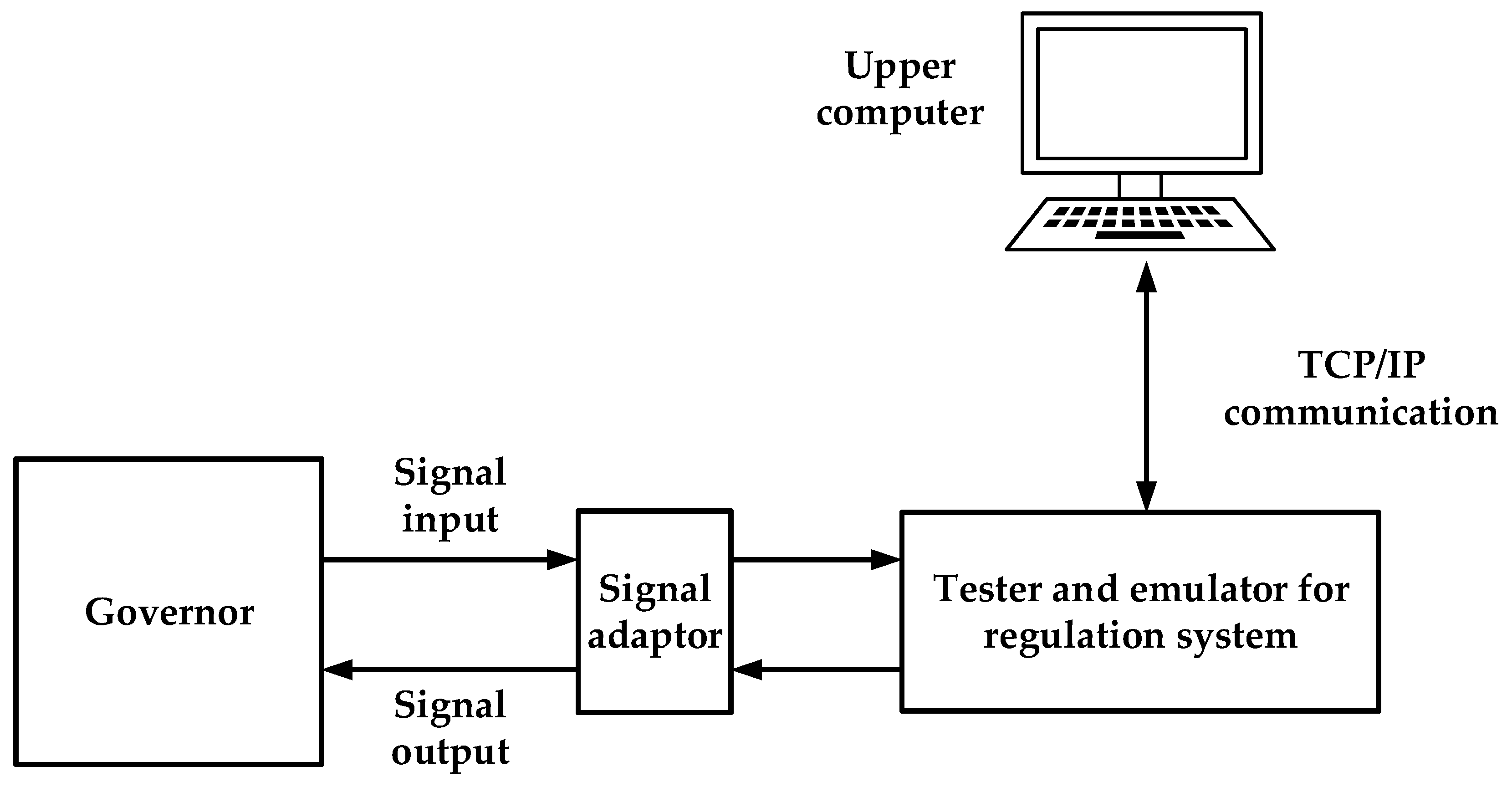
Figure A3.
The hardware prototype for actual experiment. Through the instructions from Upper computer, Tester and emulator for regulation system sends frequency step signals to Governor and acquires power outputs measured by Governor, then these figures are saved in the Upper computer and displayed on the screen.

References
- Mitchell, C. Momentum is increasing towards a flexible electricity system based on renewables. Nat. Energy 2016, 1, 15030. [Google Scholar] [CrossRef]
- Brouwer, A.S.; van den Broek, M.; Seebregts, A.; Faaij, A. Operational flexibility and economics of power plants in future low-carbon power systems. Appl. Energy 2015, 156, 107–128. [Google Scholar] [CrossRef] [Green Version]
- Storli, P.; Nielsen, T. Dynamic load on a Francis turbine runner from simulations based on measurements. IOP Conf. Ser. Earth Environ. Sci. 2014, 22, 032056. [Google Scholar] [CrossRef]
- Doujak, E. Effects of increased solar and wind energy on hydro plant operation. Hydro Rev. Worldw. 2014, 2, 28–31. [Google Scholar]
- Ming, B.; Liu, P.; Guo, S.; Zhang, X.; Feng, M.; Wang, X. Optimizing utility-scale photovoltaic power generation for integration into a hydropower reservoir by incorporating long-and short-term operational decisions. Appl. Energy 2017, 204, 432–445. [Google Scholar] [CrossRef]
- Wang, W.; Li, C.; Liao, X.; Qin, H. Study on unit commitment problem considering pumped storage and renewable energy via a novel binary artificial sheep algorithm. Appl. Energy 2017, 187, 612–626. [Google Scholar] [CrossRef]
- Chang, M.K.; Eichman, J.D.; Mueller, F.; Samuelsen, S. Buffering intermittent renewable power with hydroelectric generation: A case study in California. Appl. Energy 2013, 112, 1–11. [Google Scholar] [CrossRef]
- Ma, T.; Yang, H.; Lu, L.; Peng, J. Pumped storage-based standalone photovoltaic power generation system: Modeling and techno-economic optimization. Appl. Energy 2015, 137, 649–659. [Google Scholar] [CrossRef]
- Yang, W.; Norrlund, P.; Saarinen, L.; Witt, A.; Smith, B.; Yang, J.; Lundin, U. Burden on hydropower units for short-term balancing of renewable power systems. Nat. Commun. 2018, 9, 2633. [Google Scholar] [CrossRef]
- Cebeci, M.E.; Karaagaç, U.; Tör, O.B.; Ertas, A. The effects of hydro power plants’governor settings on the stability of turkish power system frequency. In Proceedings of the 5th International Conference on Electrical and Electronics Engineering, Bursa, Turkey, 5–9 December 2007. [Google Scholar]
- Ela, E.; Tuohy, A.; Milligan, M.; Kirby, B.; Brooks, D. Alternative Approaches for Incentivizing the Frequency Responsive Reserve Ancillary Service. Electr. J. 2012, 25, 88–102. [Google Scholar] [CrossRef] [Green Version]
- Ela, E.; Gevorgian, V.; Tuohy, A.; Kirby, B.; Milligan, M.; O’Malley, M. Market Designs for the Primary Frequency Response Ancillary Service—Part I: Motivation and Design. IEEE Trans. Power Syst. 2014, 29, 421–431. [Google Scholar] [CrossRef]
- Raineri, R.; Ríos, S.; Schiele, D. Technical and economic aspects of ancillary services markets in the electric power industry: An international comparison. Energy Policy 2006, 34, 1540–1555. [Google Scholar] [CrossRef]
- Rebours, Y.G.; Kirschen, D.S.; Trotignon, M.; Rossignol, S. A survey of frequency and voltage control ancillary services—Part II: Economic features. IEEE Trans. Power Syst. 2007, 22, 358–366. [Google Scholar] [CrossRef]
- Rebours, Y.G.; Kirschen, D.S.; Trotignon, M. A Survey of Frequency and Voltage Control Ancillary Services-Part I: Technical Features. IEEE Trans. Power Syst. 2007, 22, 350–357. [Google Scholar] [CrossRef]
- Zhang, S.; Andrews-Speed, P.; Li, S. To what extent will China’s ongoing electricity market reforms assist the integration of renewable energy? Energy Policy 2018, 114, 165–172. [Google Scholar] [CrossRef]
- Ming, Z.; Ximei, L.; Lilin, P. The ancillary services in China: An overview and key issues. Renew. Sustain. Energy Rev. 2014, 36, 83–90. [Google Scholar] [CrossRef]
- Pollitt, M.; Yang, C.-H.; Chen, H. Reforming the Chinese Electricity Supply Sector: Lessons from International Experience; Cambridge Working Papers in Economics; University of Cambridge: Cambridge, UK, 2017. [Google Scholar]
- Yang, W.; Yang, J.; Guo, W.; Norrlund, P. Response time for primary frequency control of hydroelectric generating unit. Int. J. Electr. Power Energy Syst. 2016, 74, 16–24. [Google Scholar] [CrossRef] [Green Version]
- Wei, S. Analysis and Simulation on the Primary Frequency Regulation and Isolated Grid Operation Characteristics of Hydraulic Turbine Regulating Systems. Hydropower Autom. Dam Monit. 2009, 33, 27–33. (In Chinese) [Google Scholar]
- Jones, D.I.; Mansoor, S.P.; Aris, F.C.; Jones, G.R.; Bradley, D.A.; King, D.J. A standard method for specifying the response of hydroelectric plant in frequency-control mode. Electr. Power Syst. Res. 2004, 68, 19–32. [Google Scholar] [CrossRef]
- Andrade, J.; Júnior, E.; Ribeiro, L. Using genetic algorithm to define the governor parameters of a hydraulic turbine. In Proceedings of the 25th IAHR Symposium on Hydraulic Machinery and Systems, Timisoara, Romania, 20–24 September 2010. [Google Scholar]
- Li, C.S.; Zhou, J.Z. Parameters identification of hydraulic turbine governing system using improved gravitational search algorithm. Energy Convers. Manag. 2011, 52, 374–381. [Google Scholar] [CrossRef]
- Yang, W.; Norrlund, P.; Saarinen, L.; Yang, J.; Guo, W.; Zeng, W. Wear and tear on hydro power turbines–Influence from primary frequency control. Renew. Energy 2016, 87, 88–95. [Google Scholar] [CrossRef]
- Yang, W.; Norrlund, P.; Saarinen, L.; Yang, J.; Zeng, W.; Lundin, U. Wear reduction for hydro power turbines considering frequency quality of power systems: A study on controller filters. IEEE Trans. Power Syst. 2016, 32, 1191–1201. [Google Scholar]
- Ukonsaari, J. Wear, fraction and synthetic esters in a boundary lubricated journal bearing. Tribol. Int. 2003, 36, 821–826. [Google Scholar] [CrossRef]
- Gawarkiewicz, R.; Wasilczuk, M. Wear measurements of self-lubricating bearing materials in small oscillatory movement. Wear 2007, 263, 458–462. [Google Scholar] [CrossRef]
- Simmons, G.F. Journal Bearing Design, Lubrication and Operation for Enhanced Performance; University of Technology: Luleå, Sweden, 2013. [Google Scholar]
- Chirag, T.; Bhupendra, G.; Michel, C. Effect of transients on Francis turbine runner life: A review. J. Hydraul. Res. 2013, 51, 12. [Google Scholar]
- Huth, H. Fatigue Design of Hydraulic Turbine Runners; Department of Engineering Design & Materials: Trondheim, Norway, 2005. [Google Scholar]
- Gagnon, M.; Tahan, S.A.; Bocher, P. Impact of startup scheme on Francis runner life expectancy. IOP Conf. Ser. Earth Environ. Sci. 2010, 12, 012107. [Google Scholar] [CrossRef] [Green Version]
- Wurm, E. Consequences of Primary Control to the Residual Service Life of Kaplan Runners. In Proceedings of the Russia Power 2013 & Hydro vision Russia, Moscow, Russia, 4–6 March 2013. [Google Scholar]
- Nilsson, O.; Sjelvgren, D. Hydro unit start-up costs and their impact on the short term scheduling strategies of Swedish power producers. IEEE Trans. Power Syst. 1997, 12, 38–44. [Google Scholar] [CrossRef]
- Bakken, B.H.; Bjorkvoll, T. Hydropower unit start-up costs. In Proceedings of the 2002 IEEE Power Engineering Society Summer Meeting, Chicago, IL USA, 21–25 July 2002; pp. 1522–1527. [Google Scholar]
- Nilsson, O.; Sjelvgren, D. Variable splitting applied to modelling of start-up costs in short term hydro generation scheduling. IEEE Trans. Power Syst. 1997, 12, 770–775. [Google Scholar] [CrossRef]
- Guisandez, I.; Perez-Díaz, J.I.; Wilhelmi, J.R. Assessment of the economic impact of environmental constraints on annual hydropower plant operation. Energy Policy 2013, 61, 1332–1343. [Google Scholar] [CrossRef]
- Aggidis, G.A.; Luchinskaya, E.; Rothschild, R.; Howard, D. The costs of small-scale hydro power production: Impact on the development of existing potential. Renew. Energy 2010, 35, 2632–2638. [Google Scholar] [CrossRef]
- Huang, S.R.; Chang, P.L.; Hwang, Y.W.; Ma, Y.H. Evaluating the productivity and financial feasibility of a vertical-axis micro-hydro energy generation project using operation simulations. Renew. Energy 2014, 66, 241–250. [Google Scholar] [CrossRef]
- Bean, N.G.; O’Reilly, M.M.; Sargison, J.E. A Stochastic Fluid Flow Model of the Operation and Maintenance of Power Generation Systems. IEEE Trans. Power Syst. 2010, 25, 1361–1374. [Google Scholar] [CrossRef]
- Ieee BE. IEEE Guide for the Application of Turbine Governing Systems for Hydro Electric Generating Units; IEEE Std. 1207–2011 (Revision to IEEE Std. 1207-2004); IEEE: New York, NY, USA, 2011; pp. 1–131. [Google Scholar]
- Li, X.; Xu, G.; Huang, Q. Analysis of dynamic response of enhanced primary frequency regulation of hydropower units. Water Resour. Power 2016, 34, 152–155. (In Chinese) [Google Scholar]
- Khodabakhshian, A.; Hooshmand, R. A new PID controller design for automatic generation control of hydro power systems. Int. J. Electr. Power Energy Syst. 2010, 32, 375–382. [Google Scholar] [CrossRef]
- Kishor, N.; Saini, R.P.; Singh, S.P. A review on hydropower plant models and control. Renew. Sustain. Energy Rev. 2007, 11, 776–796. [Google Scholar] [CrossRef]
- China Electricity Council, The grid operation code. C.E. Council, DL/T 1040–2007; China Electricity Council: Beijing, China, 2007. [Google Scholar]
Figure 1.
7000 s real frequency.
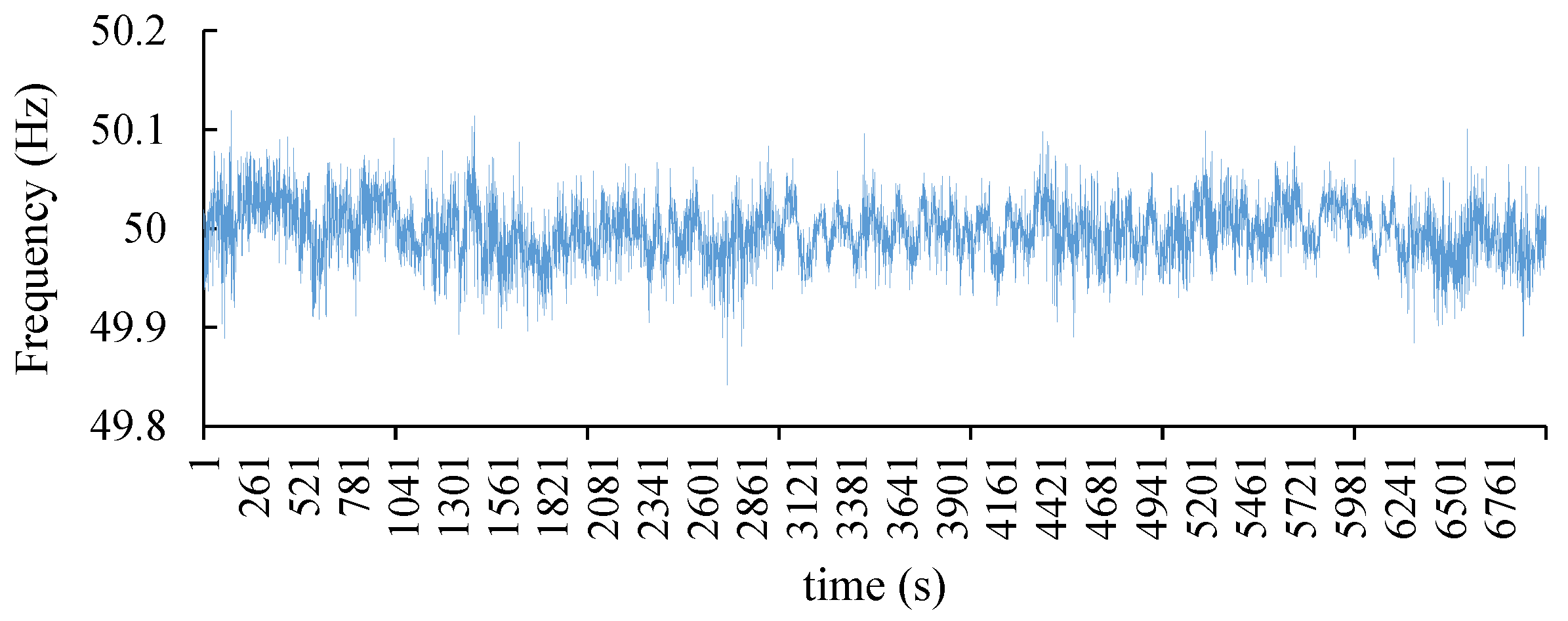
Figure 2.
Measured frequency fluctuation statistics of power grid in 7000 s.
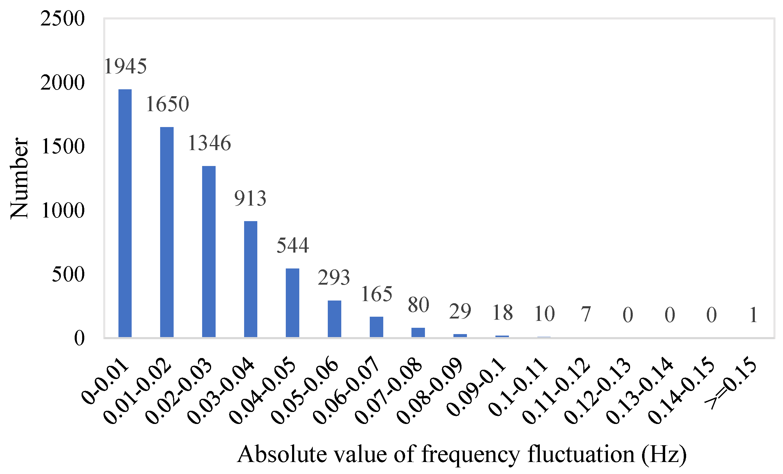
Figure 3.
The common frequency dead zone.
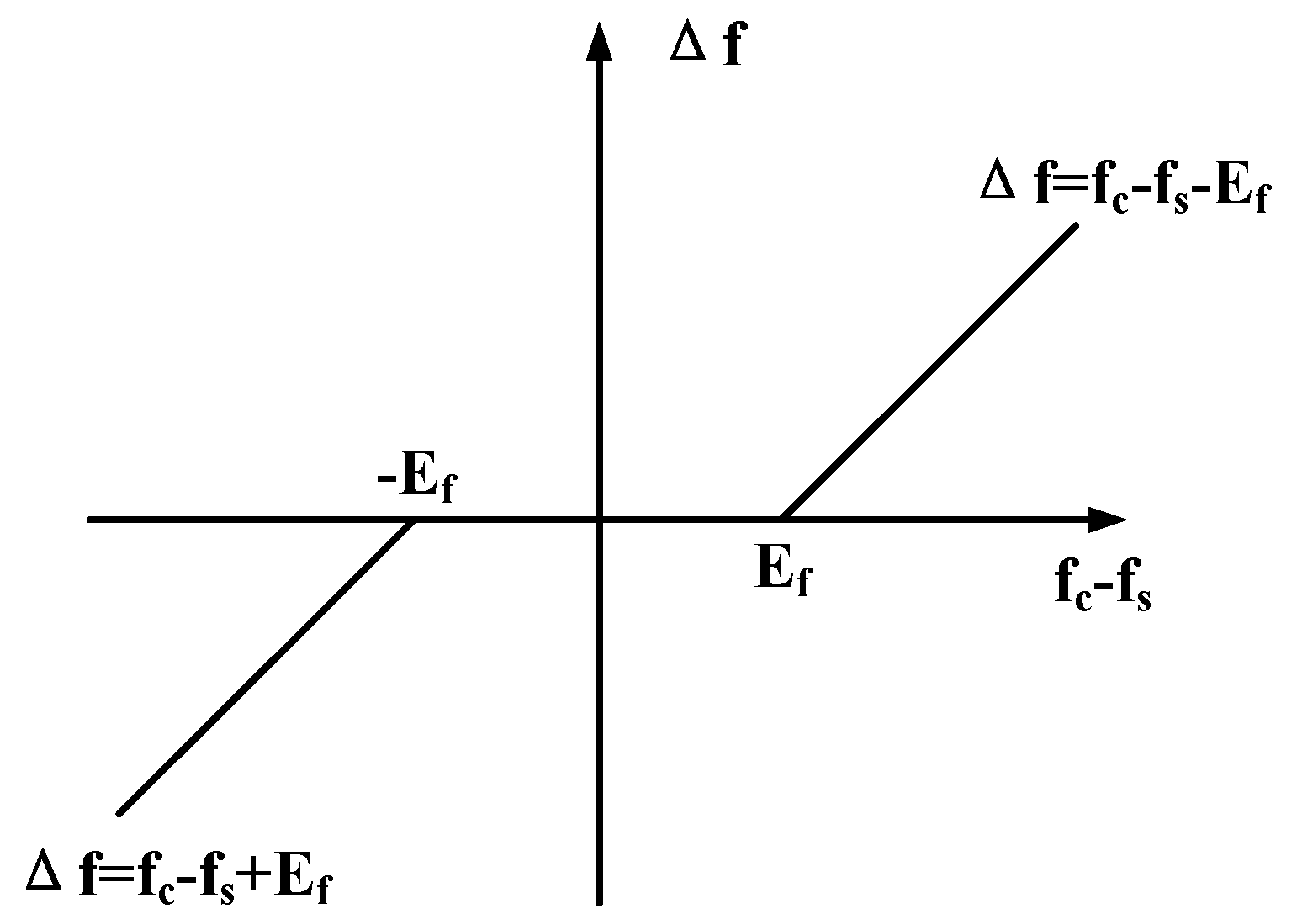
Figure 4.
The enhanced frequency dead zone proposed by a previous work.

Figure 5.
The improved frequency dead zone proposed in this paper.
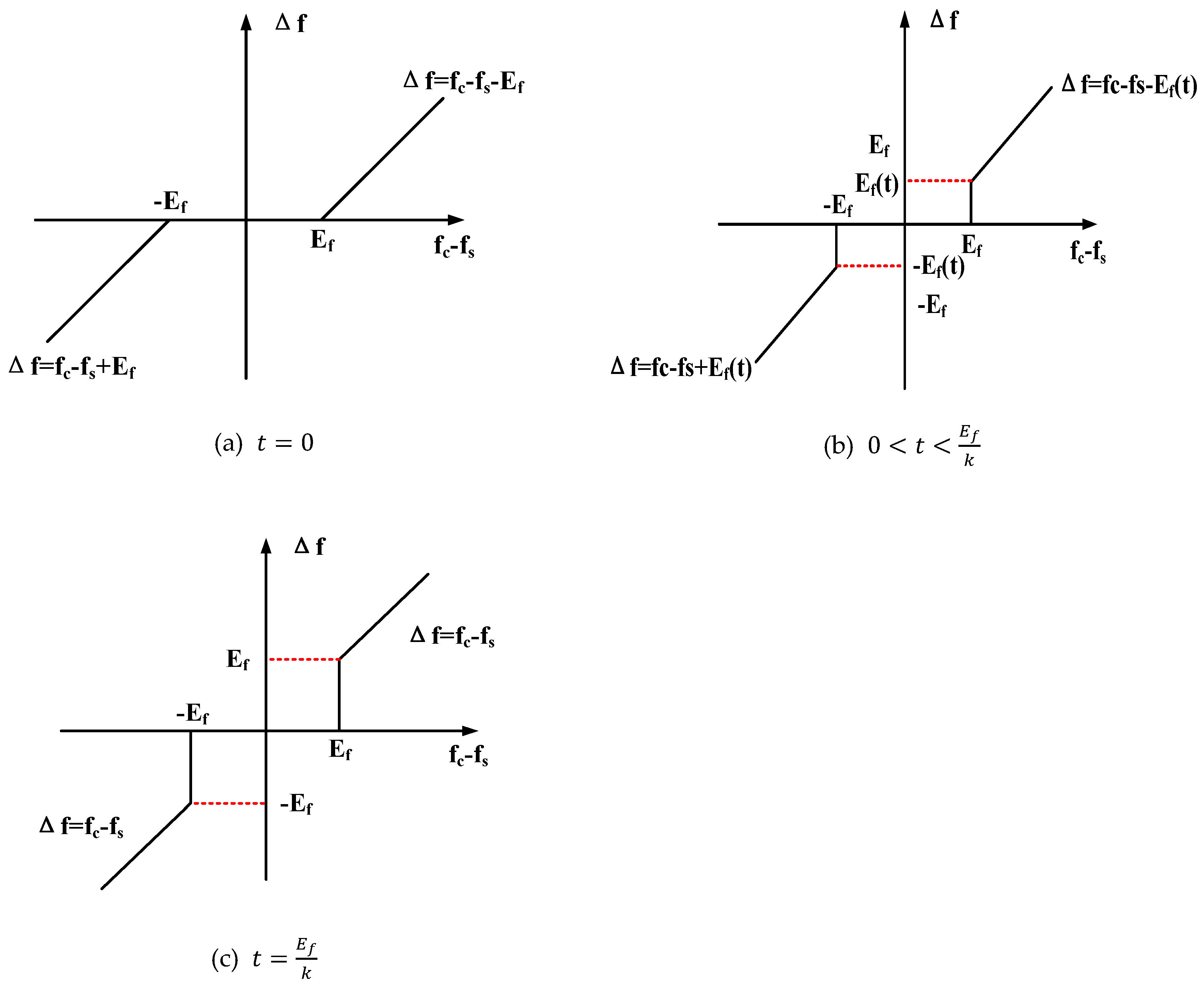
Figure 6.
The regulator model with common, enhanced, and improved dead zones and feed-forward control; is the regulation ratio; is the given power; is the real power; is the power dead zone; is the integral gain for feed-forward control.
Figure 6.
The regulator model with common, enhanced, and improved dead zones and feed-forward control; is the regulation ratio; is the given power; is the real power; is the power dead zone; is the integral gain for feed-forward control.
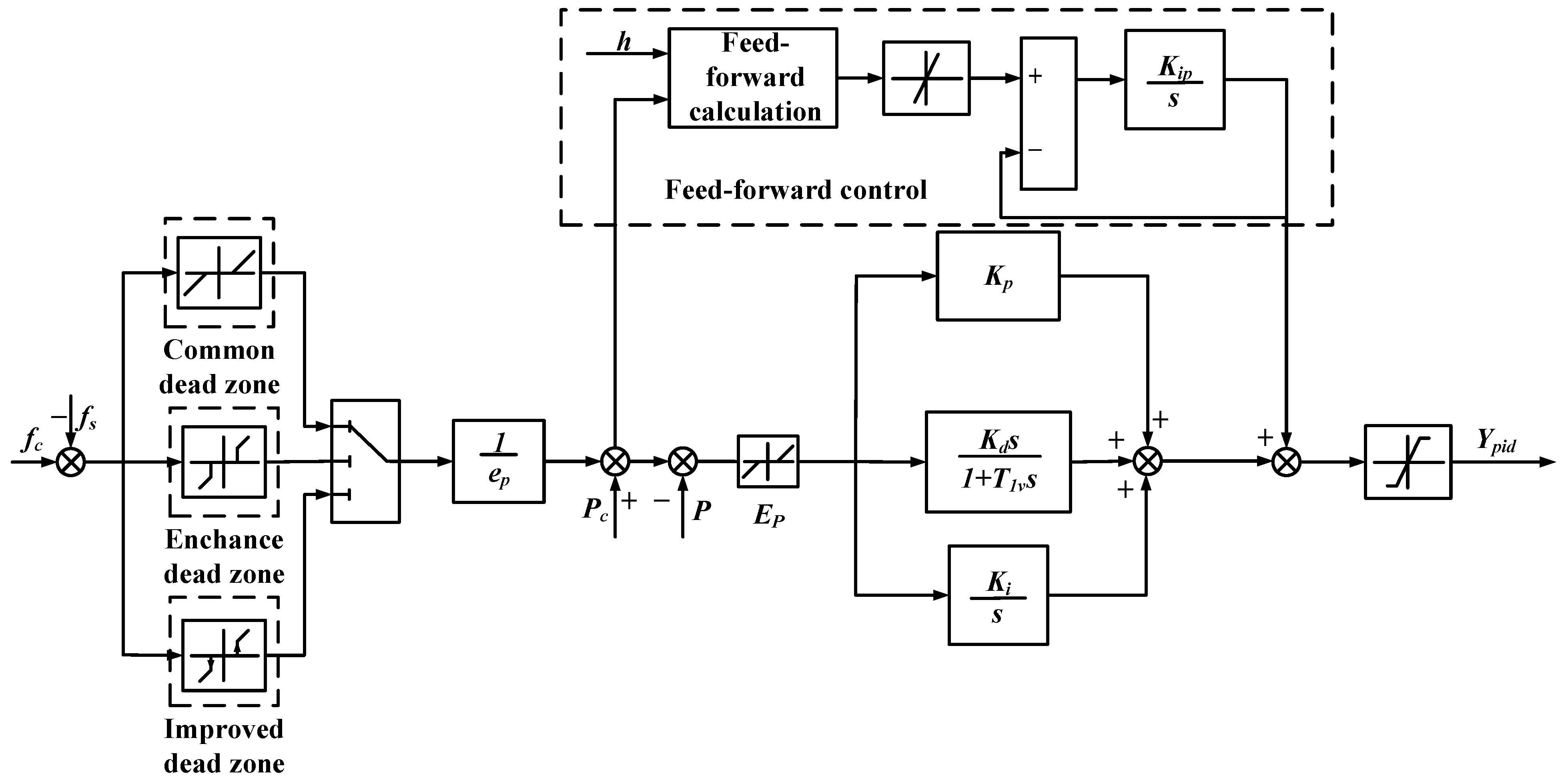
Figure 7.
Integrated control mode of power and frequency.
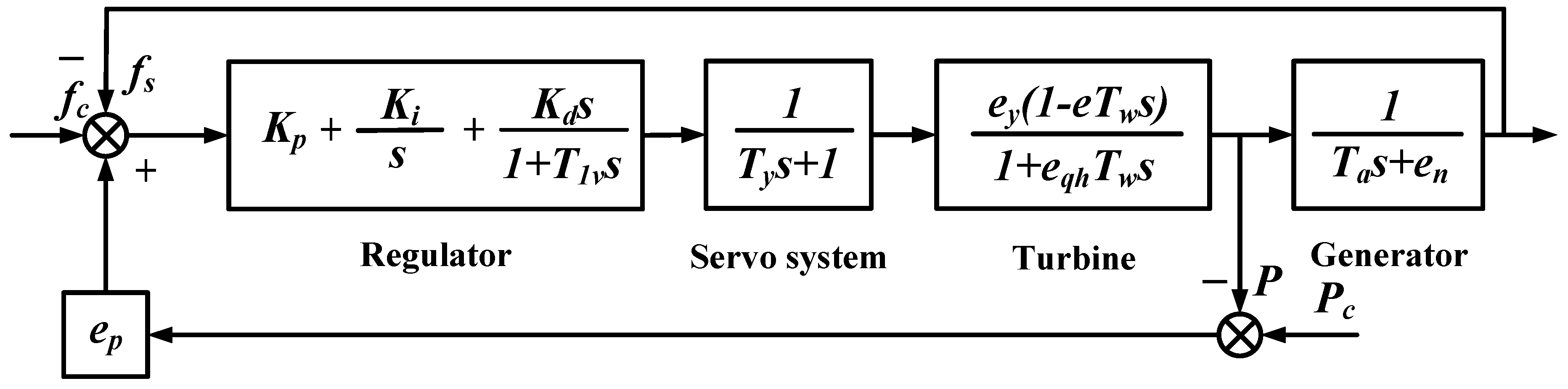
Figure 8.
Selective control mode of frequency and power.
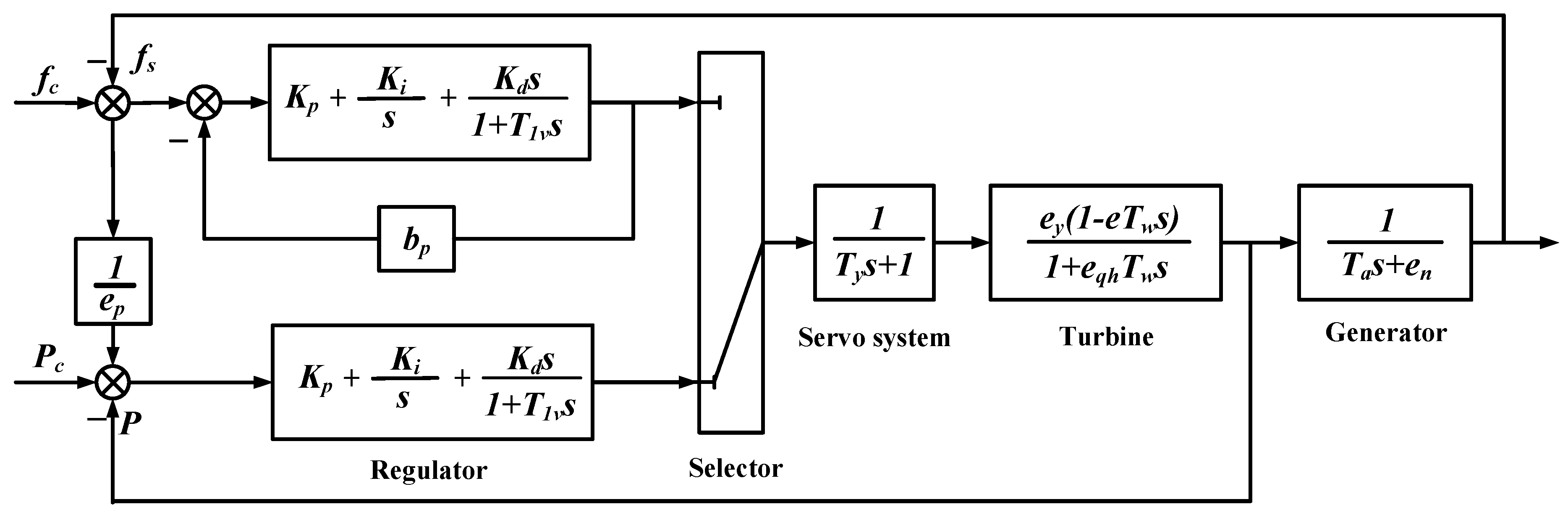
Figure 9.
The cam relationship of this paper.

Figure 10.
The relationship among unit discharge, guide vane opening, and unit rotation speed when the blade angle is 14 degrees.
Figure 10.
The relationship among unit discharge, guide vane opening, and unit rotation speed when the blade angle is 14 degrees.
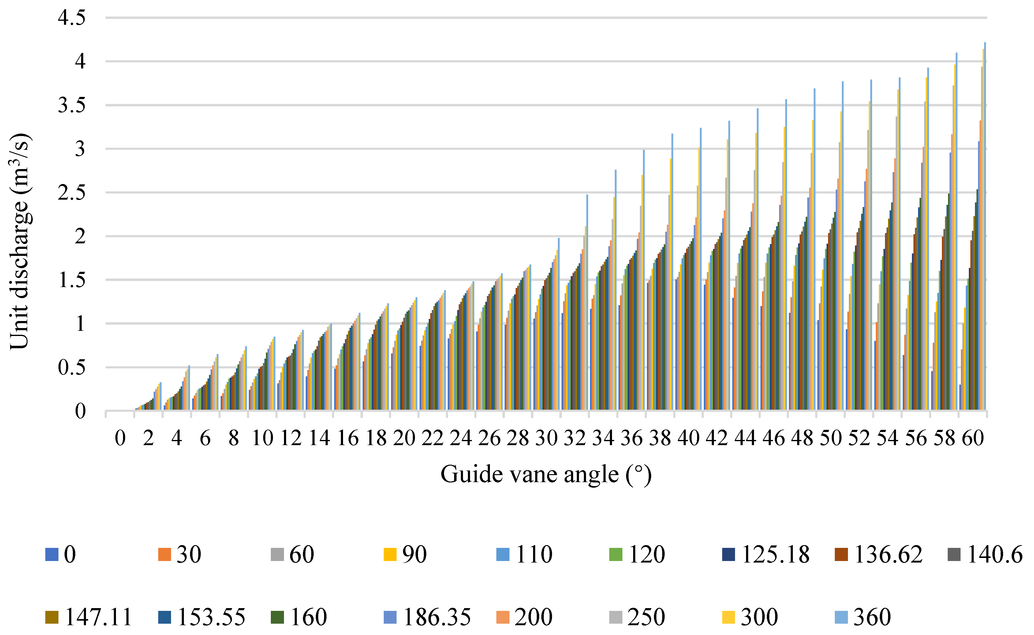
Figure 11.
The relationship among the unit hydraulic torque, the guide vane opening, and the unit rotation speed when the blade angle is 14 degrees.
Figure 11.
The relationship among the unit hydraulic torque, the guide vane opening, and the unit rotation speed when the blade angle is 14 degrees.
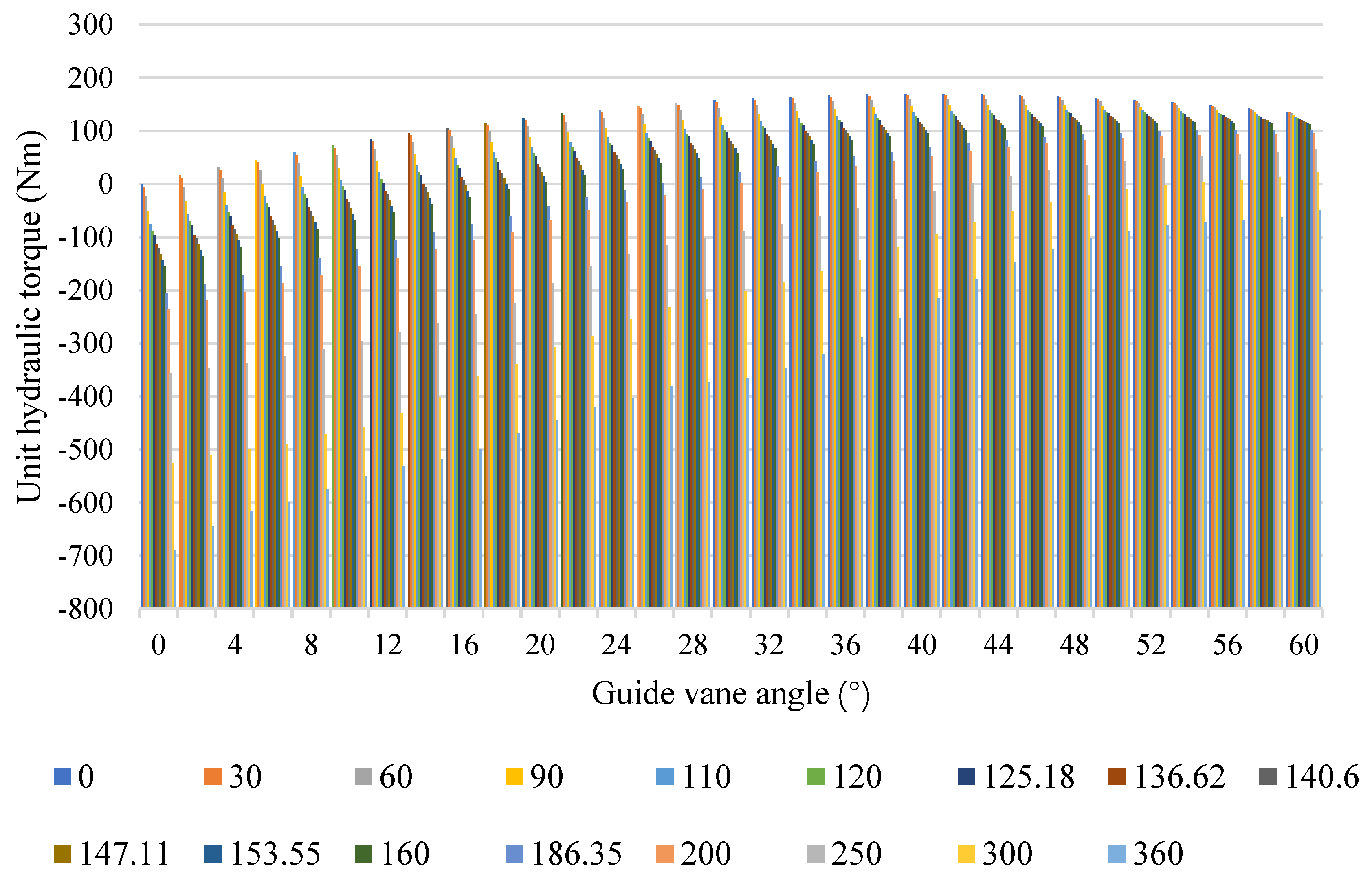
Figure 12.
Comparison of active power change between hydropower plants (HPP) and the simulation model when the step signal is ±0.065 Hz.
Figure 12.
Comparison of active power change between hydropower plants (HPP) and the simulation model when the step signal is ±0.065 Hz.

Figure 13.
Comparison of active power change between HPP and the simulation model when the step signal is ±0.055 Hz.
Figure 13.
Comparison of active power change between HPP and the simulation model when the step signal is ±0.055 Hz.
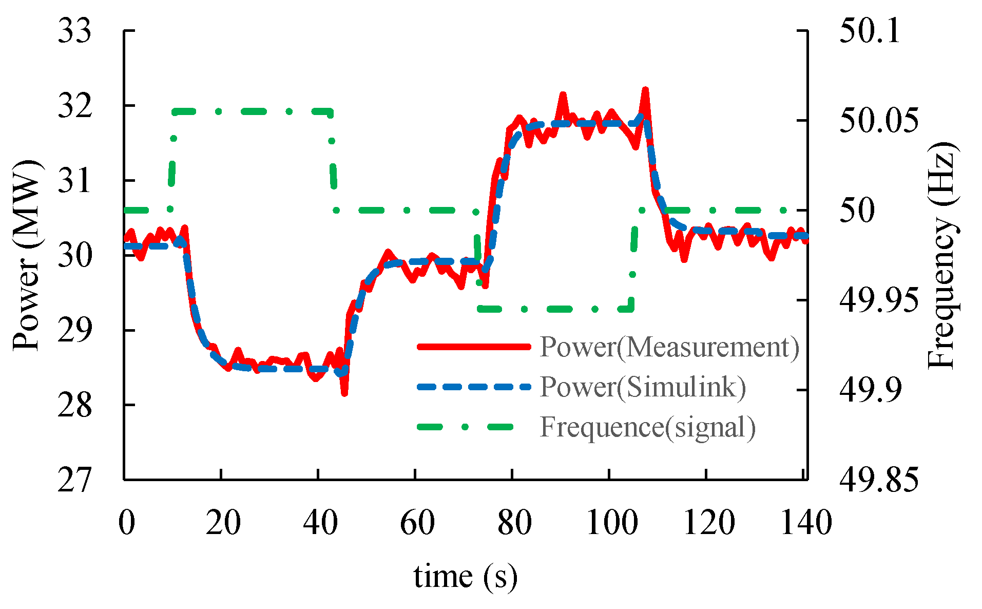
Figure 14.
The guide vane opening curve of primary frequency control (PFC) with common, enhanced, and improved frequency dead zones.
Figure 14.
The guide vane opening curve of primary frequency control (PFC) with common, enhanced, and improved frequency dead zones.

Figure 15.
The blade angle curve of PFC with common, enhanced, and improved frequency dead zones.

Figure 16.
The active power curve of PFC with common, enhanced, and improved frequency dead zones.

Figure 17.
The guide vane opening curve of PFC with common frequency dead zone, enhanced frequency dead zone with feed-forward control, and improved frequency dead zone with feed-forward control.
Figure 17.
The guide vane opening curve of PFC with common frequency dead zone, enhanced frequency dead zone with feed-forward control, and improved frequency dead zone with feed-forward control.
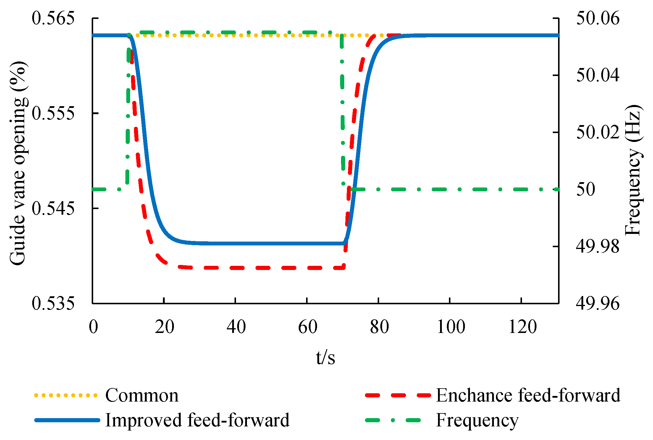
Figure 18.
The blade angle curve of PFC with common frequency dead zone, enhanced frequency dead zone with feed-forward control, and improved frequency dead zone with feed-forward control.
Figure 18.
The blade angle curve of PFC with common frequency dead zone, enhanced frequency dead zone with feed-forward control, and improved frequency dead zone with feed-forward control.
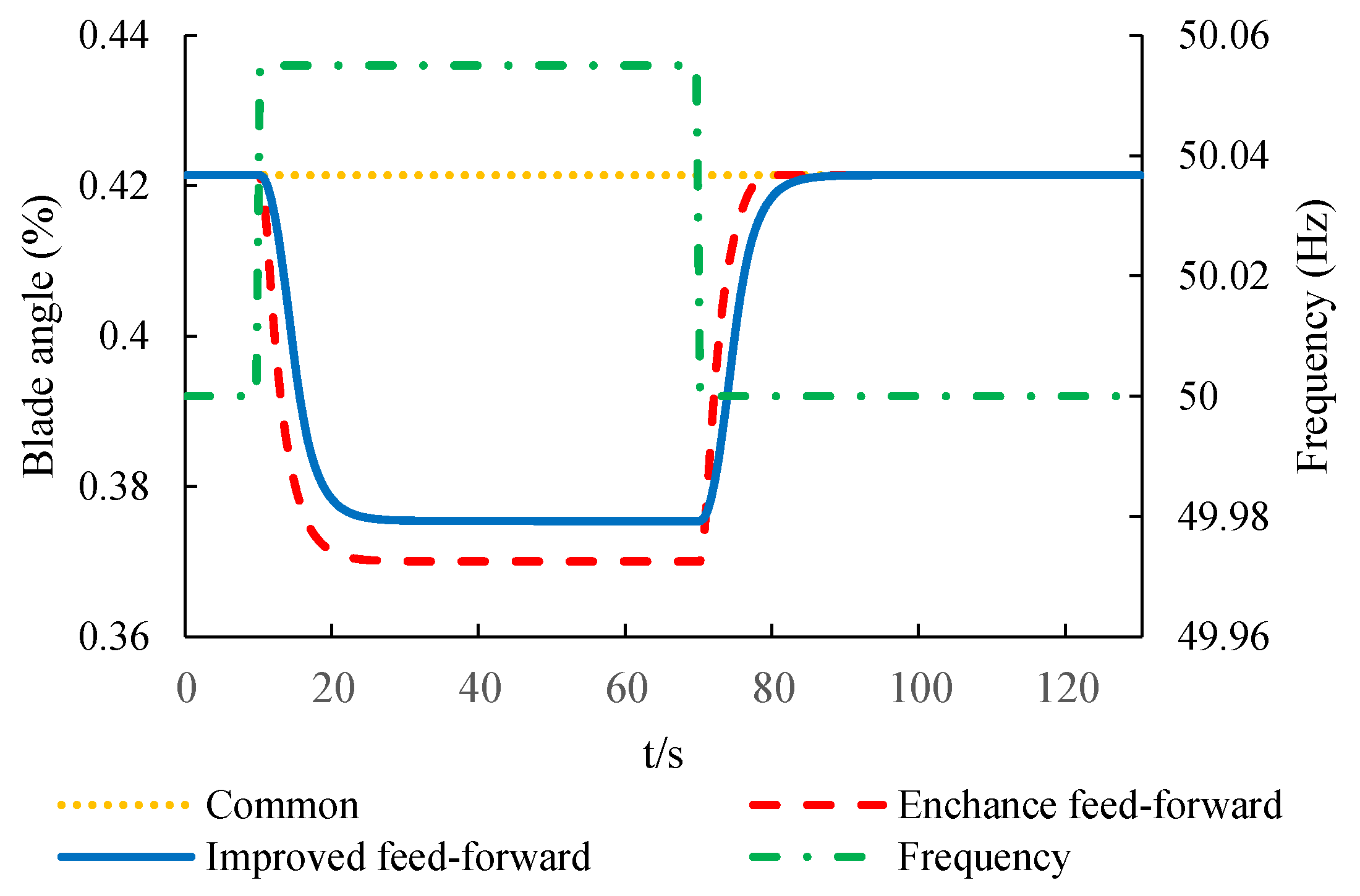
Figure 19.
The active power curve of PFC with common frequency dead zone, enhanced frequency dead zone with feed-forward control, and improved frequency dead zone with feed-forward control.
Figure 19.
The active power curve of PFC with common frequency dead zone, enhanced frequency dead zone with feed-forward control, and improved frequency dead zone with feed-forward control.
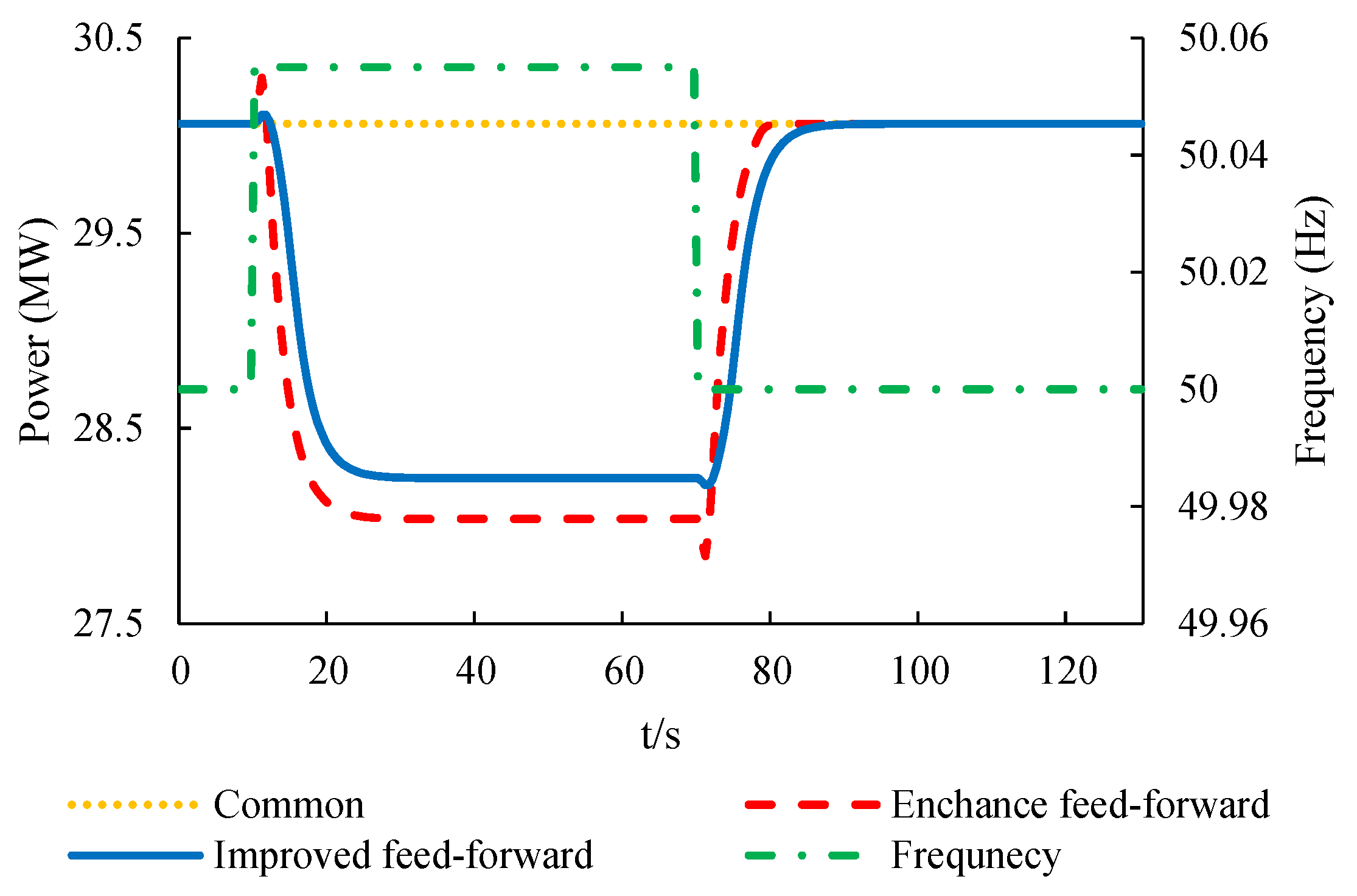
Figure 20.
PFC Indicators for Different Frequency Dead Zones. *IQE = integral quantity of electricity.
Figure 20.
PFC Indicators for Different Frequency Dead Zones. *IQE = integral quantity of electricity.
© 2019 by the authors. Licensee MDPI, Basel, Switzerland. This article is an open access article distributed under the terms and conditions of the Creative Commons Attribution (CC BY) license (http://creativecommons.org/licenses/by/4.0/).
Share and Cite
MDPI and ACS Style
An, H.; Yang, J.; Yang, W.; Cheng, Y.; Peng, Y. An Improved Frequency Dead Zone with Feed-Forward Control for Hydropower Units: Performance Evaluation of Primary Frequency Control. Energies 2019, 12, 1497. https://doi.org/10.3390/en12081497
AMA Style
An H, Yang J, Yang W, Cheng Y, Peng Y. An Improved Frequency Dead Zone with Feed-Forward Control for Hydropower Units: Performance Evaluation of Primary Frequency Control. Energies. 2019; 12(8):1497. https://doi.org/10.3390/en12081497
Chicago/Turabian StyleAn, Hao, Jiandong Yang, Weijia Yang, Yuanchu Cheng, and Yumin Peng. 2019. "An Improved Frequency Dead Zone with Feed-Forward Control for Hydropower Units: Performance Evaluation of Primary Frequency Control" Energies 12, no. 8: 1497. https://doi.org/10.3390/en12081497
Note that from the first issue of 2016, this journal uses article numbers instead of page numbers. See further details here.