Probabilistic Estimation of the Energy Consumption and Performance of the Lighting Systems of Road Tunnels for Investment Decision Making

Abstract

This paper presents a probabilistic model for supporting the process of decision making about the value of new lighting systems in existing road tunnels when some data and parameters are affected by uncertainty. The proposed model, which we have called Probabilistic Energy Screening of Tunnel (PrEST), accounts for both the technical performance and the economic objectives of the new lighting systems. The technical performance is described on an adequate (x, y) plane that was defined by two indices. The first index measured the consumption of electricity per kilometre of tunnel lengths; the second index measured the performance of the lighting systems per unit of illuminated area. The economic results were measured by the net present value of the savings and by the payback period. Both the terms account for initial capital investments, energy and maintenance costs. PrEST was applied to two real road tunnels in service in Italy showing that the statistics of the results can support a final decision in function of the business strategy.

1. Introduction

Adequate levels of visibility on roads allow pedestrians to walk minimizing the risk of accidents; further, in the town, they can also enjoy the space around perceiving a sense of security against aggressions or thefts [1]. The lighting systems of roads and tunnels are essential for the security of the citizens and for the safety of the drivers. Good luminosity on roads and in tunnels is strictly linked to the safety of the vehicle driving. The driver must be able to detect the presence of obstacles, to perceive any changes in driving conditions without developing a sense of uncertainty or, even worse, fear.

With reference to the safety of vehicle driving, National and International Standards, such as those of the Commission Internationale de l’Eclairage (CIE), state the requested levels of minimum illuminance within accepted boundaries for limiting other aspects like glare or the lack of vertical uniformity. In particular, the lighting systems of a tunnel (LSTs) must be designed following the minimum luminance profile, as reported by the European Standard [2]. The standard gives the required values of the luminance along the longitudinal axis of the tunnel versus the travel time along the tunnel at the reference speed (the reference speed is equal to the speed limit in the tunnel; the value is provided by the operator of the road where the tunnel is in service), as Figure 1 shows.

The performance of the lighting system for a LST in terms of quantity and quality of luminosity is only one of the principal aspects to account for in the design stage. The further aspect refers to the energy consumption.

The LSTs represent the most electricity-consuming loads for the companies that manage the primary roads. Surveys show that lighting consumes 30% of the energy consumed by the mechanical and electrical systems in highway tunnels and that the tunnel lighting costs are a loss for tunnel management departments [3,4].

Technological innovations in lamps with the introduction on the market of solid state lamps using Light Emitting Diodes (LEDs) has certainly reduced the problem of energy consumption, but it did not erase it at all. LEDs are surely characterized by an increased efficiency value measured in lumen/Watt (lm/W), but the particular applications of these lamps in the tunnels still requires the installation of solid state lamps with a high power value, even if lower than those of gas discharge lamps with the same lumens.

The companies that manage a large set of tunnels have the problem of sorting the LTSs for planning investments over a defined time horizon. The optimal sorting must consider both the technical requirements and the need for the reduction of the energy consumption.

In the specialized literature, the aspect of energy consumption of LSTs has been faced from different points of view [5,6,7,8,9]. In [5], the authors dealt with the energy requirements of the lighting systems in emergency conditions when an accident occurs. They show a case study in which the energy consumption for back-up and safety of the emergency lighting are covered by means of photovoltaic panels, generating a cash flow able to pay back the extra investment in photovoltaics. The contribution [6] proposes the estimation of the energy consumptions of the LSTs in the design stage taking properly into account the advantages of the power consumption savings obtainable by internal luminance regulation.

Paper [7] proposes improving the global performance of the lighting systems in a tunnel, by using new road paving materials characterized by a higher reflection coefficient than other ordinary asphalts.

In [8,9], the Energy Screening of Tunnel (EST) model was introduced to handle both the aspects of reducing the energy consumption and improving the lighting performance, in an integrated way. EST allows representing every LST in a Cartesian plane {electricity consumption, performance} introducing appropriate indices. In [9] the results of the EST model were also verified by means of experimental measurements on the road. The EST model was not a tool for designing new LST. EST, instead, was a valuable mean for sorting the decision of the investments to make on several existing LSTs taking into account both the average lighting performance and the average energy consumption.

In this paper, starting from the initial versions of EST presented in [8,9], we first improved the model by including an economic module. This economic module allows comparing the investments required for improving the energy efficiency and the lighting performance of any LST. By using the economic module one can have an idea of the cost associated with different technical solutions capable of improving the performance of the LST in terms of consumption and lighting efficiency. Then, we dealt with the further problem that really can condition the decision of the investments: the uncertainty that affects some of the data of the problem. To this aim, we transferred the model EST on a probabilistic basis and propose Probabilistic Energy Screening of Tunnel (PrEST). In particular, we first analyse the most important EST input data and parameters that require the introduction of random variables. Then, the probabilistic technique of analysis is described in details.

The paper is structured as follows: EST is recalled in Section 2 showing the advancements in respect to the preceding papers [8,9]; the probabilistic modelling PrEST is presented in Section 3; some numerical results are shown in Section 4 with reference to some LSTs actually in service in Italy.

2. Recall and Improvements of the Model EST

The EST model presented in [8,9] was improved by integrating a section for economic evaluations; the new version of EST consists of two modules, namely the technical module, TM, and the economic module, EM (Figure 2).

TM, based on the model developed in [8,9], allows representing any LST on the same Cartesian plane {electricity consumption, performance}. The objective of the TM was the derivation of two indices, one linked to the average lighting performance of the LST, the other linked to the average power consumption. The choice of these indices was motivated by the need to represent on the same Cartesian plane {electricity consumption, performance} every LST, using the actual service conditions and in the new service conditions due to possible interventions. Such a representation on the same Cartesian plane allowed comparing several LSTs with each other, and for the same LST, different possible interventions for making decisions on a long time horizon, when several LSTs are managed by the same company. TM is not a tool for designing a LST.

EST was conceived as a tool for supporting the decisions of the manager of several LSTs about the investments for upgrading them both for the illumination performance and for the energy consumption, providing a screening of their operating conditions (current conditions and estimated future conditions linked to possible alternative interventions) without performing detailed in field measurements. This is the great advantage of using EST according to the methods usually adopted for having information and data on the current operating conditions of several LSTs. Usually, the managing company must measure the luminance in the field. This is a very expensive activity in time, in human resources, and indirect costs linked to the need for limiting, deviating or stopping the traffic. EM, added in this paper to EST, allows comparing the investments faced for improving the energy efficiency and the lighting performance of any LST.

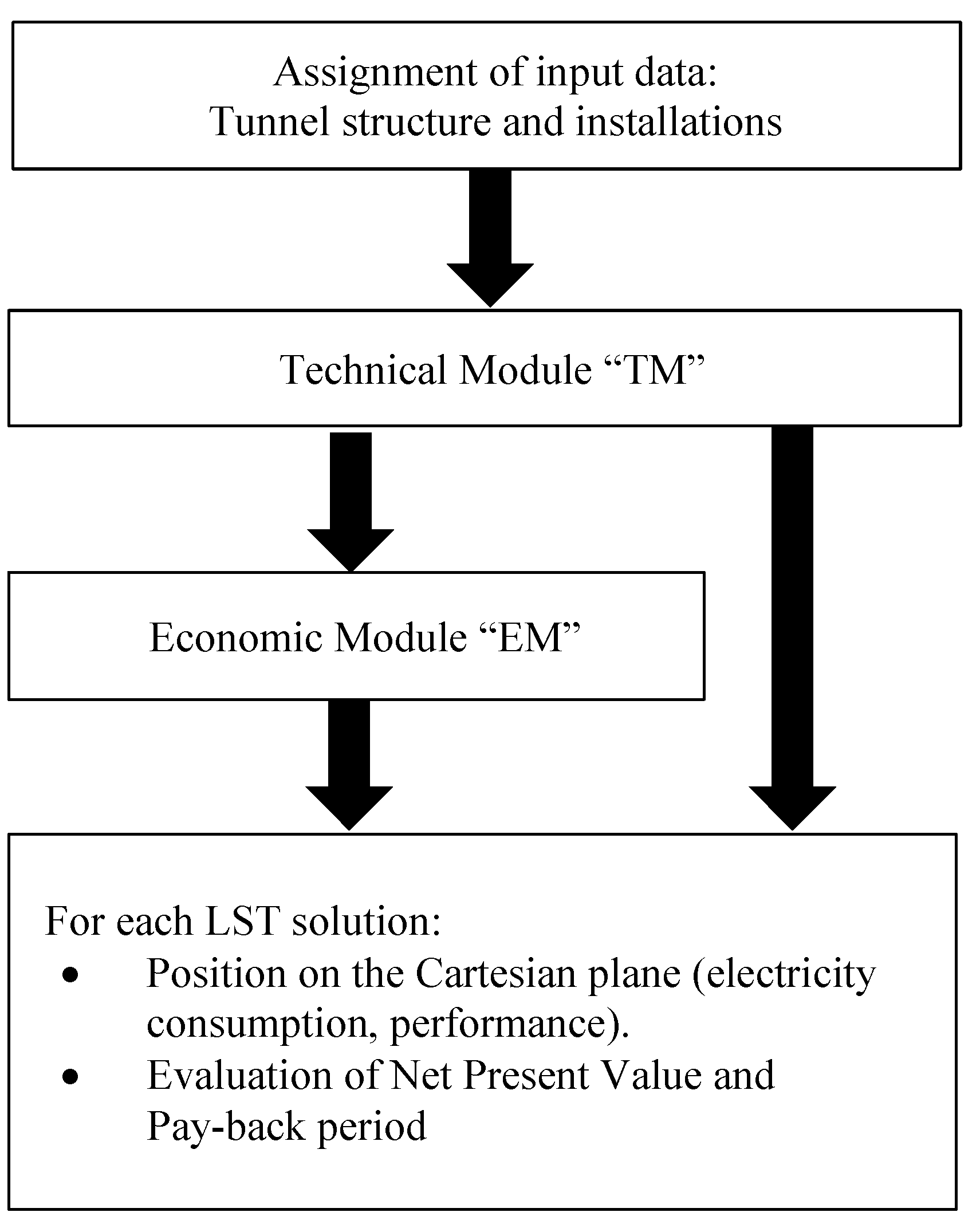
2.1. The Technical Module TM

The key idea at the basis of the TM of EST was to represent any LST on the same Cartesian plane {electricity consumption, performance} by means of proper variation indices with the respect to the LST of reference, namely the LST* [10].

The choice of the LST* was effected on the basis of the incentives given in Italy to promote the energy efficiency investments. The national authority for the regulation on the energy, Autorità di Regolazione per Energia, Reti e Ambiente (ARERA, formerly AEEG) stated with the resolution [10] in which cases financial incentives were recognized for installing new LSTs. Note that in other countries, the LST* can be different in function of the local regulations. For example, in [11] different strategies for supporting the investments on energy efficiency in the different USA states are listed and commented.For the primary roads, three types of structure of LST were defined as baseline cases. They are the LSTs whose performance, in terms of energy consumptions and lighting, must be overcome for obtaining the incentives. Each baseline was proposed by ARERA with characteristics adequate for guarantying the respect of the European Standard [2]. The main characteristics of the baseline cases proposed by ARERA in [10] are listed below. The data common to every LST* are:

-

100 W sodium high pressure (SHP) lamps, with 14 W of auxiliary circuits, reduced power during the night to 59 W with invariant power of auxiliary circuits;

-

efficiency equal to 61 lm/W;

-

the lamps have a color rendering index not greater than 60 so that the lighting category of the road is not reduced;

-

13 h of operation during the morning, 11 h of operation during the night, 365 days of annual operation;

-

height of whitewashed walls equal to 3.0 m;

-

LSTs which have the lines of luminaires equipped with lamps placed sideways are assimilated to the ones with luminaires equipped with lamps placed in line above the roadway:

-

for the short tunnels, e.g., those according to [2] of length up to 125 m, the lighting level is assumed equal to 100% of that provided for the long galleries.

The characteristics different for each of the baseline cases reported in [10] are:

-

single central line of luminaries with 10 m of spacing, 100 luminaires/Km;

-

double central line of luminaries with 9 m of spacing, 222 luminaires/Km;

-

triple central line of luminaries with 9 m of spacing, 333 luminaires/Km.

Starting from the baseline cases proposed by ARERA in [10], we extended the baseline cases for covering most of the actual roads in operation, that is dual or single carriageway, single-way or double-way road with different speed limit values, and considering the three possible configurations of the lines of luminaires (single, double or central line). For all the baseline cases, comprising those proposed by ARERA in [10], we firstly developed the models for using the freeware program Dialux [12], not available in the Dialux library. By means of Dialux, the luminance profile of every baseline was verified in accordance with the standard [2]. In so doing, we realized a library of baseline cases, LST*, for comparing any LST in the study with them.

For every LST* of the baseline library, we computed two indices of reference: LP_i* and EC_i*. LP_i* is the average illuminance for each square meter of the LST_i; EC_i*, is the annual energy consumption per kilometer of the LST_i*.

With reference to Figure 2, the TM starts with the assignment of the data of the tunnel, of the road, and of the LST. The main data to assign are: length, width and height for the tunnel; dual carriageways or single carriageways, and speed limit for the road; structure (single central line, double central line, triple central line) and characteristics of the lamps (power, efficiency, auxiliary systems) for the LST.

For every LST_i, we computed the energy consumption index, ECi, and the illuminance index, LPi. Finally, considering the baseline LST_i* corresponding to every LST in study, it was possible to compute the following variation indices:

∆EC_i = EC_i − EC_i*

(1)

∆LPI_i = LP_i − LP_i*

(2)

If ∆EC_i is greater than zero, the consumption must be reduced; otherwise, the consumption is acceptable. In a similar way, if ∆LP_i is less than zero, the lighting performance has to be improved otherwise it is acceptable.

The important result of the TM, which was an intermediate result of EST, is the representation of every LST on the Cartesian plane shown in Figure 3 where three LSTs were represented [9]. It is evident that no LST falls in the second quadrant where both the energy consumption and the lighting performance are acceptable.

The LST corresponding to the green triangle requires a reduction of the energy consumption, the LSTs corresponding to the red square and to the blue rhombus primarily need improved lighting performance.

Once obtained the characterization of every LST on the Cartesian plane of Figure 3, the TM allows evaluating the new values of (∆EC_i)_k and (∆LP_i)_k for any kth possible intervention aimed to reduce the energy consumption and improve the lighting performance. Using Equations (1) and (2) in which the reference values LP_i* and EC_i* are unchanged, it is possible, for every solution k to implement in every LSTi, the computation of the new value of the indices (∆EC_i)_k and (∆LP_i)_k. By so doing, we can verify if any of the possible intervention can drive each LSTi in the second quadrant.

Figure 4 is an example of the results obtainable for one of the three LSTs represented in Figure 3. In particular, Figure 4 shows the effects of two different interventions that were considered to improve the LST represented in Figure 3 with the green triangle. The considered alternatives were:

-

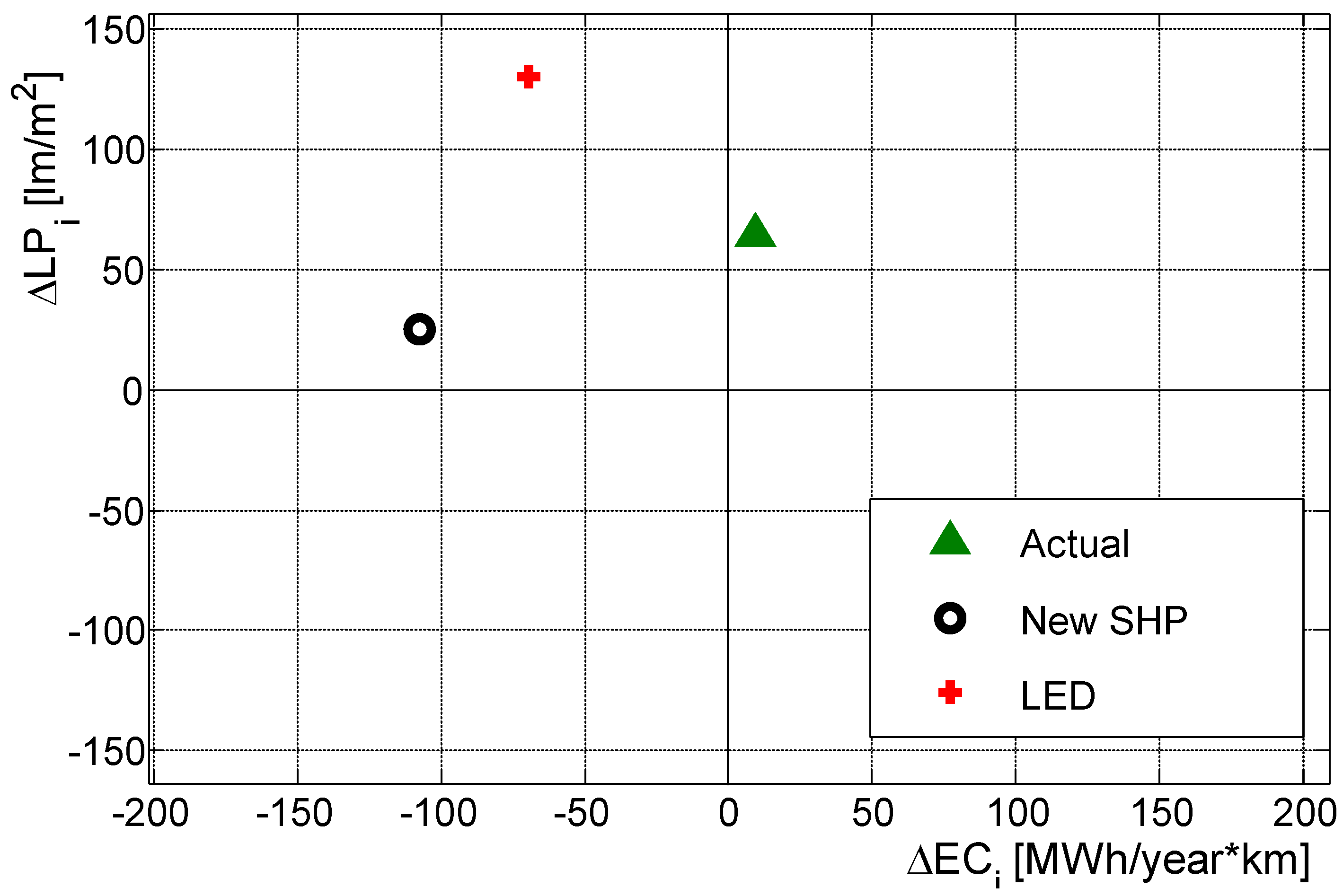
New SHP: substituting sodium high-pressure discharge (SHP) with higher efficiency for the existing SHP;

-

LED: substituting LED luminaires (SHP) for the existing SHP.

It is evident from Figure 4 that all the interventions improve the LST operation, in fact, the points representative of the modified LSTs belong to the second quadrant. To support the final decision on the investment to face among those solutions, which improved the performance of each LSTi, EST runs the economic module EM, described in the following section.

2.2. The Economic Module EM

The EM starts with the assignment of the data for the possible solutions which resulted in the TM adequate for improving both the indices, (∆EC_i)_k and (∆LP_i)_k. For each LST_i some possible solutions can be installing flux regulators on the existing lamps and luminaires, substituting lamps and luminaires with higher luminous efficacy for the existing ones, or installing new lamps and luminaires with flux regulators or dimmers. Note that in the following, to avoid verbose notation the subscript i referred to index tunnel, will not be used.

For every kth solution, the main data are: power, luminous efficacy, number, useful life, total cost of the lamps, the luminaires and the auxiliaries, cost of the maintenance, tariff of the energy, and so on. All these data permit the computation of the cost of the existing LST, named annual cost of the old solution ${\left({\mathrm{KA}}_{\mathrm{n}}\right)}_{\mathrm{OS}}$ to face in the year n, and of the improved (LST_i)_k, named annual cost of the new kth solution ${\left({\mathrm{KA}}_{\mathrm{n}}\right)}_{\mathrm{k}}$ to face in the year n.

For the computation of the annual costs of the old solution and of any new solution, the economic model of the CIE [13] defines the hourly cost of an LST taking into account all the components of cost arising during the annual operation from the costs for installation to those for the maintenance. This model of the cost is very valuable when the cost and saving estimation is performed on a one-year basis.

When the financial analysis is extended in a time period longer than one year, the economic model of the annual cost of the old solution and of any new solution is more effective if the costs of the investments are separated from the other costs. This choice allows for estimating the cash flow taking into account the time value of the money. With this choice, the annual cost ${\left({\mathrm{KA}}_{\mathrm{n}}\right)}_{\mathrm{OS}}$ and ${\left({\mathrm{KA}}_{\mathrm{n}}\right)}_{\mathrm{k}}$ faced in the year i are:

$${\left({\mathrm{KA}}_{\mathrm{n}}\right)}_{\mathrm{os}}={\left({\mathrm{KAI}}_{\mathrm{n}}\right)}_{\mathrm{os}}+{\left({\mathrm{KAO}}_{\mathrm{n}}\right)}_{\mathrm{os}}$$

(3)

$${\left({\mathrm{KA}}_{\mathrm{n}}\right)}_{\mathrm{k}}={\left({\mathrm{KAI}}_{\mathrm{n}}\right)}_{\mathrm{k}}+{\left({\mathrm{KAO}}_{\mathrm{n}}\right)}_{\mathrm{k}}$$

(4)

where (KAI_n)_os and (KAI_n)_k are the costs for acquiring and installing the lamps ${\left({\mathrm{CLamp}}_{\mathrm{n}}\right)}_{\mathrm{os}}$ and the luminaires ${\left({\mathrm{CLum}}_{\mathrm{n}}\right)}_{\mathrm{os}}$ of the old solution, and of any new k solution ${\left({\mathrm{CLamp}}_{\mathrm{n}}\right)}_{\mathrm{k}}$ and ${\left({\mathrm{CLum}}_{\mathrm{n}}\right)}_{\mathrm{k}}$, respectively; (KAO_n)_os and (KAO_n)_k are the other costs to face in each year for the old solution and for any new k solution.

The costs (KAO_n)_os and (KAO_n)_k are derived from the hourly costs ${\left({\mathrm{KAO}}_{\mathrm{nh}}\right)}_{\mathrm{os}}$ and ${\left({\mathrm{KAO}}_{\mathrm{nh}}\right)}_{\mathrm{k}}$ as:

$${\left({\mathrm{KAO}}_{\mathrm{n}}\right)}_{\mathrm{os}}={\left({\mathrm{KAO}}_{\mathrm{nh}}\right)}_{\mathrm{os}}\ast \mathrm{H}$$

(5)

$${\left({\mathrm{KAO}}_{\mathrm{n}}\right)}_{\mathrm{k}}={\left({\mathrm{KAO}}_{\mathrm{nh}}\right)}_{\mathrm{k}}\ast \mathrm{H}$$

(6)

where H is the number of operation hours during each year n.

The expression of the hourly cost in the year n, (K_nh)_j for any j solution is given by:

$${\left({\mathrm{K}}_{\mathrm{ih}}\right)}_{\mathrm{j}}={\left({\mathrm{CMat}}_{\mathrm{ih}}\right)}_{\mathrm{j}}+{\left({\mathrm{CEn}}_{\mathrm{ih}}\right)}_{\mathrm{j}}+{\left({\mathrm{CMaint}}_{\mathrm{ih}}\right)}_{\mathrm{j}}+{\left({\mathrm{CF}}_{\mathrm{ih}}\right)}_{\mathrm{j}}$$

(7)

$$\mathrm{with}\mathrm{j}=\{\begin{array}{c}\mathrm{os} \mathrm{for} \mathrm{the} \mathrm{old} \mathrm{solution}\\ \mathrm{k} \mathrm{for} \mathrm{any} \mathrm{new} \mathrm{solution}\end{array}$$

In Equation (7) (CMat_nh)_j is the hourly cost in the year n of all the materials with the exclusion of the lamps and luminaires, ${\left({\mathrm{CEn}}_{\mathrm{nh}}\right)}_{\mathrm{j}}$ is the hourly cost in the year i of the electric energy consumptions, ${\left({\mathrm{CMaint}}_{\mathrm{nh}}\right)}_{\mathrm{j}}$ is the hourly cost in the year n of the maintenance, ${\left({\mathrm{CF}}_{\mathrm{nh}}\right)}_{\mathrm{j}}$ is the hourly cost of further possible interventions. The Appendix A presents the expressions of the terms in the Equation (7).

Considering the Equations (3) and (4) with the position (5), the general expressions of the annual cost of the year n of the old solution and of any new k solution are:

$${\left({\mathrm{KA}}_{\mathrm{n}}\right)}_{\mathrm{os}}={\left({\mathrm{KAI}}_{\mathrm{n}}\right)}_{\mathrm{os}}+{\left({\mathrm{KAO}}_{\mathrm{nh}}\right)}_{\mathrm{os}}\ast \mathrm{H};$$

(8)

$${\left({\mathrm{KA}}_{\mathrm{n}}\right)}_{\mathrm{k}}={\left({\mathrm{KAI}}_{\mathrm{n}}\right)}_{\mathrm{k}}+{\left({\mathrm{KAO}}_{\mathrm{nh}}\right)}_{\mathrm{k}}\ast \mathrm{H}.$$

(9)

Starting from the knowledge of the annual cost of the old solution, ${\left({\mathrm{KA}}_{\mathrm{n}}\right)}_{\mathrm{OS}}$, and of each kth new solution, ${\left({\mathrm{KA}}_{\mathrm{n}}\right)}_{\mathrm{k}}$, EM allows performing the financial analysis. In the actual version, EM evaluates two main financial quantities for the alternative k. They are the net present value of the total savings, NPVS_k and the discounted payback period, PB_k.

The NPVS_k is the current worth of the future saving of money or stream of cash flow, given a specified rate of return $\mathsf{\alpha }$. Considering a period of N years in which we perform the financial evaluation. For every new solution k, the NPVS_k is given by:

$${\mathrm{NPVS}}_{\mathrm{k}}={\displaystyle \sum }_{\mathrm{n}=1}^{\mathrm{N}}\frac{\left[{\mathrm{DKA}}_{\mathrm{n}}+\left({\mathrm{DCEn}}_{\mathrm{n}}\ast {\left(1+\mathsf{\beta }\right)}^{\mathrm{n}-1}\right)\right]}{{\left(1+\mathsf{\alpha }\right)}^{\mathrm{n}-1}}$$

(10)

where is variation rate of the energy cost, ${\mathrm{DCEn}}_{\mathrm{n}}$ is the variation of the cost of electric energy of each year n given by:

$${\mathrm{DCEn}}_{\mathrm{n}}={\left({\mathrm{CEn}}_{\mathrm{n}}\right)}_{\mathrm{os}}-{\left({\mathrm{CEn}}_{\mathrm{n}}\right)}_{\mathrm{k}}$$

(11)

with ${\left({\mathrm{CEn}}_{\mathrm{n}}\right)}_{\mathrm{os}}={\left({\mathrm{CEn}}_{\mathrm{nh}}\right)}_{\mathrm{os}}\ast \mathrm{H}$ and ${\left({\mathrm{CEn}}_{\mathrm{n}}\right)}_{\mathrm{k}}={\left({\mathrm{CEn}}_{\mathrm{nh}}\right)}_{\mathrm{k}}\ast \mathrm{H}$.

In (10), ${\mathrm{DKA}}_{\mathrm{n}}$ is the variation of the annual costs between the old solution and the new kth solution given by:

$${\mathrm{DKA}}_{\mathrm{n}}={\left({\mathrm{KA}}_{\mathrm{n}}^{\prime }\right)}_{\mathrm{os}}-{\left({\mathrm{KA}}_{\mathrm{n}}^{\prime }\right)}_{\mathrm{k}}$$

(12)

where ${\left({\mathrm{KA}}_{\mathrm{n}}^{\prime }\right)}_{\mathrm{os}}$ and ${\left({\mathrm{KA}}_{\mathrm{n}}^{\prime }\right)}_{\mathrm{k}}$are the annual cost, other than the annual energy cost, to be incurred in each year n for the old solution and for the new solution, respectively.

The values of ${\left({\mathrm{KA}}_{\mathrm{n}}^{\prime }\right)}_{\mathrm{os}}$ and ${\left({\mathrm{KA}}_{\mathrm{n}}^{\prime }\right)}_{\mathrm{k}}$ depends on the year n since in each year we must include the cost of all the replacements, if any. For the old solution, we considered the cost of only the replacements of the existing lamps when they end their life; for the new solution we considered to replace all the materials only at the first year; for the successive years, we assumed to replace only the lamps. For any solution j, this implies that:

$${\mathrm{LLamp}}_{\mathrm{j}}\le \mathrm{N};{\mathrm{LLamp}}_{\mathrm{j}}=\frac{{\mathrm{LLamp}}_{\mathrm{j}}^{\mathrm{h}}}{8760},$$

(13)

$${\mathrm{LLum}}_{\mathrm{j}}>\mathrm{N};{\mathrm{LLum}}_{\mathrm{j}}=\frac{{\mathrm{LLum}}_{\mathrm{j}}^{\mathrm{h}}}{8760},$$

(14)

$${\mathrm{LMat}}_{\mathrm{j}}>\mathrm{N};{\mathrm{LMat}}_{\mathrm{j}}=\frac{{\mathrm{Lmat}}_{\mathrm{j}}^{\mathrm{h}}}{8760},$$

(15)

where ${\mathrm{LLamp}}_{\mathrm{j}}$, ${\mathrm{LLum}}_{\mathrm{j}}$, ${\mathrm{LMat}}_{\mathrm{j}}$ are the nominal life in years of lamps, luminaires and materials of the jth solution, respectively, and ${\mathrm{LLamp}}_{\mathrm{j}}^{\mathrm{h}}$, ${\mathrm{LLum}}_{\mathrm{j}}^{\mathrm{h}},{\mathrm{Lmat}}_{\mathrm{j}}^{\mathrm{h}}$ are the corresponding lives expressed in hours.

Let’s consider the number of substitution to face in the period N for the old solution, NS_os, and for any new solution k, NS_k; they are given by:

$${\mathrm{NS}}_{\mathrm{os}}=\lceil \frac{\mathrm{N}}{{\mathrm{LLamp}}_{\mathrm{os}}}\rceil$$

(16)

$${\mathrm{NS}}_{\mathrm{k}}=\lceil \frac{\mathrm{N}}{{\mathrm{LLamp}}_{\mathrm{k}}}\rceil$$

(17)

where the symbol $\lceil \mathrm{x}\rceil$ represents the ceiling function which maps x to the least integer greater than or equal to x.

Taking into account the relation (16), for the old solution, the following considerations are valid in function of the value of n. For the first year and for every year in which no substitution takes place, the expression of ${\left({\mathrm{KA}}_{\mathrm{n}}^{\prime }\right)}_{\mathrm{os}}$ is:

$$\begin{array}{c}{\left({\mathrm{KA}}_{\mathrm{n}}^{\prime }\right)}_{\mathrm{os}}=\mathrm{H}\ast \left[{\left({\mathrm{CMaint}}_{\mathrm{nh}}\right)}_{\mathrm{os}}+{\left({\mathrm{CF}}_{\mathrm{nh}}\right)}_{\mathrm{os}}\right]\\ \{\begin{array}{c}\begin{array}{c}\mathrm{for}\mathrm{n}=1,\dots ,\mathrm{N}\\ \mathrm{n}\ne \mathrm{p}·{\mathrm{LLamp}}_{\mathrm{os}}\end{array}\\ \mathrm{p}=1,\dots ,{\mathrm{p}}_{\mathrm{os}}^{\max }\\ {\mathrm{p}}_{\mathrm{os}}^{\max }={\mathrm{NS}}_{\mathrm{os}}-1\end{array}\end{array}$$

(18)

For every year during which the lamps are replaced, the expression of ${\left({\mathrm{KA}}_{\mathrm{n}}^{\prime }\right)}_{\mathrm{os}}$ is:

$$\begin{array}{c}{\left({\mathrm{KA}}_{\mathrm{n}}^{\prime }\right)}_{\mathrm{os}}={\left({\mathrm{CLamp}}_{\mathrm{n}}\right)}_{\mathrm{os}}+\mathrm{H}\ast \left[{\left({\mathrm{CMaint}}_{\mathrm{nh}}\right)}_{\mathrm{os}}+{\left({\mathrm{CF}}_{\mathrm{nh}}\right)}_{\mathrm{os}}\right]\\ \{\begin{array}{c}\mathrm{for}\mathrm{n}=\mathrm{p}·{\mathrm{LLamp}}_{\mathrm{os}}\\ \mathrm{p}=1,\dots ,{\mathrm{p}}_{\mathrm{os}}^{\max }\\ {\mathrm{p}}_{\mathrm{os}}^{\max }={\mathrm{NS}}_{\mathrm{os}}-1\end{array}\end{array}$$

(19)

Taking into account the relation (17), for any new solution k, we added in the first year also the cost of the replaced components of the lighting system (lamps, luminaires and other materials), therefore the following expression of ${\left({\mathrm{KA}}_{\mathrm{i}}^{\prime }\right)}_{\mathrm{k}}$ is valid:

$$\begin{array}{c}{\left({\mathrm{KA}}_{\mathrm{n}}^{\prime }\right)}_{\mathrm{k}}={\left({\mathrm{CLamp}}_{\mathrm{n}}\right)}_{\mathrm{k}}+{\left({\mathrm{CLUm}}_{\mathrm{n}}\right)}_{\mathrm{k}}+\mathrm{H}\ast \left[{\left({\mathrm{CMaint}}_{\mathrm{nh}}\right)}_{\mathrm{k}}+{\left({\mathrm{CMat}}_{\mathrm{nh}}\right)}_{\mathrm{k}}+{\left({\mathrm{CF}}_{\mathrm{nh}}\right)}_{\mathrm{k}}\right]\\ \mathrm{for}\mathrm{n}=1.\end{array}$$

(20)

For every year in which no substitution takes place, the expression of ${\left({\mathrm{KA}}_{\mathrm{n}}^{\prime }\right)}_{\mathrm{k}}$ is:

$$\begin{array}{c}{\left({\mathrm{KA}}_{\mathrm{n}}^{\prime }\right)}_{\mathrm{k}}=\mathrm{H}\ast \left[{\left({\mathrm{CMaint}}_{\mathrm{nh}}\right)}_{\mathrm{k}}+{\left({\mathrm{CF}}_{\mathrm{nh}}\right)}_{\mathrm{k}}\right]\\ \{\begin{array}{c}\begin{array}{c}\mathrm{for}\mathrm{n}=2,\dots ,\mathrm{N}\\ \mathrm{n}\ne 1+\mathrm{p}·{\mathrm{LLamp}}_{\mathrm{k}}\end{array}\\ \mathrm{p}=1,\dots ,{\mathrm{p}}_{\mathrm{k}}^{\max }\\ {\mathrm{p}}_{\mathrm{k}}^{\max }={\mathrm{NS}}_{\mathrm{k}}-1\end{array}\end{array}$$

(21)

For every year during which the lamps are replaced, the expression of ${\left({\mathrm{KA}}_{\mathrm{n}}^{\prime }\right)}_{\mathrm{k}}$ is:

$$\begin{array}{c}{\left({\mathrm{KA}}_{\mathrm{n}}^{\prime }\right)}_{\mathrm{k}}={\left({\mathrm{CLamp}}_{\mathrm{n}}\right)}_{\mathrm{k}}+\mathrm{H}\ast \left[{\left({\mathrm{CMaint}}_{\mathrm{nh}}\right)}_{\mathrm{k}}+{\left({\mathrm{CF}}_{\mathrm{nh}}\right)}_{\mathrm{k}}\right]\\ \{\begin{array}{c}\mathrm{for}\mathrm{n}=\mathrm{p}·{\mathrm{LLamp}}_{\mathrm{k}}\\ \mathrm{p}=1,\dots ,{\mathrm{p}}_{\mathrm{k}}^{\max }\\ {\mathrm{p}}_{\mathrm{k}}^{\max }={\mathrm{NS}}_{\mathrm{k}}-1\end{array}\end{array}$$

(22)

The term PB_k gives the number of years it takes to break even from undertaking the initial expenditure, by discounting future cash flows and recognizing the time value of money.

Considering the previous relations, we computed the PB_k as the minimum value of the year m such that the following relation is satisfied:

$${\displaystyle \sum }_{\mathrm{n}=1}^{\mathrm{m}}\frac{\left[\left({\mathrm{DCEn}}_{\mathrm{n}}\ast {\left(1+\mathsf{\beta }\right)}^{\mathrm{n}-1}\right)\right]}{{\left(1+\mathsf{\alpha }\right)}^{\mathrm{n}-1}}-{\displaystyle \sum }_{\mathrm{n}=1}^{\mathrm{m}}\left[\frac{{\mathrm{DKA}}_{\mathrm{n}}}{{\left(1+\mathsf{\alpha }\right)}^{\mathrm{n}-1}}\right]\ge 0\mathrm{m}=1,2,\dots ,\mathrm{N}$$

(23)

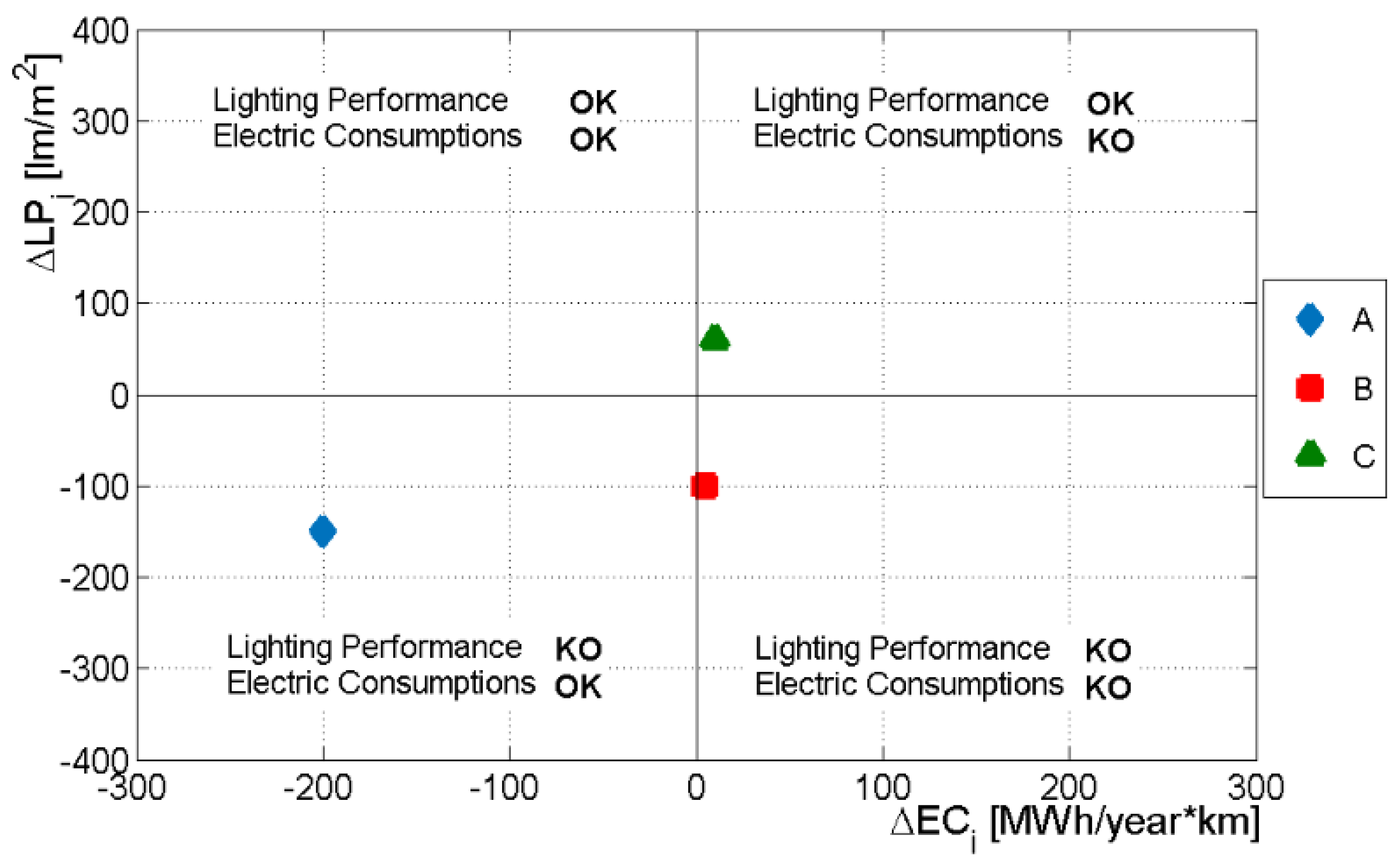
2.3. Intermediate and Final Outputs of EST

Summarizing, the intermediate and final outputs are:

(i)

representation on the same Cartesian plane of all EST, with reference to a set of LSTs, ar the LSTs of interest in the actual state of service;

(ii)

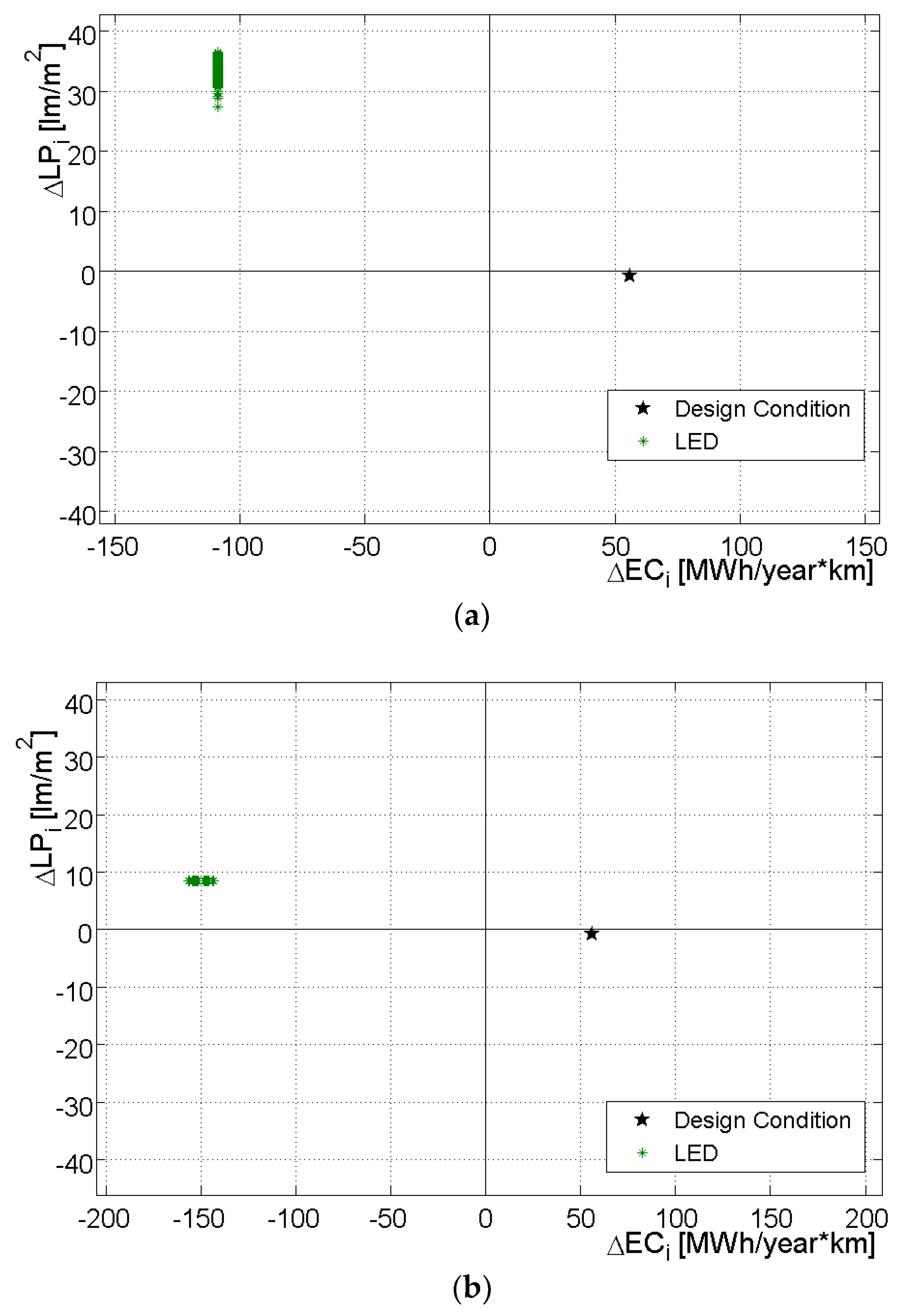
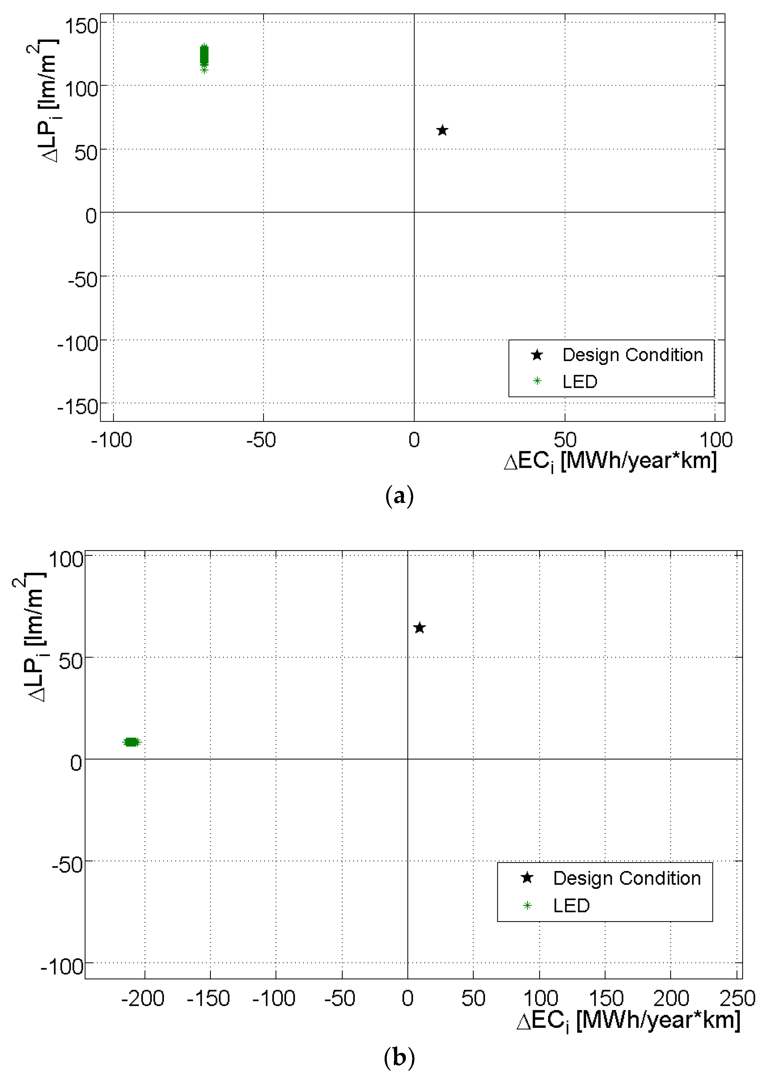
identification on the same Cartesian plane which LST is in an acceptable state of service (second quadrant), which LST needs intervention for reducing the energy consumptions and/or improving the lighting performance;

(iii)

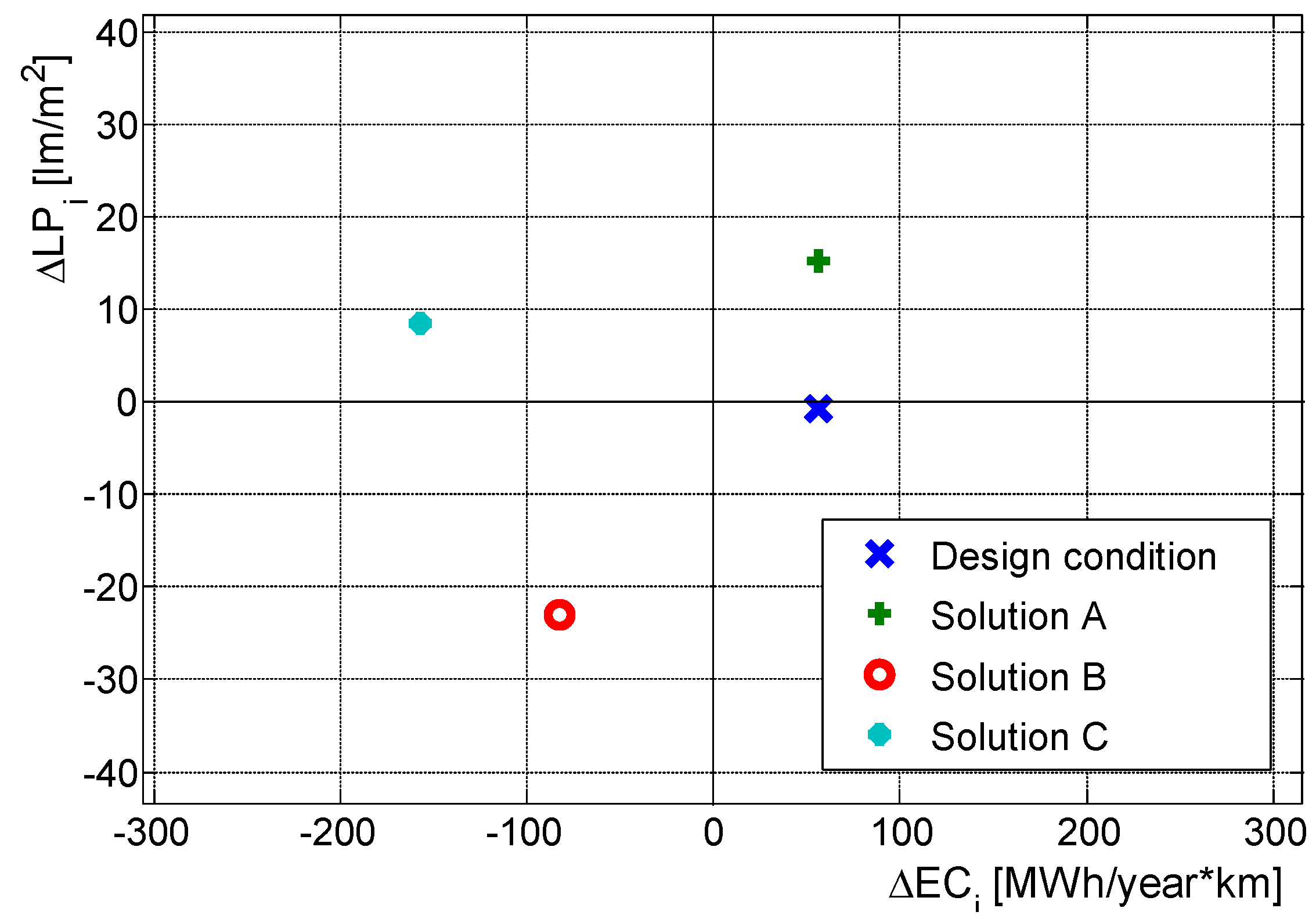
representation on the same Cartesian plane of the effect of the interventions on every LST adopting one of the possible alternatives (substituting the luminaries and/or integrating luminosity regulation);

(iv)

economic evaluation of every intervention on each LST;

(v)

sorting of the alternative solutions by means of the economic quantities NPVS_k or PB_k.

It is evident that the decision maker can prioritize the interventions and make the best choice based on business policies and on the available initial capital costs.

3. Probabilistic Energy Screening of Tunnel, PrEST

The decision on the investments both for improving the lighting performance and for reducing the energy consumptions of an existing LST can be taken using EST when all the data of the model are known without uncertainty. In reality, however, several data and many parameters can be uncertain or assigned with a different grade of confidence.

The most adequate way to take into account the uncertainties is to express the input data by random variables and to apply probabilistic techniques of analysis. In the following, we first analyze the most important EST input data and parameters that require the introduction of random variables. Then, we describe the probabilistic analysis technique.

3.1. Lamp and Luminaires

When we deal with the installation of devices one parameter is strongly uncertain: the useful life. This is particularly true when the devices are characterized by significant technological innovation, as is the case of the luminaires with the solid state lamps like the LEDs [14,15,16]. The value of life influences the annual cost of any solution, and therefore both the economic quantities in Equations (10) and (23).

The “standard” or “default” useful life of a lamp depends on its technology [17]. For all the lamps with the exception of the LED, the useful life is a number of hours of operation at which half the product population, B₅₀, fails; it is the median life of the lamps.

For the LEDs, it was defined in terms of lumen output and specified as the time when light output of half the product population, B₅₀, has fallen below 70% of average initial light output, L₇₀, for any reason [18]. For some applications, also the colour shift of the LED may be considered a failure. For these cases, the lifetime can consider also when light output of half the product population B₅₀ has shifted colour beyond a specified limit that depends on the needs of the specific application.

Reference [19] proposed a life prediction methodology for L₇₀ life of LEDs based on the Kalman filter and the extended Kalman filter models. Both the proposed models were able to predict the lumen degradation as well as the chromaticity shift. It is interesting to evidence that the estimated mean value of L₇₀ for the considered LEDs ranged from about 26,000 to about 40,000 h depending on the underlying degradation mechanism. The standard deviation ranged from about 6% to about 30% of the mean value. Such a large variation of the LED life surely has a large impact on the evaluation of the investments.

A further variable that can be affected by uncertainty is the luminous efficacy, ε, of the lamp and luminaire. This is valid both for the existing devices and for those to install for upgrading the LST.

The luminous efficacy (lm/Watt) is the ratio between the lumens associated with a given optical power, that is the integral of eye response V(λ) over wavelength, and the electrical source power (pe) used to create the optical power:

$$\mathsf{\epsilon }=\frac{\int {\mathrm{p}}_{\mathrm{o}}\left(\mathsf{\lambda }\right)\mathrm{V}\left(\mathsf{\lambda }\right)\mathrm{d}\mathsf{\lambda }}{{\mathrm{p}}_{\mathrm{e}}}$$

(24)

The luminous efficacy in Equation (24) is linked to the efficiency of all the subsystems or components which collectively make up the luminaire. In [20], the luminous efficacy of a warm-white LED luminaire was linked to the thermal efficiency droop, the efficiency of the driver, of the fixture/optical, of the overall luminaire. In particular, for the real value of the luminous efficacy, the operating temperature of the LED package is critical and is variable, for a given thermal design of a luminaire, mainly with the ambient temperature and with the operating current.

These quantities are typically not known with precision at the stage of the planning of the investments for upgrading existing LSTs, even if they were, they would be variable during the time in service of the new LSTs. On the other hand, just the variation along the time of the lumen output is the basis of the definition of the standard useful life L₇₀ of the LEDs, as mentioned above.

3.2. Economic Data and Parameters

The economic parameters α and β in Equations (10) and (23) are affected by the typical uncertainty linked to the estimation over a long time, for example, 20 years, needed to appreciate an investment. Moreover, also the price of the devices to install during the period of N years can vary with time. This variation certainly influences the maintenance costs to face for substituting the components along the time of the study.

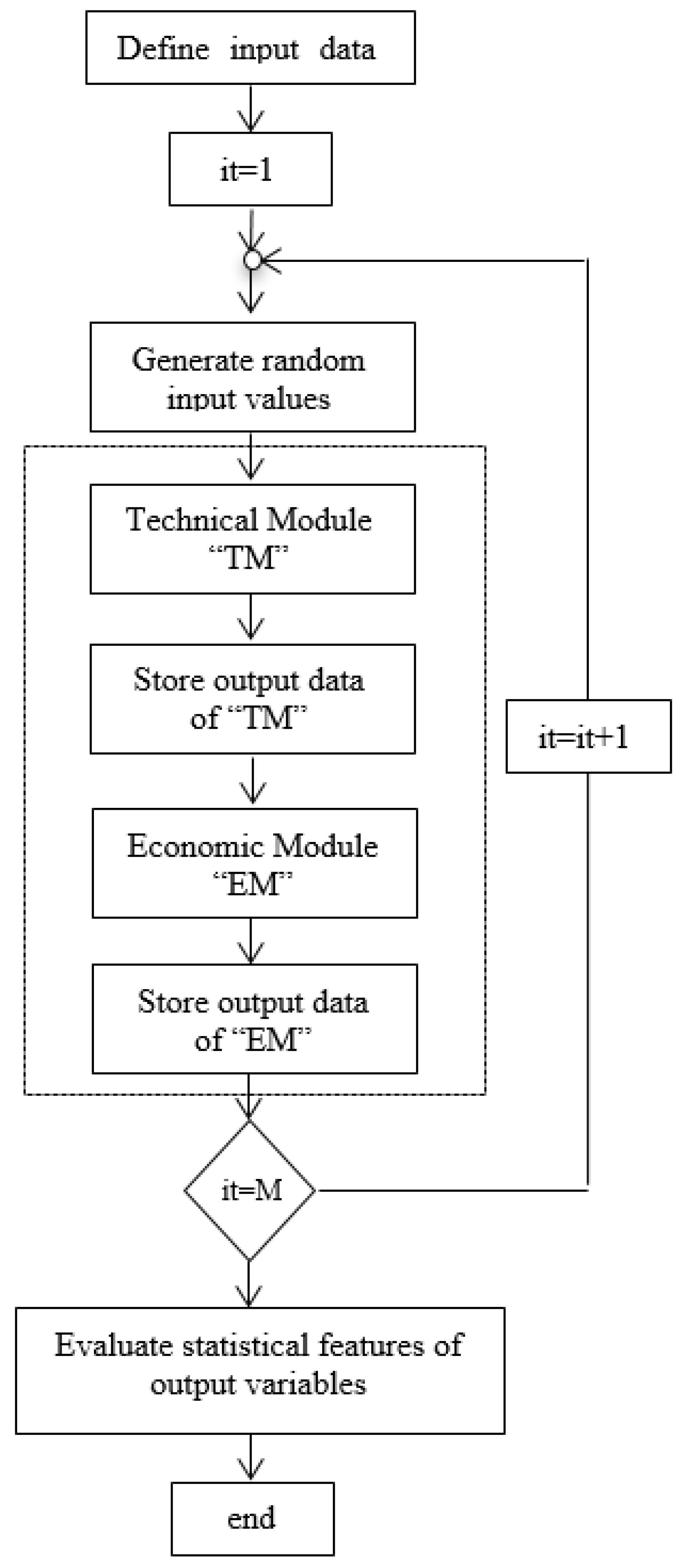
3.3. Probabilistic Analysis Technique

To face the main uncertainties above recalled, the EST model requires to be extended on a probabilistic ground. Given the typology of the EST model, which is not a closed model type, the most adequate technique is the Monte Carlo procedure (Figure 5).

For every LST_i in the study, and for each random input datum, as described in Section 3.1 and Section 3.2, a value is generated according to its proper probability density function (PDF). According to these values, the TM computes the variation indices by Equations (1) and (2). TM performs the technical analysis iteratively for every alternative k.

Once obtained the output values of the TM, they are stored, but each step of simulation does not stop since it continues with the EM to obtain the value of PB_k and NPVS_k by means of the Equations (10) and (23). Once computed PB_k and NPVS_k are stored.

The preceding procedure is repeated a sufficient number (M) of times to obtain a good estimate of the probability of the output variables according to a stated accuracy. The minimum number M* of M can be obtained following the rules in [21].

The previously described Monte Carlo procedure (Figure 5) gives at each step, for every LST_i, the following quantities:

-

by the TM: ∆EC_i and ∆LP_i, computed by Equations (1) and (2), respectively,

-

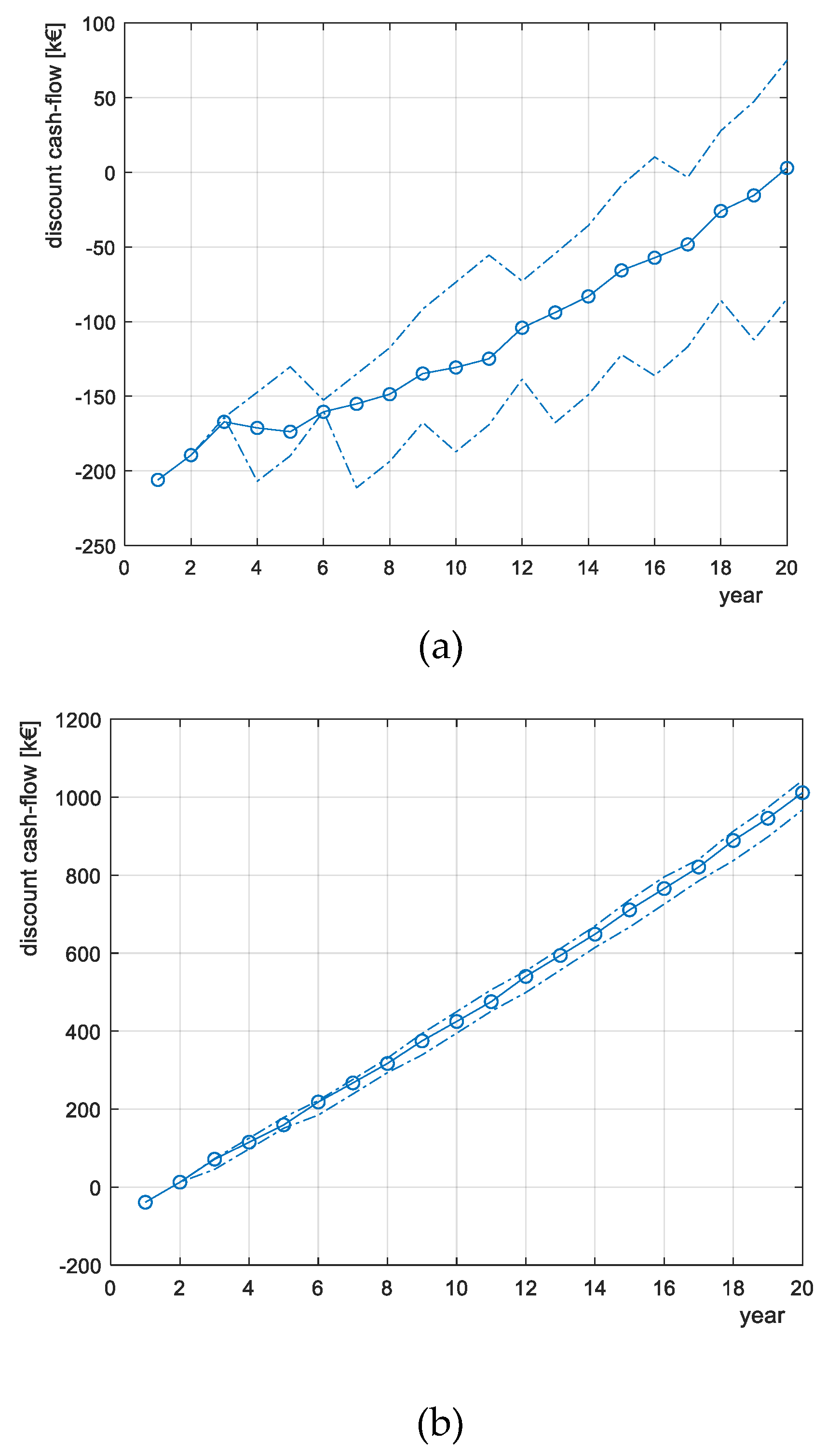
by the EM: NPVS_k and PB_k, computed by the Equations (10) and (23), respectively.

At the end of the M iterations, we obtained the probabilistic characterization of the aforementioned quantities, that is:

-

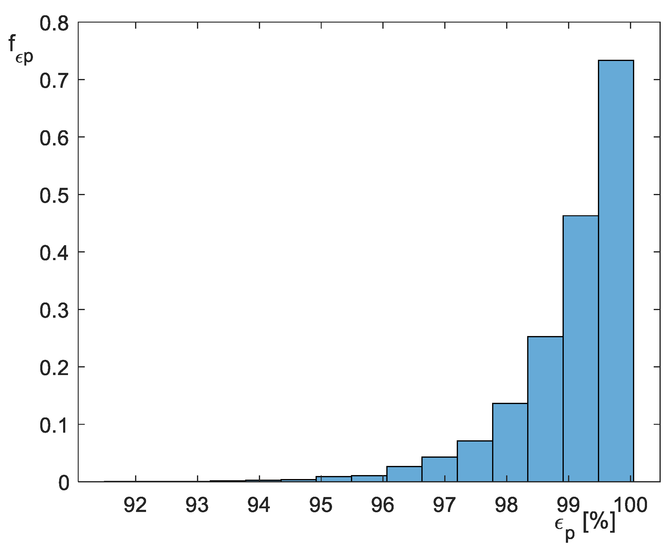
${\mathrm{PDF}}_{{\mathsf{\Delta }\mathrm{EC}}_{\mathrm{i}}}$, the probability density function of the variation index of the annual energy consumption, ∆EC_i;

-

${\mathrm{PDF}}_{{\mathsf{\Delta }\mathrm{LP}}_{\mathrm{i}}}$, the probability density function of the lighting performance, ∆LP_i;

-

${\mathrm{PDF}}_{{\mathrm{NPVS}}_{\mathrm{k}}}$, the probability density function of the present worth of the total savings, NPVS_k;

-

${\mathrm{PDF}}_{{\mathrm{PB}}_{\mathrm{k}}}$, the probability density function of the pay-back period, PB_k.

From the computed PDFs, several statistical features can be used to take the final decision. The decision maker, in fact, can choose the investments for the solution k* that minimizes the mean value of NPVS_k or of a certain percentile Px (NPVS_k), like for example the 95th percentile, P₉₅ (NPVS_k). Similar reasoning can be applied to PB_k. PrEST can be also an adequate tool for performing a sensitivity analysis of the final and intermediate results of TM and EM to the variation and/or the uncertainty of the input data.

4. Numerical Applications on Real Tunnels

PrEST was applied to analyze different solutions for upgrading the lighting system of two real road tunnels whose main characteristics are reported in

Table 1. Main characteristics of the considered road tunnels.

Name	Length [m]	Speed [Km/h]	Type of Road			Actual Lighting Solution
			Number of Carriageways	Number of Directions	Number of Lanes in Each Direction	Permanent	Reinforcement	εp [lm/W]
Tunnel 1	445.8	80	l	2	1	40 SHP 150 W	62 SHP 400 W	95
Tunnel 2	1472.0	70	1	2	1	234 SHP 150 W	98 SHP 400W	120

.

Three different solutions for the new LST have been considered for both road tunnels, as described in the following. All the solutions consider devices available on the actual market:

Solution (A) Substitute new SHP for the existent lamps; in respect to the existent lamps, the new SHP have the same power (150 W for the permanent lamps and 400 W for the reinforcement lamps) and greater efficiency (ε_p = 113 lm/W for the 150 W SHP lamps and ε_p = 135 lm/W for the 400 W SHP lamps). This solution represents a very common choice for which the existent lamps are replaced with lamps of the same technology, with the same power and increased efficiency.

Solution (B) Substitute new SHP for the existent lamps; in respect to the existent lamps, the new SHP have lower power (100 W for the permanent lamps and 250 W for the reinforcement lamps) and greater efficiency (ε_p = 105 lm/W for the 100 W SHP lamp and ε_p = 128 lm/W for the 250 W SHP lamp). This solution represents a possible design result for which the existent lamps are replaced with lamps of the same technology with lower power and increased efficiency.

Solution (C) Substitute LED lamps for the existent lamps; the LED have a power of 150 W and efficiency _p, equal to 137 lm/W both for the permanent and the reinforcement lamps. This solution represents a possible design result for which the existent lamps are replaced with new lamps of different technology.

The economic analysis was conducted with the following assumptions: for all the new solutions, we considered the cost of the lamps, the cost of the lamp substitution, while we neglected the cost of all the other materials. All the costs were derived from commercial public information and from [22,23]. For the LEDs, we supposed that the price of acquisition linearly decreases from the 10th year on. Moreover, we assumed the tariff of the energy at the first year, T₁, equal to 0.167 €/kWh, the variation rate of the energy cost, equal to 0.015, and the rate of return, equal to 0.005.

Firstly, the TM of EST was applied for representing every new solution of the LST in the Cartesian plane {electricity consumption, performance}. Figure 6 and Figure 7 show the results for the Tunnel 1 and Tunnel 2, respectively.

Figure 6 and Figure 7 show that the Solutions (A) and (B), for the Tunnel 1, and the solution (A), for the Tunnel 2, are not acceptable since they do not fall in the second quadrant where both the energy consumptions and the lighting performance are acceptable. The acceptability of the Solutions (C) for the Tunnel 1, and of Solutions (B) and (C) for the Tunnel 2, means that the obtained performance of illumination (and of energy consumptions) are not lower (not greater) than the corresponding performance of illumination (and of energy consumptions) of the baseline case, LST*, of the Tunnel 1 and of the Tunnel 2, respectively. Once selected the new LST solutions, PrEST was applied with M = 10,000 trials considering as input random variables, separately:

(i)

the efficiency of the lamps;

(ii)

the life of the lamps.

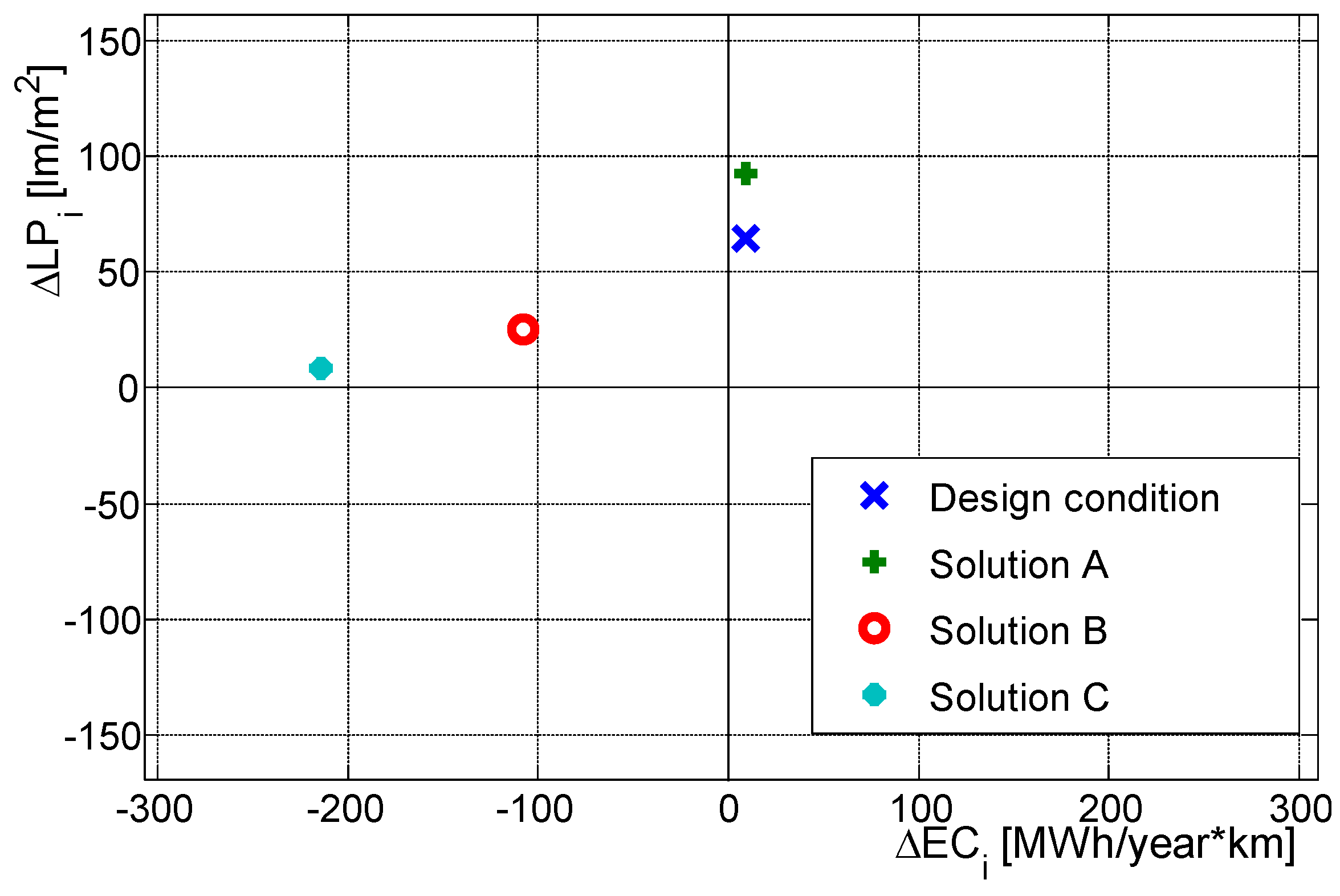
With reference to (i), for considering the unavoidable reduction of the lamp efficiency during the life, we used the asymmetric PDF represented in Figure 8 which is characterized by a maximum value coincident with the nominal efficiency.

With reference to (ii), for considering the uncertainty of the knowledge of the life of the lamps, we used the uniform PDF with the maximum value equal to the nominal value (25,000 h for the SHP and 50,000 h for the LED, respectively) and the minimum value equal to the 50% of the nominal value. Given the acceptable solutions for each tunnel, i.e., Solutions (C) for the Tunnel 1, and Solutions (B) and (C) for the Tunnel 2, in terms of technology (SHP or LED), power and nominal efficiency, we applied the Monte Carlo to two possible scenarios which were different for the number of luminaires equipped with the new lamps; they are:

(a)

number of luminaires equipped with lamps equal to those currently installed (design condition—D.C.); this is a common case in which the new LST uses the same structure and the same lamp positioning of the existing LST;

(b)

number of luminaires equipped with lamps obtained by means of an adaptive procedure (A.P.) that allows for installing the minimum number of luminaires equipped with lamps which guarantees, for the nominal value of efficiency, the location of the LST in the second quadrant of the Cartesian plane {electricity consumption, performance}; this is a case in which a design activity, separated from PrEST, defines a structure and a positioning of the luminaires equipped with lamps different from the existing LST.

As an example of the obtainable results, Figure 9 and Figure 10 show the new LSTs realized with LED in the Cartesian plane for the number of the lamps obtained both in the case D.C. and in the case A.P., for Tunnel 1 and Tunnel 2, respectively. The figures show that all the trials fall in the second quadrant where both the energy consumptions and the lighting performance are acceptable. The index ∆LP_i presents an appreciable dispersion of the values around the mean value (about 23% for the Tunnel 1, and about 12% for the Tunnel 2) when the lamp efficiency is the input random variable (Figure 9a and Figure 10a) and the number of the lamps corresponds to the D.C.; the index ∆EC_i, instead, presents, a less pronounced dispersion of the values (about 9% for the Tunnel 1, and about 4% for the Tunnel 2) when the lamp life is the input random variable (Figure 9b and Figure 10b) and the number of the lamps corresponds to the A.P. For the cases shown in Figure 9 and Figure 10,

Table 2. Results of the economic module of the PrEST model for Tunnel 1 considering the efficiency lamp as a random variable.

Solution	Number of Lamps	$\begin{array}{c}{\mathsf{\mu }}_{\mathbf{NPVS}}\\ \left[\mathbf{k}\mathsf{€}\right]\end{array}$	NPVS Percentile [k€]		${\mathsf{\mu }}_{\mathbf{P}\mathbf{B}}\left[\mathbf{Year}\right]$	PB Percentile [Year]
			5th	95th		5th	95th
C	D.C.	143.1	143.1	143.1	7.5	7.5	7.5

,

Table 3. Results of the economic module of the PrEST model for Tunnel 1 considering the life of lamp as a random variable.

Solution	Number of Lamps	${\mathsf{\mu }}_{\mathbf{N}\mathbf{P}\mathbf{V}\mathbf{S}}\left[\mathbf{k}\mathsf{€}\right]$	NPVS Percentile [k€]		${\mathsf{\mu }}_{\mathbf{P}\mathbf{B}}\left[\mathbf{Year}\right]$	PB Percentile [Year]
			5th	95th		5th	95th
C	D.C.	130.5	104.9	150.1	7	6.5	9.5
	A.P.	224.6	206.4	240.0	3.9	3.5	4.5

,

Table 4. Results of the economic module of the PrEST model for Tunnel 2 considering the efficiency lamp as a random variable.

Solution	Number of Lamps	${\mathsf{\mu }}_{\mathbf{N}\mathbf{P}\mathbf{V}\mathbf{S}}\left[\mathbf{k}\mathsf{€}\right]$	NPVS Percentile [k€]		${\mathsf{\mu }}_{\mathbf{P}\mathbf{B}}\left[\mathbf{Year}\right]$	PB Percentile [Year]
			5th	95th		5th	95th
B	D.C.	591.3	591.3	591.3	1	1	1
C	D.C.	71.4	71.4	71.4	15.5	15.5	15.5

and

Table 5. Results of the economic module of the PrEST model for Tunnel 2 considering the life of lamp as a random variable.

Solution	Number of Lamps	${\mathsf{\mu }}_{\mathbf{N}\mathbf{P}\mathbf{V}\mathbf{S}}\left[\mathbf{k}\mathsf{€}\right]$	NPVS Percentile [k€]		${\mathsf{\mu }}_{\mathbf{P}\mathbf{B}}\left[\mathbf{Year}\right]$	PB Percentile [Year]
			5th	95th		5th	95th
B	D.C.	566.9	528.6	592.2	1	1	1
	A.P.	746.9	713.7	767.6	1	1	1
C	D.C.	2.5	−84.6	75.0	19.4	15.5	>20
	A.P.	1011	967.5	1043	1.5	1.5	1.5

give the corresponding mean value, the 5th and the 95th percentile values of the NPVS and the PB obtained by the EM. In particular, Table 2 and Table 3 report the results obtained for the Tunnel 1 when the input random variable was the lamp efficiency and the life of the lamps, respectively; Table 3 and Table 4 report the results obtained for the Tunnel 2 when the input random variable was the lamp efficiency and the life of the lamps, respectively.

Figure 11 illustrates the plots of the discounted cash flow computed at the end of every year of the study period for the Tunnel 2 in two of the examined cases as an example of additional results obtainable by PrEST. The plots can provide the value of NPVS over a time period shorter than 20 years considered in this study.

5. Discussion

The results in the tables and in the figures shown above allow appreciating the effects of the randomness assumed for selected input variables on the economical outputs of the alternative interventions considered.

First of all, the considered randomness of the efficiency of the lamps (Table 2 and Table 4) does not greatly impact on the dispersion of the output economical indices NPVS and PB. This outcome confirms that any reduction of the efficiency of the lamps impacts only on the lighting performance. In fact, Figure 9a and Figure 10a showed that the spread only affects the index ∆LPI_i, leaving all the points always in the second quadrant. In such conditions, the economic indices NPVS and PB vary slightly.

The effect of the randomness of the life of the lamps, instead, can affect significantly the economic indices (Table 3 and Table 5). In particular, the results of Table 5 related to the case when the LED lamps are replaced using a number of new lamps equal to the existing ones (case D.C.) are particularly interesting. In this case, we obtained not only a low mean value of NPVS (${\mathsf{\mu }}_{\mathrm{NPVS}}$ = 2.5 k€) but also the extreme values of the percentiles very far from it. The P₅ (NPVS) is negative, meaning that in the observation period of 20 years the total investments can be not recovered, even if with a very low probability.

In the literature, the papers dealing with the analysis of the investments on a long period, like for example [5,7], recognized the economic impact of the costs for substituting the designed devices to install at the end of their life. However, in [5], the study considered only the costs of the ordinary maintenance without evaluating the breakdown maintenance. Further in [7], from one hand, the authors gave the range of variation of the expected life of the considered lamps, both for HPS lamps and for LEDs, but, from the other, the economic analysis was performed on a return period corresponding to the service life of the tunnel lighting system, compatible with the lifespan of LED sources, assumed invariant. In other words, the economic analysis ends before the lighting devices get substituted.

The novelty of this model is that it not only allowed accounting for the uncertainty of the expected life of the lamps but it also provided different values of percentiles of the financial indices which, in turn, quantified the incidence of the expected life assumed as random input variable.

The plot of the discounted cash flow computed at the end of every year of the study period shown in Figure 11a proves the widespread of possible economic performance. The difference between the best case (plot of the 95th percentile) and the worst case (plot of the 5th percentile) is really huge. This result is mainly linked to the need of replacing more times the lamps during the 20 years of observation. Obviously, this large impact of the randomness of the lamp life is present also on the index PB. The numerical quantification of the effects of the randomness of the life of the lamps on the financial indices, and on their statistics, give additional valuable information to the decision maker, not derivable from average values of the expected life of lamps assumed invariant.

With reference to the considered scenarios, the NPVS and PB values obtained with the A.P. procedure (new number of lamps defined for obtaining an acceptable lighting performance compared with the baseline case) are generally better than those obtained with D.C. This is motivated by the fact that the application of the adaptive procedure can detect a number of lamps lower than the number of the lamps of D.C.; consequently, with the A.P. both the investment and the running costs are reduced, also overcoming the increase of maintenance costs due to the anticipated substitution of the lamps.

The outcomes obtained, in particular with regards to the random life of the lamps, are very remarkable, and merit verification in more scenarios and in more cases. From the cases considered in this study, as a general consideration we can affirm that replacing the existing lamps with new LED lamps could produce unexpected bad economic results if the life of the installed lamps can be also randomly lower than the nominal one. This, in turn, stresses the need to select new lamps with LED technology characterized by a more stringent guarantee by the production company on the expected life.

As a final comment on the usefulness of the obtainable results by PrEST, the considered economic indices, their statistics together with the available initial investment will support the decision maker for the final choice in function of the business strategy. For example, in function of the selected financial indices, the investments on the Tunnel 1 and on the Tunnel 2 can be sorted. If the objective was to maximize the NPVS, the selection could be to start with the Tunnel 2, analyzing in a second step which solution merit to be properly designed in function of the further financial index PB. For minimizing the PB period, the best choice for Tunnel 2 would be in any case to install new SHPs.

6. Conclusions

The paper deals with decision making on the lighting systems of road tunnels. The proposed approach, PrEST, allows for accounting both the technical performances and the economic objectives of new installations on existing road tunnels in a probabilistic frame in which some parameters are affected by uncertainty.

The results obtained on two real road tunnels prove that some choices, adequate when all the problem data and parameters are deterministic, can result in unacceptable economic outcomes. In some of the considered cases, the uncertainty of the life of the lamps can subvert the expectations of the initial investments. The efficiency of the new lamps, instead, does not greatly affect the final economic results.

PrEST can give different statistics of the economic indices, like the mean value, the 5th and 95th percentiles for providing different grades of confidence to the decision maker. Further studies are in progress for considering additional input random variables, and for including improved characterization of the input random variables.

References

1. Bullough, J.D.; Zhang, X.; Skinner, N.P.; Rea, M.S. Design and Evaluation of Effective Crosswalk Illumination. In PDF FHWA-NJ-2009-03 [Report to the New Jersey Department of Transportation]; New Jersey Department of Transportation: Trenton, NJ, USA, 2009. [Google Scholar]
2. UNI 11095. Light and Lighting: Tunnel Lighting; UNI Unification Italian Committee: Italy, 2003. [Google Scholar]
3. Ying, Y. Study on the Computing Method of Luminance of Tunnel Threshold Zone; Chongqing University: Chongqing, China, 2008. [Google Scholar]
4. Li, F.; Chen, D.; Song, X.; Chen, Y. LEDs: A Promising Energy-Saving Light Source for Road Lighting. In Proceedings of the Power and Energy Engineering Conference, APFEEC 2009, Wuhan, China, 28–31 March 2009. [Google Scholar]
5. Salata, F.; Golasi, I.; Bombelli, E.; de Lieto Vollaro, E.; Nardecchia, F.; Pagliaro, F.; Gugliermetti, F.; de Lieto Vollaro, A. Case Study on Economic Return on Investments for Safety and Emergency Lighting in Road Tunnels. Sustainability 2015, 7, 9809–9822. [Google Scholar] [CrossRef] [Green Version]
6. Parise, G.; Martirano, L.; Parise, L. The energetic impact of the lighting system in the road tunnels. In Proceedings of the 2015 IEEE/IAS 51st Industrial & Commercial Power Systems Technical Conference (I&CPS), Calgary, AB, Canada, 5–8 May 2015; pp. 1–7. [Google Scholar]
7. Salata, F.; Golasi, I.; Bovenzi, S.; Vollaro, E.L.; Pagliaro, F.; Cellucci, L.; Coppi, M.; Gugliermetti, F.; Vollaro, A.L. Energy Optimization of Road Tunnel Lighting Systems. Sustainability 2015, 7, 9664–9680. [Google Scholar] [CrossRef] [Green Version]
8. Caporaso, F.; Montecuollo, M.; Verde, P.; Varilone, P. Energy Savings and Performance Modelling of Tunnel Lighting Systems for Decision Making of Investments. World Road Assoc.–PIARC 2015, 366, 82–87. [Google Scholar]
9. Varilone, P.; Verde, P.; Caporaso, F.; Cesolini, E.; Drusin, S. Integrated modelling and experimental verification of energy consumption and performance of the lighting systems of tunnels. In Proceedings of the AEIT Annual Conference, Trieste, Italy, 18–19 September 2014. [Google Scholar]
10. ARERA, Resolution EEN 4/11, 5 Maggio 2011. Available online: www.arera.it/it/docs/11/004-11een.htm (accessed on 1 February 2019).
11. Energy Efficient Lighting. Available online: www.ncsl.org/research/energy/energy-efficient-lighting.aspx (accessed on 1 February 2019).
12. Free Software Dialux. Available online: https:// dial.de/en/ (accessed on 1 February 2019).
13. International Commission on Illumination. Available online: www.cie.co.at (accessed on 1 February 2019).
14. Luo, D.; Chen, Q.; Gao, Y.; Zhang, M.; Liu, B. Extremely Simplified, High-Performance, and Doping-Free White Organic Light-Emitting Diodes Based on a Single Thermally Activated Delayed Fluorescent Emitter. ACS Energy Lett. 2018, 3, 1531–1538. [Google Scholar] [CrossRef]
15. Liu, B.; Nie, H.; Zhou, X.; Hu, S.; Luo, D.; Gao, D.; Zou, J.; Xu, M.; Wang, L.; Zhao, Z.; et al. Manipulation of Charge and Exciton Distribution Based on Blue Aggregation-Induced Emission Fluorophors: A Novel Concept to Achieve High-Performance Hybrid White Organic Light-Emitting Diodes. Adv. Funct. Mater. 2016, 26, 776–783. [Google Scholar] [CrossRef]
16. Liu, B.Q.; Wang, L.; Gao, D.Y.; Zou, J.H.; Ning, H.L.; Peng, J.B.; Cao, Y. Extremely high-efficiency and ultrasimplified hybrid white organic light-emitting diodes exploiting double multifunctional blue emitting layers. Light Sci. Appl. 2016, 5, e16137. [Google Scholar] [CrossRef] [PubMed]
17. ANSI/IES RP-16-17, Nomenclature and Definitions for Illuminating Engineering. Available online: https://www.ies.org/standards/definitions/ (accessed on 1 February 2019).
18. Next Generation Lighting Industry Alliance LED Systems Reliability Consortium, Led Luminaire Lifetime: Recommendations for Testing and Reporting, 3rd ed.; Next Gen. Lighting Ind.: Washington, DC, USA, 2014.
19. Lall, P.; Wei, J. Prediction of L70 Life and Assessment of Color Shift for Solid-State Lighting Using Kalman Filter and Extended Kalman Filter-Based Models. IEEE Trans. Device Mater. Reliab. 2015, 15, 54–68. [Google Scholar] [CrossRef]
20. Pattison, P.M.; Hansen, M.; Tsao, J.Y. LED lighting efficacy: Status and directions. C. R. Phys. 2017, 19, 134–145. [Google Scholar] [CrossRef]
21. Papoulis, A. Probability and Statistics; Prentice-Hall: Upper Saddle River, NJ, USA, 1989. [Google Scholar]
22. ANAS (Azienda Nazionale Autonoma Delle Strade). Manutenzione Ordinaria. Available online: https://www.stradeanas.it/sites/default/files/pdf/4.5/MO_LISTINO%20PREZZI%202018.pdf (accessed on 30 January 2019). (In Italian).
23. ANAS (Azienda Nazionale Autonoma Delle Strade). Nuove Costruzioni e Manutenzione Straordinaria. Available online: https://www.stradeanas.it/sites/default/files/pdf/4.5/NC-MS_LISTINO%20PREZZI%202018_REV2.pdf (accessed on 30 January 2019). (In Italian).
Figure 1. Plot of the required luminance L along the longitudinal axis x of the tunnel for different reference speeds [2].
Energies 12 01488 g001
Figure 2. EST with the technical TM, and the Economic Module EM.
Energies 12 01488 g002
Figure 3. Cartesian plan {electricity consumption, performance} with three LSTs represented with a green triangle, red square, and blue rhombus [9].
Energies 12 01488 g003
Figure 4. Cartesian plan {electricity consumption, performance} with the alternative interventions on the LST represented in Figure 3 with the green triangle.
Energies 12 01488 g004
Figure 5. Flow chart of PrEST.
Energies 12 01488 g005
Figure 6. Cartesian plan {electricity consumption, performance} for the considered solutions of the Tunnel 1.
Energies 12 01488 g006
Figure 7. Cartesian plan {electricity consumption, performance} for the considered solutions of the Tunnel 2.
Energies 12 01488 g007
Figure 8. Probability density function of lamp efficiency εp in percentage of the nominal value.
Energies 12 01488 g008
Figure 9. Cartesian plan {electricity consumption, performance} obtained in for LED solutions of the Tunnel 1: (a) number of lamps referred to Design Condition (D.C.) with random efficiency of the lamps, (b) number of lamps obtained by Adaptive Procedure (A.P.) with random life of the lamps.
Energies 12 01488 g009
Figure 10. Cartesian plan {electricity consumption, performance} for LED solutions of the Tunnel 2: (a) number of lamps referred to Design Condition (D.C.) with random efficiency of the lamps, (b) number of lamps obtained by Adaptive Procedure (A.P.) with random life of the lamps.
Energies 12 01488 g010
Figure 11. Mean value, 5th and 95th percentile of the discounted cash-flow computed at the end of every year of the study period in case of led lamps used for Tunnel 2 considering the life of lamp as a random variable and the number of lamps calculated by D.C. (a) and A.P (b).
Energies 12 01488 g011