Distributed Reconciliation in Day-Ahead Wind Power Forecasting

Abstract

With increasing renewable energy generation capacities connected to the power grid, a number of decision-making problems require some form of consistency in the forecasts that are being used as input. In everyday words, one expects that the sum of the power generation forecasts for a set of wind farms is equal to the forecast made directly for the power generation of that portfolio. This forecast reconciliation problem has attracted increased attention in the energy forecasting literature over the last few years. Here, we review the state of the art and its applicability to day-ahead forecasting of wind power generation, in the context of spatial reconciliation. After gathering some observations on the properties of the game-theoretical optimal projection reconciliation approach, we propose to readily rethink it in a distributed setup by using the Alternating Direction Method of Multipliers (ADMM). Three case studies are considered for illustrating the interest and performance of the approach, based on simulated data, the National Renewable Energy Labaratory (NREL) Wind Toolkit dataset, and a dataset for a number of geographically distributed wind farms in Sardinia, Italy.

1. Introduction

Renewable energy generation capacities have been deployed at a sustained pace in many areas over the world, bringing a set of challenges for its integration into power systems and electricity markets. For instance, wind power generating capacity worldwide grew by 10% in 2017 with capacity increasing by 47 GW to reach 515 GW by the end of 2017, and especially in Europe wind has become an important contributor in electricity generation. Wind power provided more than 48% of power generation in 2017 in Denmark, and wind power provides 15% or more of power generated in Ireland, Lithuania, Germany and Spain. Forecasting of power generation at lead times between minutes and days ahead is today seen as of utmost importance for reliable and economical usage of renewable energy generation. The large amounts of data collected at wind farms are also a set of interesting opportunities for development of forecasting methodologies.

Large collections of time series are often naturally structured in a hierarchical or grouped manner. Correspondingly, there can be tens of thousands of individual time series to forecast at the most disaggregated level, plus additional series to forecast at higher levels of aggregation. If all the series at all levels of aggregation are predicted independently, one will lose the consistency among prediction levels. Hierarchical time series (HTS) forecasting has therefore been proposed as a way to reconcile forecasts, e.g., to ensure that the forecasts of the disaggregated series add up to the forecasts of the aggregated series [1]. Reconciliation obviously also comes with the aim to maximize forecast accuracy through some form of forecast combination [2].

Wind farms within a certain region may naturally be seen as integrated into the power system with some form of hierarchy, depending upon the way they are connected through given or multiple substations. Similarly through participation in electricity markets, wind farms may be seen as organized in portfolios, hence also with some form of hierarchy. At the wind farm level, wind power forecasts facilitate participation in energy markets and the scheduling of maintenance work [3]. At a portfolio level, the aggregated wind power forecasts allow maximization of cumulative profits in electricity markets [4]. At a higher aggregated level, transmission system operator may use forecasts for scheduling conventional power units and estimating reserves [5].

So far, wind power forecasting is performed independently for individual wind farms and aggregated levels. This hence means that these forecasts do not satisfy the consistency condition expressed before, i.e., that the sum of the individual forecasts is equal to the forecast for the sum. However, in recent proposals like the hierarchical coordinated dispatch [5], the hierarchical Security Constrained Optimal Power Flow (SCOPF) [6] and the Security Constrained Unit Commitment (SCUC) [7], this consistency is seen as a requirement for the input forecasts. In addition, reconciliation may actually impact forecast accuracy overall, if considering all time series involved (i.e., both individual and aggregated levels), since allowing some form of information exchange among sites of interest [7,8].

In contrast with the limited literature that looked at reconciliation problems in wind power forecasting, mainly for very short lead times, for instance several hours ahead with a resolution of 10–15 min, and hence only using past power observations as input e.g., [7], our contribution involves focusing on reconciliation in day-ahead wind power forecasting. Original wind power forecasts are obtained based on nonlinear regression between the information in Numerical Weather Predictions (NWPs) and observed in wind power generation. Only wind speed forecasts are considered as input for simplicity, though the approach described may readily be applied to more complex setups with additional information being accommodated as input to obtaining the base forecasts, i.e., prior to employing the forecast reconciliation mechanism. For the purpose of this work, another contribution consists in reviewing the state-of-the-art approaches to HTS reconciliation methods, in order to yield a novel classification including Generalized Least Squares (GLS), Minimum Trace (MinT) and Game Theoretic Optimal Projection (GTOP) variants. Finally, the various works in the literature assume that the reconciliation process may be centralized, which obviously goes against current operational practice, where many actors may prefer to rely on a decentralized process. Consequently, we propose a distributed reconciliation method of the GTOP method, hence allowing to implement forecast reconciliation in a decentralized environment and to limit the exchange of confidential information among different agents. Specifically, we eventually describe a constrained GTOP problem which is solved through the Alternating Direction Method of Multipliers (ADMM). To illustrate the applicability of our approach and to examine the performance of the methods, three datasets are used including a simulated dataset, National Renewable Energy Labaratory (NREL) dataset and Sardinia dataset. The first dataset is generated by assuming that wind speed follows a Weibull distribution and wind power curve is a piecewise mapping function from wind speed to wind power output. The second dataset, including wind speed forecasts provided by NWP and wind power outputs modeled by International Electrotechnical Commission (IEC) models, can be accessed online. The third dataset is a real dataset, where wind speed forecasts are provided by a NWP model and the wind power outputs are actual measurements.

The paper is structured as follows. First, Section 2 introduces the HTS framework and the basics of the forecast reconciliation problem. It also provides a review of the state of the art of relevance to the application to day-ahead wind power forecasting. Subsequently in Section 3, we describe our proposal based on the GTOP approach to eventually obtain a distributed approach to forecast reconciliation. Section 4 concentrates on application and case-studies, where those various datasets are used to illustrate the workings and benchmark the performance of our forecast reconciliation approach.

2. Hierarchical Time-Series and Forecast Reconciliation

After introducing our notations and presenting the basics of the forecast reconciliation problem, an overview of the state of the art of relevance to the day-ahead wind power forecasting application is provided. Eventually, the main approaches to forecast reconciliation are introduced.

2.1. The Forecast Reconciliation Problem

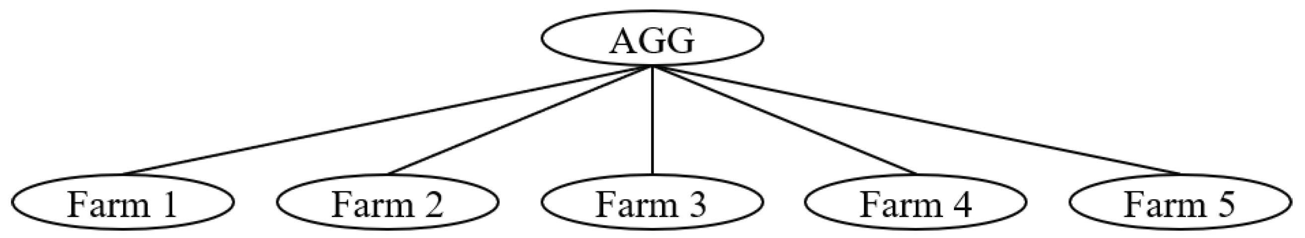
To introduce the notation of the reconciliation problem, we provide an example of wind power forecasting over a region as presented in Figure 1. Figure 1 displays a two-level hierarchy where five nodes at the bottom level correspond to five wind farms and their aggregation is referred to as node “AGG”. The power output of node “AGG” at time t is denoted as $y_{\mathrm{AGG},t}$ and the counterparts of the node at the bottom level is denoted as $y_{k,t}$ for wind farm k, where $k=1,\dots ,5$. The relationship between power measurements at the various wind farms and at the aggregate level naturally is written as

$$\left[\begin{array}{c}{y}_{\mathrm{AGG},t}\\ y_{1,t}\\ y_{2,t}\\ y_{3,t}\\ y_{4,t}\\ y_{5,t}\end{array}\right]=\left[\begin{array}{ccccc}1& 1& 1& 1& 1\\ 1& 0& 0& 0& 0\\ 0& 1& 0& 0& 0\\ 0& 0& 1& 0& 0\\ 0& 0& 0& 1& 0\\ 0& 0& 0& 0& 1\end{array}\right]\left[\begin{array}{c}{y}_{1,t}\\ y_{2,t}\\ y_{3,t}\\ y_{4,t}\\ y_{5,t},\end{array}\right],\forall t.$$

(1)

In a compact form,

$$Y_t=S{Y}_t^b,\forall t.$$

(2)

In the above, S denotes the summation matrix of 1 s and 0 s determined by the hierarchical structure, while $Y_t$ and $Y_t^b$ are the observation vectors formed by all the nodes in the hierarchy and the nodes at the bottom level, respectively. This relationship simply shows that the wind power aggregation at the portfolio or regional level is equal to the summation of the wind farms at the bottom level, which also defines an aggregation consistency constraint for the power measurements also viewed as the aggregation consistency constraint. Hierarchies with more than two levels can also be thought of and considered as in the case of [9,10], though we restrict ourselves here to a two-level case, which is arguably the most relevant one in day-ahead wind power forecasting, for simplicity.

In practice, the aggregation consistency in (2) is satisfied for the actual observations at any time t, while it usually cannot be guaranteed for the case of the base forecasts of all the nodes in the hierarchy which were generated independently. To deal with the aggregate inconsistency problem, reconciliation consists in slightly adjusting the base forecasts to eventually respect the aggregate consistency constraint, hence yielded so-called reconciled forecasts. The aggregation consistency for the reconciled forecasts can be expressed as

$${\tilde{Y}}_{t+h|t}=S{\tilde{Y}}_{t+h|t}^b,\forall t,h,$$

(3)

where ${\tilde{Y}}_{t+h|t}$ and ${\tilde{Y}}_{t+h|t}^b$ are the h-step ahead reconciled forecast vectors made at time t and formed by all the nodes in the hierarchy and the nodes at the bottom level respectively, being consistent with the notations in (2). Likewise, we shall denote the h-step ahead base forecast vector for the hierarchy made at time t as ${\widehat{Y}}_{t+h|t}$ in the following. Possibly counter-intuitively, the process of forecast reconciliation may also yield forecast improvements in the least-squares sense, thanks to some form of information sharing among nodes and aggregation levels.

2.2. An Overview of the State of the Art

In HTS forecasting, the hierarchical relation between multiple time series is exploited to improve the accuracy of the forecasts involved overall. The HTS problem is usually split into two subsequent steps. Firstly, base forecasts for all time series (for $k=1,\dots ,5$ and for the aggregate one in the above example) are performed without worrying about aggregate consistency. Then, a reconciliation procedure is used to obtain the reconciled forecasts following aggregate consistency constraints [11]. Regarding day-ahead wind power forecasting, all the individual base forecasts can be obtained using the information available by the agents involved (e.g., weather forecasts, local meteorological observations, past power measurements) by using any of the available state-of-the-art methods, and then reconciliation approaches can be applied to eventually obtain forecasts that are consistent. A wealth of approaches already exist for generating those base forecasts, combining statistical and physical approaches, in deterministic and probabilistic frameworks, etc. [12,13,14]. This is why we do not describe any specific forecasting method, except in the Appendix A so that interested readers understand how our base forecasts were produced. In contrast, less work exists when it comes to regional power forecasting, or forecasting for aggregate portfolios in general. These few methods include direct aggregation, representative mapping and statistical upscaling [15,16].

Traditional reconciliation methods e.g., bottom up, top-down and middle-out are straightforward to implement, while they fail to utilize all the available information [17]. Apparently, the previously mentioned direct aggregation is identical to bottom-up reconciliation, respecting the coherence constraint, while the aggregated forecast is largely affected by single individual forecasts deviations, especially when wind farms are highly spatially correlated. A Generalized Least Squares (GLS) based optimal reconciliation method for hierarchical time series was proposed, requiring prior knowledge of the covariance matrix of reconciliation forecasts errors that cannot be identified [18]. A GLS reconciled method may simplify to an Ordinary Least Squares (OLS) approach without the need for an estimate of the underlying covariance matrix in [18]. Furthermore, a Minimum Trace (MinT) reconciliation was proposed with the need to estimate the covariance matrix of the base forecast errors (which can be challenging to obtain), with five alternative estimators for that covariance matrix [19]. A Game-Theoretically Optimal (GTOP) reconciliation method was proposed to provide new aggregate consistent forecasts that are guaranteed to be at least as good as the base forecasts in [11]. In detail, when the objective function defined in the GTOP method is to minimize a weighted least squared (WLS) error of all the nodes in the hierarchy under the aggregated consistency constraint, the optimal solution is equal to that of a GLS reconciled method with a diagonal covariance matrix (i.e., the diagonal entries are proportional to their corresponding weight of WLS in the objective function).

Different reconciliation methods were applied in HTS forecasting problems in power systems, for which hierarchies can be formed temporally or spatially. For instance, probabilistic forecasts of wind power in temporal hierarchy are reconciled in [20], improving the accuracy of both point and probabilistic forecasts. A thorough comparison study of all GLS based reconciliation methods on very-short-term wind power forecast was performed in [7] and it validated that reconciled forecasts based on GLS approaches significantly outperform either base forecasts or bottom-up reconciled forecasts. Especially, the MinT reconciliation method appears to yield the highest accuracy in a least squares sense [7]. Reconciliation methods further have also been employed (both temporal and spatial cases) in day-ahead solar power forecasting in [8,21], also showing that MinT reconciliation performs better than other reconciliation methods overall.

2.3. Generalized Least Squares Reconciliation

In a Generalized Least Squares (GLS) reconciliation problem [18], a base forecast can be written as

$${\widehat{Y}}_{t+h|t}=S{\beta }_{t+h|t}+{\mathcal{E}}_{t+h|t},$$

(4)

where ${\beta }_{t+h|t}=\mathbb{E}[Y_{t+h}^b|{\Theta }_t]$ is the h-step-ahead expectation at instant t of the bottom level, and ${\mathcal{E}}_{t+h|t}$ is called the unreconciled error with zero-mean and covariance matrix ${\Sigma }_{t+h|t}$. ${\Theta }_t$ is the information set available at t for the forecast. For instance, it can include weather forecasts, local observations up to time t, etc., for the case of day-ahead wind power forecasting.

This suggests that we can obtain the minimum variance unbiased estimate of ${\beta }_{t+h|t}$ by treating (4) as a regression equation and using GLS estimation as

$${\widehat{\beta }}_{t+h|t}={(S^{\top }{\Sigma }_{t+h|t}^{+}S)}^{-1}{S}^{\top }{\Sigma }_{t+h|t}^{+}{\widehat{Y}}_{t+h|t},$$

(5)

where ${()}^{+}$ is the Moore–Penrose generalized inverse operation [22], and S is the summation matrix formed by the hierarchical structure. This leads to the following reconciled forecasts,

$${\tilde{Y}}_{t+h|t}=S{\widehat{\beta }}_{t+h|t}=S{(S^{\top }{\Sigma }_{t+h|t}^{+}S)}^{-1}{S}^{\top }{\Sigma }_{t+h|t}^{+}{\widehat{Y}}_{t+h|t}.$$

(6)

In the GLS framework, it is often hard to identify the covariance matrix ${\Sigma }_{t+h|t}$ of reconciliation error. In this case, ${\Sigma }_{t+h|t}$ is approximated by an identity matrix of appropriate size and (6) can be reduced to an OLS estimator without the need for an estimate of the underlying covariance matrix, i.e.,

$${\tilde{Y}}_{t+h|t}=S{(S^{\top }S)}^{-1}{S}^{\top }{\widehat{Y}}_{t+h|t}.$$

(7)

2.4. Trace Minimization Reconciliation

Due to the difficulty in obtaining the knowledge of the covariance matrix of the unreconciled error, it is possible to exploit the knowledge of the covariance matrix of base forecast errors instead. For this purpose, let the h-step ahead base and reconciled forecast errors be defined as

$$\begin{array}{cc}\hfill {\widehat{\mathcal{E}}}_{t+h|t}& =Y_{t+h}-{\widehat{Y}}_{t+h|t},\hfill \end{array}$$

(8a)

$$\begin{array}{cc}\hfill {\tilde{\mathcal{E}}}_{t+h|t}& =Y_{t+h}-{\tilde{Y}}_{t+h|t},\hfill \end{array}$$

(8b)

where ${\widehat{Y}}_{t+h|t}$ and ${\tilde{Y}}_{t+h|t}$ are h-step-ahead base and reconciled forecasts using information up to (and including) time t and $Y_{t+h}$ are the observed values of all series at time $t+h$.

Let $W_{t+h|t}$ denote the covariance matrix of the h-step-ahead base forecast error ${\widehat{\mathcal{E}}}_{t+h|t}$. Following Lemma 1 and Theorem 1 described in [18,19], a minimum trace (MinT) reconciliation method provides the best minimum variance linear unbiased reconciled forecasts by minimizing the trace of the reconciled forecast error. The optimal forecasts have a similar expression as (6) where the covariance matrix ${\Sigma }_{t+h|t}$ of the unreconciled errors is replaced by the covariance matrix $W_{t+h|t}$ of the base forecast errors. Specifically,

$${\tilde{Y}}_{t+h|t}=S{(S^{\top }{W}_{t+h|t}^{+}S)}^{-1}{S}^{\top }{W}_{t+h|t}^{+}{\widehat{Y}}_{t+h|t}.$$

(9)

In practice, the covariance matrix $W_{t+h|t}$ of the base forecast errors is estimated based on specific assumptions and available knowledge, as presented in

Table 1. Covariance matrix $W_{t+h|t}$ estimators.

Estimator	Covariance Matrix	Matrix Property
OLS	Identity matrix	diagonal matrix
WLS	$\mathrm{diag}(W_{t+h|t}^e)$	diagonal matrix
HLS	$SI$	full matrix
MinT	$W_{t+h|t}^e$	full matrix
MinT_srk	$\lambda \mathrm{diag}(W_{t+h|t}^e)+(1-\lambda )W_{t+h|t}^e$	full matrix

. According to those alternative estimators listed in Table 1, those rely on an identity matrix of appropriate size, on the empirical estimate of the covariance,

$$W_{t+h|t}^e=\frac{1}{t}\sum _{n=1}^t{\widehat{\mathcal{E}}}_{n+h|n}{\widehat{\mathcal{E}}}_{n+h|n}^{\top },$$

(10)

or on a combination of both. Those alternative approaches are further discussed in the following.

2.4.1. Ordinary Least Squares (OLS) Reconciliation

Here, the simple and special assumption that base forecast errors are independent and identically distributed is used, and then the covariance matrix reduces to

$$W_{t+h|t}^{\mathrm{OLS}}=I$$

(11)

from (9). However, the assumption behind (11) does not usually hold in practical applications of HTS.

2.4.2. Weighted Least Squares (WLS) Reconciliation

Assuming the base forecast errors are uncorrelated, the covariance matrix can be estimated individually as

$$W_{t+h|t}^{\mathrm{WLS}}=\mathrm{diag}(W_{t+h|t}^e).$$

(12)

Accordingly, the WLS reconciled forecasts can be obtained following (9).

2.4.3. Hierarchical Least Squares (HLS) Reconciliation

Assuming the base forecast errors at the bottom level are independent and identically distributed, and the variance of the base forecast of the aggregated node is the summation of all corresponding variances of its leaf nodes, the covariance matrix $W_{t+h|t}^{\mathrm{HLS}}$ can be written as

$$W_{t+h|t}^{\mathrm{HLS}}=SI$$

(13)

where I is the identity matrix. The covariance matrix is independent of both data and forecasting model since no estimation of the covariance matrix is needed [10].

2.4.4. Minimum Trace (MinT) Reconciliation and Shrinkage Estimator

The empirical estimation of the covariance matrix using the information up to (and including) time t is made for MinT reconciliation as

$$W_{t+h|t}^{\mathrm{MinT}}=W_{t+h|t}^e.$$

(14)

In addition, a shrinkage estimator with diagonal target, denoted as MinT_srk, is used whose covariance matrix is

$$W_{t+h|t}^{\mathrm{MinT}\_\mathrm{srk}}=\lambda \mathrm{diag}(W_{t+h|t}^e)+(1-\lambda )W_{t+h|t}^e,$$

(15)

where $\lambda$ ($0<\lambda <1$) is the shrinkage intensity parameter and can be estimated using the method proposed in [23].

3. Proposed Distributed Reconciliation Methods

In this section, the GTOP reconciliation method proposed in [11] is recalled first, and then the relationship between GTOP and WLS (or OLS) reconciliation methods is analyzed, motivating us to propose a distributed way to solve the HTS forecasting problem under the GTOP set-up. Additionally, the parameters and constraints involved in the GTOP set-up are further explored.

3.1. Game Theoretical Optimal (GTOP) Reconciliation

As different assumptions are made for the unreconciled errors and base forecast errors in Section 2, a game-theoretic set-up was proposed to map any given base forecasts to the aggregate consistent forecasts in [11]. To map base forecasts ${\widehat{Y}}_{t+h|t}$ onto aggregate consistent predictions ${\tilde{Y}}_{t+h|t}$, a minimax optimization problem was formulated in [11] as

$$V=\underset{{\tilde{Y}}_{t+h|t}\in \mathcal{A}}{min}\underset{Y_{t+h}\in \mathcal{A}\cap \mathcal{B}}{max}l(Y_{t+h},{\tilde{Y}}_{t+h|t})-l(Y_{t+h},{\widehat{Y}}_{t+h|t}),$$

(16)

where $\mathcal{A}$ indicates the hyperplane determined by the aggregated consistency constraint, $\mathcal{B}$ indicates extra available knowledge on the data, and l represents the loss function. It is observed that the reconciled forecast ${\tilde{Y}}_{t+h|t}$ is selected to guarantee that $l(Y_{t+h},{\tilde{Y}}_{t+h|t})-l(Y_{t+h},{\widehat{Y}}_{t+h|t})$ is at most V regardless of $Y_{t+h}$. Encouragingly, $L_2$-projection displayed in (17) can guarantee that V is below zero if reconciled forecasts ${\tilde{Y}}_{t+h|t}={\tilde{Y}}_{t+h|t}^{\mathrm{GTOP}}$. This implies that we can have at least better forecasts than base forecasts ${\widehat{Y}}_{t+h|t}$. In this case, the reconciled forecasts turn out to be the result from an $L_2$-projection of ${\widehat{Y}}_{t+h|t}$ onto $\mathcal{A}\cap \mathcal{B}$ after scaling all dimensions according to the weight matrix A, i.e.,

$${\tilde{Y}}_{t+h|t}^{\mathrm{GTOP}}=\underset{{\tilde{Y}}_{t+h|t}\in \mathcal{A}\cap \mathcal{B}}{arg\; min}{∥A{\tilde{Y}}_{t+h|t}-A{\widehat{Y}}_{t+h|t}∥}_2^2.$$

(17)

In general, the $L_2$-norm (denoted as ${\parallel \parallel }_2$) of a vector is adopted as loss function, where A is a diagonal matrix accounting for the weighting factors for the weighted errors. In detail, it can be expressed in a summation form in terms of the wind forecast example presented in Section 2.1 as

$${∥A{\tilde{Y}}_{t+h|t}-A{\widehat{Y}}_{t+h|t}∥}_2^2=\sum _{k=1}^K{a}_k{f}_k({\tilde{y}}_{k,t+h|t}-{\widehat{y}}_{k,t+h|t})+a_{\mathrm{AGG}}{f}_{\mathrm{AGG}}({\tilde{y}}_{\mathrm{AGG},t+h|t}-{\widehat{y}}_{\mathrm{AGG},t+h|t}),$$

(18)

where $A=\mathrm{diag}(\sqrt{a_{\mathrm{AGG}}},\sqrt{a_1},\dots ,\sqrt{a_K})$, while $f_k(x)$ and $f_{\mathrm{AGG}}(x)$ are scalar functions such that $f_k(x)=\frac{x^2}{2}$ and $f_{\mathrm{AGG}}(x)=\frac{x^2}{2}$.

A consequence of Theorem 1 in [11] is that a unique projection exists if $\mathcal{B}$ is a closed, convex set and $\mathcal{A}\cap \mathcal{B}$ is not empty. Specifically, if $\mathcal{B}={\mathbb{R}}^K$ (K is the total number of nodes at the bottom level) hence not imposing constraints on the reconciliation, the GTOP forecasts are equivalent to WLS reconciled forecasts. Furthermore, if the weight matrix A is also an identity matrix, GTOP reconciled forecasts are identical to OLS reconciled ones. Therefore, OLS and WLS reconciliation can be generalized as GTOP reconciliation with no extra constraint $\mathcal{B}$.

All the reconciliation methods mentioned above are implemented in a centralized manner. Interestingly, the objective function of GTOP (WLS or OLS) is the summation of a loss function (such as mean square error) for all nodes, which is separable on a node-by-node basis. This readily gives the possibility to reconcile forecasts in a distributed manner using e.g., ADMM, as described in detail in the next subsection. Since our distributed approach based on ADMM to solve the GTOP reconciliation problem requires an extra constraint $\mathcal{B}$, it is further referred as constrained ADMM and denoted as CADMM (WLS-CADMM or OLS-CADMM).

3.2. Constrained GTOP Solved by ADMM

The constrained GTOP problem seen as WLS or OLS problems can be readily solved in a centralized manner [11]. In that case, all information is gathered by a central agent which manages the reconciliation process. However in practice, it is highly likely that wind farm owners and operators would rather not share data or private information, even if that could eventually yield forecast improvements overall. Consequently here, we rethink the GTOP reconciliation problem so as to be solved in a distributed manner. ADMM is a natural candidate approach for distributed optimization allowing to preserve data privacy among all the nodes in the hierarchy, since it only requires sharing of the base forecast errors instead of the actual data.

As the loss function (18) in the GTOP reconciliation method is consistently defined for any lead time h at moment t, where $h=1,\dots ,Ts$ (i.e., $Ts=24$ in day-ahead wind power forecasting), it indicates the reconciliation process is considered and handled individually for any lead time h at moment t, and independently of other times and lead times. Therefore, t and h are ignored in the following in order to lighten notations. The constrained GTOP optimization problem for a two-level hierarchy with K nodes at the bottom level and a single aggregation node can be generally expressed as

$$\begin{array}{cc}\hfill \underset{{\tilde{y}}_1,\dots ,{\tilde{y}}_K}{arg\; min}& \sum _{k=1}^K{a}_k{f}_k({\tilde{y}}_k-{\widehat{y}}_k)+a_{\mathrm{AGG}}{f}_{\mathrm{AGG}}({\tilde{y}}_{\mathrm{AGG}}-{\widehat{y}}_{\mathrm{AGG}})\hfill \end{array}$$

(19a)

$$\begin{array}{cc}\hfill \mathrm{s}.\mathrm{t}.& \sum _{k=1}^K{\tilde{y}}_k={\tilde{y}}_{\mathrm{AGG}}\hfill \end{array}$$

(19b)

$$\begin{array}{cc}\hfill & b_k^{\mathrm{low}}\le {\tilde{y}}_k-{\widehat{y}}_k\le b_k^{\mathrm{up}},k=1,\dots ,K.\hfill \end{array}$$

(19c)

In the above, all f are quadratic loss functions, i.e., $f(ϵ)=\frac{{ϵ}^2}{2}$.

Comparing (19a) to (17), $\tilde{Y}={[{\tilde{y}}_{\mathrm{AGG}},{\tilde{y}}_1,{\tilde{y}}_2,\dots ,{\tilde{y}}_K]}^{\top }$, $\widehat{Y}={[{\widehat{y}}_{\mathrm{AGG}},{\widehat{y}}_1,{\widehat{y}}_2,\dots ,{\widehat{y}}_K]}^{\top }$ and the diagonal weight matrix $A=\mathrm{diag}(\sqrt{a_{\mathrm{AGG}}},\sqrt{a_1},\dots ,\sqrt{a_K})$. Let us write $B^{\mathrm{low}}=[b_1^{\mathrm{low}},b_2^{\mathrm{low}},\dots ,b_K^{\mathrm{low}}]$ and $B^{\mathrm{up}}=[b_1^{\mathrm{up}},b_2^{\mathrm{up}},\dots ,b_K^{\mathrm{up}}]$. The constraints defined by $\mathcal{A}$ and $\mathcal{B}$ are for the aggregated consistency and the boundary constraint in (19c), respectively. If additionally introducing

$$\begin{array}{cc}\hfill \Delta y_k& ={\tilde{y}}_k-{\widehat{y}}_k,k=1,\dots ,K\hfill \end{array}$$

(20a)

$$\begin{array}{cc}\hfill f_k^{\prime }(\Delta y_k)& =a_k{f}_k(\Delta y_k),\mathrm{dom}{f}_k^{\prime }=\{\Delta y_k|b_k^{\mathrm{low}}\le \Delta y_k\le b_k^{\mathrm{up}}\},k=1,\dots ,K\hfill \end{array}$$

(20b)

$$\begin{array}{cc}\hfill g\left(\sum _{k=1}^K\Delta y_k-\Delta \right)& =a_{\mathrm{AGG}}{f}_{\mathrm{AGG}}\left(\sum _{k=1}^K\Delta y_k-\Delta \right),\hfill \end{array}$$

(20c)

then the optimization problem in (19a)–(19c) can be rewritten so as to recognize a sharing problem, i.e.,

$$arg\; min\sum _{k=1}^K{f}_k^{\prime }(\Delta y_k)+g\left(\sum _{k=1}^K\Delta y_k-\Delta \right).$$

(21)

Such a sharing problem can eventually be reformulated as

$$\begin{array}{cc}\hfill arg\; min& \sum _{k=1}^K{f}_k^{\prime }(\Delta y_k)+g\left(\sum _{k=1}^K{z}_k-\Delta \right)\hfill \end{array}$$

(22a)

$$\begin{array}{cc}\hfill \mathrm{s}.\mathrm{t}.& \Delta y_k-z_k=0,k=1,\dots ,K,\hfill \end{array}$$

(22b)

so that ADMM may be readily applied as in [24]. This yields the iterative solving procedure defined, at iteration $i+1$ by the following three update steps,

$$\begin{array}{cc}\hfill \Delta y_k^{i+1}& =\underset{\Delta y_k}{arg\; min}\left(f_k^{\prime }(\Delta y_k)+(\rho /2){∥\Delta y_k-\Delta y_k^i+\Delta {\overline{y}}^i-{\overline{z}}^i+u_k^i∥}^2\right)\hfill \end{array}$$

(23a)

$$\begin{array}{cc}\hfill {\overline{z}}^{i+1}& =\underset{\overline{z}}{arg\; min}\left(g(K\overline{z}-\Delta )+(K\rho /2){∥\overline{z}-\Delta {\overline{y}}^{i+1}-u^i∥}^2\right)\hfill \end{array}$$

(23b)

$$\begin{array}{cc}\hfill u^{i+1}& =u^i+\Delta {\overline{y}}^{i+1}-{\overline{z}}^{i+1}.\hfill \end{array}$$

(23c)

where $\overline{z}=\frac{1}{K}{\sum }_{k=1}^K{z}_k$, $\Delta \overline{y}=\frac{1}{K}{\sum }_{k=1}^K\Delta y_k$. In the present case it eventually simplifies to

$$\begin{array}{cc}\hfill \Delta y_k^{i+1}& =t{h}_k({(a_k+\rho )}^{-1}\rho (\Delta y_k^i-\Delta {\overline{y}}^i+{\overline{z}}^i-u_k^i))\hfill \end{array}$$

(24a)

$$\begin{array}{cc}\hfill {\overline{z}}^{i+1}& ={(K{a}_{\mathrm{AGG}}+\rho )}^{-1}\left(\rho (\Delta {\overline{y}}^{i+1}+u^i)+a_{\mathrm{AGG}}\Delta \right)\hfill \end{array}$$

(24b)

The domain of (23a) is determined by the boundary constraints, described as an element-wise threshold function $t{h}_k(z)$ that

$$t{h}_k(z)=\left\{\begin{array}{cc}{b}_k^{\mathrm{low}}\hfill & z\le b_k^{\mathrm{low}}\hfill \\ z\hfill & b_k^{\mathrm{low}}\le z\le b_k^{\mathrm{up}}\hfill \\ b_k^{\mathrm{up}}\hfill & b_k^{\mathrm{up}}\le z\hfill \end{array}\right..$$

(25)

The whole process of solving constrained GTOP problem by ADMM, and its detailed steps, is summarized in Algorithm 1 below.

Algorithm 1 constrained GTOP Algorithm

1: Require: base forecasts $\widehat{Y}={[{\widehat{y}}_{\mathrm{AGG}},{\widehat{y}}_1,{\widehat{y}}_2,\dots ,{\widehat{y}}_K]}^{\top }$; $A=\mathrm{diag}(\sqrt{a_{\mathrm{AGG}}},\sqrt{a_1},\dots ,\sqrt{a_K})$;  2:   aggregated consistency $\mathcal{A}$; boundary constraint $\mathcal{B}:B^{\mathrm{up}},B^{\mathrm{low}}$  3: Input: $\Delta ={\widehat{y}}_{\mathrm{AGG}}-{\sum }_{k=1}^K{\widehat{y}}_k,\Delta y_k^i,{\overline{z}}^i,u^i$  4: Output: reconciled forecasts $\tilde{Y}={[{\tilde{y}}_{\mathrm{AGG}},{\tilde{y}}_1,{\tilde{y}}_2,\dots ,{\tilde{y}}_K]}^{\top }$  5: while stopping criteria do  6:  $\Delta y_k^{i+1}=t{h}_k({(a_k+\rho )}^{-1}\rho (\Delta y_k^i-\Delta {\overline{y}}^i+{\overline{z}}^i-u_k^i))$  7:  ${\overline{z}}^{i+1}={(K{a}_{\mathrm{AGG}}+\rho )}^{-1}\left(\rho (\Delta {\overline{y}}^{i+1}+u^i)+a_{\mathrm{AGG}}\Delta \right)$  8:  $u^{i+1}=u^i+\Delta {\overline{y}}^{i+1}-{\overline{z}}^{i+1}.$  9:  $i=i+1$ 10: end while 11: ${\tilde{y}}_k={\widehat{y}}_k+\Delta y_k$, ${\tilde{y}}_{\mathrm{AGG}}={\sum }_{k=1}^K{\tilde{y}}_k$

Stopping criteria in step 5 refer to the condition such that both the primal residue $r^i$ and dual residue $s^i$, at iteration i, must be small, i.e.,

$${∥r^i∥}_2\le {ϵ}^{\mathrm{pri}},{∥s^i∥}_2\le {ϵ}^{\mathrm{dual}},$$

(26)

where

$$r^i=\Delta {\overline{y}}^i-{\overline{z}}^i{s}^i={\overline{z}}^i-{\overline{z}}^{i-1},$$

(27)

and ${ϵ}^{\mathrm{pri}}$ and ${ϵ}^{\mathrm{dual}}$ are the feasibility tolerances for the primal and dual residues, respectively [24]. They are chosen using an absolute and relative criterion, i.e.,

$$\begin{array}{cc}\hfill {ϵ}^{\mathrm{pri}}& ={ϵ}^{\mathrm{abs}}+{ϵ}^{\mathrm{rel}}\max \left\{{∥{\overline{y}}^i∥}_2,{∥{\overline{z}}^i∥}_2\right\}\hfill \end{array}$$

(28a)

$$\begin{array}{cc}\hfill {ϵ}^{\mathrm{dual}}& ={ϵ}^{\mathrm{abs}}+{ϵ}^{\mathrm{rel}}{∥u^i∥}_2,\hfill \end{array}$$

(28b)

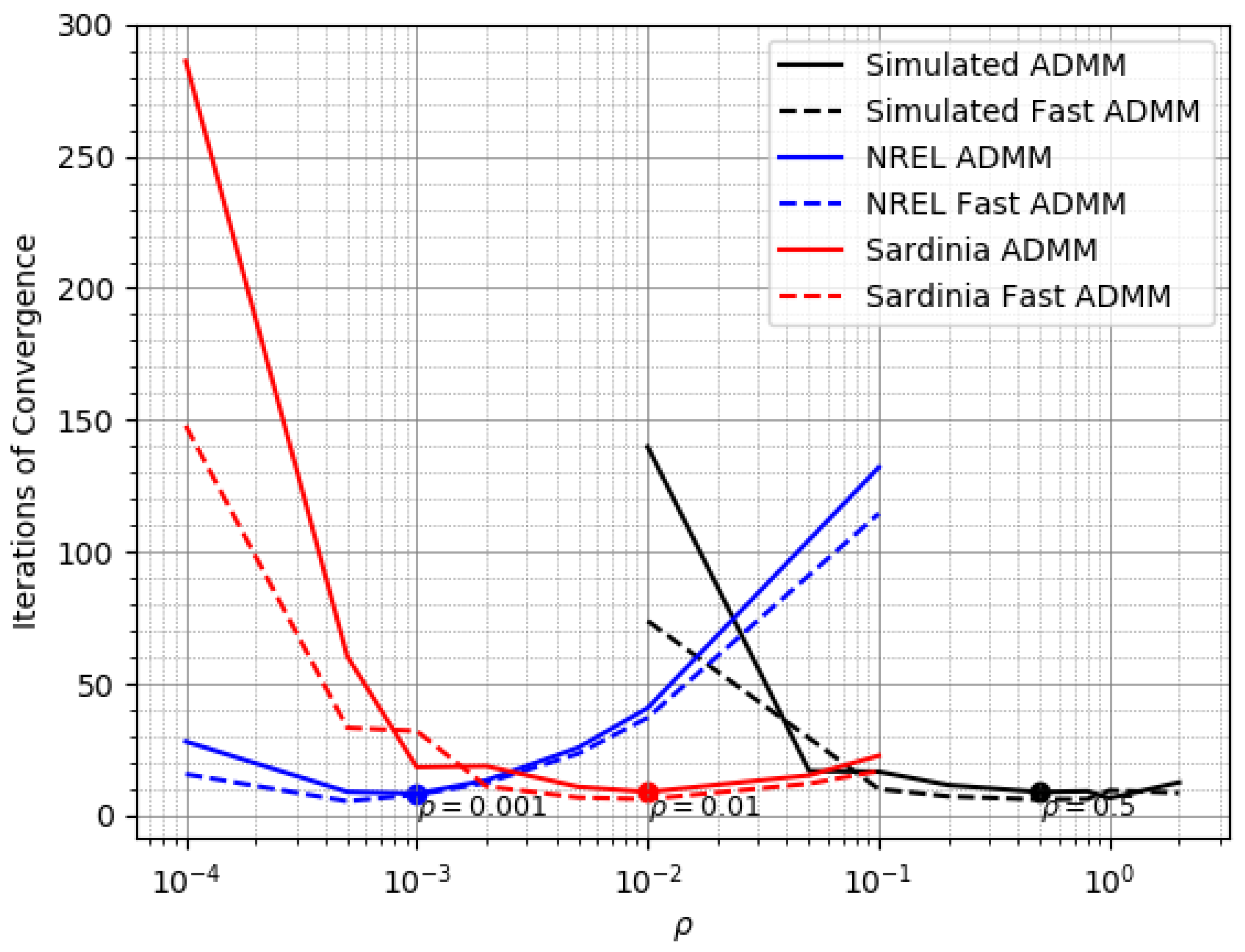
where ${ϵ}^{\mathrm{abs}}>0$ is an absolute tolerance and ${ϵ}^{\mathrm{rel}}>0$ is a relative tolerance. Here, we set both of them to be ${10}^{-3}$. The parameter $\rho$ is fixed for each dataset in our application. Following the steps in Algorithm 1 for our test cases of limited sizes (described in a further part of the present paper), the stopping criteria are satisfied after nine iterations on average. It can be accelerated by using Fast ADMM proposed in [25] with only five iterations required on average. It can be clearly noted in Algorithm 1, the information exchange in step 6 is the base forecast error $\Delta y_k$ (defined in (20a)) for each wind farm k instead of directly sharing the local original history data and independently generated base forecast. This does not only help improve forecast accuracy but also protect data privacy for individual wind farms. This ADMM-based approach to solving a constrained GTOP problem in a two-level hierarchy can be generalized to the case of multiple-level hierarchies as well. The difference lies in the fact that the constrained problem in a two-level hierarchy can be accomplished by one ADMM, while that in a l-level hierarchy needs $(l-1)$ (nested) ADMMs.

3.3. Online Estimate of Individual Variance

In the GTOP reconciliation approach, the selection of a weight matrix A may have an impact on the reconciled results, and finding a reasonable weight matrix is a necessary and challenging task. Fortunately, by comparing the WLS and GTOP approaches, it is observed that the weight matrix $A^{\top }A={\Sigma }^{-1}$ [11]. Thus a reasonable choice of matrix A can be obtained if an estimate of the covariance matrix $\Sigma$ of base forecast errors is available. In practice, prior knowledge of that covariance matrix can be obtained from base forecasts $\widehat{Y}$ and observed data Y, as the base forecast error is assumed to follow a Gaussian distribution with zero mean. The variance of forecasts errors for any node k can be estimated individually and empirically for each node using the information up to and including time t by

$${\sigma }^2=1/t\sum _{n=1}^t{\widehat{e}}_n^2,$$

(29)

where ${\widehat{e}}_n$ is base forecast error at time n. Therefore, this corresponds to the selection that the weight $a_k=1/{\sigma }_k^2$ for node (i.e., wind farm) k at the bottom level. In day-ahead wind power forecasting, the dataset is updated every 24 h, thus updating the variance in the same manner.

3.4. Boundary Constraint

In the GTOP reconciliation problem, the constraints $\mathcal{B}$ may be used to provide extra prior knowledge of $\Delta y_k$, if available, in the form of the interval $[b_k^{\mathrm{low}},b_k^{\mathrm{up}}]$ [11]. The interval of $\Delta y_k$ can also be described as $\left[{\mu }_k+c_k{\sigma }_k,{\mu }_k+d_k{\sigma }_k\right]$ at a certain confidence level using the mean value ${\mu }_k$ and variance ${\sigma }_k^2$ for each node. In base forecast models, the base forecast error is assumed to follow a Gaussian distribution of zero-mean, and thus the expected ${\mu }_k$ is zero, and its variance ${\sigma }_k^2$ can be estimated empirically from (29). Hence, we can further derive a confidence interval

$$b_k^{\mathrm{low}}\le \Delta y_k\le b_k^{\mathrm{up}},\mathrm{i}.\mathrm{e}.,c_k{\sigma }_k\le {\overline{y}}_k-{\widehat{y}}_k\le d_k{\sigma }_k,$$

(30)

where the variance estimate ${\sigma }_k^2$ is obtained according to (29). Empirically, the interquartile is selected as the confidence interval so that $b_k^{\mathrm{low}}$ and $b_k^{\mathrm{up}}$ are 25% and 75% quantiles.

4. Application and Case-Studies

4.1. Framework and Verification

To illustrate the workings and performance of the various reconciliation approaches in day-ahead wind power forecasting, three case studies are considered: (i) On a simulated dataset, (ii) a subset of an NREL dataset, and (iii) a real-world dataset from Sardinia. In all cases, the modelling and forecasting to obtain base forecasts only relies on wind speed to power conversion, where wind speed information originates from weather forecasts. The characteristics and specific features of the three datasets involved are collated in

Table 2. Dataset features.

Dataset	Wind Speeds	Power Output
Simulated dataset	Randomly generated	Simulated
NREL dataset	Provided	Simulated
Sardinia dataset	Provided	Measured

.

In the simulated dataset all wind speed and power outputs of the five wind farms involved are generated following an approach that will be described in the following. For the NREL dataset, we selected the six wind farms located in Kentucky, USA, for which predicted wind speeds and power outputs are provided, though power outputs are not actual observations but simulated instead. The Sardinia dataset covers four wind farms located on the island of Sardinia in Italy, with wind speed forecasts and power measurements at the wind farms being available. The size and setup for those three datasets are comparable since they share a two-level hierarchical structure and the numbers of wind farms at the bottom level are nearly the same. Moreover, data sets cover a period of approximately one year (8784 samples) with a hourly time resolution.

The base forecasts of wind power output are made by using radial basis function based support vector regression (RBFSVR), and more details can be found in Appendix A. The previously mentioned reconciliation methods are employed on those three datasets to examine their performance afterwards. On the simulated dataset, all the reconciliation methods are compared and analyzed. On the latter two datasets, we mainly focus on the performances of GTOPs in a centralized way (WLS or OLS) and in a distributed way (ADMM). All the reconciliation methods listed in Table 1 are used as benchmarks, and the proposed reconciliation method is denoted as CADMM in the following figures and tables. In the implementation of CADMM, the parameter $\rho$ in Algorithm 1 is selected according to specific dataset as presented in Figure 2.

In addition, normalized mean absolute error (NMAE), normalized root mean square error (NRMSE) and improvement of RMSE (IRMSE) are used as indices to present the performance of all the reconciliation methods, where IRMSE of the reconciliation method x can be defined as

$${\mathrm{IRMSE}}_{\mathrm{x}}=\frac{{\mathrm{RMSE}}_{\mathrm{Base}}-{\mathrm{RMSE}}_{\mathrm{x}}}{{\mathrm{RMSE}}_{\mathrm{Base}}}.$$

(31)

Since the loss function defined in GTOP reconciliation problem in (18) is a weighted summation of all the errors between the base forecasts and reconciled forecasts in the whole hierarchy, similarly we propose an overall score to evaluate the performance of the GTOP methods (centralized and distributed). It is defined as the summation of NMSEs (SNMSE) of different levels where the errors are between the actual values and the reconciled forecasts.

$$\mathrm{SNMSE}=\sum _{l=1}^L{\mathrm{NMSE}}_l,$$

(32)

where $NMS{E}_l$ represents the NMSE at level l in a hierarchy of L levels.

4.2. Reconciliation on the Simulated Dataset

A two-level hierarchy of one aggregated node and five distributed nodes representing the wind power aggregation and five wind farms is simulated, as presented in Figure 1. Wind speeds are generated using a Weibull distribution and their corresponding power outputs are generated using a piecewise function in which a cubic function is used to describe the power curve for the wind speed interval determined by the cut-in speed and the rated speed. Wind speeds w are generated following Weibull distribution

$$f(w)=\frac{C}{\eta }{\left(\frac{w}{\eta }\right)}^{C-1}{e}^{{(-\frac{w}{\eta })}^C},$$

(33)

where C is the shape parameter and $\eta$ is the scale parameter [26]. The average wind power output curve is modeled by a piecewise function of four sub-functions as

$$p_{\mathrm{av}}(w)=\left\{\begin{array}{cc}0\hfill & w\le w_{\mathrm{cin}}\hfill \\ C_p{w}^3\hfill & w_{\mathrm{cin}}\le w\le w_r\hfill \\ p_r\hfill & w_r\le w\le w_{\mathrm{cout}}\hfill \\ 0\hfill & w>w_{\mathrm{cout}}\hfill \end{array}\right.,$$

(34)

where $w_{\mathrm{cin}}$, $w_r$ and $w_{\mathrm{cout}}$ represent the cut-in, rated and cut-out wind speeds, $p_r$ represents the rated wind capacity and $C_p$ is the weight of cubic function. The cubic power expression is used to model wind power curve in the second sub-domain defined as the interval between $w_{\mathrm{cin}}$ and $w_r$ [27]. Here the rated power and its corresponding rated speed are known, and the parameter $C_p$ can be calculated accordingly. The actual power output observations $p(w)$ are further generated by adding a Gaussian noise $ϵ$ to the ideally generated wind power $p_{\mathrm{av}}$ as

$$p(w)=p_{\mathrm{av}}(w)+ϵ.$$

(35)

With the generated wind and power samples, base forecasts are estimated using a support vector regression approach (as described in the Appendix A) and then all the reconciliation methods in Table 1 are applied to base forecasts to obtain reconciled forecasts. The specific parameter values are set by referring to the related parameters presented in [28], and the detail values are generated randomly using uniform distribution in a certain range, as shown in

Table 3. wind and power generation parameter configuration.

Parameters	Interval
the cut-in speed $w_{\mathrm{cin}}$ m/s	[3, 4]
the rated speed $w_{\mathrm{r}}$ m/s	[12, 15]
the cut-out speed $w_{\mathrm{cout}}$ m/s	[24, 25]
Weibull shape factor C	[1.6, 2]
Weibull scale factor $\eta$	[6, 8]
wind farm capacity MW	[20, 30]

. The capacity of each wind farm falls into the interval of 20 and 30 MW, and the corresponding rated speed is chosen randomly in the range of 12 m/s and 15 m/s. According to the second sub-function in (34), the coefficient $C_p$ of cubic power function can be calculated naturally. The narrow intervals of the values regarding Weibull shape factor C and scale factor $\eta$ are adopted to describe the similar wind distribution determined by geographical closeness in a region. The total size of the generated wind-power pair for each wind farm is 8784 samples, to be consistent with other two datasets, among which the first 80% are sequentially segmented into two subsets: Training subset 64% and validation subset 16% for optimal parameter searching (i.e., kernel width $\gamma$), the remaining 20% is for test.

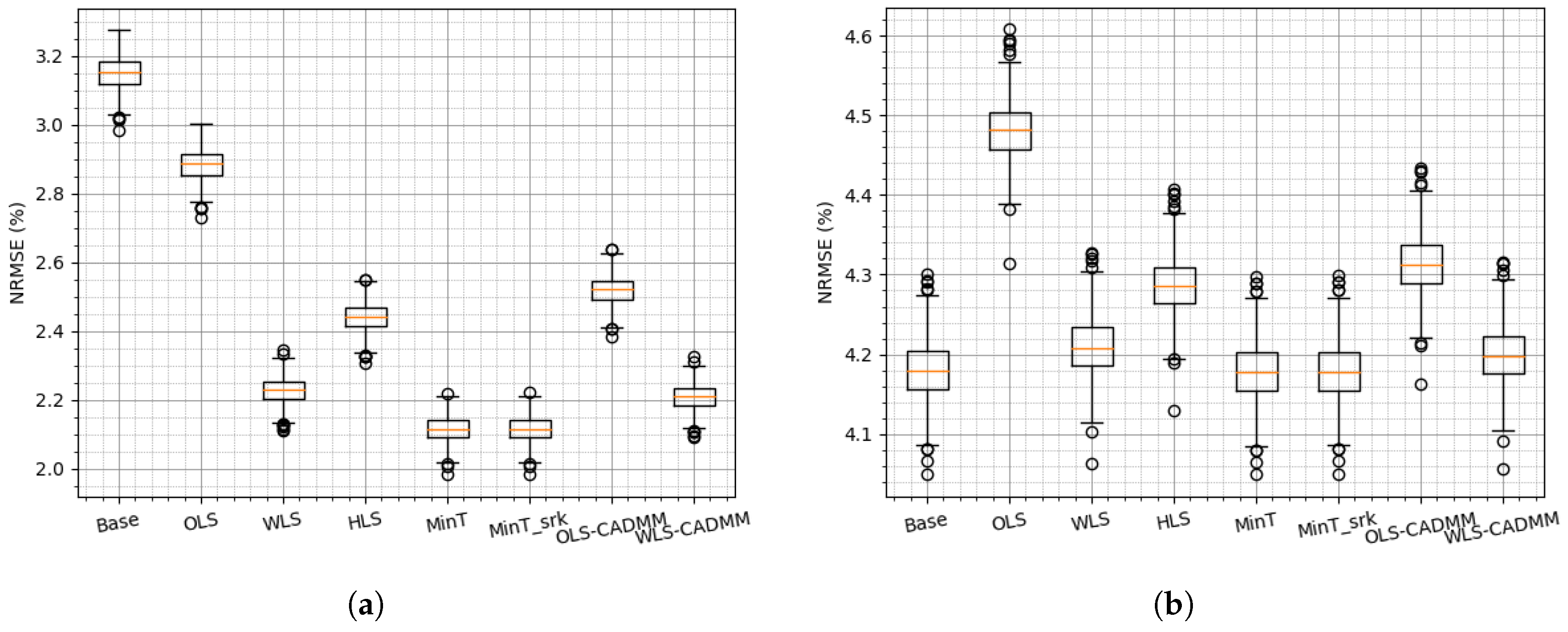
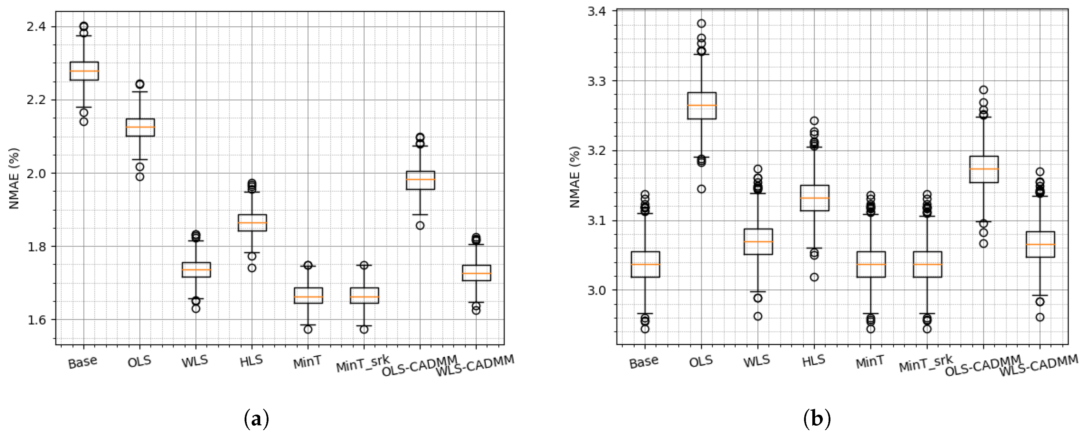
To evaluate the performance of reconciliation methods, the simulation is conducted 800 times with the same parameter configuration to examine the sensitivity and robustness of different reconciliation methods. The boxplots of NRMSEs and NMAEs are drawn to show the probabilistic property among 800 times simulations. As the simulation is carried on a two-level hierarchy of one aggregated node and five distributed nodes, the effects of the reconciliation methods are examined on both levels and the results are presented in Figure 3 and Figure 4. Overall, it can be noted that MinT and MinT_srk provide the best results among all those reconciliation methods, which is consistent with the conclusion drawn in [7,8]. From the results of the aggregated node shown in Figure 3a and Figure 4a, it can be found that any reconciliation method exerts dramatic positive effects on the base forecasts of the aggregation. On the other hand, not all of the reconciliation methods help to improve the base forecast of bottom node as presented in Figure 3b and Figure 4b. It is implied that on-site information can contribute to accurate base forecasts for the distributed farm, while the locally available information of the aggregation is not enough to lead to accurate base forecasts for the aggregation.

It can be further noted that OLS reconciliation is the worst one compared with other reconciliation methods, and HLS reconciliation method is better than OLS and worse than the others. This could be explained by the fact that both OLS and HLS methods are applied using constant covariance assumption without any further information from datasets. The others take into account the datasets and update the covariance matrix online. Among WLS, MinT and MinT_srk reconciliation methods, WLS assumes that all the distributed nodes are individually independent, and updates the covariance matrix in a diagonal form. On the contrary, the latter two update covariance matrix in full form and perform slightly better than WLS, ensuing more computation cost and data transmission cost adversely. This motivates us to reconcile the base forecasts in WLS frame or GTOP frame to reduce cost in a distributed way and to improve the performance by adding more constraints $\mathcal{B}$. The results of (WLS- or OLS-) CADMM of constrained GTOP are presented in Figure 3 and Figure 4 and they are slightly better than the centralized methods (WLS or OLS) due to the extra constraint $\mathcal{B}$.

In summary, MinT and MinT_srk are slightly better than other methods, whereas they cannot be readily distributed. On the contrary, WLS (OLS) and CADMM, acting as centralized and distributed constrained GTOP, provide similar results on the simulated datasets.

4.3. Reconciliation on the NREL Dataset

NREL dataset comes from the Eastern Wind Integration dataset, provided by NREL and freely available online [29,30]. In the NREL dataset, forecast wind speeds and the simulated wind farm power outputs are available. Despite this case study includes the simulated data, we have it for comparison purposes, as it has already been used to test reconciliation strategies in [7]. To be coherent, the NREL data corresponding to all six wind farms located in Kentucky in America are selected, as the geographical and data scales are comparable to the island Sardinia. Since the covariance matrix involved in the reconciliation methods is updated with dataset along timeline in (10), the datasets are divided in temporal order. The time duration of all the datasets is one year (8784 timestamps), among which the first 80% is used as training (64%) and validation dataset (16%), and the rest 20% as test datasets.

The performance of the reconciliation methods are presented in terms of NRMSE and NMAE in

Table 4. NRMSE (%) of National Renewable Energy Labaratory (NREL) dataset.

	Node 1	Node 2	Node 3	Node 4	Node 5	Node 6	Bottom Level	Node AGG
Base	7.76	6.62	6.96	6.88	6.75	7.44	7.07	10.90
OLS	16.69	17.68	17.35	8.88	9.92	8.90	13.24	9.95
WLS	7.73	6.63	6.96	7.23	6.92	8.18	7.28	6.28
OLS-CADMM	8.34	7.25	7.56	7.74	7.67	8.43	7.83	6.91
WLS-CADMM	7.73	6.63	6.96	7.19	6.92	8.02	7.24	6.23

and

Table 5. NMAE (%) of NREL dataset.

	Node 1	Node 2	Node 3	Node 4	Node 5	Node 6	Bottom Level	Node AGG
Base	5.34	4.62	4.82	4.90	4.79	5.18	4.94	6.65
OLS	9.73	9.48	9.53	6.11	6.55	6.06	7.91	6.25
WLS	5.34	4.64	4.83	5.18	4.91	5.68	5.09	4.49
OLS-CADMM	6.16	5.36	5.55	5.54	5.51	5.83	5.66	4.96
WLS-CADMM	5.34	4.64	4.83	5.14	4.91	5.57	5.07	4.45

. It can be found that the results on NREL dataset are consistent with the counterparts on the simulated dataset.

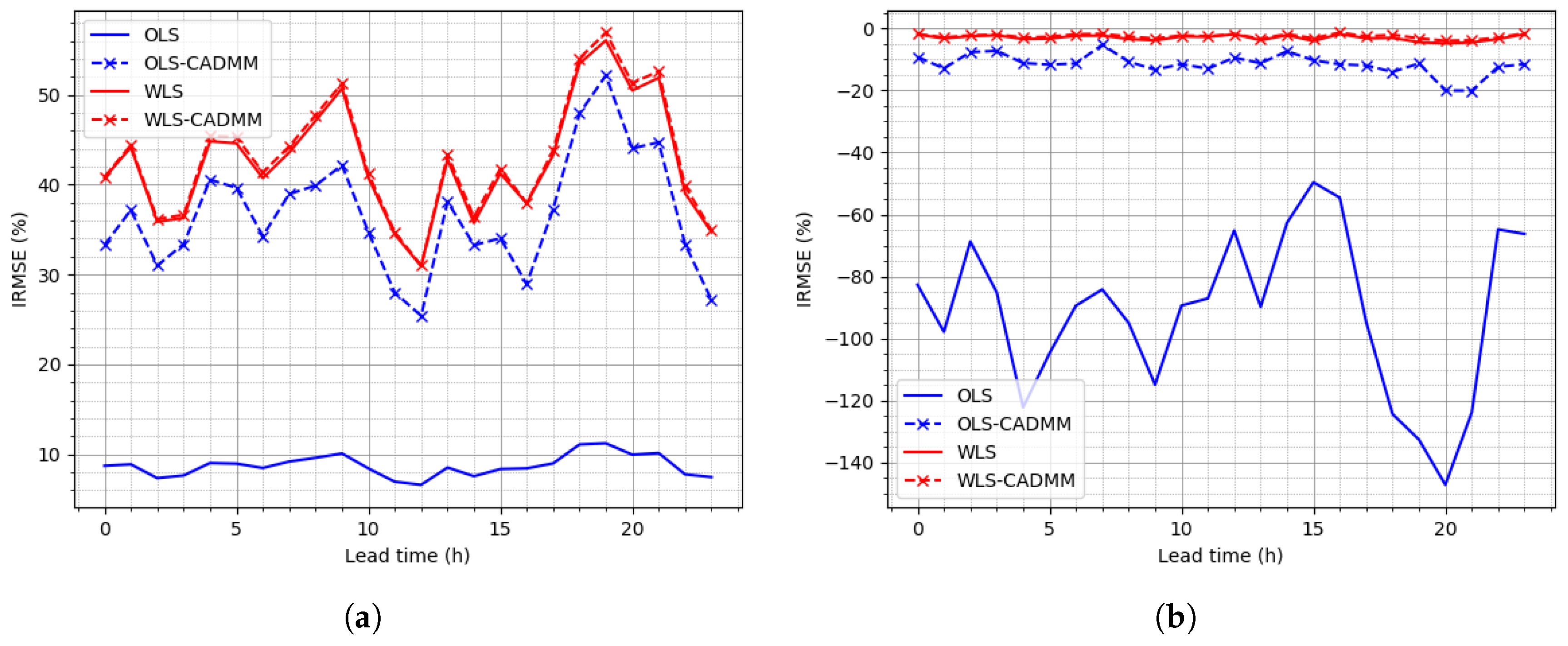
To clearly display the results obtained in centralized and distributed manners of GTOP under different frameworks (OLS or WLS), the overall scores of SNMSE in

Table 6. Summation of NMSE (SNMSE) (%) of NREL dataset.

Base	OLS	WLS	OLS-CADMM	WLS-CADMM
4.34	13.13	3.68	4.29	3.63

show that WLS-CADMM provides the best performance on average. In addition, the curves of IRMSE versus lead time at the top and bottom level presented in Figure 5 display that WLS outperforms OLS on the whole. WLS-CADMM offers a slight advantage over WLS while OLS-CADMM achieves great improvement due to the extra constraint $\mathcal{B}$. As the dataset of NREL is partly simulated, IRMSE remains at the same level along lead time.

4.4. Reconciliation on the Sardinia Dataset

The Sardinia Dataset includes four wind farms located on the island of Sardinia in Italy. Both forecast wind speeds and actual wind farm power production are available. Since the wind power in the NREL dataset is modeled, all the data are already well pre-processed. However, in the Sardinia dataset, the wind power outputs are primary data and contain abnormal data. Part of data cleaning techniques in [31] such as missing data processing and physical range check are adopted to remove outliers. Since the covariance matrix involved in the reconciliation methods is updated with dataset along timeline in (10), the datasets are divided in temporal order. The time duration of all the datasets is one year (8784 timestamps), among which the first 80% is used as training (64%) and validation dataset (16%), and the rest (20%) as test datasets.

Since the power outputs in the Sardinia dataset are measured, not modeled or simulated as the other two datasets, the performance of the reconciliation methods are largely different and are presented in terms of NRMSE and NMAE in

Table 7. NRMSE (%) of Sardinia dataset.

	Node 1	Node 2	Node 3	Node 4	Bottom Level	Node AGG
Base	11.68	9.15	12.29	12.40	11.38	7.56
OLS	11.54	8.93	11.96	12.12	11.14	7.61
WLS	11.55	9.05	12.21	12.29	11.28	7.76
OLS-CADMM	11.54	8.93	11.96	12.12	11.14	7.61
WLS-CADMM	11.60	9.07	12.15	12.28	11.27	7.76

and

Table 8. NMAE (%) of Sardinia dataset.

	Node 1	Node 2	Node 3	Node 4	Bottom Level	Node AGG
Base	7.11	4.90	7.69	7.71	6.85	4.94
OLS	7.09	4.85	7.67	7.65	6.81	4.95
WLS	7.09	4.86	7.67	7.68	6.82	4.98
OLS-CADMM	7.09	4.85	7.67	7.65	6.81	4.95
WLS-CADMM	7.14	5.12	8.02	7.90	7.04	5.08

. On the whole, there are no significant differences among the results of different methods.

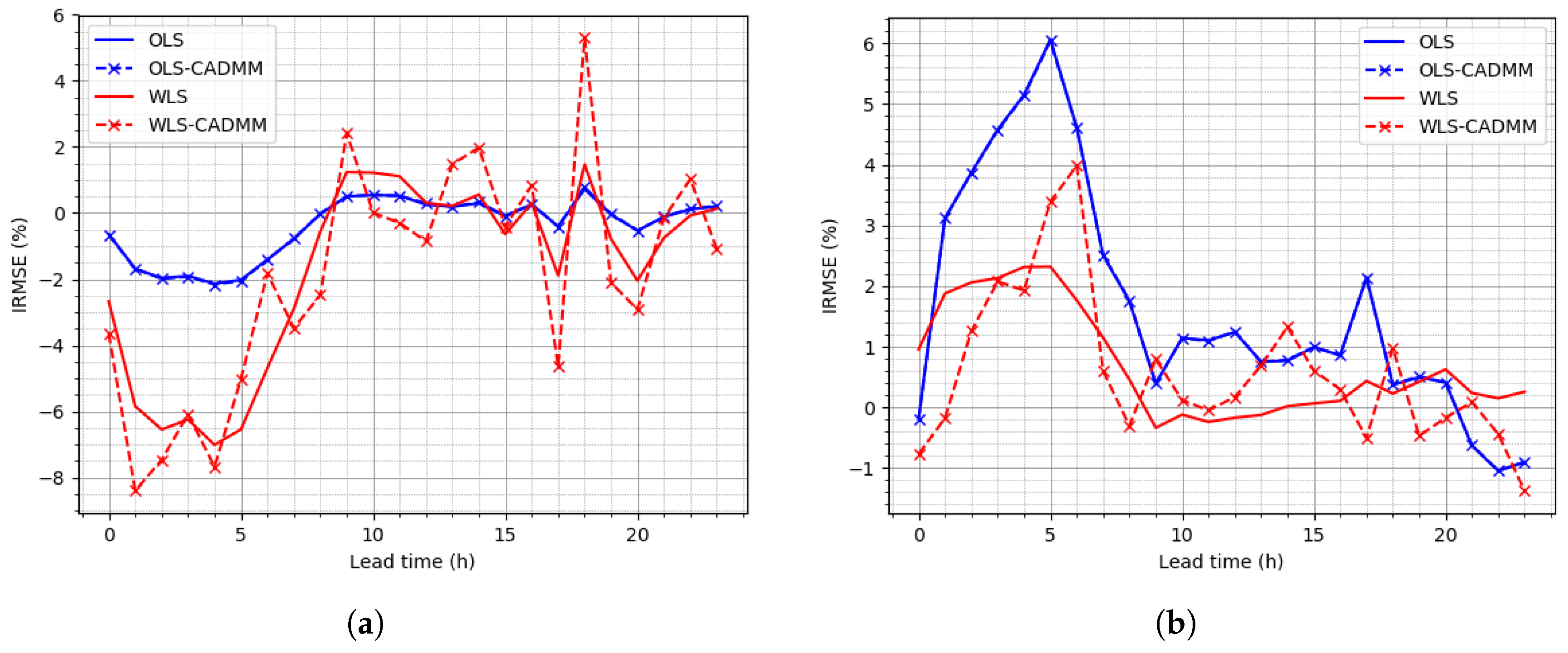
To focus on the performances of the centralized and distributed methods, the overall scores of SNMSE presented in

Table 9. SNMSE (%) of Sardinia dataset.

Base	OLS	WLS	OLS-CADMM	WLS-CADMM
5.82	5.61	5.75	5.61	5.75

and the results of IRMSE presented in Figure 6 indicate that OLS performs slightly better than WLS on average, which is opposite to their performances on the NREL dataset. CADMMs does not yield any dramatic improvement over OLS or WLS reconciliation with the extra constraint $\mathcal{B}$. It is also mentioned in [11] that the constraint does not have a large effect. Besides, it can be noted clearly in Figure 6b that IRMSE drops after the first several lead timestamps in that the base forecasts of the latter timestamps are poorly made because of inaccuracy of wind speed forecasts.

Overall, based on our simulated datasets and previous results in the literature, it may be that MinT and MinT_srk reconciliation methods achieve the most robust performance on the average. However, it requires the private data exchange among different data providers. On the contrary, the WLS or OLS reconciliation problem in GTOP framework can be solved in a distributed manner by ADMM to protect data privacy. Though the datasets involved in the case studies above are not sustantial enough, the consistency of the results in the simulated and NREL datasets indicates that the WLS reconciliation can be a good option to make reconciliation on the dataset of high quality or having high correlation determined by geographical closeness, and can be solved in a distributed way. On the contrary, the last case study on Sardinia dataset implies that low-quality dataset, contributing to a loose correlation, makes the OLS reconciliation efficient and effective and can further be solved with ADMM to preserve data privacy.

5. Conclusions and Perspectives

In this paper, state-of-the-art reconciliation methods are applied on day-ahead short-term wind power forecasts where hourly wind power base forecasts are made by using available wind speed information provided by NWP. A geographical hierarchy of wind power time series reconciliation problem is formed by taking into account differently located wind farms in the same region. A constrained GTOP reconciliation problem is solved in a distributed way using ADMM algorithm, in order to protect data privacy among different nodes (wind farms) in a hierarchy. Three case studies are carried out to examine the performance of those reconciliation methods: The first simulated dataset is generated to show a general performance, the latter two datasets are applied to evaluate the performances in specific scenarios. The results show that MinT provides the best performance by considering the correlation among different nodes in a centralized way. It could be considered to group the correlated nodes as one node if sharing data is allowed among certain nodes, and then the reconciliation can be solved in a distributed manner together with other loosely correlated nodes in the framework of (WLS-) GTOP. As we proposed to use ADMM to solve this problem in a distributed manner, other types of distributed optimization methods could also be envisaged e.g., dual decomposition.

References

- Fliedner, G. Hierarchical forecasting: Issues and use guidelines. Ind. Manag. Data Syst. 2001, 101, 5–12. [Google Scholar] [CrossRef]
- Christoph, W. Essays in Hierarchical Time Series Forecasting and Forecast Combination. Ph.D. Thesis, University of Cambridge, Cambridge, UK, 2018. [Google Scholar]
- Lobo, M.G.; Sanchez, I. Regional wind power forecasting based on smoothing techniques, with application to the spanish peninsular system. IEEE Trans. Power Syst. 2012, 27, 1990–1997. [Google Scholar] [CrossRef]
- Fabbri, A.; Roman, T.G.S.; Abbad, J.R.; Quezada, V.H.M. Assessment of the cost associated with wind generation prediction errors in a liberalized electricity market. IEEE Trans. Power Syst. 2005, 20, 1440–1446. [Google Scholar] [CrossRef]
- Lu, Z.; Ye, X.; Qiao, Y.; Min, Y. Initial exploration of wind farm cluster hierarchical coordinated dispatch based on virtual power generator concept. CSEE J. Power Energy Syst. 2015, 1, 62–67. [Google Scholar] [CrossRef]
- Meng, K.; Zhang, W.; Li, Y.; Dong, Z.Y.; Xu, Z.; Wong, K.P.; Zheng, Y. Hierarchical SCOPF considering wind energy integration through multiterminal VSC-HVDC grids. IEEE Trans. Power Syst. 2017, 32, 4211–4221. [Google Scholar] [CrossRef]
- Zhang, Y.; Dong, J. Least Squares-based optimal reconciliation method for hierarchical forecasts of wind power generation. IEEE Trans. Power Syst. 2018, 1. [Google Scholar] [CrossRef]
- Yang, D.; Quan, H.; Disfani, V.R.; Liu, L. Reconciling solar forecasts: Geographical hierarchy. Sol. Energy 2017, 146, 276–286. [Google Scholar] [CrossRef]
- Hyndman, R.J.; Lee, A.J.; Wang, E. Fast computation of reconciled forecasts for hierarchical and grouped time series. Comput. Data Anal. 2016, 97, 16–32. [Google Scholar] [CrossRef]
- Athanasopoulos, G.; Hyndman, R.J.; Kourentzes, N.; Petropoulos, F. Forecasting with temporal hierarchies. Eur. J. Oper. Res. 2017, 262, 60–74. [Google Scholar] [CrossRef]
- van Erven, T.; Cugliari, J. Game-theoretically optimal reconciliation of contemporaneous hierarchical time series forecasts. In Modeling and Stochastic Learning for Forecasting in High Dimensions; Springer International Publishing: Cham, Switzerland, 2015; pp. 297–317. [Google Scholar]
- Lei, M.; Shiyan, L.; Chuanwen, J.; Hongling, L.; Yan, Z. A review on the forecasting of wind speed and generated power. Renew. Sustain. Energy Rev. 2009, 13, 915–920. [Google Scholar] [CrossRef]
- Giebel, G.; Brownsword, R.; Kariniotakis, G.; Denhard, M.; Draxl, C. The State-Of-The-Art in Short-Term Prediction of Wind Power: A Literature Overview, 2nd ed.; ANEMOS.plus: Paris, France, 2011. [Google Scholar] [CrossRef]
- Hong, T.; Pinson, P.; Fan, S. Global Energy Forecasting Competition 2012. Int. J. Forecast. 2014, 30, 357–363. [Google Scholar] [CrossRef]
- Siebert, N. Development of Methods for Regional Wind Power Forecasting. Ph.D. Thesis, École Nationale Supérieure des Mines de Paris, Paris, France, 2008. [Google Scholar]
- Yan, J.; Zhang, H.; Liu, Y.; Han, S.; Li, L.; Lu, Z. Forecasting the high penetration of wind power on multiple scales using multi-to-multi mapping. IEEE Trans. Power Syst. 2018, 33, 3276–3284. [Google Scholar] [CrossRef]
- Hyndman, R.; Athanasopoulos, G. Optimally reconciling forecasts in a hierarchy. Foresight 2014, 2014, 42–48. [Google Scholar]
- Hyndman, R.J.; Ahmed, R.A.; Athanasopoulos, G.; Shang, H.L. Optimal combination forecasts for hierarchical time series. Comput. Stat. Data Anal. 2011, 55, 2579–2589. [Google Scholar] [CrossRef]
- Wickramasuriya, S.L.; Athanasopoulos, G.; Hyndman, R.J. Optimal forecast reconciliation for hierarchical and grouped time series through trace minimization. J. Am. Stat. Assoc. 2018, 1–16. [Google Scholar] [CrossRef]
- Jooyoung, J.; Anastasios, P.; Fotios, P. Reconciliation of probabilistic forecasts with an application to wind power. arXiv, 2018; arXiv:1808.02635. [Google Scholar]
- Yang, D.; Quan, H.; Disfani, V.R.; Rodríguez-Gallegos, C.D. Reconciling solar forecasts: Temporal hierarchy. Sol. Energy 2017, 158, 332–346. [Google Scholar] [CrossRef]
- Campbell, S.; Meyer, C. Generalized Inverses of Linear Transformations; Society for Industrial and Applied Mathematics: Philadelphia, PA, USA, 2009. [Google Scholar] [CrossRef]
- Schäfer, J.; Strimmer, K. A shrinkage approach to large-scale covariance matrix estimation and implications for functional genomics. Stat. Appl. Genet. Mol. Biol. 2005, 4, 32. [Google Scholar] [CrossRef] [PubMed]
- Boyd, S.; Parikh, N.; Chu, E.; Peleato, B.; Eckstein, J. Distributed optimization and statistical learning via the Alternating Direction Method of Multipliers. Found. Trends Mach. Learn. 2011, 3, 1–122. [Google Scholar] [CrossRef]
- Goldstein, T.; O’Donoghue, B.; Setzer, S.; Baraniuk, R. Fast alternating direction optimization methods. SIAM J. Imaging Sci. 2014, 7, 1588–1623. [Google Scholar] [CrossRef]
- Harris, R.I.; Cook, N.J. The parent wind speed distribution: Why Weibull? J. Wind Eng. Ind. Aerodyn. 2014, 131, 72–87. [Google Scholar] [CrossRef]
- Lydia, M.; Kumar, S.S.; Selvakumar, A.I.; Kumar, G.E.P. A comprehensive review on wind turbine power curve modeling techniques. Renew. Sustain. Energy Rev. 2014, 30, 452–460. [Google Scholar] [CrossRef]
- Jowder, F.A. Wind power analysis and site matching of wind turbine generators in Kingdom of Bahrain. Appl. Energy 2009, 86, 538–545. [Google Scholar] [CrossRef]
- Draxl, C.; Clifton, A.; Hodge, B.M.; McCaa, J. The Wind Integration National Dataset (WIND) Toolkit. Appl. Energy 2015, 151, 355–366. [Google Scholar] [CrossRef]
- Pennock, K. Updated Eastern Interconnect Wind Power Output and Forecasts for ERGIS: July 2012. Available online: https://www.nrel.gov/docs/fy13osti/56616.pdf (accessed on 1 October 2012).
- Zheng, L.; Hu, W.; Min, Y. Raw wind data preprocessing: A data-mining approach. IEEE Trans. Sustain. Energy 2015, 6, 11–19. [Google Scholar] [CrossRef]
- Kramer, O.; Gieseke, F. Short-term wind energy forecasting using Support Vector Regression. In Proceedings of the 6th International Conference SOCO—2011 Soft Computing Models in Industrial and Environmental Applications, Salamanca, Spain, 6–8 April 2011; Corchado, E., Snášel, V., Sedano, J., Hassanien, A.E., Calvo, J.L., Ślȩzak, D., Eds.; Springer: Berlin/Heidelberg, Germany, 2011; pp. 271–280. [Google Scholar]
- Zeng, J.; Qiao, W. Support vector machine-based short-term wind power forecasting. In Proceedings of the 2011 IEEE/PES Power Systems Conference and Exposition, Phoenix, AZ, USA, 20–23 March 2011; pp. 1–8. [Google Scholar] [CrossRef]
Figure 1.
A two-level hierarchy for wind farms and related wind power forecasts in a portfolio or region of interest.
Figure 2.
Iterations of convergence versus of Alternating Direction Method of Multipliers (ADMM) and fast ADMM (regarding three datasets).
Figure 3.
boxplots of normalized root mean square errors (NRMSEs) on the simulated dataset: (a) NRMSE of Node “AGG”, (b) NRMSE at bottom level.
Figure 4.
boxplots of normalized mean absolute errors (NMAEs) on the simulated dataset: (a) NMAE of Node “AGG”, (b) NMAE at bottom level.
Figure 5.
Improvement of RMSEs (IRMSEs) on the NREL dataset: (a) IRMSE of Node “AGG”, (b) IRMSE at bottom level.
Figure 6.
IRMSEs on the Sardinia dataset: (a) IRMSE of Node “AGG”, (b) IRMSE at bottom level.