Multi-Output Conditional Inference Trees Applied to the Electricity Market: Variable Importance Analysis

Abstract

Predicting electricity prices and demand is a very important issue for the energy market industry. In order to improve the accuracy of any predictive model, a previous variable importance analysis is highly advised. In this paper, we propose an alternative framework to assess the variable importance in multivariate response scenarios based on the permutation importance technique, applying the Conditional inference trees algorithm and a $\varphi$-divergence measure. Our solution was tested in simulated examples as well as a real case, where we assessed and ranked the most relevant predictors for price and demand of electricity jointly in the Spanish market. The new method outperforms, in most cases, the outcomes achieved by the recently proposed techniques, Intervention prediction measure (IPM) and Sequential multi-response feature selection (SMuRFS). For the electricity market case, we identified the most relevant predictors among pollutant, renewable, calendar and lagged prices variables for the joint response of demand and price, showing also the effectiveness of the proposed multivariate response method when compared with the univariate response analysis.

1. Introduction

The implementation of electricity market reforms in the European Union and other western countries has strengthened the competitiveness in the market [1] requiring the participants (energy producers, traders, distribution companies, large consumers and governments) to operate efficiently in the market. This efficiency requires a highly accurate forecasting process for the demand and price of electricity [2]. For instance, a more accurate price forecast may allow power suppliers to make better investment decisions by adjusting their production of energy and hedging against volatility and hence, maximize their financial benefits. Energy buyers may be able to protect themselves against high prices. Large consumers could benefit by efficiently managing their energy consumption, which could potentially lower their costs. Governments, on the other hand, are interested in a more accurate forecasting process for price and demand in order to implement new environmental regulations and structure changes applied to the energy market, or integrating different electric markets [3], which could eventually have a positive impact on their economic growth [4].

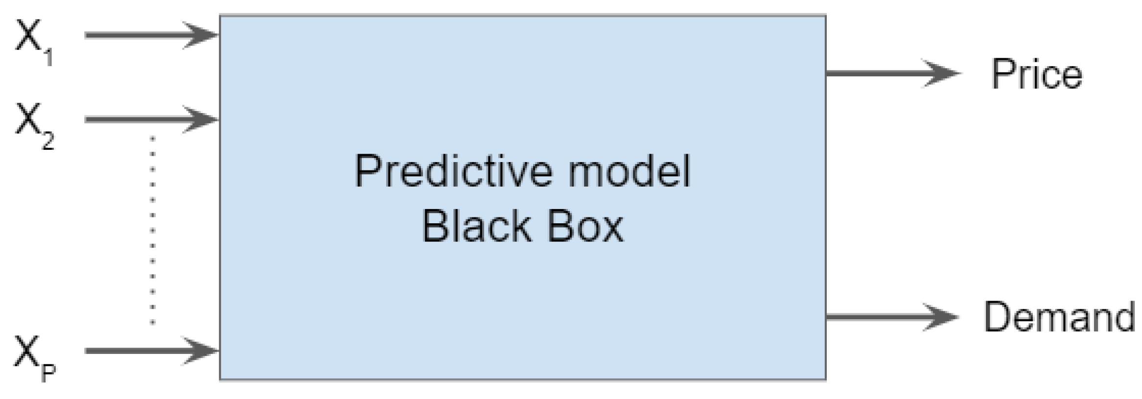
The current system established by governments aiming to introduce competitiveness among energy producers is based on economic pools [2], where producers bid on prices at which they are willing to generate the energy. In doing this, producers must take into account that this energy cannot be stored in large quantities, which creates the need to balance their production with the demand of electricity, in order to ensure that this demand is covered [5]. Hence, the market price is fixed every day for the following 24 h through the intersection between the supply of energy and the forecasted demand. This daily action system demonstrates the importance of predicting not only the price, but also the demand simultaneously so that the interdependencies between price and demand are taken into consideration [6]. Numerous forecasting techniques of price and demand of electricity have been used in recent years. Classical methods are based on statistical approaches such as, ARIMA [7,8], GARCH [9], or time-varying regression [10,11] (see [12] for recent advanced methods in electricity price forecasting). Machine learning techniques have also been proposed for this purpose [13,14,15,16,17]. However, the lack of interpretability due to the vast amount of data and the complex non-linear function (described as a black box in the literature) that maps the price and demand of electricity with the explanatory variables that drive the prediction of these outputs (Figure 1), makes a variable importance analysis a key pre-process step for any appropriate forecasting method. As a result of the dependencies between the demand and price, a multivariate response variable importance analysis is crucial in order to identify the predictors that have a high impact on the function responses. In this work, we propose a novel variable importance technique, the Euclidean probabilistic distance (EPD), based on a decision tree algorithm, the Conditional inference tree (CIT) algorithm, that allows us to gain insight into which variables are relevant for a forecasting model used to predict the demand and price of electricity simultaneously. The new proposed methodology will enable the electric energy participants to improve their decision-making mechanisms by identifying and understanding the explanatory variables, and their effect on the prediction of price and demand jointly, without having to repeatedly perform individual univariate analysis.

Literature: Variable Importance Analysis Electricity Market

Several papers regarding variable importance analysis (VIA) applied to the electricity market have been proposed. Nevertheless, only a few studied the multivariate response scenario. For instance, for the univariate response case, where the aim is the prediction of the price of electricity, ref. [18] proposed an algorithm to rank predictors involved in the Queensland (Australia) electricity market, based on the computation of information theory measures. Aimed at predicting the hourly electricity price in the Spanish and Australian markets, Amjady et al. presented a technique based on a two-stage feature selection process, consisting of a relief algorithm [19] and posteriori modified relief algorithm [20] which identified lagged prices $P_{t-1},P_{t-24}$, fuel costs and calendar indicators as the predictors with maximum relevancy to the electricity price, followed by a correlation analysis to eliminate redundant forecasters. Sood et al. [21] through correlation analysis identified relevant predictors (lagged prices $P_{t-1}$, load of previous days and weeks), capturing linear dependencies between predictors and the price of electricity involved in the Australian electricity market. Similarly, Keynia et al. [22] based their analysis of feature selection on a mutual information criterion, which provided a selection of relevant predictors for the price of electricity in the Spanish and Californian markets.

Lago et al. [3] applied ANOVA analysis (variance-based sensitivity analysis) that considers the effect of features (day-ahead prices, load and generation capacity and calendar variables) from connected European energy markets (Belgium and France). As a result, French prices and load account for nearly 50% of price prediction. A novel method, the Reference explanatory model for price estimations (REMPE), was developed by Monteiro et al. [23] to identify price variables $P_{t-1},P_{t-24}$, wind power, cogeneration and thermal variables as important to explain the prices a day ahead. Papers presented by [24,25] evaluated the influence of wind generation and day of the week on the Spanish electricity spot price.

The Shrinkage algorithm least absolute shrinkage and selection operator (LASSO) was used in [16,26]. While Ludwing et al. [26] compared LASSO and random forest algorithm to select the set of important weather variables involved in the forecasts of the German electricity spot prices, ref. [16] applied LASSO to extract the most influential variables in high dimensional settings (400 explanatory variables) in order to improve electricity forecasting models. Ziel et al. [17] compared univariate versus multivariate LASSO and identified among past electricity prices, calendar variables and periodic effects, the most significant predictors to be used in the predictions of the following 24 h electricity prices (multi-response analysis). The study revealed the importance of the 1 h lagged price, the day of the week and hour of the day as the variables with the highest impact on the multi-output predictive model. Close results were achieved by Misiorek et al. in [27].

The impact of fundamental variables was assessed in [28,29]. Keles et al. [29] applied a k-NN algorithm, while [28] investigated the impact of economic, technical (i.e., energy plant dynamics), strategic (i.e., market design) and other risk factors on intra-day electricity prices in the British market. Their analysis brought to light the importance of demand volatility (due to weather and consumption patterns), previous prices ($P_{t-1}$), diurnal and weekly effects for the price forecasting model. Results from [30] indicated that fundamental factors such as start-up cost, market states and tracking behavior explained approximately 75% of the intra-day price variance in the German electricity market. Carpio et al. [10] applied dynamic factor analysis to reduce the number of parameters involved in the prediction of multivariate time series hours electricity prices. Gonzalez et al. [31] evaluated the importance of fundamental and continuous variables applying tree-based algorithms for the Iberian electricity market.

Most recently, Febrero et al. [32], motivated by the problem of identifying the most relevant predictors for the demand and price of the Spanish electricity market and using a general additive regression model, proposed an algorithm based on the computation of distance correlations. With their variable selection solution, they were able to measure the level of redundancy among predictors of different scales. Different types of feature selection methods are evaluated and compared using different energy market data sets in [33,34,35].

Traditional univariate output techniques for variable importance analysis include the use of t-statistics, information theory measures or more sophisticated methods based on Bayesian approaches [36], support vector machine (SVM) [37], variance-based sensitivity analysis (SA) [38] (which consists of measuring how the variability of an input variable is propagated through the function model affecting the variance of the response variable) or the widely used parametric technique LASSO, a linear regression based method [39]. Although some of the mentioned techniques have been adapted to cope with multioutput variable problems ([40,41,42] for SA and Multi-task Lasso [43] for LASSO), these methods depend on the number of interaction terms included in the analysis, which makes the computations computationally expensive. On the other hand, multi-task lasso [43] only deals with linear correlations among predictors and performs poorly when coping with non-linear interactions. For these reasons, random forests [44,45], a non-parametric machine learning algorithm, has become a popular variable importance technique, thanks to its intrinsic feature selection capability, ability to cope with complex interactions, highly non-linear models, low-high dimension problems, different scale data set and easy scalability to multioutput scenarios [46,47,48,49,50].

To our knowledge, only the works described in [10,17] have analyzed the impact of explanatory variables when coping with multivariate response scenarios. In both cases, the multivariate response was the price of electricity at different hours. Consequently, no other papers are directly comparable to our work, where the aim is to analyze the influence of calendar effects, previous prices and energy production variables on the demand and price of electricity simultaneously. Our result would allow:

• Identify the relevant variables that affect the simultaneous prediction of the price and demand of any predictive model improving its accuracy (Feature selection pre-process).
• Analyze and measure (in terms of percentage of impact) the total effect of the predictors in a highly non-linear and multi-output scenario. The analysis provides useful information to the market participants that would allow them improve their market strategies.
• Multivariate analysis increases the speed of computation (processing time) and data storage efficiency.

The paper is structured as follows: Section 2 introduces the recent tree-based approaches related to the variable importance analysis (VIA) when coping with multi-output scenarios. Section 3.1 presents a sensitivity analysis of the hyper-parameters involved in the VIA. Section 3.2 describes the proposed methodology for VIA. In Section 4 we test our VIA methodology using numerical simulated examples and compare it to recently proposed solutions, IPM and SMuRFS. Section 5 is dedicated to estimating the most relevant predictors for price and demand jointly of the Spanish electricity market. We conclude our analysis in Section 6.

2. Tree-Based Methods for Multi-Output VIA

Among the recursive partitioning algorithms, the Conditional inference tree (CIT) algorithm has overcome the overfitting and bias towards predictors with many values when splitting [50]. The CIT algorithm measures at each node the association between input variables and response(s) using the permutation test theory [51], which allows for an unbiased selection of input variables for splitting.

According to our research, few tree-based methods have been proposed for variable importance analysis to deal with multi-output problems, mainly the Intervention prediction measure (IPM) [52] and the Sequential multi-response feature selection (SMuRFS algorithm) [53]. These techniques apply the frequency of appearance method [54] (i.e., relies on counting the number of times an input variable has been randomly selected at each inner node for splitting in the tree construction process) and hence do not take into account the possible connections among the responses in the analysis. The SMuRFS algorithm uses the CIT method to test for importance, filtering out insignificant features and giving a final list of survived input variables without ranking them. On the other hand, the IPM algorithm, also based on the CIT algorithm, derives the importance of variables from the structure of the tree, selecting variables as influential when they intervene in the prediction. (Comparison: tree-based variable importance techniques (VIT) for multi-output scenarios is found in

Table 1. Comparison: tree-based variable importance techniques (VIT) for multi-output scenarios.

VIT	Type	Advantages	Disadvantages
EPD	Based on permutation framework	Good performance non-linear scenarios. Less sensitive to $mtry$ selection	Only allows for continuous output variables.
IPM	Based on frequency of appearance framework	Allows for different scales of output variables	Underperforms in non-linear scenarios. Highly sensitive to $mtry$ hyperparameter selection.
SMuRFS	Based on frequency of appearance framework	Allows for different scales of output variables	Only provides list of survived covariates, not ranking values.

.)

We propose a new alternative for VIA, the Euclidean probabilistic distance (EPD) based on the Conditional inference tree algorithm (CIT), the permutation importance framework [45] (i.e., if an input variable $X_i$ has no influence in the output, then permuting its values will have no impact on the joint distribution $P(\overrightarrow{Y},\overrightarrow{X})$, which will lead to the same (when passing the out of bag observations through the tree) performance before and after permuting such a predictor) and a probabilistic measure. Our solution counts on a pre-process step to analyze the possible interrelations among the responses. A hyper-parameter sensitivity analysis is performed in order to provide some insight into what hyper-parameters (HPs) have more impact into the performance of the variable importance technique.

In order to assess our proposed technique for VIA, EPD, we use a parametric model based on sensitivity analysis as a standard reference to compare the non-parametric models EPD, SMuRFS and IPM. This standard reference model (referenced in this paper as PIT-SA) computes the sensitivity indices of the predictors (i.e., importance of each predictor) based on the Probability integral transformation [55]. PIT-SA considers, when computing the importance of input variables, the correlations among the responses and how those connections affect the ranking (Given $\overrightarrow{Y}=(Y_1,\dots ,Y_m)$ characterized by its CDF $V=F_Y(Y_1,\dots ,Y_m)$ the PIT of $\overrightarrow{Y}$ is defined as $K_V(v)=P(V<F_Y(Y_1,\dots ,Y_m))$. The sensitivity index corresponding to $X_i$ is: $S_i=\frac{1}{2}{E}_{X_i}(S(X_i))$, where, $E_{X_i}(S(X_i))={\int }_{\infty }^{\infty }{f}_{X_i}(x_i)[{\int }_0^1|K_V(v)-K_{V|x_i^{*}}(v)|]d{x}_i$. The larger $S_i$ the more important $X_i$ is for the multivariate output).

3. Proposal for Variable Importance Analysis

While dealing with multi-output problems, there are two ways to perform the variable importance analysis (VIA):

• Perform separate univariate VIA for each response, which ignores the correlations among responses. This alternative would work if the responses are highly correlated, however, the results would still be difficult to interpret.
• Perform a multivariate analysis either disregarding the connections among the responses (described methods: IPM and SMuRFS) or considering the possible connections (our proposed approach EPD).

3.1. Hyperparameter Sensitivity Analysis for Variable Importance Techniques

The accuracy of many variable importance techniques relies on how the hyperparameters (HPs) that govern the machine learning have been set. Therefore, as a first step, we propose a method to assess the relative importance of the HPs that control the precision of the used variable importance technique. In particular, we apply a method to study the importance of five HPs used to tune the CIT algorithm and also provide optimal values of these HPs. The optimal HPs values are later used to run the VIA to assess the relative importance of the predictors. The proposed method provides some insight into what HPs have relatively more impact on the performance of the VIA, which allows us to focus when tuning the algorithm on a small number of HPs when analyzing the problem.

The five HPs $\overrightarrow{\gamma }=[{\gamma }_1,{\gamma }_2,{\gamma }_3,{\gamma }_4,{\gamma }_5]$ used to calibrate the CIT algorithm are: ntree (number of trees in the forest), $mtry$ (number of input variables randomly selected to consider for splitting at each inner node), maxdepth (maximum depth of the tree), minsplit (minimum number of observations at each inner node in order to be considered for splitting), minbucket (minimum number of observations in a terminal node). Each HP can be configured using one of $K_i$ different values, which allows $D_{\gamma }=K_{1}x{K}_{2}x{k}_{3}x{k}_{4}x{K}_5$ combinations.

The analysis described in this Section 3.1 has been run for the univariate output scenario and p input variables. Although our main contribution in this paper is the Euclidean probabilistic distance algorithm for VIA in multi-output scenarios, the hyper-parameter sensitivity analysis for variable importance techniques, Section 3.1, provides information about how to tune the variable importance techniques used to perform the VIA. The procedure to study the relative importance of the HPs that control the performance of the described variable importance technique is:

• Build the hyperparameter matrix $H{P}_{matrix}(\overrightarrow{\gamma })$ (size $D_{\gamma }$x$|\gamma |$). Each row represents a different combination of HPs and each column a specific hyperparameter ${\gamma }_i$.
• Given a mathematical model $y=f(\overrightarrow{x}){|}_{\overrightarrow{x}=[x_1,\dots ,x_p]}$, compute the total Sobol sensitivity indices of the input variables ${VI|}_{Sobol}=[S_{T1},S_{T2},\dots ,S_{Tp}]$ (vector of total contributions, $S_{Ti}$, of the input variables to the variability of the response(s)). ${VI|}_{Sobol}$ is used as the standard reference.
• For each row of $H{P}_{matrix}(\overrightarrow{\gamma })$ (a different combination of hyper-parameters), compute ${VI|}_{CIT}(\overrightarrow{\gamma })$ = $[VI(X_1),\dots ,VI(X_p)]$ using the CIT algorithm (The trees are built using the data set $[y;\overrightarrow{x}]$, where $y=f(\overrightarrow{x})$. We use varimp() R function from “party” package to compute ${VI|}_{CIT}$). The step leads to a matrix (size $D_{\gamma }$xp) of variable importance (VI) values.
• Vectorize the ${VI|}_{CIT}(\overrightarrow{\gamma })$ matrix by computing row-wise the Euclidean distance (ED) between each row of ${VI|}_{CIT}(\overrightarrow{\gamma })$ and the standard reference ${VI|}_{Sobol}$. As result, we have a vector (Equation (1)) that describes the variability of ${VI|}_{CIT}(\overrightarrow{\gamma })$ with respect ${VI|}_{Sobol}$ in terms of the HPs $\overrightarrow{\gamma }$.

  $$V(\overrightarrow{\gamma })=ED(VI{|}_{Sobol}-row(VI{|}_{CIT}(\overrightarrow{\gamma })))$$

  (1)
• Given [$V(\overrightarrow{\gamma })$; $H{P}_{matrix}(\overrightarrow{\gamma })$], find the relationship $V(\overrightarrow{\gamma })=g_{ANN}(H{P}_{matrix}(\overrightarrow{\gamma }))$ (we use Artificial Neural Networks, ANN, to find the relationship).
• Given the ANN model, $V(\overrightarrow{\gamma })=g_{ANN}(H{P}_{matrix}(\overrightarrow{\gamma }))$, compute the main and interaction effects (sobol indices) of each HP involved in the performance of the variable importance technique and extract the optimal HPs values (values $\overrightarrow{\gamma }=[{\gamma }_1,{\gamma }_2,{\gamma }_3,{\gamma }_4,{\gamma }_5]$ that correspond to the minimum Euclidean distance between ${VI|}_{Sobol}$ and row(${VI|}_{CIT}$).

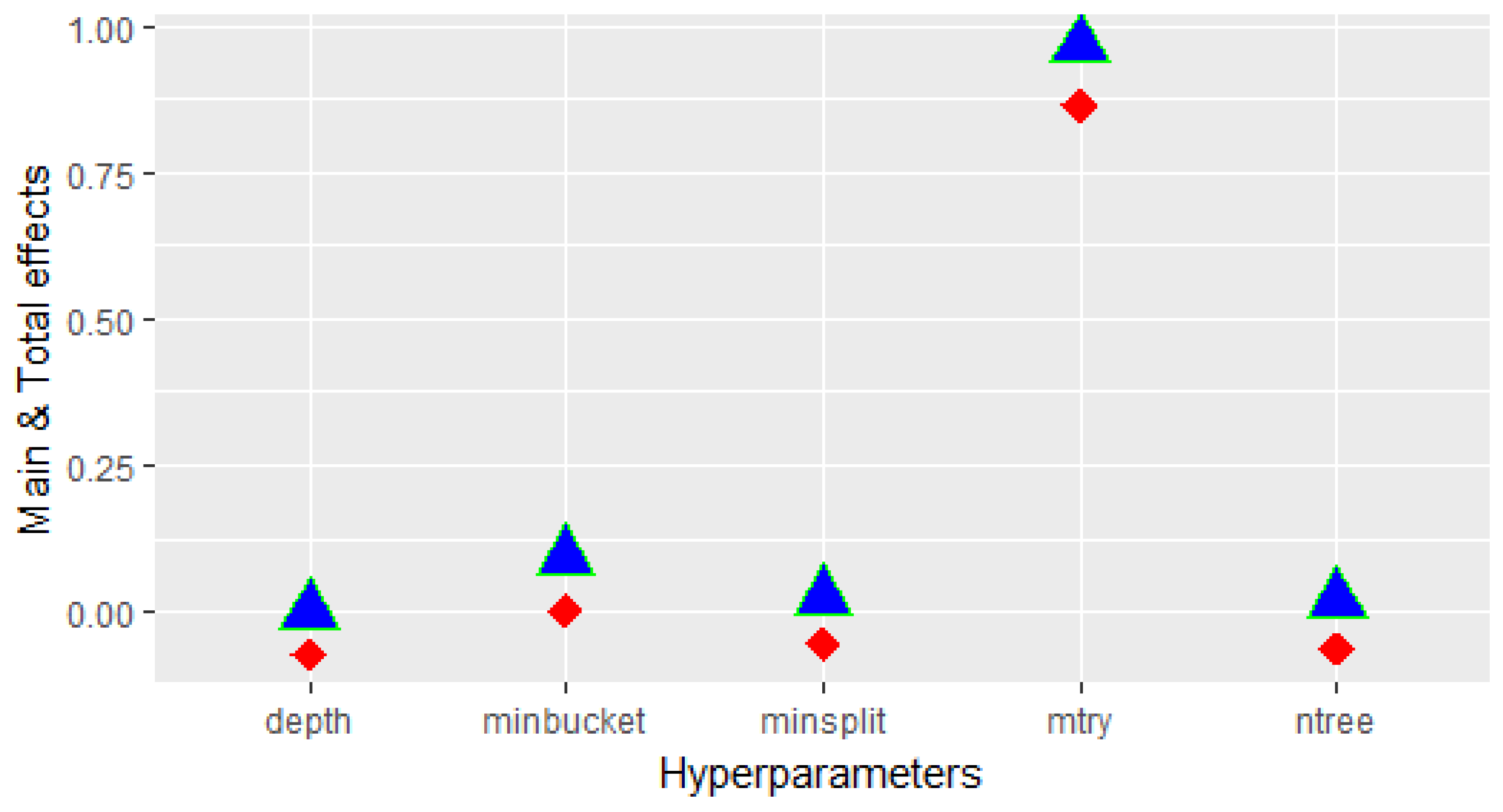
Figure 2 shows the main and total effects of each HP to the variability of the accuracy provided by the variable importance technique based on the CIT algorithm. As seen, the $mtry$ hyper-parameter has the highest impact on the precision of the variable importance technique.

3.2. VIA Based on EPD

The procedure EPD to assess the importance of input variables in a multi-output scenario consists of the following steps (see below VIA framework (Figure 3) and Algorithm 1):

• Given a data set $[\overrightarrow{Y};\overrightarrow{X}]$, described by m output and p input variables.
• (Pre-process step) Detect the linear dependencies among the output variables $\overrightarrow{Y}$ (see Khuri et al. [56] for detailed procedure). The goal is to drop responses that are linear functions of others.
  Given a matrix of responses (total m), $\overrightarrow{Y}=[Y_1,Y_2,\dots ,Y_m]$, we can perform the analysis of the possible dependencies by examining the matrix $D·D^{\prime }$, where D (Equation (2)) is defined as:

  $$D=Y^{\prime }·(\overrightarrow{e_N}-\frac{\overrightarrow{e_N}-\overrightarrow{e_N^T}}{N})$$

  (2)

  where, N is the number of observations and $\overrightarrow{e_N}$ a vector of ones of order (Nx1). We have “m linearly independent relationships exist among the responses if and only if $D·D^{\prime }$ has zero (or significantly small) eigenvalue $\lambda$ of multiplicity m”. Find m linearly independent eigenvectors $V=[\overrightarrow{V_1}:\overrightarrow{V_2}:\dots :\overrightarrow{V{\eta }_m}]$ corresponding to a zero eigenvalue (or small values) (then, $D^{\prime }·V=Z$, where Z is a matrix Nxm of very small elements). Decompose $V=[V_1^{\prime },V_2^{\prime }]$, where $V_1^{\prime }$ is a $m\times m$ matrix and the associated decomposition $D=[D_1^{\prime },D_2^{\prime }]$ where $D_1^{\prime }=-D_1^{\prime }·V_2·V_1^{-1}+E·V_1^{-1}$. Drop the responses that correspond to the columns of $D_1^{\prime }$ that match the rows of the optimal submatrix $V_1^{-1}$, which is the matrix that corresponds to the smallest value $||V_1^{-1}||$ (Euclidean distance).
• (Pre-process step) Standardize the variables.
• Extract the out of bag (OOB) observations $[{\overrightarrow{Y}}_{OOB};{\overrightarrow{X}}_{OOB}]$ from data set (save the observation matrix, abbreviated as $Y_{OOB}$).
• Built each tree using the CIT algorithm with the in of bag (IOB) observations $[{\overrightarrow{Y}}_{IOB};{\overrightarrow{X}}_{IOB}]$.
• Before permuting (BP) $X_i$ (input variable under analysis, i.e., a specific column in ${\overrightarrow{X}}_{OOB}$), we propagate the OOB observations ${\overrightarrow{X}}_{OOB}$ through each tree, resulting in the prediction matrix, $Y_{PRE{D}_{BP}}=CIT({\overrightarrow{X}}_{OOB})$ (prediction of each OOB observation of each response).
• Compute the Euclidean distance row-wise between the observation matrix $Y_{OOB}$ (Step 4) and the prediction matrix $Y_{PRE{D}_{BP}}$ (Step 6). The result is a vector of Euclidean distances $d^{BP}$ (vectorization) of size the number of OOB observations.
• Permute (AP) $X_i$ in ${\overrightarrow{X}}_{OOB}$ and use this permuted OOB observations ${\overrightarrow{X}}_{OO{B}_{X_i}}$ to compute the new prediction matrix $Y_{PRE{D}_{AP}}=CIT({\overrightarrow{X}}_{OO{B}_{X_i}})$.
• Compute the Euclidean distance row-wise (vector $d^{AP}$) between the observation matrix $Y_{OOB}$ (Step 4) and the new prediction matrix $Y_{PRE{D}_{AP}}$ (step 8). If the predictor $X_i$ is not relevant, then ${\mu }_{AP}\approx {\mu }_{BP}$ and ${\sigma }_{AP}\approx {\sigma }_{BP}$ (Note ${\mu }_{AP}=mean(d^{AP})$ and ${\sigma }_{AP}=std(d^{AP})$). Find the type of distributions (Kolmogorov Smirnov Test) followed by $d^{AP}$ and $d^{BP}$ to know what type of probability distance we should compute.
• Compute the probability distance (PD) (Jensen–Shannon distance (JSD) or ${\chi }^2$-distance) between the Euclidean probability distributions, $d^{AP}$ and $d^{BP}$ (a large value of JSD or ${\chi }^2$-distance shows that the empirical distributions belong to different sources, hence permuting the predictor under analysis $X_i$ has led to a significant deviation on the joint distribution, reflecting the importance of that predictor). Record the result of this computation.
  • if$d^{BP}$ and $d^{AP}$ are normally distributed then
    • Compute Jensen–Shannon distance $JSD(d^{AP},d^{BP})$ (Equation (3))
      Given two probability distributions $P_1$ and $P_2$ and $M=\frac{1}{2}(P_1+P_2)$, mathematically JSD is defined as:

      $$JSD(P_1,P_2)=\sqrt{(H(M)-\frac{1}{2}H(P_1)-\frac{1}{2}H(P_2))},$$

      (3)

      where $H()$ is the Shannon Entropy.
  • else
    • Given two probability distributions, $d^{BP}$ and $d^{AP}$, characterized by their histograms, $P_1$ and $P_2$, the ${\chi }^2$-distance (Equation (4)) between them is defined as:

      $${\chi }^2(P_1,P_2)=\frac{1}{2}\sum _{i=1}^d\frac{{(P_{i1}-P_{i2})}^2}{(P_{i1}-P_{i2})}$$

      (4)

      where d is the number of bins in the histograms.
  • end if
• Repeat steps 4 to 10 $ntree$ times. Each time, save the result in a vector size $ntree$. This leads to a vector of importance corresponding to $X_i$ over all trees of the forest (denoted in Algorithm 1 by vector PD).
• Finally, the importance of $X_i$, $VIM(X_i)$, is the mean of the vector calculated in the previous (step 11).
• Repeat steps 5 to 12 for all input variables $X_i{|}_{i=1,\dots ,p}$. This leads to a vector of importance (vecimp in Algorithm 1) which represents the relative importance of each input variable.
• Through the Gram–Schmidt (GS) orthogonalization procedure [57] (Equation (5)) applied to the multi-output response (i.e., we transform $T_{GS}:R^M\to R^M$ the multivariate output $Y=[Y_1,Y_2,\dots ,Y_M]\in R^M$ into a new orthogonal and independent set of output variables $Y^{\perp }=[Y_1^{\perp },Y_2^{\perp },\dots ,Y_M^{\perp }]\in R^M$) we can repeat the VIA and work with orthogonal and independent responses. This would allow us to measure to what extent permuting $X_i$ contributes to the variability of the responses independently, leading to $VIM(X_i){|}_{GS}$. The GS procedure:

  $$\begin{array}{c}{Y}_1^{\perp }=Y_1\hfill \\ Y_i^{\perp }=Y_i-E[Y_i|Y_1^{\perp },\dots ,Y_{i-1}^{\perp }]\vee i=2,\dots ,M\hfill \end{array}$$

  (5)

Algorithm 1 Variable importance analysis (VIA) Euclidean probabilistic distance (EPD) algorithm.

1: Dataframe (Dataset)  2: Find dependencies, Standardize, Orthogonalization  3: $\mathbf{vecimp}=0$ (Vector holding the relative importance $VIM(Xi)$ of all predictors)  4: $d_t^{BP}$ (Distribution Euclidean distances tree t before permuting)  5: $d_t^{AP}$ (Distribution Euclidean distances tree t after permuting)  6: ntrees (Total number of trees in the forest)  7: $\mathbf{vecimp}=c()$  8: for$nvar$ in $col(1\mathrm{st}\mathrm{inputvar}):ncol(Dataframe)$ do  9:      $PD=c()$ 10:   for $tree$ in $1:ntrees$ do 11:     Compute the predictions using OOB and CIT predictor model BP 12:     Calculate $d_t^{BP}=ED(OB{S}_j^{BP},PRE{D}_j^{BP})$ 13:     Permute the $X_i$ on the OOB dataset 14:     Compute the predictions using permuted OOB dataset 15:     Calculate $d_t^{AP}=ED(OB{S}_j^{AP},PRE{D}_j^{AP})$ 16:     Compute $P{D}_t(d_t^{AP},d_t^{BP})$ 17:     Store $PD=c(PD,P{D}_t)$ 18:   end for 19:   $VIM(Xi)=mean(PD)$ 20:   $\mathbf{vecimp}=c(\mathbf{vecimp},VIM(Xi))$ 21: end for 22: Return $\mathbf{vecimp}$

4. Numerical Simulations

The tree-based algorithms EPD, IPM and SMuRFS are compared using linear and non-linear models (the “IPMRF” R Package for IPM and the R function SMuRFS() for SMuRFS are used). In order to assess and compare the non-parametric techniques, we use, as a standard reference (only when continuous variables are involved, Section 4.2), a parametric method [55] based on the computation of Probability integral transformation (PIT-SA) of the multivariate response Y. PIT-SA takes into account the correlations among the responses and how the connections affect the ranking of the input variables. SMuRFS algorithm only provides a list of significant covariates, not ranking values (All the simulations have been run using the R Software).

4.1. Simulated Example: Linear Model

The studied model is: (2 output and 7 input variables) [52].

This simulated example consists of a continuous bivariate output and a combination of continuous (normal $X2,X4,X5$ and $X6$ and uniform $X3$) and categorical input variables (binomial $X1$ and $X7$),

Table 2. Input variables for linear model.

Variables	X1	X2	X3	X4	X5	X6	X7
Distributions	B(1,0.6)	N(3,1)	U(4,6)	N(5,1)	X2 + N(0,0.15)	P(X2)	P(X1)

. Variables $X6$ and $X7$ are permutations of the variables $X2$ and $X1$ respectively. According to the definition of the output variables $Y1$ and $Y2$,

Table 3. Output variables for linear model.

Variables	$\mathit{Y}\mathbf{1}\mathbf{|}\mathit{X}\mathbf{1}\mathbf{=}\mathbf{0}$	$\mathit{Y}\mathbf{1}\mathbf{|}\mathit{X}\mathbf{1}\mathbf{=}\mathbf{1}$	$\mathit{Y}\mathbf{2}\mathbf{|}\mathit{X}\mathbf{1}\mathbf{=}\mathbf{0}$	$\mathit{Y}\mathbf{2}\mathbf{|}\mathit{X}\mathbf{1}\mathbf{=}\mathbf{1}$
Model	$2+2·X2·N(0,0.1)$	$3+4·X2·N(0,0.2)$	$2+3·X2·N(0,0.15)$	$3+5·X2·N(0,0.2)$

, only $X1$ and $X2$ are directly involved in the prediction. $X5$ is defined to be highly correlated to $X2$ ($X5$ is $X2$ plus noise). The rest of the input variables are added to the model as noise.

The simulations have been run for three different $mtry$ values, $mtry\subset (1,4,7)$, $ntree=100$ and $N=120$ observations.

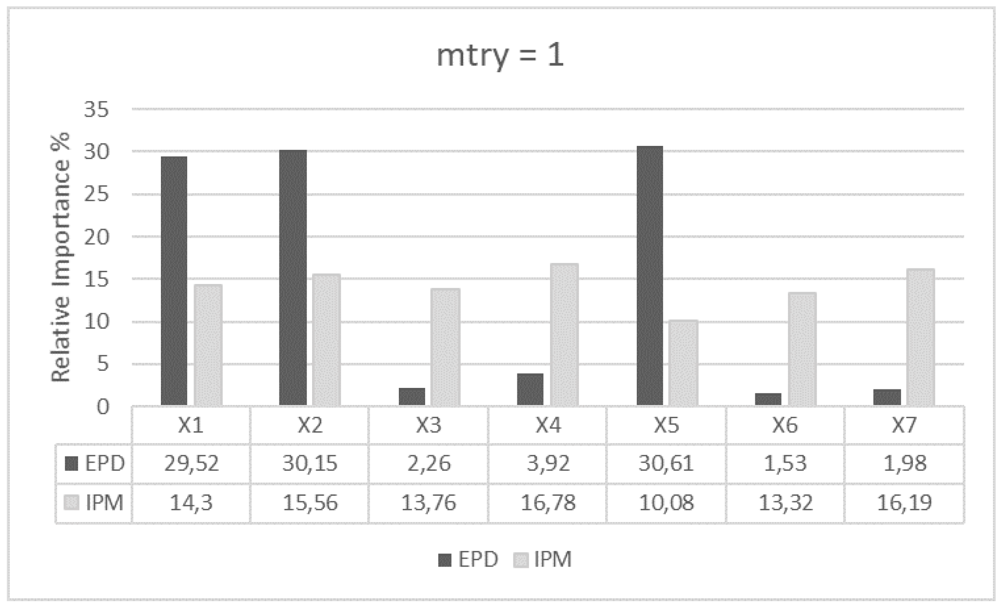
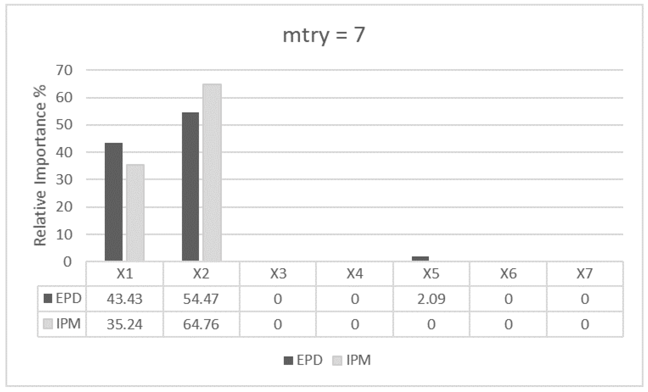
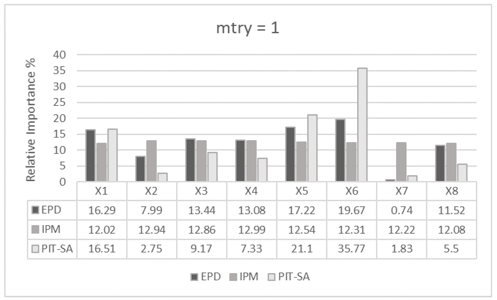
The following Figure 4, Figure 5 and Figure 6 show the relative importance of each input variable to the bivariate output for each VIA technique in terms of the hyper-parameter $mtry$ (as described in Section 3.1 variable importance techniques accuracy (VIT) is highly sensitive to the hyper-parameter $mtry$).

For $mtry=1$ (Figure 4), EPD distinguishes clearly between important ($X1$, $X2$ and $X5$) and non-important variables ($X3$, $X4$, $X6$ and $X7$). $X5$ also appears as significant in the ranking due to its correlation with $X2$. Using the same settings ($mtry=1$), IPM computes quite similar importance to all its input variables (IPM is quite flat while EPD shows a clear pattern). As we calibrate the value of $mtry$ from 1 to 4 and then 7, both algorithms, EPD and IPM, start providing values closer to the expected rankings, where only $X1$ and $X2$ are significant. Particularly, for $mtry=7$ (Figure 6), the algorithms rank $X2$ as the most important variable, followed by $X1$, having the remaining input variables a residual importance due to the randomness of the algorithms. Regardless of $mtry$, the list of survived input variables provided by SMuRFS is $X1$, $X2$ and $X5$. Comparing EPD and IPM, EPD ranks the predictors independently of the values of $mtry$, showing less sensitivity to the selection of $mtry$.

4.2. Simulated Example: Non-Linear Model

The studied model (Equation (6) and

Table 4. Variables for the non-linear model.

Variable	X1	X2	X3	X4	X5	X6	X7	X8
Distribution	Normal	Normal	Normal	Normal	Normal	Normal	Normal	Normal
Mean	$20,000$	12	$0.04$	$9.82$ × ${10}^{-4}$	$1.34$ × ${10}^7$	$3.35$ × ${10}^8$	2 × ${10}^{10}$	1 × ${10}^{11}$
Std	1400	$0.12$	$0.0048$	$5.892$ × ${10}^{-5}$	$2.412$ × ${10}^6$	$4.02$ × ${10}^7$	$0.12$ × ${10}^{10}$	$0.06$ × ${10}^{11}$

) is: (three output and eight input variables, $X_i$ are independent) [55].

$$\begin{array}{c}{Y}_1=0.03-\frac{1.905X_1{X}_2^2}{X_3{X}_7}-\frac{0.565X_1{X}_2^2}{X_4{X}_8}\hfill \\ Y_2=X_5{X}_3-1.185X_1{X}_2\hfill \\ Y_3=X_6{X}_4-0.75X_1{X}_2\hfill \end{array}$$

(6)

The simulations for the non-linear model have been run for $mtry\subset (1,4,8)$, $ntree=100$ and $N=$ 10,000 observations. $X2$ and $X7$ are set up to be non-influential input variables, while $X6$ and $X5$ the most influential.

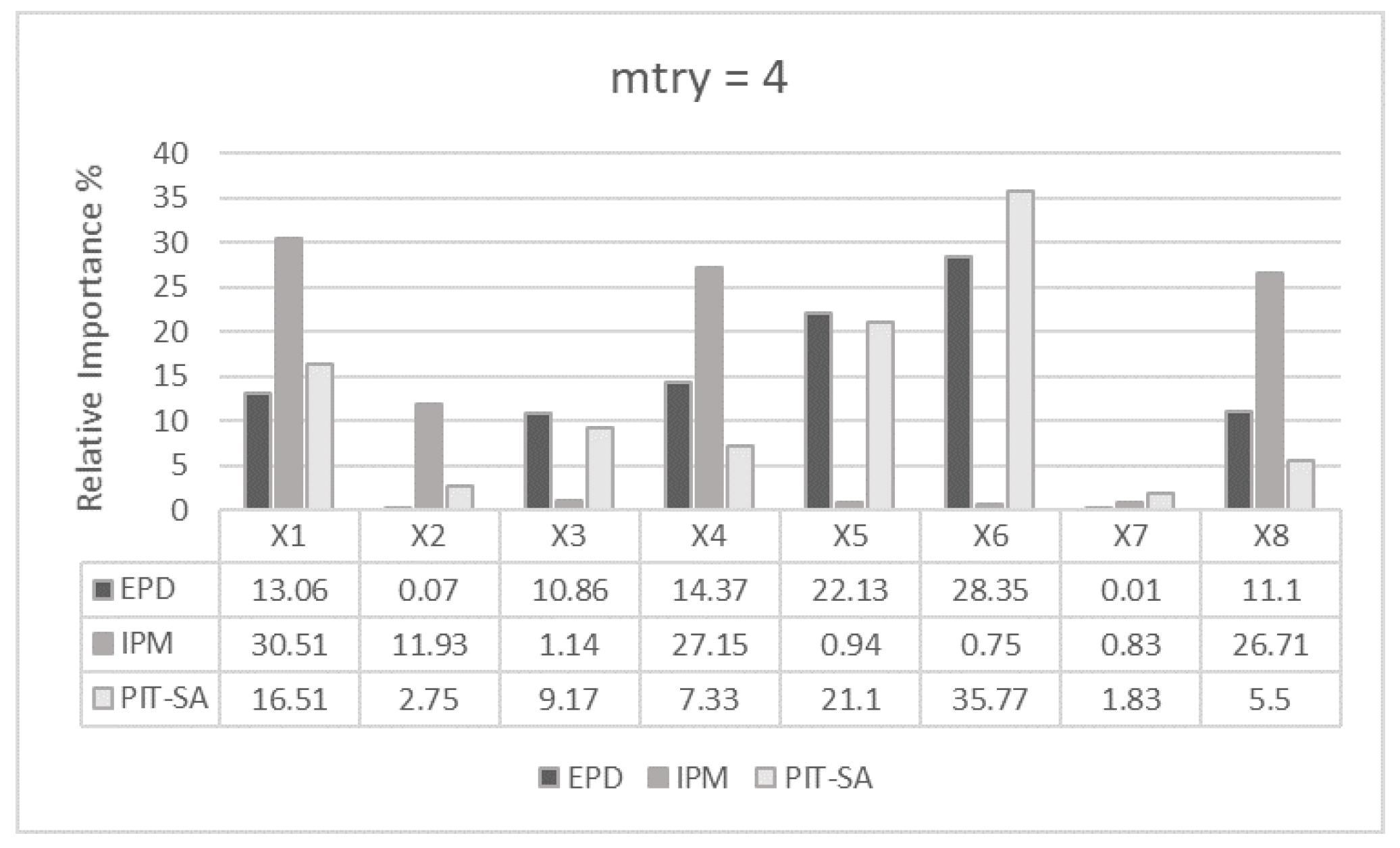
The following Figure 7, Figure 8 and Figure 9 show the relative importance of each input variable for each VIA technique in terms of the hyper-parameter $mtry$.

For $mtry=1$ (Figure 7), the ranking pattern provided by EPD is equal to the reference PIT-SA for all input variables. IPM, with $mtry=1$ (Figure 7), computes quite similar ranking values among all, showing almost no pattern (Figure 7). EPD and PIT-SA differences in ranking values start decreasing as we calibrate EPD algorithm by changing $mtry$, for instance, when $mtry=8$ (Figure 9), the difference in ranking is slight.

When comparing IPM ranking values to those of EPD and PIT-SA, differences in ranking are clear. For $mtry=4$, Figure 8, IPM considers $X3$, $X5$ and $X6$ having no effect on the trivariate output, ranking $X6$ as the least important when in contrast, EPD and PIT-SA have ranked it in the first position. The list of survived input variables (significant covariates) provided by SMuRFS is $X1$, $X3$, $X4$, $X5$, $X6$ and $X8$, which coincides with EPD and PIT-SA. These results lead us to understand that IPM underperforms when dealing with non-linear models.

5. Real Case: VIA Spanish Electricity Market

In any developed society, energy is a primary resource. Energy supply can be considered essential, ensuring wellness, stability and development.

Nowadays, in a global and interconnected society, energy supply can be considered a market where countries and public and private companies are capable of selling and buying energy according to their needs. The energy market involves five key elements: generation of electricity, transport, transmission, distribution and selling it to the consumer.

For energy generation, forecasting has become indispensable and to improve the accuracy of the forecast a previous variable importance analysis is crucial. The emergence of renewable energies (especially due to the policy applied in Spain since 2007) and their trend to become the main source of energy is an additional source of difficulty for the traditional energy producers to adjust their production. Traditional energy production includes thermal power plants and combined cycle, which are much more pollutant than renewable energies, such as wind farms or solar energy. In the Spanish electricity market, renewable energies are part of a special regime (REE: ‘Spanish transmission system operator’) and generally, facilities that produce renewable energy have a maximum installed capacity of 50 MW.

Pollutant ways of energy production are currently used for demand not covered by renewable sources. Due to the variability of renewable resources, a reliable energy production system should lean on thermal power plants and combined cycle, which can adjust their productions almost instantly when necessary.

Since energy cannot be stored in large quantities, energy producers have to schedule their production according to the variability of the rest of producers. This scheduling is a primary activity in order to ensure that production covers demand, allowing them to optimize their resources and become more competitive, and it is the main reason for the importance of forecasting the demand of electricity.

The Spanish energy market is specially complex since it adjusts energy prices using a ‘pool market’: prices are fixed at the figure at which the last producer used to cover demand offers energy. This means that, although some producers can offer their energy at price 0 Euros/MWh, they still get paid for this energy as long as price for the last energy used is not zero Euros/MWh, (OMIE: Spanish electricity price market operator). For this reason, renewable energy producers offer their energy at 0 Euros/MWh, and the rest of producers fix their prices according to demand. This explains that renewable energies are always chosen to cover demand. Therefore, price forecasting is also a main issue for energy producers and by thus for the energy market.

Considering the price and demand of Spanish electricity market as the response of our real model and using the new proposed method, EPD, we aim to measure the effect on the bivariate output of 15 input variables. We also compare the results provided by EPD to the IPM and SMuRFS techniques. The analysis will allow us to identify the non-important predictors that could undermine the accuracy of the forecasting model.

The predictor variables used to perform the analysis of variable importance are of two different types, nominal (type of day (ToD), day of the week (DoW), hour of the day (HoD), and month (M)) and continuous (lagged price one hour (P1h), lagged price two hours (P2h), lagged price 24 h (P24h), hydraulic energy production (H), nuclear energy production (N), coal energy production (C), fuel–gas energy production (FG), combined cycle energy production (CC), wind energy production (W), solar energy production (S), or other renewable energy production (OR)). The response variables are both continuous, demand and price of electricity. The data set used for this study includes hourly data from 01-05-2016 at 17:00 to 30-04-2018 at 23:00, extracted from Red Eléctrica de España (https://www.esios.ree.es/es) [58].

Table 5. Variables included in the data set.

Variable	Symbol	Type	Value
Demand	D-W (O)	Continuous	17,085–39,965 MWh
Price	Z-P (O)	Continuous	0–115 Euro/MWh
Type of day	TD (I)	Nominal	1 = W day, 2 = Weekend, 3 = Publ. Ho
Day of the week	DW (I)	Nominal	1–7 (days)
Hour of day	HD (I)	Ordinal	1–24 (hours)
Month	M (I)	Nominal	1–12 (Month)
Lagged price one hour	P1h (I)	Continuous	0–115 Euro/MWh
Lagged price two hours	P2h (I)	Continuous	0–115 Euro/MWh
Lagged price 24 h	P24h (I)	Continuous	0–115 Euro/MWh
Hydraulic energy prod.	H (I)	Continuous	420–12,050 MWh
Nuclear energy prod.	N (I)	Continuous	3500–7125 MWh
Solar Energy prod.	S (I)	Continuous	1–5980 MWh
Coal energy prod.	C (I)	Continuous	390–9660 MWh
Fuel-Gas energy prod.	FG (I)	Continuous	0–495 MWh
Combined cycle energy prod.	CC (I)	Continuous	330–12,320 MWh
Wind energy prod.	W (I)	Continuous	1500–15,000 MWh
Other renewable energy prod.	OR (I)	Continuous	3880–26,415 MWh

summarizes the input (I) and output (O) variables included in the variable importance analysis and their corresponding ranges.

5.1. Scenario 1: VIA Continuous Variables

In this first scenario, we analyze the effect of energy production (coal, combined cycle, wind, fuel–gas, hydraulic, nuclear, solar and other renewable) on the joint output variables, demand (W-D) and price (Z-P) of electricity. The correlation matrix (Figure 10) includes energy generation as well as lagged prices variables and the price and demand of electricity. The correlation between the Demand and Price is 0.56. The demand of electricity seems more correlated with all lagged prices and combined cycle, coal, solar and hydraulic energies (from higher to lower level of correlation). The combined cycle, coal and hydraulic correlation with the demand can be explained by the fact that these types of energy production can be more adjustable depending on the level of demand. On the other hand, the price is highly correlated with coal and combined cycle (energies expensive to produce) and less with Other Renewable, this last type of energy being the only renewable energy significantly correlated with price.

The simulation characteristics used in the CIT algorithm to test EPD and IPM methods were: $mtry=4$ and $ntree=100$.

The following Figure 11 shows the relative importance of each input variable to the bivariate response using the VIA techniques (the ranks for EPD and IPM are expressed in %), EPD, IPM and SMuRFS (SMuRFS only provides a list of survived covariates. In this scenario only FG is excluded (Non important covariate)).

Both variable importance techniques, EPD and IPM, show the same pattern. For EPD, pollutant energies (Coal, Combined cycle and Hydraulic) rank in the first three positions, having a 63.63% impact on Demand and Price jointly, while clean energies (Solar, Wind and Other renewable) contribute with 31.26%. It is reasonable to have the Coal, Combined cycle and Hydraulic energies as the most importance variables for demand and price, primarily for two reasons: First, in order to cover the demand that renewable energies (less reliable) cannot cover, pollutant energies are used, as their production are more adjustable. However, these energies are also more expensive to produce. The contribution of nuclear energy can be considered as residual (5.08%). With the exception of N and FG energies, all the predictors appear to have an influence on the joint response and hence should be included in the forecasting process.

5.2. Scenario 2: VIA Nominal Variables

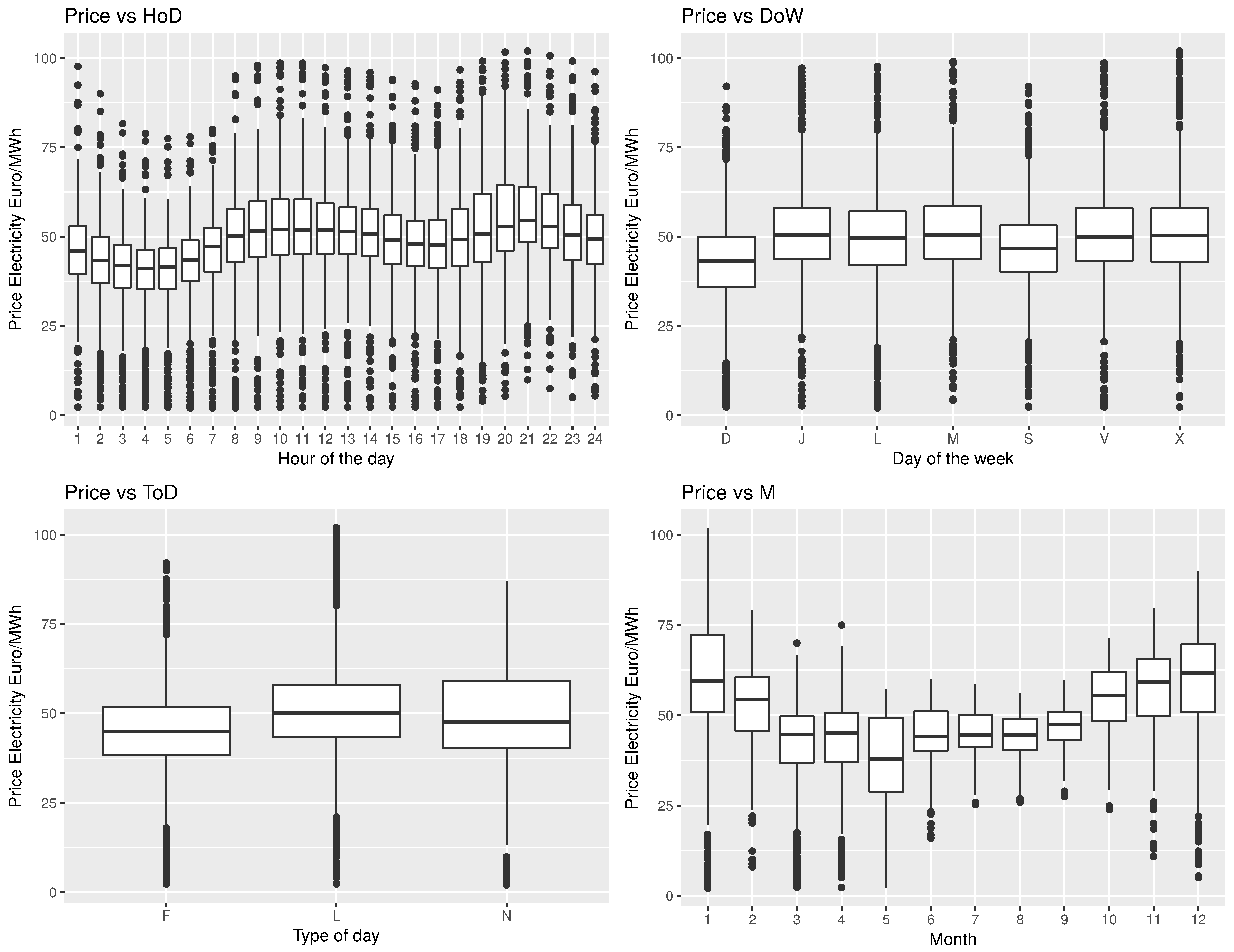
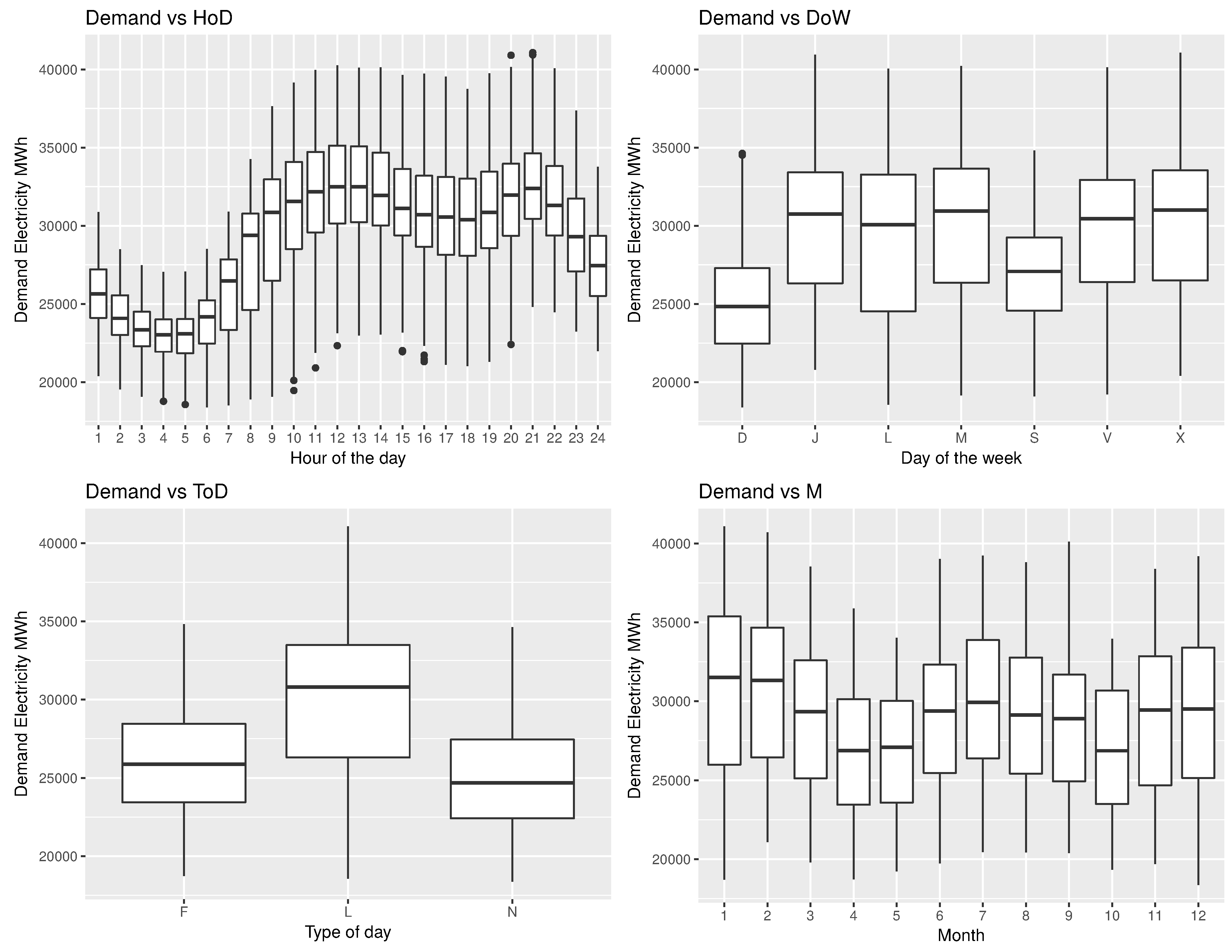
This scenario was set to study how different calendar variables (hours of the day, day of the week, type of day and month) impact the demand and price of electricity. Consistent with normal human and industrial/commercial behavior, there is a clear pattern seen by price and demand with respect to the hours of the days (Figure 12 and Figure 13), where at early hours along with non-working days (type of days, F: weekend and N: holiday) both the demand and price are low. Also as expected, on weekends the demand and price are lower than in business days, being higher in winter season (December, January and February) compared to spring.

The simulation characteristics used in the CIT algorithm to test EPD and IPM methods are: $mtry=2$ and $ntree=100$.

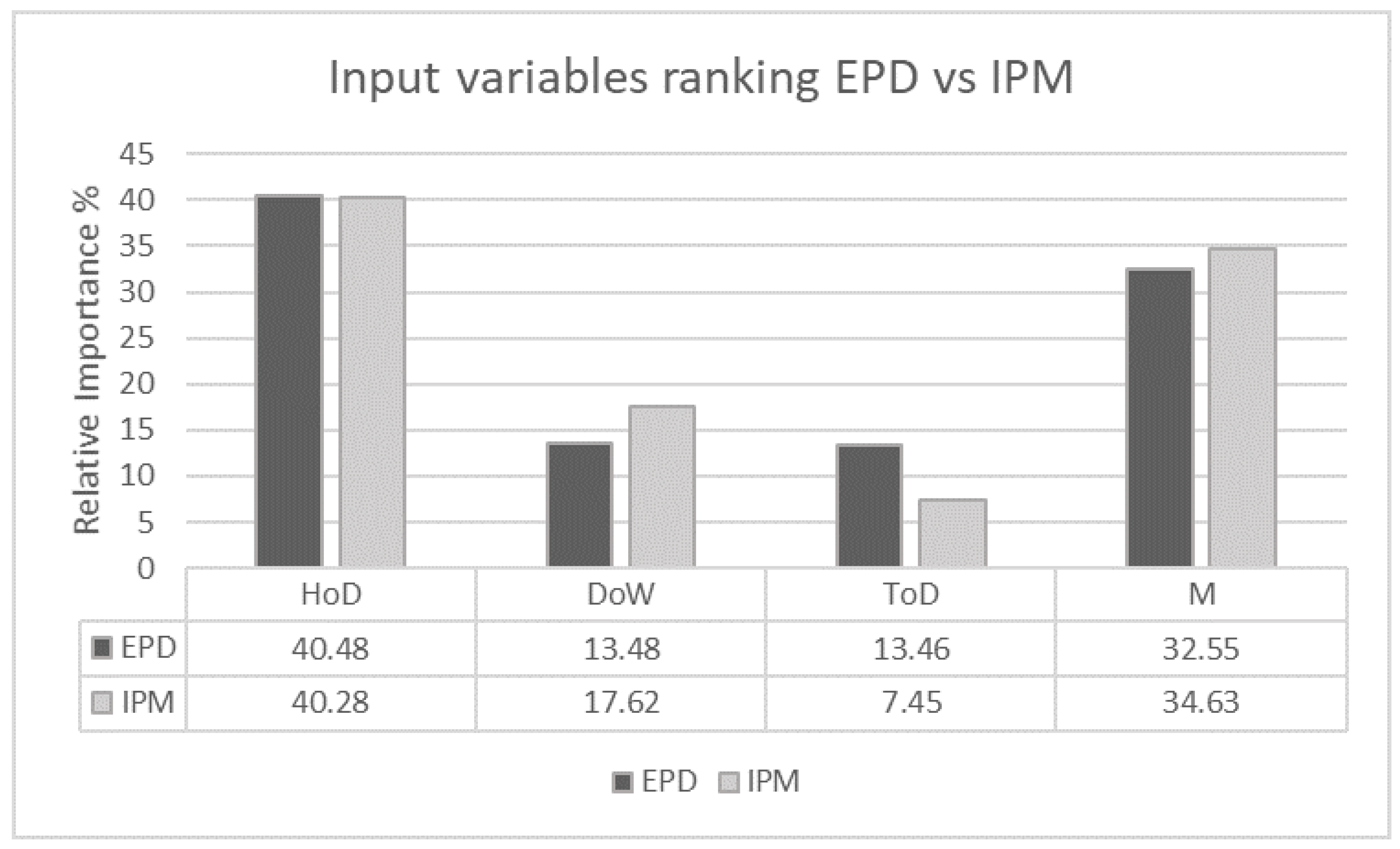
The following Figure 14 shows the relative importance of each input variable for the joint response demand and price using the VIA techniques, EPD and IPM.

The ranking provided by EPD and IPM are: HoD > M > DoW > ToD. Due to the high variability of demand of energy during the different hours of the day (high activity at working hours means more demand) and seasons of the year (more demand in winter than spring), the HoD (40.48%) and the M of the year (32.55%) seem to be considerably the most influential variables for the demand and the price. The DoW and ToD have similar contributions (13.48%), which are low as their importance is already included (redundant information) in the other two variables (HoD and M).

5.3. Scenario 3: VIA Energy Production and Nominal Variables

Scenario 3 is a combination of scenarios 1 and 2, where energy production variables are put together with calendar variables (two output and 11 input variables).

The simulation characteristics used in the CIT algorithm to test EPD and IPM methods are: $mtry=4$ and $ntree=100$.

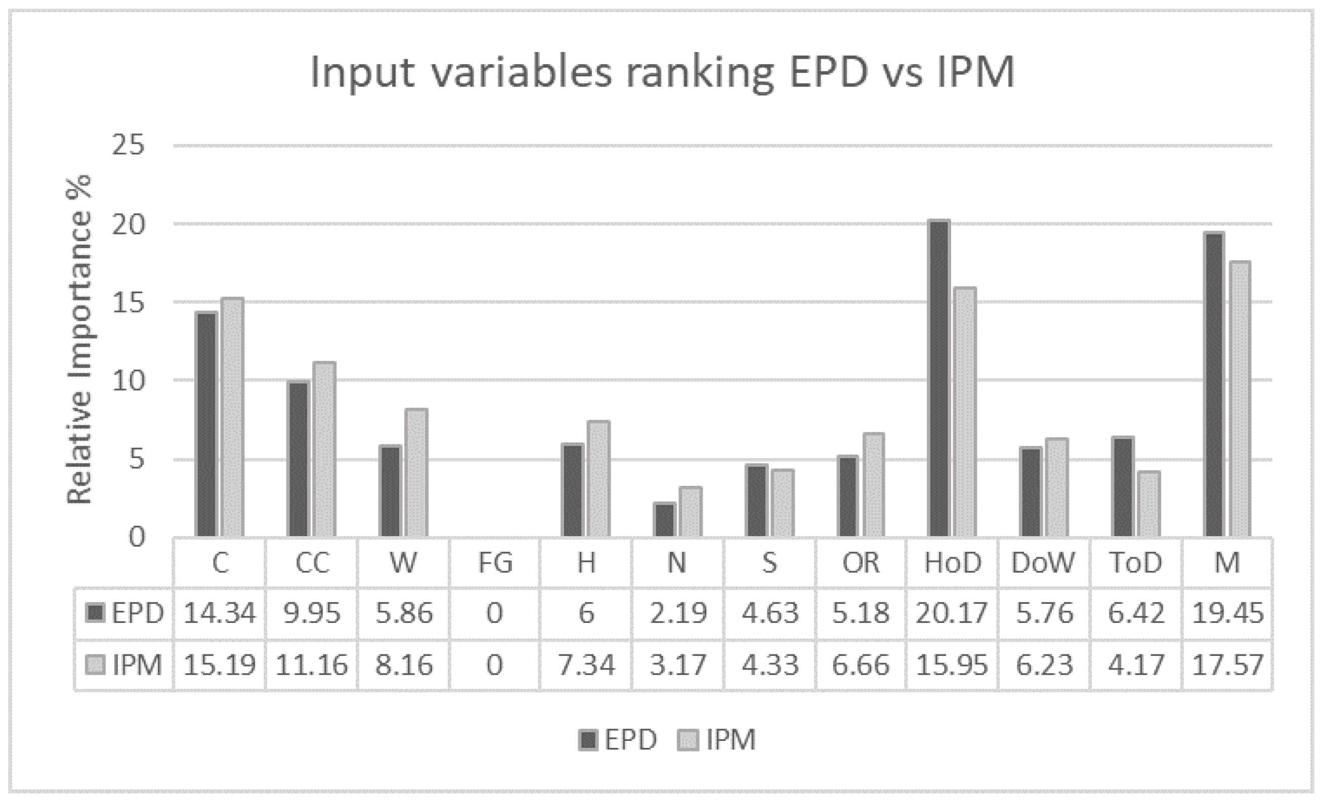
The following Figure 15 shows the relative importance of each input variable for each VIA technique, EPD and IPM.

Hour of the day (20.17% ranked first by EPD and 15.95% ranked second by IPM) and month (19.45% ranked second by EPD and 17.57% ranked first by IPM) are ranked as the most influential variables by both techniques, followed by coal (ranked third), combined cycle (ranked fourth) and wind (ranked fifth) energies. Solar (tenth) and renewable energies (ninth) are again placed as the least important predictors with the exception of Nuclear energy having, as in all simulations, a marginal contribution.

5.4. Scenario 4: VIA Full Data Set

This last scenario considers all variables in the simulation (two output and 15 input variables, Table 5), where we have incorporated the lagged prices variables (1 h, 2 h and 24 h) as predictors.

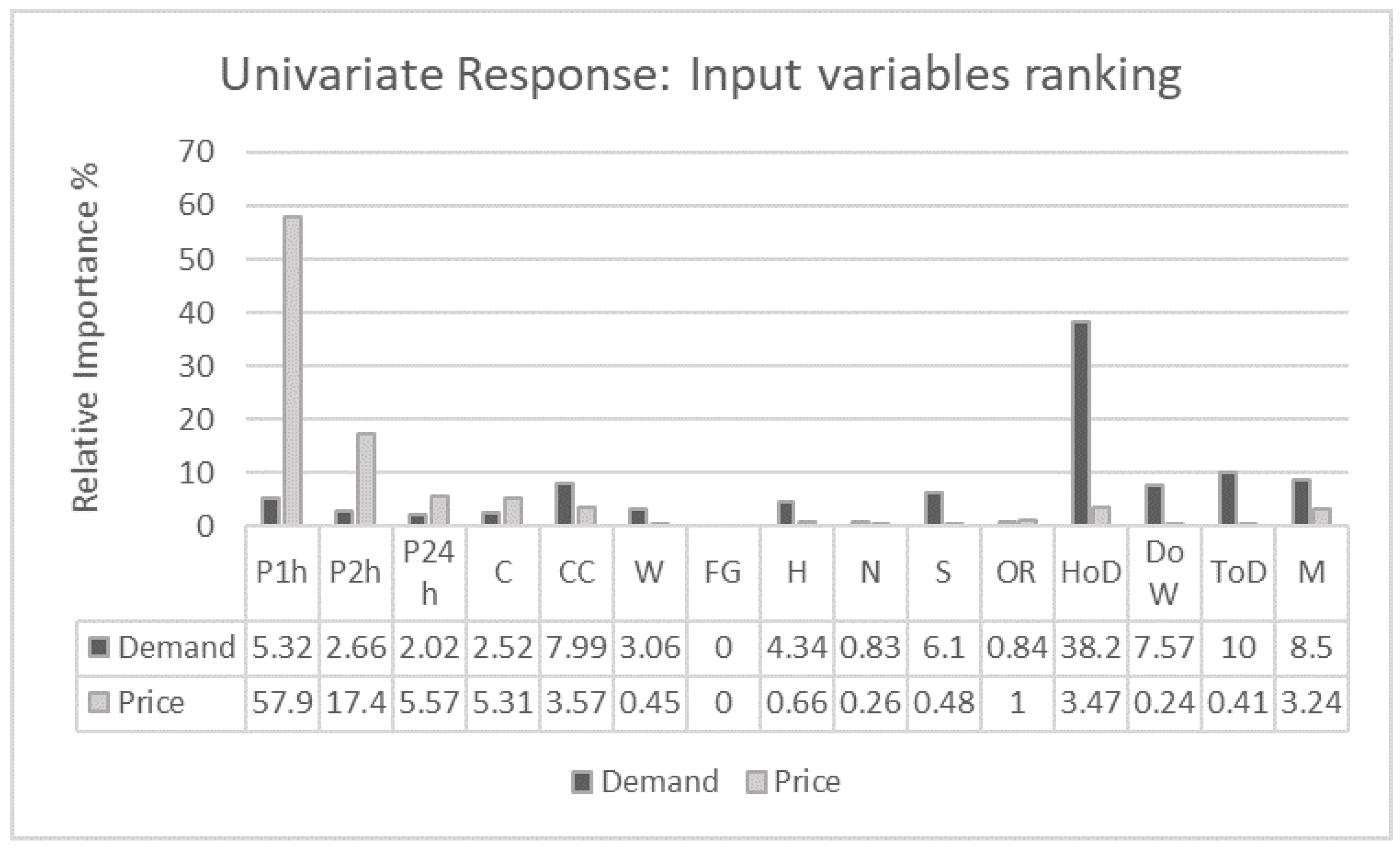
We have also computed the importance of each input variable to each of the response variables independently (The analysis has been carried out using the varimp() method (R package ‘party’)). Figure 16 shows the impact of the predictors on the demand and price when running a univariate response variable importance analysis. We see that for the price of electricity, the predictors selected (Figure 16) as important are the prices lagged one (P1h) and two hours (P2h) as well as coal (C) and combined cycle (CC) energy power, these energies being the most expensive to produce. For the demand (Figure 16), due to the normal behavior of human activity, the HoD and the rest of calendar variables have been selected as the most important predictors. To cover this demand, renewable energies are first used. For that reason, solar (S) and wind (W) power appeared also as significant, with the combined cycle (CC) and hydraulic (H) power energies selected as important in order to ensure the coverage of demand.

For the multivariate response (Demand and Price) analysis, the simulation characteristics used in the CIT algorithm to test EPD and IPM methods are: $mtry=4$ and $ntree=100$.

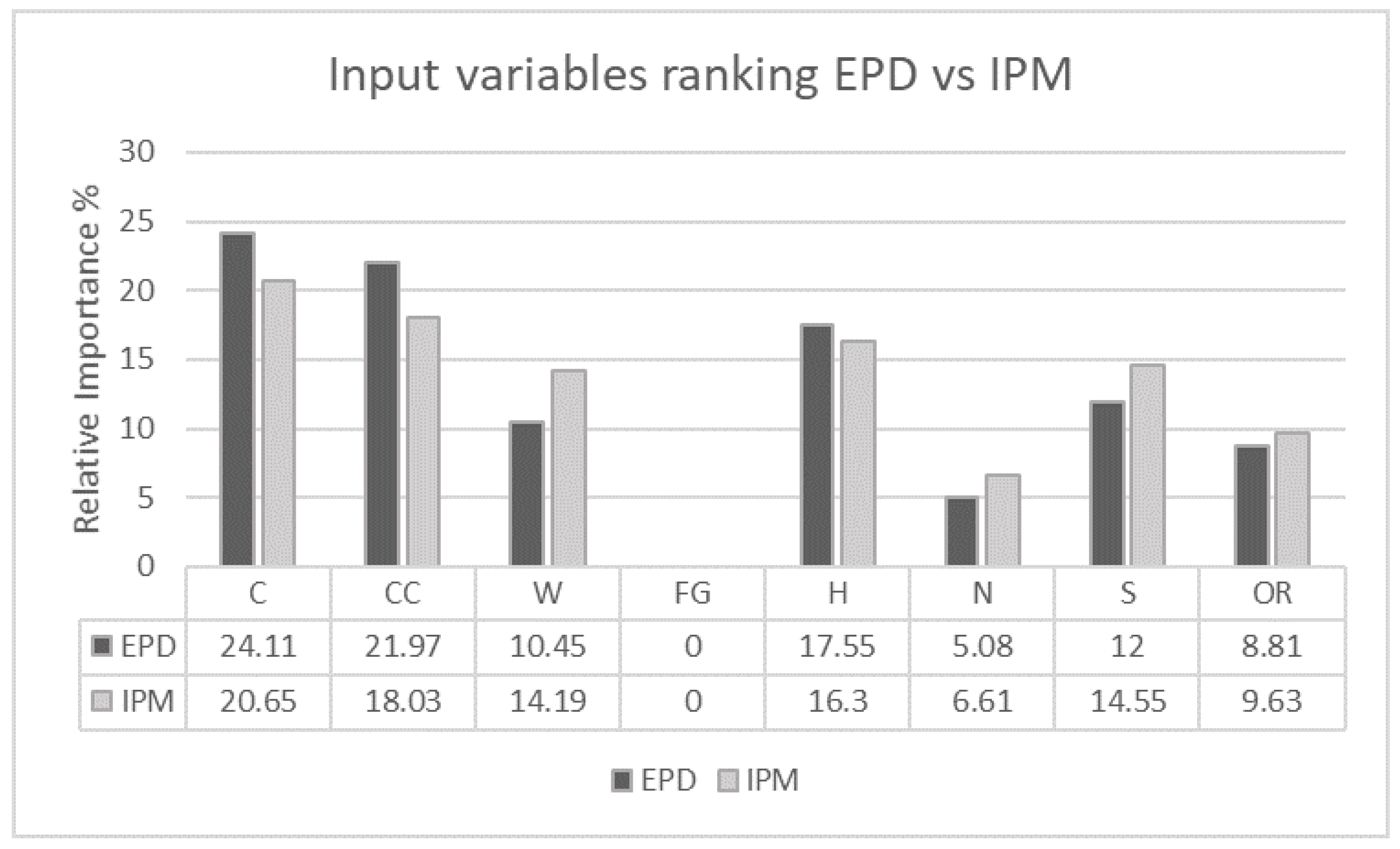
The following Figure 17 shows the relative importance of each input variable for each VIA technique, EPD, IPM and SMuRFS (SMuRFS considers as important all covariates except FG).

In general, for the multi-output VIA, the ranking patterns shown by both VIA techniques are quite analogous. Both methods, EPD and IPM, ranked the lagged price 1 h variable (P1h) in the first position, with an impact on the bivariate output of 29.38% using EPD and 21.91% for IPM, followed by the Hour of the day (HoD) variable with 18.05% and 13.93% respectively. They also consider nuclear energy (N) as the least important variable for price and demand, with a marginal contribution of 0.51% computed with EPD and 1.35% computed with IPM (fuel and gas has no impact 0.0% on the joint response).

For EPD the four most important predictors for price and demand are: lagged price 1 h (21.91%), hour of the day (18.05%), lagged price 2 h (10.12%) and month (9.58%). While the least influential input variables are nuclear energy (0.51%), followed by other renewable (1.17%), wind (2.74%) and the hydraulic energies (3.53%). A possible interpretation of these ranks could be as follows: calendar variables impact (HoD and M are in the second and fourth position respectively) are undoubtedly related to the high variability of demand of electricity (see Figure 13). For instance, different HoD (high consumption from 10:00 to 21:00 and less during the night, with repeated pattern of electricity prices Figure 12, boxplot price vs. HoD) and periods of the year (months of April, May, September and October with low demand and high in the rest) require different demand. In order to attend the high demand, renewable energies (such as solar 3.83%, eighth position) are produced, however, due to their dependence on meteorological conditions, their reliability to cover the demand is low (less controllable) and hence, more pollutant and adjustable energies such as combined cycle (CC) power (5.05%, fifth position) are produced. One of the downsides of using CC energy is the high cost of production (level of correlation between Combined cycle energy production and price of electricity is 0.68, see Figure 10). Considering this and because of the Spanish electricity market price rules (the final price is fixed at the figure at which the last producer used to cover the demand), if the demand has been covered by expensive energies, the price of electricity will also be high. This explains the high importance shown by lagged price 1 h (21.91%, first position) and 2 h (10.12%, third position) for the bivariate response.

It is also worth noting that although new environmental policies have been signed to increase the production of renewable energies, such as wind, solar and OR, these energies are still ranked in the lowest positions (12th and 13th, except solar energy which is ranked 8th).

As previously mentioned, in general, there is no direct competitor to our solution. However, Febrero et al. [32] proposed a new variable selection framework for the univariate response scenario. In their study, they selected significant predictors for the price and demand of electricity individually for the Iberian market. For the demand, their analysis showed the day-of-week indicator, price lagged 1 h ($P_{t-1}$) and combined cycle energy as the most significant factors, with renewable energies having a marginal contribution. The prediction of price had as main contributors the lagged price $P_{t-1}$, along with combined cycle and wind energies, which coincides with our solution (with the exception of wind energy generation). Again, Gonzalez et al. [31], applied a random forest variable selection method for the univariate response case. When the output variable was the price $P_{t+1}$, the hour of the day appeared as the most important variable, followed by combined cycle, hydraulic, coal energies and the demand of energy. Here again, renewable energies such as wind seem to be irrelevant for price prediction. The Reference explanatory model for price estimation (REMPE) model was used in [23] to explain the impact of input variables (previous prices, weather forecats, power generations, power demand, chronological variables, hour and weekday variables) on the hourly price of electricity in the Iberian market. The analysis in [23], concludes that price variables ($P_{t-1}$ and $P_{t-6}$), wind, cogeneration and thermal power energy generation were significant, while hour of the day and weekdays had less impact on the hourly price forecasting. In general, our solution, EPD, has some similarities with the univariate response analysis, capturing as important variables the lagged price ($P_{t-1}$), calendar effects (weekday and hour of the day) and energy production (especially the combined cycle power), with renewable energies (i.e., wind power) having non-significant contributions.

Comparing our results (multivariate response variable importance analysis, Figure 17), to those achieved in the univariate response case, papers [23,31,32], we can see that by using the new proposed algorithm EPD we can extract relevant information about variable importance, while also considering the possible interrelationships among the response variables in the analysis. This allows for a more effective analysis as there is no need to perform separate univariate studies, creating a more efficient analysis.

6. Conclusions

Identifying and analyzing the underlying factors that drive the forecasts of demand and price of electricity could reduce the uncertainty in their predictions. While the prediction of demand is comparatively more accurate than that of the price, its dependency on the capacity of renewable energy production (in order to cover the demand) and the cost of production (affecting the final price), makes it crucial to incorporate both variables, demand and price, in the analysis. Consequently, a previous variable importance analysis for the multi-output case is essential. This paper presents a new variable importance measure for multivariate output analysis, the EPD. This new method considers the possible relationships among the outputs and provides the total impact (in percentage) of each predictor on the joint response. Comparisons between EPD and other proposals, IMP and SMuRFS, show that EPD is able to measure the effect of the predictors (lagged prices, calendar effects and energy productions) on the multivariate response (price and demand of electricity of the Spanish market) more accurately (Table 1). The analysis provided by EPD (Section 5.4) showed the importance of previous lagged prices, $P_{t-1}$ and $P_{t-2}$ and calendar effects (HoD and M) on the price and demand, which could be considered to further improve the predictive accuracy of the forecasting model. The study also measured the relatively low impact of renewable energies (solar, wind and other renewable energies) compared to more pollutant ones (combined cycle and coal) despite the new Spanish environmental energy regulations. Energy participants could benefit from this methodology as a result of the previously mentioned more accurate pre-process feature selection which removes non-explanatory variables and therefore, improves the efficiency of any forecasting model. Energy traders through the new proposed methodology could improve their bidding strategies based on more accurate scenarios, which could potentially maximize their benefits by enhancing their energy production (energy suppliers) or protecting their investment strategies against high prices (buyers). On the other hand, large consumers may improve their knowledge in the market by identifying the factors that impact the price and demand fluctuations jointly, by accounting for their intrinsic relationships and hence obtaining a higher revenue. Our solution also summarizes the individual variable importance analysis which makes the computations time and data storage more efficient.

References

- Jamasb, T.; Pollitt, M. Electricity market reform in the European Union: Review of progress toward liberalization & integration. Energy J. 2005, 26, 11–41. [Google Scholar]
- Weron, R. Modeling and Forecasting Electricity Loads and Prices: A Statistical Approach; John Wiley & Sons: Hoboken, NJ, USA, 2007; Volume 403. [Google Scholar]
- Lago, J.; De Ridder, F.; Vrancx, P.; De Schutter, B. Forecasting day-ahead electricity prices in Europe: The importance of considering market integration. Appl. Energy 2018, 211, 890–903. [Google Scholar] [CrossRef] [Green Version]
- Camarero, M.; Forte, A.; Garcia-Donato, G.; Mendoza, Y.; Ordoñez, J. Variable selection in the analysis of energy consumption–growth nexus. Energy Econ. 2015, 52, 207–216. [Google Scholar] [CrossRef] [Green Version]
- Barnes, A.; Balda, J. Sizing and economic assessment of energy storage with real-time pricing and ancillary services. In Proceedings of the 2013 4th IEEE International Symposium on Power Electronics for Distributed Generation Systems (PEDG), Rogers, AR, USA, 8–11 July 2013; pp. 1–7. [Google Scholar]
- Motamedi, A.; Zareipour, H.; Rosehart, W.D. Electricity price and demand forecasting in smart grids. IEEE Trans. Smart Grid 2012, 3, 664–674. [Google Scholar] [CrossRef]
- Contreras, J.; Espinola, R.; Nogales, F.J.; Conejo, A.J. ARIMA models to predict next-day electricity prices. IEEE Trans. Power Syst. 2003, 18, 1014–1020. [Google Scholar] [CrossRef] [Green Version]
- Vilar, J.M.; Cao, R.; Aneiros, G. Forecasting next-day electricity demand and price using nonparametric functional methods. Int. J. Electr. Power Energy Syst. 2012, 39, 48–55. [Google Scholar] [CrossRef]
- Tan, Z.; Zhang, J.; Wang, J.; Xu, J. Day-ahead electricity price forecasting using wavelet transform combined with ARIMA and GARCH models. Appl. Energy 2010, 87, 3606–3610. [Google Scholar] [CrossRef]
- Carpio, J.; Juan, J.; López, D. Multivariate Exponential Smoothing and Dynamic Factor Model Applied to Hourly Electricity Price Analysis. Technometrics 2014, 56, 494–503. [Google Scholar] [CrossRef]
- Andrade, J.R.; Filipe, J.; Reis, M.; Bessa, R.J. Probabilistic Price Forecasting for Day-Ahead and Intraday Markets: Beyond the Statistical Model. Sustainability 2017, 9, 1990. [Google Scholar] [CrossRef]
- Nowotarski, J.; Weron, R. Recent advances in electricity price forecasting: A review of probabilistic forecasting. Renew. Sustain. Energy Rev. 2018, 81, 1548–1568. [Google Scholar] [CrossRef]
- Monteiro, C.; Ramirez-Rosado, I.; Fernandez-Jimenez, L.; Conde, P. Short-term price forecasting models based on artificial neural networks for intraday sessions in the iberian electricity market. Energies 2016, 9, 721. [Google Scholar] [CrossRef]
- Pino, R.; Parreno, J.; Gomez, A.; Priore, P. Forecasting next-day price of electricity in the Spanish energy market using artificial neural networks. Eng. Appl. Artif. Intell. 2008, 21, 53–62. [Google Scholar] [CrossRef]
- Weron, R. Electricity price forecasting: A review of the state-of-the-art with a look into the future. Int. J. Forecast. 2014, 30, 1030–1081. [Google Scholar] [CrossRef] [Green Version]
- Uniejewski, B.; Weron, R. Efficient forecasting of electricity spot prices with expert and LASSO models. Energies 2018, 11, 2039. [Google Scholar] [CrossRef]
- Ziel, F.; Weron, R. Day-ahead electricity price forecasting with high-dimensional structures: Univariate vs. multivariate modeling frameworks. Energy Econ. 2018, 70, 396–420. [Google Scholar] [CrossRef] [Green Version]
- Amjady, N.; Keynia, F. Electricity market price spike analysis by a hybrid data model and feature selection technique. Electr. Power Syst. Res. 2010, 80, 318–327. [Google Scholar] [CrossRef]
- Amjady, N.; Keynia, F. Day-ahead price forecasting of electricity markets by mutual information technique and cascaded neuro-evolutionary algorithm. IEEE Trans. Power Syst. 2009, 24, 306–318. [Google Scholar] [CrossRef]
- Amjady, N.; Daraeepour, A. Design of input vector for day-ahead price forecasting of electricity markets. Expert Syst. Appl. 2009, 36, 12281–12294. [Google Scholar] [CrossRef]
- Sood, R.; Koprinska, I.; Agelidis, V.G. Electricity load forecasting based on autocorrelation analysis. In Proceedings of the 2010 International Joint Conference on Neural Networks (IJCNN), Barcelona, Spain, 18–23 July 2010; pp. 1–8. [Google Scholar]
- Keynia, F. A new feature selection algorithm and composite neural network for electricity price forecasting. Eng. Appl. Artif. Intell. 2012, 25, 1687–1697. [Google Scholar] [CrossRef]
- Monteiro, C.; Fernandez-Jimenez, L.; Ramirez-Rosado, I. Explanatory information analysis for day-ahead price forecasting in the Iberian electricity market. Energies 2015, 8, 10464–10486. [Google Scholar] [CrossRef]
- González-Aparicio, I.; Zucker, A. Impact of wind power uncertainty forecasting on the market integration of wind energy in Spain. App. Energy 2015, 159, 334–349. [Google Scholar] [CrossRef] [Green Version]
- Cruz, A.; Muñoz, A.; Zamora, J.L.; Espínola, R. The effect of wind generation and weekday on Spanish electricity spot price forecasting. Electr. Power Syst. Res. 2011, 81, 1924–1935. [Google Scholar] [CrossRef]
- Ludwig, N.; Feuerriegel, S.; Neumann, D. Putting Big Data analytics to work: Feature selection for forecasting electricity prices using the LASSO and random forests. J. Decis. Syst. 2015, 24, 19–36. [Google Scholar] [CrossRef]
- Misiorek, A. Short-Term Forecasting of Electricity Prices: Do We Need a Different Model for Each Hour? Technical report; Hugo Steinhaus Center, Wroclaw University of Technology: Wroclaw, Poland, 2008. [Google Scholar]
- Karakatsani, N.V.; Bunn, D.W. Forecasting electricity prices: The impact of fundamentals and time-varying coefficients. Int. J. Forecast. 2008, 24, 764–785. [Google Scholar] [CrossRef]
- Keles, D.; Scelle, J.; Paraschiv, F.; Fichtner, W. Extended forecast methods for day-ahead electricity spot prices applying artificial neural networks. Appl. Energy 2016, 162, 218–230. [Google Scholar] [CrossRef]
- Pape, C.; Hagemann, S.; Weber, C. Are fundamentals enough? Explaining price variations in the German day-ahead and intraday power market. Energy Econ. 2016, 54, 376–387. [Google Scholar] [CrossRef] [Green Version]
- González, C.; Mira-McWilliams, J.; Juárez, I. Important variable assessment and electricity price forecasting based on regression tree models: Classification and regression trees, Bagging and Random Forests. IET Gener. Transm. Distrib. 2015, 9, 1120–1128. [Google Scholar] [CrossRef]
- Febrero-Bande, M.; González-Manteiga, W.; de la Fuente, M.O. Variable selection in functional additive regression models. In Functional Statistics and Related Fields; Springer: Berlin, Germany, 2017; pp. 113–122. [Google Scholar]
- Uniejewski, B.; Nowotarski, J.; Weron, R. Automated variable selection and shrinkage for day-ahead electricity price forecasting. Energies 2016, 9, 621. [Google Scholar] [CrossRef]
- Uniejewski, B.; Marcjasz, G.; Weron, R. Understanding Intraday Electricity Markets: Variable Selection and Very Short-Term Price Forecasting Using LASSO; Technical report; Hugo Steinhaus Center, Wroclaw University of Technology: Wroclaw, Poland, 2018. [Google Scholar]
- Koprinska, I.; Rana, M.; Agelidis, V.G. Correlation and instance based feature selection for electricity load forecasting. Knowl.-Based Syst. 2015, 82, 29–40. [Google Scholar] [CrossRef]
- George, E.I.; McCulloch, R.E. Approaches for Bayesian variable selection. Stat. Sin. 1997, 7, 339–373. [Google Scholar]
- Guyon, I.; Gunn, S.; Nikravesh, M.; Zadeh, L. (Eds.) Feature Extraction, Foundations and Applications; Series Studies in Fuzziness and Soft Computing, Physica-Verlag; Springer: Berlin, Germany, 2006. [Google Scholar]
- Archer, G.; Saltelli, A.; Sobol, I. Sensitivity measures, ANOVA-like techniques and the use of bootstrap. J. Stat. Comput. Simul. 1997, 58, 99–120. [Google Scholar] [CrossRef]
- Tibshirani, R. Regression shrinkage and selection via the lasso. J. R. Stat. Soc. Ser. B (Methodol.) 1996, 58, 267–288. [Google Scholar] [CrossRef]
- Chastaing, G.; Gamboa, F.; Prieur, C. Generalized Sobol sensitivity indices for dependent variables: Numerical methods. J. Stat. Comput. Simul. 2015, 85, 1306–1333. [Google Scholar] [CrossRef]
- Xu, L.; Lu, Z.; Xiao, S. The new importance measures based on vector projection for multivariate output: application on hydrological model. Hydrol. Earth Syst. Sci. Discuss. 2016, 2016, 1–22. [Google Scholar] [CrossRef]
- Lamboni, M.; Monod, H.; Makowski, D. Multivariate sensitivity analysis to measure global contribution of input factors in dynamic models. Reliab. Eng. Syst. Saf. 2011, 96, 450–459. [Google Scholar] [CrossRef]
- Obozinski, G.; Taskar, B.; Jordan, M.I. Joint covariate selection and joint subspace selection for multiple classification problems. Stat. Comput. 2010, 20, 231–252. [Google Scholar] [CrossRef]
- Breiman, L. Random forests. Mach. Learn. 2001, 45, 5–32. [Google Scholar] [CrossRef]
- Breiman, L. Classification and Regression Trees; Routledge: Abingdon-on-Thames, UK, 2017. [Google Scholar]
- Borchani, H.; Varando, G.; Bielza, C.; Larrañaga, P. A survey on multi-output regression. Wiley Interdiscip. Rev. Data Min. Knowl. Discov. 2015, 5, 216–233. [Google Scholar] [CrossRef] [Green Version]
- De’Ath, G. Multivariate regression trees: A new technique for modeling species–environment relationships. Ecology 2002, 83, 1105–1117. [Google Scholar]
- Kocev, D.; Vens, C.; Struyf, J.; Džeroski, S. Ensembles of multi-objective decision trees. In Proceedings of the 2007 European Conference on Machine Learning, Warsaw, Poland, 17–21 September 2007; Springer: Berlin, Germany, 2007; pp. 624–631. [Google Scholar]
- Ikonomovska, E.; Gama, J.; Džeroski, S. Incremental multi-target model trees for data streams. In Proceedings of the 2011 ACM Symposium on Applied Computing, TaiChung, Taiwan, 21–24 March 2011; ACM: New York, NY, USA, 2011; pp. 988–993. [Google Scholar]
- Hothorn, T.; Hornik, K.; Zeileis, A. Unbiased recursive partitioning: A conditional inference framework. J. Comput. Graph. Stat. 2006, 15, 651–674. [Google Scholar] [CrossRef]
- Strasser, H.; Weber, C. On the Asymptotic Theory of Permutation Statistics. Math. Methods Stat. 1999, 8, 220–250. [Google Scholar]
- Epifanio, I. Intervention in prediction measure: A new approach to assessing variable importance for random forests. BMC Bioinf. 2017, 18, 230. [Google Scholar] [CrossRef] [PubMed]
- Mayer, J.; Rahman, R.; Ghosh, S.; Pal, R. Sequential feature selection and inference using multi-variate random forests. Bioinformatics 2017, 34, 1336–1344. [Google Scholar] [CrossRef] [PubMed]
- Ishwaran, H.; Kogalur, U.B.; Gorodeski, E.Z.; Minn, A.J.; Lauer, M.S. High-dimensional variable selection for survival data. J. Am. Stat. Assoc. 2010, 105, 205–217. [Google Scholar] [CrossRef]
- Li, L.; Lu, Z.; Wu, D. A new kind of sensitivity index for multivariate output. Reliab. Eng. Syst. Saf. 2016, 147, 123–131. [Google Scholar] [CrossRef]
- Khuri, A.I.; Cornell, J.A. Response Surfaces: Designs and Analyses; CRC press: Boca Raton, FL, USA, 1996; Volume 152. [Google Scholar]
- Mara, T.A.; Tarantola, S. Variance-based sensitivity indices for models with dependent inputs. Reliab. Eng. Syst. Saf. 2012, 107, 115–121. [Google Scholar] [CrossRef]
- Red Electrica de Espana Sistema de Informacion del Operador del Sistema. Available online: https://www.esios.ree.es/es (accessed on 10 February 2018).
Figure 1.
Predictive model. Here, [price, demand] = f(). Explanatory variables: calendar effects, lagged prices and energy production variables.
Figure 2.
Hyper-parameter sensitivity analysis for the variable importance technique based on Conditional inference tree (CIT). Main effect (red): individual effect of each HP on the response. Total effects (blue): total effect of each HP when interacting with other HP on the response.
Figure 3.
Variable importance analysis (VIA) framework.
Figure 4.
mtry = 1.
Figure 5.
mtry = 4.
Figure 6.
mtry = 7.
Figure 7.
Figure 8.
Figure 9.
mtry = 8.
Figure 10.
Correlation matrix values among all continuous input variables (diagonal: demand, price, price lagged 1 h, price lagged 2 h, price lagged 24 h, coal, combined cycle, wind, fuel–gas, hydro, nuclear, solar, other renewable). (Public source: Red Eléctrica de Espana Sistema de Información del operador del sistema, www.esios.ree.es).
Figure 11.
Relative importance in % to the joint response (demand and price of electricity) of energy generation variables using the VIT Euclidean probabilistic distance (EPD) and Intervention prediction measure (IPM).
Figure 12.
Boxplot price vs. hour of the day (HoD), day of the week (DoW) (D: Sunday, J: Thursday, L: Monday, M: Tuesday, S: Saturday, V: Friday and X: Wednesday), type of day (ToD) (F: weekend, L: working day, N: holiday) and month (M). Public source: www.esios.ree.es.
Figure 13.
Boxplot Demand vs. HoD, DoW, ToD and M. Public source: www.esios.ree.es.
Figure 14.
Relative importance in % to the joint response (demand and price of electricity) of calendar variables (HoD, DoW, ToD and M) using the VIT, EPD and IPM.
Figure 15.
Relative importance in % to the joint response (demand and price of electricity) of fundamental and continuous variables using the VIT EPD and IPM.
Figure 16.
Univariate response variable importance analysis: relative importance in % of the predictors to each independent response, demand and price of electricity.
Figure 17.
Input variables ranking EPD vs. IPM.