Short-Term Electricity Price Forecasting with a Composite Fundamental-Econometric Hybrid Methodology †


Institute for Research in Technology, Technical School of Engineering (ICAI), Universidad Pontificia Comillas, 28015 Madrid, Spain
*
Author to whom correspondence should be addressed.
†
This paper is an extended version of our paper published in the EEM2018 conference on 27–29 June 2018 in Łódź, Poland.
Energies 2019, 12(6), 1067; https://doi.org/10.3390/en12061067
Submission received: 26 February 2019
/
Revised: 15 March 2019
/
Accepted: 18 March 2019
/
Published: 20 March 2019
(This article belongs to the Section F: Electrical Engineering)
Abstract
:Various power exchanges are nowadays being affected by a plethora of factors that, as a whole, cause considerable instabilities in the system. As a result, traders and practitioners must constantly adapt their strategies and look for support for their decision-making when operating in the market. In many cases, this calls for suitable electricity price forecasting models that can account for relevant aspects for electricity price forecasting. Consequently, fundamental-econometric hybrid approaches have been developed by many authors in the literature, although these have rarely been applied in short-term contexts, where other considerations and issues must be addressed. Therefore, this work aims to develop a robust hybrid methodology that is capable of making the most of the advantages fundamental and the hybrid model in a synergistic manner, while also providing insight as to how well these models perform across the year. Several methods have been utilised in this work in order to modify the hybridisation approach and the input datasets for enhanced predictive accuracy. The performance of this proposal has been analysed in the real case study of the Iberian power exchange and has outperformed other well-recognised and traditional methods.
1. Introduction
Power exchanges worldwide have undergone considerable changes since their corresponding deregulation and liberalisation events. Therefore, traders and practitioners were given more investment options in electricity markets and, as a result, these markets have grown significantly competitive and their participants are thus forced to adjust their strategies in order to withstand competition. Furthermore, there are other key factors that are important to consider, such as the rising renewable penetration and ongoing regulatory reforms.
As such, electricity price forecasting models have become greatly popular as a way of dealing with the underlying uncertainty in the market. Consequently, they are vital to several uses in this context, such as speculation, risk management and other strategic purposes. Therefore, the forecasting models must be carefully tuned in order to succeed in these applications. The first aspect that comes to mind is the planning horizon, i.e., short- medium and long-term. The literature on short-term (i.e., horizons ranging from one day to one week) forecasting models in electricity market contexts is mostly dominated by statistical or econometric approaches, whereas longer-term contexts also involve fundamental modelling of the market behaviour and dynamics [1,2,3].
Statistical and econometric approaches (e.g., time series such as ARIMA (autoregressive integrated moving average) and extensions [4,5,6,7], neural network and other AI (artificial intelligence) models [8,9,10,11], etc.) have received a considerable acceptance for many years due to their ability to capture linear (time series) and non-linear (AI) trends. Some authors have opted to merge both of these approaches into a pure econometric hybrid model in order to take advantage of both capabilities [12,13,14,15].
These models are usually trained on historical data and, thus, perform under the assumption that past behaviours in prices (apart from other explanatory factors) will replicate in the future, which is not always true in today’s evolving electricity markets. Moreover, some of these are experiencing a rather usual occurrence of extremely low or high prices. These are very important issues that cannot be underestimated and, therefore, some authors have explored other methods outside of the field of econometrics. Given that certain events such as regulatory changes or modified physical elements (e.g., transmission lines, unit decommission, etc.) in power markets are, in a considerable number of occasions, responsible for these changes with respect to the past, resorting to market fundamental models is a suitable solution.
In this context, fundamental models are aimed at the estimation of electricity prices by simulating the market clearing. To this end, a thorough representation of the system is required, including its generation units and their technical features. In this case, regulatory and other constraints can be properly set to the owners of these generation units (e.g., CO2 emissions, taxes, subsidies, etc.) in their unit commitment decisions. As a result, the estimated market prices reflect these events that cannot be easily modelled by econometrics or statistics. Nevertheless, these prices have proved to be unable to reflect short-term price dynamics (e.g., intraday patterns) [2].
Consequently, some works in the literature have proposed combining fundamental models with statistic/econometric approaches in order to make up for their weaknesses and, thus, enhance their predictive accuracy. Such hybrid models have shown positive results, especially in medium-term contexts, not only from a point forecasting perspective but also from a probabilistic point of view [3,16,17,18]. However, not as much work has been carried out in short-term applications, apart from the models of [19,20].
In addition to the low-volatile and flat price forecasts that fundamental models yield on their own, one of the main difficulties that are present in short-term applications is related to the excessively large size and resolution times in thoroughly detailed and real power systems when hourly or half-hourly arrangement is used. This issue can be lessened by performing simplifications on the structure of the system, such as aggregating generation units with similar technical features as done in [19]. Moreover, if perfect competition is considered, generation units that belong to different market agents may also be merged together, as done in [20]. However, there are no similar short-term hybrid approaches in the literature that have thoroughly modelled power exchanges with hourly precision, to the best knowledge of the authors.
Furthermore, it was observed in [20] that the contribution of the fundamental model (i.e., market clearing prices) to the econometric model increased overall accuracy. However, on particularly volatile days, the error on hours of extremely low/high prices was increased. Therefore, this calls for a forecast combination or a regime-switching model within a hybrid framework that is able to simultaneously benefit from the equilibrium price level given by the market clearing prices and the adaptability of neural network models. However, there are very few works that have addressed forecast combinations in electricity market price forecasting contexts (especially involving hybrid methods) [21,22].
Moreover, another aspect of high importance is how the hybridisation of fundamental and econometric models is performed. The most resorted procedure is, as mentioned previously, obtaining the market clearing prices from the fundamental model, which are later included in the econometric model’s input datasets. However, there are other variables that fundamental models are able to calculate, such as thermal/renewable generation outputs. Therefore, it would be interesting to study the benefits, if any, of incorporating these other variables to said datasets.
Selecting the most appropriate training period in electricity market price forecasting contexts is important albeit frequently disregarded. Statistical methods that include irregularities or structural breaks on their calibration data windows may yield higher errors and thus careful attention must be paid when selecting the input data window [23]. The authors of [24] have recently pointed out this issue and claim that forecasting models with shorter calibration windows adapt better to changes, whereas longer calibration windows result in a better estimation of the trained model’s parameters, as stated on [23]. Nevertheless, ARX (autoregressive exogenous) forecasting models are the main focus of the work presented in [24]. Therefore, this calls for a suitable procedure that can be applied to AI models, such as neural networks in order to provide a more accurate forecast.
The previously mentioned facts and suggestions encourage the electricity price forecasting model presented in this manuscript, whose contributions are summarised as follows:
- A novel short-term electricity market price forecasting model is proposed and developed, which is composed of, not only a fundamental and an econometric model, but also a unique set of combined methods that all in all contribute to an appropriate forecasting procedure.
- The fundamental model, a cost-production optimisation model, considers coal and CCGT (combined cycle gas turbine) thermal units individually and their bids were estimated based on past bids and relevant commodity prices. The econometric model is comprised of data pre-processing modules, a neural network (NN) forecasting procedure and a forecast combination approach. Data pre-processing methods involve a calibration window length selection and a similar days method.
- The hybridisation procedure of this work’s proposed fundamental-econometric hybrid forecasting model involves passing, aside from market clearing prices, thermal/hydro generation levels from the fundamental model to the econometric model.
- The proposed model has been tested on the real-size market case of the Iberian power exchange, as well as its individual components and other well-recognised models. Furthermore, several forecast combination procedures were used on the results of these models and their usefulness was assessed.
The remainder of this work is organised as follows: Section 2 describes the proposed methodology of this manuscript; Section 3 presents the results of the experiments that were performed with the proposed methodology as well as other models; and Section 4 contains the conclusions that were drawn in this work, including the suggestions for extensions and future developments of the proposed methodology.
2. Proposed Methodology
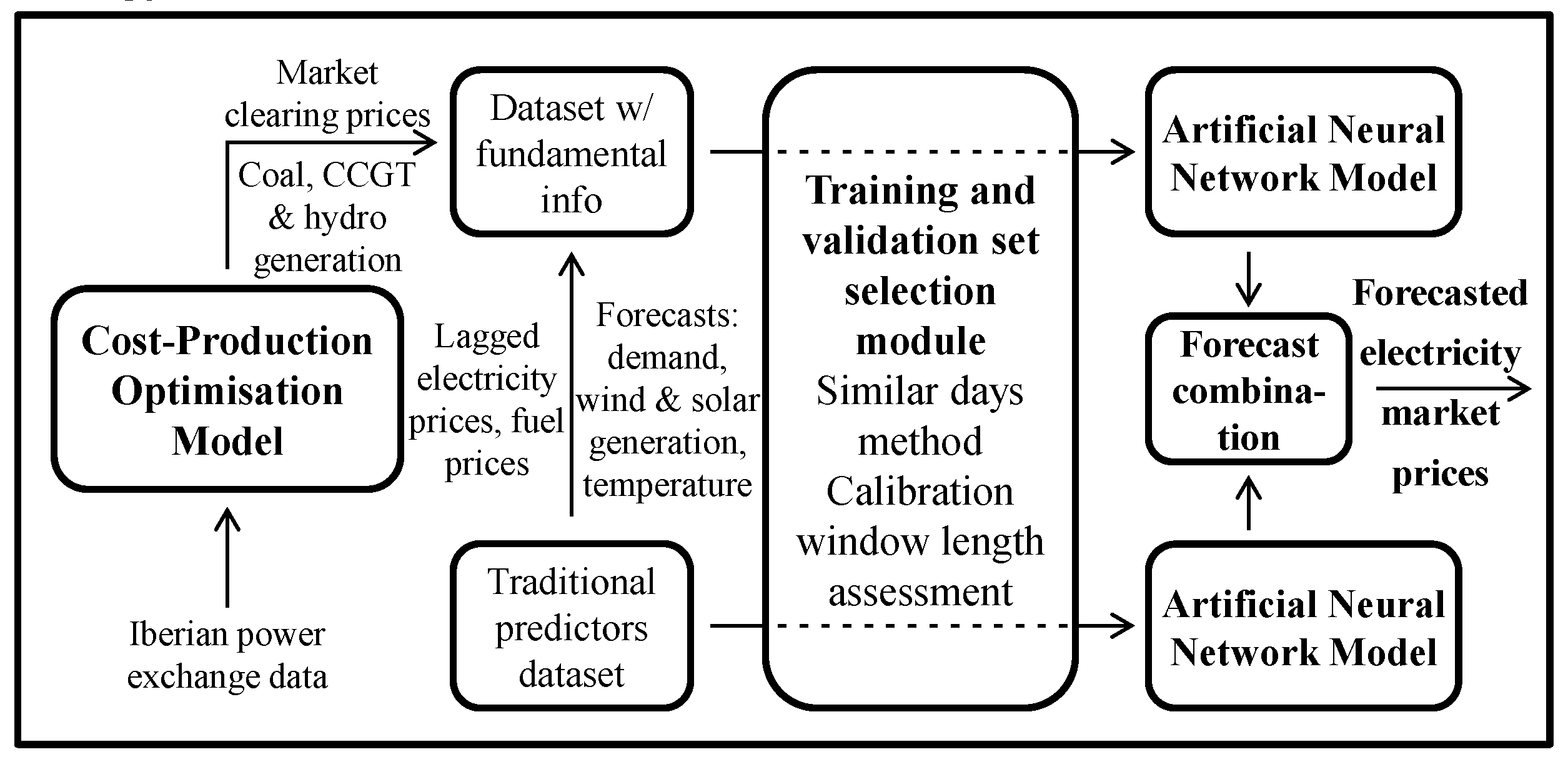
The main objective of this work is to propose and develop a novel short-term hybrid forecasting model and verify its performance on a real, full-scale and complex case study, such as the Iberian (Spain and Portugal) electricity market. A diagram of the proposed fundamental-econometric hybrid model is shown on Figure 1.
The workflow of Figure 1 runs from left to right. The fundamental model is run to obtain its corresponding output variables, which are later used as additional variables in the econometric model’s input dataset. After employing a data preprocessing approach to the input datasets, two NN models are run with and without said additional variables to finally combine the resulting sets of forecasts. The following subsections contain the specific details of each part of this work’s proposed methodology.
2.1. Fundamental Model
The fundamental component, displayed at the left-hand side of Figure 1, is composed of a cost-production optimisation model. It is based on the Iberian power exchange, whose data is available on the transparency platforms of the Spanish System Operator [25] and of the ENTSO-E (European Network of Transmission System Operators for Electricity) [26].
However, contrary to what has been done in other short-term hybrid models, such as [19,20], all CCGT and coal power units in the system were considered individually so as to verify if the resulting increase in resolution and problem size/detail is compensated by an increase in the estimated market clearing prices’ accuracy. Given the nature of the problem and its decision variables (e.g., production levels, commitment, etc.), mixed integer program (MIP) optimisation should be carried out. However, one of the aims of this work is to compute market clearing prices for later use, and thus if MIP is chosen, these prices would reflect the variable costs of only the committed units.
Therefore, the chosen nature of the corresponding optimisation problem is a relaxed MIP (i.e., RMIP) in order to account for all the generation units’ costs when simulating the market clearing as well as providing a lower resolution time. However, the resulting generation unit schedule may not be fully feasible in practice, although this poses no repercussions to the objectives of this work.
Furthermore, CCGT and coal generation unit variable costs (e.g., fuel, CO2 emissions, etc.) are being estimated based on their past bids (with at least a 90-day delay due to market confidentiality rules) and month-ahead and day-ahead forward prices of relevant commodities, such as API2 for coal and NBP for natural gas. Additionally, European CO2 emission allowances are also taken into account. This new modelling of variable costs yielded more accurate market clearing prices, as seen on Table 1.
Table 1 shows the computational differences between this work’s proposed fundamental model and that of [20] for a forecasting period of one week and a comparison of the mean absolute error (MAE, see Equation (13)) of the obtained market clearing prices throughout the year 2017:
As expected, an increase of the number of generation units in the system lead to a higher problem size, a larger maximum RAM (random-access memory) usage and a longer resolution time. However, the MAE was reduced by approximately one third with respect to the recent work of [20], which makes this increase in the level of detail and computational burden a worthwhile exchange. These results were obtained under similar conditions and a PC of similar features to those of the one indicated in [20].
2.2. Datasets and Pre-Processing Methods
As shown on Figure 1, not only the market clearing prices were taken as the output of the fundamental model, but also the generation levels of the coal, CCGT and hydro units. These were merged into a certain dataset, alongside more common predictors, which are:
- Expected values of demand, wind and solar generation.
- Expected mean temperature in the Iberian Peninsula.
- Two dummy variables indicating if it is a working day or a Sunday/holiday, thus leaving the case of Saturday for when both of these dummies are false.
- Month-ahead forward prices of API2 coal and day-ahead forward prices for NBP natural gas and European CO2 emission allowances.
- Lagged electricity market prices, specifically: one day, two days, one week and two weeks.
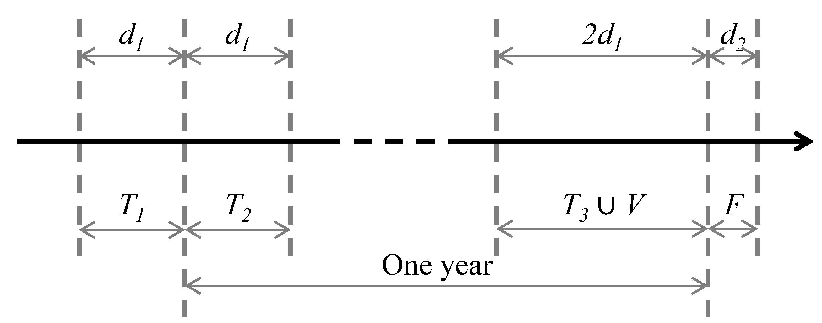
Therefore, 17 total input variables are considered in the dataset that includes the four outputs of the fundamental model. This set of input data includes all kinds of explanatory variables that influence the Iberian electricity market as per [27]. Before running the NN model with these variables, a calibration period selection procedure must be carried out so as to reduce overtraining issues in the NNs. The calibration set data of the NNs are arranged as per the timeline displayed on Figure 2, where the bottom labels indicate the interval names and the top labels the interval length in days.
Given a certain forecasting day F, the NN training set is split into three periods with their corresponding intervals in days (1y represents one year):
- T1 = (F − 1y − d1, F − 1y)
- T2 = (F − 1y, F − 1y + d1)
- T3 = (F − 2d1, F)
The length of these intervals is a function of one parameter, d1. The first two periods present relevant information pertaining to similar conditions (weather, season, etc.) in the previous year, whereas the third period contains the most recent information. However, contrary to what is usually done on NN forecasting applications, the validation period V is not placed immediately prior to day F, but anywhere within T3′s range according to a similar days method, in a similar manner to what has been carried out in the calibration period selection of [28].
The similarity test that was performed is a modified version of the similar days method proposed in [29] with the following similarity criteria: expected demand (ED), expected demand deviation (EDD), expected temperature (ET) and expected wind generation (EW). A Euclidean norm for every hour i with weighted factors is used so as to evaluate the similarity between the forecasting period F and sub-periods of equal length (i.e., of d2 days) contained in training period T3:
The weights, , are obtained via a linear regression model across every hour i that belongs to every sub-period contained in T3 (i.e., every ). This regression model is represented in the following equation:
The sub-period that presents the lowest average value of is therefore the most similar sub-period. For this work’s case, the top 20% most similar sub-periods were chosen as the validation period V. This data rearrangement is more efficient and reduces redundancy in the NN training set, as well as overfitting occurrences. Furthermore, this similar days method provides a robust control that takes calendar effects into account, such as avoiding to select non-business days as validation data when forecasting business-day prices and vice versa.
However, the length of the training set or the value of d1 should be chosen carefully. As mentioned earlier, shortened calibration windows are more appropriate in order to increase adaptability and response to sudden changes. As seen in [20], the Iberian power system on early 2017 was influenced by a highly uncommon combination of factors: very cold weather, very low hydro/wind generation, high natural gas prices and disrupted interconnection with France due to its decommissioning of nuclear power plants. Therefore, shortening calibration windows may constitute a suitable strategy during such unstable periods in order to increase forecasting accuracy.
Given that this work utilises NN models, it would be computationally cumbersome to perform an approach based on the one presented in [24], which trains an ARX-type model for several calibration windows and averages the resulting forecasts. Instead, the number of days d1 will be set according to a preliminary test based on validation set mean-square error (MSE). The MSE is calculated as per the following equation with the conventional notation ( represent the forecasted values for a certain validation period of N hours, whereas are the real values pertaining to the same period):
2.3. Neural Network Training and Forecast Procedure
In electricity price forecasting applications, one hidden layer has proven to be the most popular and appropriate option [30]. The traditional Levenberg-Marquardt algorithm is chosen for NN training, as done in many other applications in electricity price forecasting contexts, such as [8]. The hyperbolic tangent sigmoid activation function was utilised for the hidden layer’s neurons, whereas a pure linear transfer function was chosen for the output layer.
Aside from the value of d1 on unstable periods, the only parameter that must be set with regards to the NN structure is the number of neurons on its hidden layer. Given that there is no general consensus in the literature as to how many neurons should be chosen for a given number of variables, several numbers of neurons were tested (more specifically, 10 to 60 with a step of 5, which results in 11 different values). For a certain dataset and calibration period, 11 different NNs were trained, and the one that presented the lowest MSE is saved for the final NN forecast.
Furthermore, a high number of sets of forecasts for the same forecasting period were obtained using the same NN in order to account for the randomness of the initial weights of the NN training algorithm. This has been also done due to the possibility that the training algorithm may finalise upon reaching local, and not global, minima. Moreover, given that shortened training periods usually cause heightened volatility on NN forecasts, the number of replications must be set inversely proportional to the length of the calibration data.
For unstable periods, several values of d1 and NN replications were tested taking several dynamics (e.g., idiosyncratic features of prices, seasonal behaviours, etc.) into account, as displayed on Table 2.
The first ten replications of the NN models are run for each value of d1, whose resulting average validation set MSE is taken as d1 selection criterion. However, during periods of a more relative stability, the value of d1 is fixed to 30 days, due to the fact that longer calibration windows entail a better estimation when no sudden changes are present, as mentioned in [24]. Finally, the mean of the forecasted values of each replication is taken as the final forecast of the NN model.
2.4. Forecast Combination Techniques
According to Figure 1, the final step of this hybrid method involves a combination procedure, where the NN forecasts with and without fundamental information on their training datasets are combined. This is motivated due to the fact that the fundamental-econometric hybrid model of [20] yields better results on relatively stable periods (i.e., with few abrupt changes and spikes) than the pure NN model whereas the pure NN model outperforms on hours of extremely high/low prices. Therefore, it is essential to combine both of these positive effects in order to minimise the intraday adaptability reduction of the hybrid model while taking advantage of its better estimation of the equilibrium price levels.
Given that the literature regarding forecast combination in electricity price forecasting contexts does not clearly favour a specific combination method, the following methods have been tested: simple averaging, inverse validation error weighting, and Bayesian model averaging. As mentioned earlier, hourly combinations may prove useful in this application in order to assign weights. All combination methods can be represented by the following equation ( represent the forecasted values of model m for a specific hour i):
The hourly weights for each model, , differ among combination methods, but they all satisfy the usual constraints assumed in these applications, namely: ; and . Given that 2 models are considered, is equal to two. Simple averaging sets all to , which is of 1/2 in this case.
The other two combination methods are carried out for every hour of the day, which is, as mentioned earlier, due to the fact that, one model is generally more accurate when real prices are closer to their average daily value whereas the other better captures patterns related to the hours of highest and lowest prices [20].
The first hourly combination approach assigns weights inversely proportional to the square value of the forecast error, as proposed in [31]. This can be therefore applied to every hour of the days pertaining to the validation set V (represented by Vi) as follows:
The forecast error in the above equation is simply the difference between the forecast and real values in the validation set ( and respectively). For a given forecasting period F, the corresponding weights pertaining to its associated validation set V are calculated. Therefore, these weights are different for every forecasting period, which provides a certain adaptability for the combined forecasts.
The last combination method is a Bayesian model averaging (BMA) method, which is carried out in a similar hourly manner with the same validation period as input data. It is worth noting that there are only two NN models to combine, whose forecast is obtained as the mean of individual replications of their forecasting methods. Let K denote the number of individual forecasts (or replications, see Table 2) carried out in both NN models. In order to ensure feasibility in terms of resolution time, the K forecasts are divided into five subsets and their mean is later computed. As a result, ten forecasts are used for combination in the BMA method.
Let Mb denote the model space composed of these ten forecasts: Mb(b = 1, 2, …, B), B = 10. The BMA method calculates the model weights for every considered combination option among the B model forecasts as the posterior probability in the same hour i of the days in the validation period (i.e., Vi): wi,b = p(Mb|Vi). Therefore, by using the Bayes theorem, the probability density function of the BMA forecast is computed as a weighted average of the posterior distributions:
The posterior mean of the BMA forecast is represented by the following equation:
The authors of this work have implemented this combination procedure using R’s BMA package [32].
2.5. Model Performance Measures and Criteria
The forecasting performance is evaluated by means of some of the most utilised error metrics in the literature, e.g., [10], which are: mean absolute percentage error (MAPE), mean absolute error (MAE), and root-mean-square error (RMSE). These error measures for a certain period of time, N, are computed as follows:
It is worth noting that prices in the Iberian electricity market may go to zero and, thus, MAPE errors may not be appropriate for this case study. However, no actual hour with zero price values has been considered in this work’s case study.
Furthermore, a Diebold-Mariano (DM) test has been carried out in order to obtain statistically significant conclusions regarding performance comparisons. A 5% significance level has been considered, an absolute error difference as the loss differential series, and a two-sided perspective, i.e., testing for both out- and underperformance.
3. Case Studies, Results, and Discussion
This section contains the specific details regarding the case studies, as well as the results and comparisons with other electricity price forecasting models. In general, the Iberian electricity market for the entire year 2017 has been utilised as this work’s case study, as it presents several market circumstances in which the forecasting models may be put to the test. For instance, winter 2017 presents the highest standard deviation in prices ever experienced in the Iberian power exchange’s recent history, whereas summer 2017 presented relatively stable market conditions. Therefore, providing suitable performance in all of these circumstances is a highly challenging task.
According to Figure 1, the cost production model is first run in order to obtain the following outputs: market clearing prices as well as coal, CCGT and hydro unit generation outputs. This has been done for the considered training, validation and forecasting periods according to Figure 2. Regarding the NN forecasts, forecast horizons of one day in hourly resolution have been considered, i.e., d2 is considered to be of one day.
Consequently, in order to perform this work’s NN forecast for 1 January 2017, calibration data will be needed pertaining to the months of December 2015, January 2016, and December 2016. Therefore, the cost-production optimisation model must be run for the months between December 2015 and December 2017 so as to have the necessary data to perform the NN forecasts.
As it is common in the literature, e.g., [28], the forecasting models have been evaluated for every season of the year, as well as a general assessment for the whole year 2017. Given that one of the main objectives of this work is to determine the usefulness of additional output variables of the fundamental model in short-term fundamental-econometric hybrid models, two variants of this work’s proposed methodology are presented: PM1 (Proposed Model 1, only including market clearing prices) and PM2 (including also CCGT, coal and hydro generation levels).
Moreover, in order to validate this work’s hybrid models, their performance has been compared with that of six other electricity price forecasting models. The first benchmark model pertains to the fundamental-econometric hybrid model that was introduced in [20] (Benchmark 1 or BM1). The second and third benchmarks (BM2 and BM3) represent the individual price forecasting models that are used in this work’s proposed hybrid model, which are the NN and the cost-production optimisation models, respectively.
The fourth benchmark (BM4) is a linear regression model that was proposed in [33] and recently utilised in [34], which is represented by the following two equations:
In Equation (15), the log-price (day d, hour h) is calculated as a function of: lagged prices (e.g., ); the minimum log-price of the 24 h in day d minus one (i.e., ); the expected load/demand (), and three dummy variables indicating if day d is Saturday, Sunday, or Monday.
However, the Iberian electricity market has a lower price cap of zero €/MWh. Therefore, the logarithmic transform of Equation (16) is not appropriate in this case. A suitable alternative is the mirror-log transform, which has been recently applied to electricity price forecasting in [35]:
First of all, the prices were normalised as per Equation (17), which eliminates the mean in the training period T and sets the standard deviation to one. Regarding Equation (18), the parameter c was set to 1/3 as done in [35].
Benchmark five (BM5) is based on ARIMA models, which are more established and recognised in the literature. The utilised model involves a transfer function with SARIMA (seasonal ARIMA) noise, which has been developed as per the procedures presented in the works of [36,37]. Additionally, the variance of the electricity prices were stabilised by means of the Box-Cox transformation [38]. The obtained SARIMA noise’s parameters with the standard notation are represented as follows: SARIMA(1,0,0)168(1,0,2)24(1,0,0)1. Furthermore, the expected load/demand has been used as an exogenous term in this model, which thus results in a SARIMAX (SARIMA exogenous) model.
These forecasting models have been tested for every day of the year 2017. Their MAPE, MAE and RMSE errors are displayed on Table 3, Table 4 and Table 5, respectively, including the combinations between both variants of this work’s proposed model (PM1 and PM2) and the pure NN model (BM2) with the simple average, inverse error weighting and Bayesian model averaging methods (SA, IEW, and BMA, respectively).
The bold values of Table 3, Table 4 and Table 5 indicate the lowest forecasting error measures for every considered period of the year 2017. According to these results, the most accurate forecasting models seem to be BM2 on winter, PM1 on spring, PM2 on summer and the combination of PM1 + BM2 on autumn and generally during the entire year 2017.
The sixth benchmark (BM6) consists of a simple naïve approach that takes the actual electricity market prices from the previous week as the forecast:
The pure NN model (i.e., BM2) is capable of outperforming all other models in the most unstable period of 2017 thanks to its adaptability and the similar days procedure that has been paired with it. Moreover, the calibration window shortening procedure (see Table 2) also proved beneficial, reducing winter MAE by 0.7 €/MWh approximately. However, incorporating fundamental-related variables to this NN model yields a lower forecasting error on all other periods.
The difference between PM1 and PM2 indicates the benefits and drawbacks of incorporating additional variables from the fundamental model (i.e., market clearing prices alone, PM1, or also hydro/thermal generation levels, PM2). The highest error differences can be seen between spring and summer. Additionally, model PM1 seems to outperform on the other two seasons and on the entire year 2017. This suggests that the price formation in summer is more characterised by market fundamentals and thus the contribution provided by the fundamental model is more advantageous.
Moreover, the hybridisation approach of PM1 between the fundamental model and the NN model reduces overall forecasting error as a result of the synergy between the adaptability of the NN model and the equilibrium price level provided by the fundamental model. Regarding the forecast combinations between both variants of the proposed model and BM2, they do not seem to provide lower errors on some specific periods of the year 2017 (when compared to both individual models prior to the combination), but they do when considering the entire year 2017, which is mainly due to the results in autumn. The accuracy improvement as a result of the combination confirm the statements made in [20] and the previously mentioned synergy.
Furthermore, the results for every combination method seem to indicate that the simple average is most beneficial, although closely followed by the inverse error weighting procedure. As in other works in the same forecasting context [21], the simple average method seems to be challenging to outperform, even with more sophisticated methods.
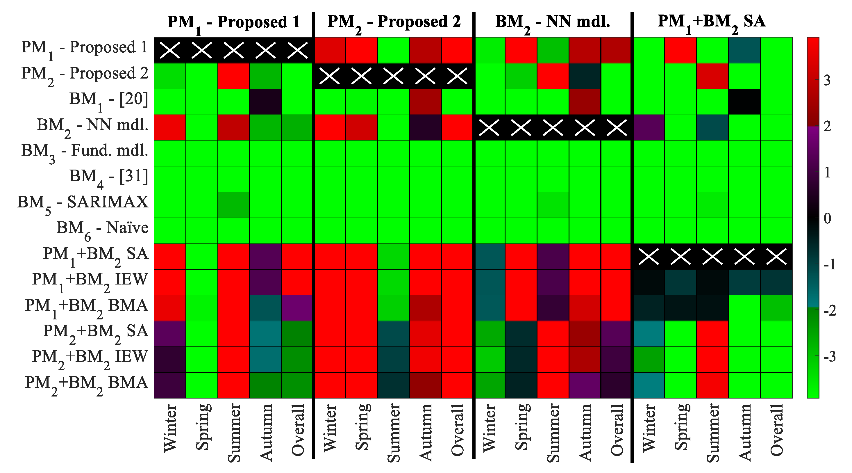
Moreover, a DM test is carried out in order to verify the statistical significance of these error measures. Figure 3 shows the DM test results for the most outperforming models. Its colour-bar indicates the value of the DM test statistic that assesses if the model on the top header significantly outperforms the model on the left header. Given that this test is run with a 5% significance level, the corresponding critical value is of 1.96. Therefore:
- DM statistic < −1.96 implies significant outperformance
- DM statistic > 1.96 implies significant underperformance
- Otherwise no significant out- or underperformance
According to Figure 3, model PM1 is the most outperforming model during spring and shows suitable overall performance when considering the entire year 2017. It is also one of the few models not significantly bested by the hybrid model of [20] (i.e., BM1) during autumn. Regarding model PM2, it is not significantly outperformed by any other model during summer, but shows an otherwise slight underachievement when tested against PM1.
The most remarkable model on the winter is the pure NN model, although its combinations with PM1 are almost significantly bested by it. Furthermore, the simple average method between PM1 and BM2 seems to generally outperform every other model when considering the whole year 2017.
4. Conclusions
The proposal detailed in this work is based on a novel methodology that is composed of a hybrid fundamental-econometric electricity market price forecasting model. The individual forecasting models of this procedure have been coupled by utilising several variables, such as the market clearing price, of the cost-production optimisation model as input data of the neural network model.
In order to reduce overfitting, the neural network training method involved a validation period selection via a similar day’s method. Moreover, on unstable periods, a calibration period shortening procedure based on validation set error was carried out. Finally, the forecasts from the hybrid model and the NN model were combined in order to provide the final forecast of this work’s proposal. The following observations and findings summarise the conclusions drawn in this work:
- The proposed hybrid model is capable of simultaneously benefitting from the NN model’s adjustability for sudden price changes and from the equilibrium price level provided by fundamental-related information.
- Highly unstable periods, such as early 2017, can be dealt with shortened calibration windows in order to further increase adaptability for NN model forecasts.
- On periods of more relative stability, such as summer 2017, electricity market price behaviours are responding more to market fundamentals and, thus, incorporating additional variables to the hybrid model, such as thermal/hydro generation levels, proves advantageous.
- On the other periods and generally throughout 2017, a simple average combination procedure between the hybrid model and the pure NN model further reduces forecasting error, providing a heightened and better balanced synergy between the considered fundamental and econometric approaches.
All in all, the unique set of methodologies that constitute this work’s proposed hybrid forecasting model has demonstrated a suitable performance for short-term electricity market price forecasting in the case of the Iberian electricity power exchange throughout the year 2017, while also outperforming other benchmark models.
However, some of the methodologies employed in this work may be modified or extended in order to explore any potential improvement, such as, for example, a more optimal forecast combination method or a similar days method based on additional or different criteria.
Author Contributions
Conceptualization: R.A.d.M., A.B., and J.R.; data curation: R.A.d.M.; formal analysis: R.A.d.M.; investigation: R.A.d.M.; methodology: R.A.d.M., A.B., and J.R.; software: R.A.d.M.; supervision: A.B. and J.R.; validation: R.A.d.M. and A.B.; visualization: R.A.d.M.; writing—original draft: R.A.d.M. and A.B.; writing—review and editing: R.A.d.M., A.B., and J.R.
Funding
This research received no external funding.
Conflicts of Interest
The authors declare no conflict of interest.
References
- Weron, R. Electricity price forecasting: A review of the state-of-the-art with a look into the future. Int. J. Forecast. 2014, 30, 1030–1081. [Google Scholar] [CrossRef] [Green Version]
- Bello, A.; Reneses, J.; Muñoz, A.; Delgadillo, A. Probabilistic forecasting of hourly electricity prices in the medium-term using spatial interpolation techniques. Int. J. Forecast. 2016, 32, 966–980. [Google Scholar] [CrossRef]
- Bello, A.; Bunn, D.W.; Reneses, J.; Munoz, A. Medium-Term Probabilistic Forecasting of Electricity Prices: a Hybrid Approach. IEEE Trans. Power Syst. 2016, 32, 334–343. [Google Scholar] [CrossRef]
- Contreras, J.; Espínola, R.; Nogales, F.J.; Conejo, A.J. ARIMA models to predict next-day electricity prices. IEEE Trans. Power Syst. 2003, 18, 1014–1020. [Google Scholar] [CrossRef] [Green Version]
- Cruz, A.; Muñoz, A.; Zamora, J.L.; Espínola, R. The effect of wind generation and weekday on Spanish electricity spot price forecasting. Electr. Power Syst. Res. 2011, 81, 1924–1935. [Google Scholar] [CrossRef]
- García-Martos, C.; Rodríguez, J.; Sánchez, M.J. Modelling and forecasting fossil fuels, CO2 and electricity prices and their volatilities. Appl. Energy. 2013, 101, 363–375. [Google Scholar] [CrossRef]
- Sánchez De La Nieta, A.A.; González, V.; Contreras, J. Portfolio decision of short-term electricity forecasted prices through stochastic programming. Energies 2016, 9, 69. [Google Scholar] [CrossRef]
- Catalão, J.P.S.; Mariano, S.J.P.S.; Mendes, V.M.F.; Ferreira, L.A.F.M. Short-term electricity prices forecasting in a competitive market: A neural network approach. Electr. Power Syst. Res. 2007, 77, 1297–1304. [Google Scholar] [CrossRef] [Green Version]
- Keles, D.; Scelle, J.; Paraschiv, F.; Fichtner, W. Extended forecast methods for day-ahead electricity spot prices applying artificial neural networks. Appl. Energy 2016, 162, 218–230. [Google Scholar] [CrossRef]
- Sandhu, H.S.; Fang, L.; Guan, L. Forecasting day-ahead price spikes for the Ontario electricity market. Electr. Power Syst. Res. 2016, 141, 450–459. [Google Scholar] [CrossRef]
- Monteiro, C.; Ramirez-Rosado, I.J.; Fernandez-Jimenez, L.A.; Conde, P. Short-term price forecasting models based on artificial neural networks for intraday sessions in the Iberian electricity market. Energies 2016, 9, 721. [Google Scholar] [CrossRef]
- Amjady, N.; Daraeepour, A.; Keynia, F. Day-ahead electricity price forecasting by modified relief algorithm and hybrid neural network. IET Gener. Transm. Distrib. 2010, 4, 432. [Google Scholar] [CrossRef]
- Yan, X.; Chowdhury, N.A. Mid-term electricity market clearing price forecasting using multiple support vector machine. IET Gener. Transm. Distrib. 2014, 8, 1572–1582. [Google Scholar] [CrossRef]
- Chaâbane, N. A hybrid ARFIMA and neural network model for electricity price prediction. Int. J. Electr. Power Energy Syst. 2014, 55, 187–194. [Google Scholar] [CrossRef]
- Yang, Z.; Ce, L.; Lian, L. Electricity price forecasting by a hybrid model, combining wavelet transform, ARMA and kernel-based extreme learning machine methods. Appl. Energy 2017, 190, 291–305. [Google Scholar] [CrossRef]
- Karakatsani, N.V.; Bunn, D.W. Forecasting electricity prices: The impact of fundamentals and time-varying coefficients. Int. J. Forecast. 2008, 24, 764–785. [Google Scholar] [CrossRef]
- Bello, A.; Bunn, D.; Reneses, J.; Muñoz, A. Parametric Density Recalibration of a Fundamental Market Model to Forecast Electricity Prices. Energies 2016, 9, 959. [Google Scholar] [CrossRef]
- Nowotarski, J.; Weron, R. Recent advances in electricity price forecasting: A review of probabilistic forecasting. Renew. Sustain. Energy Rev. 2017. [Google Scholar] [CrossRef]
- González, V.; Contreras, J.; Bunn, D.W. Forecasting power prices using a hybrid fundamental-econometric model. IEEE Trans. Power Syst. 2012, 27, 363–372. [Google Scholar] [CrossRef]
- De Marcos, R.A.; Bello, A.; Reneses, J. Electricity price forecasting in the short term hybridising fundamental and econometric modelling. Electr. Power Syst. Res. 2019, 167, 240–251. [Google Scholar] [CrossRef]
- Bordignon, S.; Bunn, D.W.; Lisi, F.; Nan, F. Combining day-ahead forecasts for British electricity prices. Energy Econ. 2013, 35, 88–103. [Google Scholar] [CrossRef] [Green Version]
- Nowotarski, J.; Raviv, E.; Trück, S.; Weron, R. An empirical comparison of alternative schemes for combining electricity spot price forecasts. Energy Econ. 2014, 46, 395–412. [Google Scholar] [CrossRef]
- Pesaran, M.H.; Timmermann, A. Selection of estimation window in the presence of breaks. J. Econom. 2007, 137, 134–161. [Google Scholar] [CrossRef] [Green Version]
- Marcjasz, G.; Serafin, T.; Weron, R. Selection of calibration windows for day-ahead electricity price forecasting. Energies 2018, 11, 2364. [Google Scholar] [CrossRef]
- Transparency Platform of the Spanish System Operator. Available online: https://www.esios.ree.es/en (accessed on 13 November 2018).
- Transparency Platform of the ENTSO-E. Available online: https://transparency.entsoe.eu/ (accessed on 11 September 2018).
- Monteiro, C.; Fernandez-Jimenez, L.A.; Ramirez-Rosado, I.J. Explanatory information analysis for day-ahead price forecasting in the Iberian electricity market. Energies 2015, 8, 10464–10486. [Google Scholar] [CrossRef]
- Bento, P.M.R.; Pombo, J.A.N.; Calado, M.R.A.; Mariano, S.J.P.S. A bat optimized neural network and wavelet transform approach for short-term price forecasting. Appl. Energy 2018, 210, 88–97. [Google Scholar] [CrossRef]
- Mandal, P.; Senjyu, T.; Funabashi, T. Neural networks approach to forecast several hour ahead electricity prices and loads in deregulated market. Energy Convers. Manag. 2006, 47, 2128–2142. [Google Scholar] [CrossRef]
- Bello, A.; Reneses, J.; Muñoz, A. Medium-term probabilistic forecasting of extremely low prices in electricity markets: Application to the Spanish case. Energies 2016, 9, 193. [Google Scholar] [CrossRef]
- Bates, J.M.; Granger, C.W.J. The Combination of Forecasts. J. Oper. Res. 1969, 20, 451–468. [Google Scholar] [CrossRef]
- Raftery, A.E.; Painter, I.S.; Volinsky, C.T. BMA: An R package for Bayesian Model Averaging. R News 2005, 5, 2–8. [Google Scholar] [CrossRef]
- Weron, R.; Misiorek, A. Short-Term Electricity Price Forecasting with Time Series Models: A Review and Evaluation. In Complex Electricity Markets; IEPŁ & SEP: Łódź, Poland, 2006; pp. 231–254. [Google Scholar]
- Uniejewski, B.; Nowotarski, J.; Weron, R. Automated variable selection and shrinkage for day-ahead electricity price forecasting. Energies 2016, 9, 621. [Google Scholar] [CrossRef]
- Uniejewski, B.; Weron, R.; Ziel, F. Variance stabilizing transformations for electricity spot price forecasting. IEEE Trans. Power Syst. 2018, 33, 2219–2229. [Google Scholar] [CrossRef]
- Box, G.; Jenkins, G. Time Series Analysis—Forecasting and Control; Holden Day: San Francisco, CA, USA, 1970. [Google Scholar] [CrossRef]
- Pankratz, A. Building Dynamic Regression Models: Model Identification. In Forecasting with Dynamic Regression Models; John Wiley & Sons: Hoboken, NJ, USA, 2012; Volume 935, pp. 167–201. [Google Scholar] [CrossRef]
- Box, G.E.P.; Cox, D.R. An analysis of transformations. J. R. Stat. Soc. Ser. B 1964, 26, 211–252. [Google Scholar] [CrossRef]
Figure 1.
Overview of the proposed fundamental-econometric model.

Figure 2.
Training, validation, and test/forecast periods arrangement.

Figure 3.
DM test for PM1, PM2, BM2 and simple average of PM1 + BM2.


Table 1.
Comparison of computational statistics and MAE of the market clearing prices estimated by the fundamental model.
Table 1.
Comparison of computational statistics and MAE of the market clearing prices estimated by the fundamental model.
| Model | Equations | Variables | Runtime | Max. RAM | 2017 MAE |
|---|---|---|---|---|---|
| Proposed | 50,745 | 118,905 | 7.40 s | 278 MB | 6.84 €/MWh |
| [20] | 12,440 | 71,024 | 3.91 s | 76 MB | 10.31 €/MWh |
Table 2.
Training and validation sets for NN forecasting on unstable periods.
| d1 | T1 ∪ T2 ∪ T3 ∪ V | V | No. of NN Replications |
|---|---|---|---|
| 30 days | 120 days | 12 days | 50 |
| 15 days | 60 days | 6 days | 75 |
| 10 days | 40 days | 4 days | 85 |
| 5 days | 20 days | 2 days | 100 |
Table 3.
Forecasting error in terms of MAPE (%).
| Model | Winter | Spring | Summer | Autumn | Average |
|---|---|---|---|---|---|
| PM1 − Proposed 1 | 11.40 | 7.377 | 4.746 | 6.689 | 7.534 |
| PM2 − Proposed 2 | 11.68 | 8.106 | 4.450 | 6.812 | 7.744 |
| BM1 − [20] | 12.83 | 8.840 | 5.016 | 6.764 | 8.341 |
| BM2 − NN mdl. | 11.12 | 7.804 | 4.605 | 6.834 | 7.575 |
| BM3 − Fund. mdl. | 20.47 | 13.60 | 10.99 | 10.58 | 13.88 |
| BM4 − [33] | 16.79 | 13.58 | 7.153 | 10.51 | 11.99 |
| BM5 − SARIMAX | 15.06 | 9.293 | 5.097 | 7.654 | 9.248 |
| BM6 − Naïve | 25.93 | 17.55 | 9.343 | 12.82 | 16.37 |
| PM1 + BM2 SA | 11.21 | 7.488 | 4.584 | 6.645 | 7.464 |
| PM1 + BM2 IEW | 11.21 | 7.490 | 4.584 | 6.645 | 7.465 |
| PM1 + BM2 BMA | 11.20 | 7.475 | 4.586 | 6.722 | 7.478 |
| PM2 + BM2 SA | 11.30 | 7.902 | 4.477 | 6.756 | 7.591 |
| PM2 + BM2 IEW | 11.33 | 7.905 | 4.475 | 6.751 | 7.597 |
| PM2 + BM2 BMA | 11.36 | 7.924 | 4.470 | 6.774 | 7.615 |
Table 4.
Forecasting error in terms of MAE (€/MWh).
| Model | Winter | Spring | Summer | Autumn | Average |
|---|---|---|---|---|---|
| PM1 − Proposed 1 | 4.641 | 2.641 | 2.197 | 3.350 | 3.199 |
| PM2 − Proposed 2 | 4.756 | 2.882 | 2.070 | 3.453 | 3.282 |
| BM1 − [20] | 5.137 | 3.068 | 2.359 | 3.331 | 3.465 |
| BM2 − NN mdl. | 4.562 | 2.826 | 2.136 | 3.440 | 3.233 |
| BM3 − Fund. mdl. | 10.81 | 5.696 | 5.066 | 5.872 | 6.842 |
| BM4 − [33] | 6.838 | 4.765 | 3.262 | 5.066 | 4.972 |
| BM5 − SARIMAX | 8.113 | 4.150 | 2.473 | 4.454 | 4.780 |
| BM6 − Naïve | 10.53 | 6.225 | 4.266 | 6.387 | 6.828 |
| PM1 + BM2 SA | 4.577 | 2.690 | 2.123 | 3.329 | 3.172 |
| PM1 + BM2 IEW | 4.577 | 2.691 | 2.123 | 3.330 | 3.172 |
| PM1 + BM2 BMA | 4.583 | 2.693 | 2.125 | 3.376 | 3.186 |
| PM2 + BM2 SA | 4.610 | 2.832 | 2.079 | 3.409 | 3.224 |
| PM2 + BM2 IEW | 4.624 | 2.831 | 2.078 | 3.406 | 3.227 |
| PM2 + BM2 BMA | 4.618 | 2.831 | 2.077 | 3.418 | 3.228 |
Table 5.
Forecasting error in terms of RMSE (€/MWh).
| Model | Winter | Spring | Summer | Autumn | Average |
|---|---|---|---|---|---|
| PM1 − Proposed 1 | 5.415 | 3.134 | 2.651 | 4.022 | 3.796 |
| PM2 − Proposed 2 | 5.479 | 3.407 | 2.517 | 4.129 | 3.874 |
| BM1 − [20] | 5.921 | 3.658 | 2.840 | 4.003 | 4.096 |
| BM2 − NN mdl. | 5.308 | 3.342 | 2.588 | 4.089 | 3.823 |
| BM3 − Fund. mdl. | 12.19 | 6.685 | 5.759 | 7.158 | 7.927 |
| BM4 − [33] | 7.809 | 5.552 | 3.885 | 6.055 | 5.814 |
| BM5 − SARIMAX | 10.84 | 5.585 | 4.531 | 4.959 | 6.460 |
| BM6 − Naïve | 11.48 | 7.092 | 5.030 | 7.567 | 7.773 |
| PM1 + BM2 SA | 5.337 | 3.194 | 2.575 | 3.986 | 3.764 |
| PM1 + BM2 IEW | 5.338 | 3.194 | 2.575 | 3.986 | 3.764 |
| PM1 + BM2 BMA | 5.349 | 3.207 | 2.583 | 4.032 | 3.783 |
| PM2 + BM2 SA | 5.334 | 3.349 | 2.525 | 4.069 | 3.810 |
| PM2 + BM2 IEW | 5.350 | 3.349 | 2.524 | 4.066 | 3.813 |
| PM2 + BM2 BMA | 5.359 | 3.356 | 2.523 | 4.092 | 3.823 |
© 2019 by the authors. Licensee MDPI, Basel, Switzerland. This article is an open access article distributed under the terms and conditions of the Creative Commons Attribution (CC BY) license (http://creativecommons.org/licenses/by/4.0/).
Share and Cite
MDPI and ACS Style
de Marcos, R.A.; Bello, A.; Reneses, J. Short-Term Electricity Price Forecasting with a Composite Fundamental-Econometric Hybrid Methodology. Energies 2019, 12, 1067. https://doi.org/10.3390/en12061067
AMA Style
de Marcos RA, Bello A, Reneses J. Short-Term Electricity Price Forecasting with a Composite Fundamental-Econometric Hybrid Methodology. Energies. 2019; 12(6):1067. https://doi.org/10.3390/en12061067
Chicago/Turabian Stylede Marcos, Rodrigo A., Antonio Bello, and Javier Reneses. 2019. "Short-Term Electricity Price Forecasting with a Composite Fundamental-Econometric Hybrid Methodology" Energies 12, no. 6: 1067. https://doi.org/10.3390/en12061067
Note that from the first issue of 2016, this journal uses article numbers instead of page numbers. See further details here.