Unsteadiness of Tip Leakage Flow in the Detached-Eddy Simulation on a Transonic Rotor with Vortex Breakdown Phenomenon


Institute of Gas Turbine, Department of Energy and Power Engineering, Tsinghua University, Beijing 100084, China
*
Author to whom correspondence should be addressed.
Energies 2019, 12(5), 954; https://doi.org/10.3390/en12050954
Submission received: 22 January 2019
/
Revised: 22 February 2019
/
Accepted: 7 March 2019
/
Published: 12 March 2019
(This article belongs to the Special Issue Fluid Flow and Heat Transfer)
Abstract
:Tip leakage vortex (TLV) in a transonic compressor rotor was investigated numerically using detached-eddy simulation (DES) method at different working conditions. Strong unsteadiness was found at the tip region, causing a considerable fluctuation in total pressure distribution and flow angle distribution above 80% span. The unsteadiness at near choke point and peak efficiency point is not obvious. DES method can resolve more detailed flow patterns than RANS (Reynolds-averaged Navier–Stokes) results, and detailed structures of the tip leakage flow were captured. A spiral-type breakdown structure of the TLV was successfully observed at the near stall point when the TLV passed through the bow shock. The breakdown of TLV contributed to the unsteadiness and the blockage effect at the tip region.
1. Introduction
Driven by the pressure gradient inside the clearance of the rotor and casing, tip leakage is an unavoidable phenomenon in the field of turbomachinery, which scholars have studied for a long time in both compressible [1,2,3,4] and incompressible [5,6,7,8] fields. As for axial compressors, tip leakage flow plays an even more significant role due to its close relationship with loss and stall characteristics [9,10], which are highly valued in the design or analyzing processes. Aiming at reducing the impact of tip leakage flow, plenty of flow control methods (such as air injection [11], bleeding [12], casing treatment [13] and plasma actuation [14]) have been studied in recent years.
As for low-speed compressors, flow structures as well as unsteadiness of tip leakage vortex (TLV) have been widely studied and certain achievements were obtained through numerical efforts and experiments. As the flow coefficient decreases, the interface between the TLV and the incoming flow moves upstream [15], and the trajectory of which will be aligned with the leading edge when the rotor finally encounters a spike-type stall inception [16]. The criterion for spike-initiated numerical stall that leading-edge spillage and trailing-edge backflow are both essential was proved effective in low-speed compressor experiments [17]. Leading-edge spillage was later found to be an accompanying phenomenon, whose fundamental cause is probably the tornado-like vortex, resulted from the interaction between TLV and leading-edge separation [18]. In rotors with a large gap, attention was also paid to the effects of double-leakage tip clearance flow, which generates a vortex rope and subsequent extra mixing loss in the adjacent blade passage [19]. With the increase of stage loading, the importance of tip leakage flow in high-speed or transonic compressor has been increasingly emphasized. There are indeed similarities in the basic structures and mechanisms of the TLV in low-speed compressors and transonic ones. Nevertheless, conclusions for tip leakage flow in low-speed compressors are not entirely suitable for transonic ones, due to further larger pressure gradient and the existence of shock wave. When the TLV crosses the shock, it interacts both with the shock wave and with the pressure-side secondary flows generating a leakage-interaction-region of low speed, high entropy and high turbulence [2]. The interaction results in extra complexity and less stability in the tip flow field, which is considered a hot spot. Strong self-induced unsteadiness was found in the TLV with a characteristic frequency near 60% BPF (blade passing frequency) [4,20,21] and the oscillation of passage shock was revealed as well [22]. Moreover, the casing boundary layer along with the blade surface boundary layer may participate in the interacting process [23], especially at near stall point where a shock-induced separation inside the boundary layer is likely to happen in most cases. Under these circumstances, the TLV and its interaction can make a great impact on the overall performance and eventually lead to a spike-type stall inception in transonic compressors [24].
Despite the considerable efforts made by scholars in turbomachinery community, the complete mechanism of TLV and its influence on the tip flow field are still not fully understood, especially in transonic compressors. Previous investigations have shown that the interaction between the shock and TLV contributes a lot to the unsteadiness in the tip flow field, but failed to reveal this interacting process in detail. On the other hand, Reynolds-averaged Navier–Stokes (RANS) method is routinely adopted in most simulations among previous studies; however, traditional turbulence models have native defects in predicting the unsteady and vortical flows such as the TLV [25]. As a result, DES (detached-eddy simulation) method is thought to be an alternative in capturing separated or vortical flow with bearable cost [26]. Up to now, many scholars [18,27,28,29,30] have applied DES methods to the turbomachinery field and achieved satisfactory results.
In this paper, we carried out DES investigations of a transonic compressor rotor, focused on the structure of the TLV, the interaction with shock wave as well as the unsteady characteristics. Due to the limits of computing resources, a single-row DES calculation was adopted. This paper is organized as follows: the compressor and the numerical method chosen in the present study are demonstrated in Section 2, with the validation results shown in Section 3.1. Section 3.2 mainly deals with the unsteadiness related to the TLV. Detailed structures of the TLV at different working conditions are shown in Section 3.3, focused on the vortex breakdown phenomenon at near stall point. Section 4 mainly deals with the mechanism of leakage vortex breakdown. Finally, a short conclusion is drawn in Section 5.
2. Methodology
2.1. Testing Case
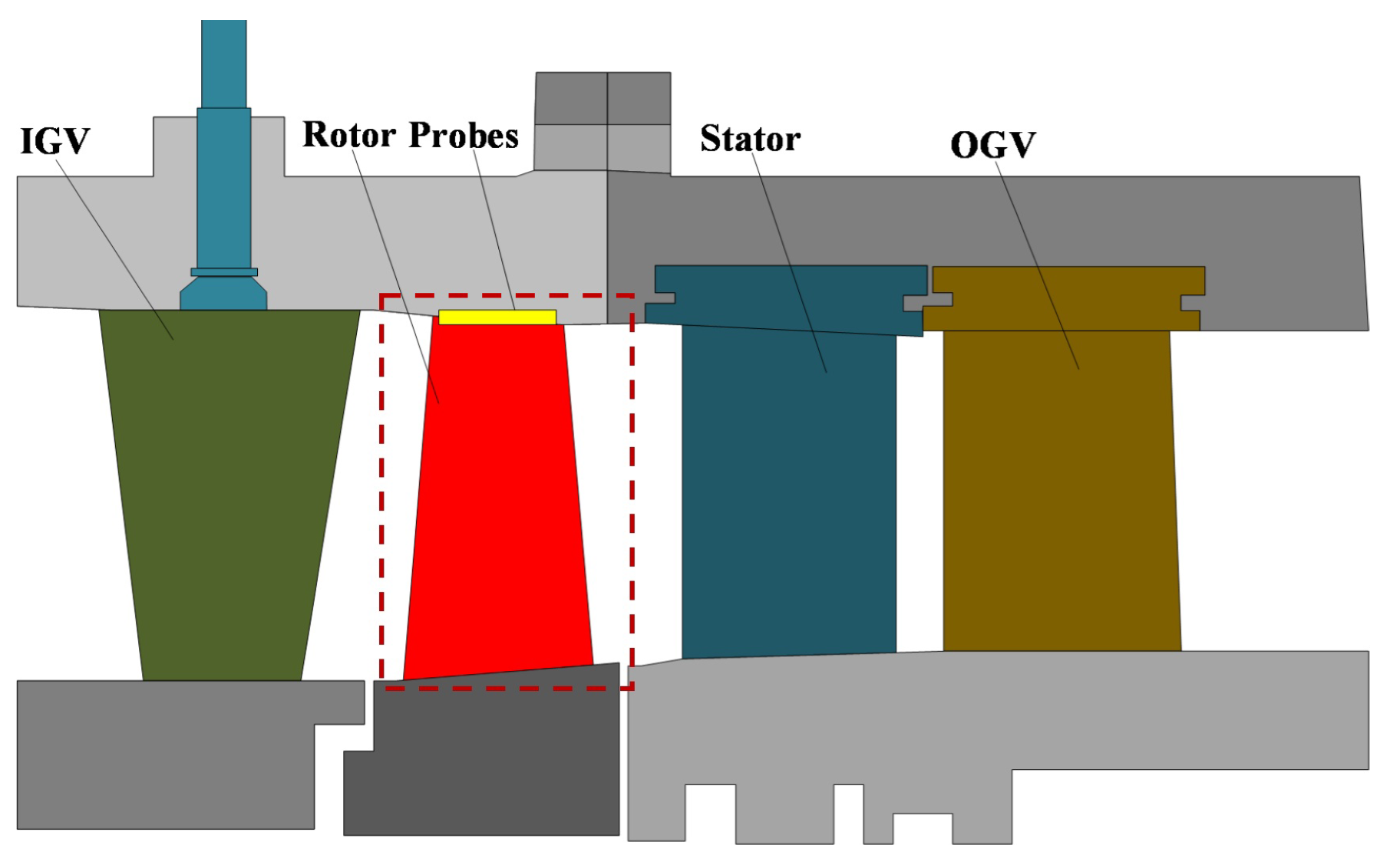
The compressor investigated in the present study is an in-house 1.5-stage transonic axial compressor with 22 rotor blades and a tip clearance of 0.82% chord length, which is modeled from the first stage of an F-class gas turbine. Its schematic structure and design parameters are shown in Figure 1 and Table 1, respectively.
2.2. Mesh for DES Calculation
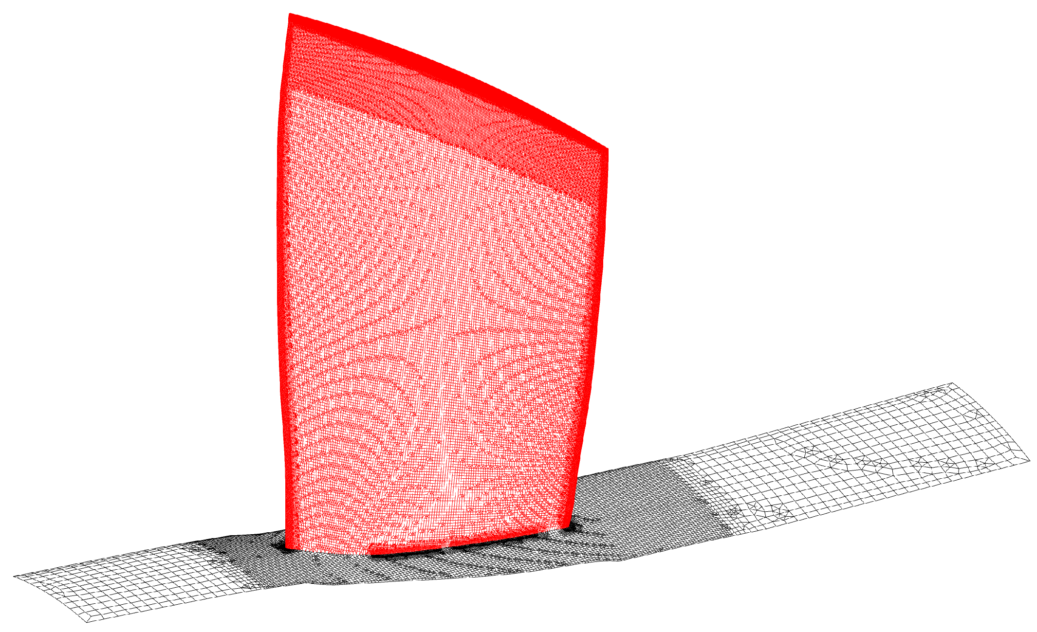
The computational domain is the rotor part (indicated by red dashed line in Figure 1) with inlet and outlet boundaries extended for one-axial chord and two-axial chord, respectively. An unstructured hex-dominant mesh is employed in the DES calculation. As shown in Figure 2, a relatively coarse grid with a refined tip region is adopted to make a trade-off between the flow field resolution and the calculating resources required. To capture the detailed structure of the TLV, the local grid scale at the tip region needs to be at least an order of magnitude smaller than the tip clearance scale in three dimensions, which would be a great challenge if we use a conventional structured mesh. The final mesh is an hybrid grid containing hexahedrons, tetrahedrons, and prisms, with a total element number of 12.3 million, 10 nodes applied in boundary layers to ensure and 27 nodes applied in the tip clearance region with .
2.3. Solver Theory and Calculation Settings
A commercial solver package, FLUENT (14.0, ANSYS, Inc., Canonsburg, PA, USA), was used in the present work, which is a three-dimensional, time-accurate code with implicit second-order scheme, long applied to the field of axial compressors and tip leakage flow [31,32,33,34,35,36,37]. The compressible forms of the Reynolds-averaged Navier–Stokes equations were solved in the fluid domain with gravity and volumetric heat source neglected:
where is the viscous stress tensor, is the Reynolds stress tensor, and is the turbulent thermal conductivity.
The ideal air was chosen as the fluid material, which follows the equation of state:
The properties of air are: molecular weight M = 28.966 g/mol, specific heat capacity at the constant pressure = 1004.4 kJ/(kg · K), thermal conductivity = 0.0261 W/(m · K), and dynamic viscosity is determined by the Sutherland’s formula [38].
The constitutive equations of Newtonian fluid were adopted to model the viscous stress term:
where is the deformation rate tensor. The Reynolds stress term was modeled using the Boussinesq hypothesis, as follows:
For the detached-eddy simulation, the DES97 model, first developed by Spalart et al. [39], was adopted in the present study with a default DES coefficient of 0.65 [40]. In the DES97 model, the near-wall distance d in the original S-A turbulence model [41] has been replaced by the DES length scale , as shown in Equation (7):
where is the working viscosity and is the kinematic viscosity. is a function of another scalar which can be chosen from the vorticity magnitude or the deformation rate [41]. , , , and are coefficients of the S-A turbulence model, whose definitions can all be found in [41]. The DES length scale is defined as follows:
where is the local grid scale and is a coefficient in this model. According to Equation (8), DES length scale will recover to the near-wall distance d when . This always happens inside a boundary layer so that the original S-A turbulence model is activated. Nevertheless, in the mainstream with high Reynolds number, the production term will balance with the destruction term [39] so that Equation (7) becomes:
If is defined as the deformation rate and we choose properly, Equation (9) can be the Smagorinsky-Lilly model [42] for LES:
where is the deformation rate. It is worth noting that the RANS equation and the LES equation are formally identical at some time. Taking Equation (2) for example, once a suitable turbulence model is introduced into the momentum equations, the equation itself will no longer carry any information concerning their derivation (averaging). This is true if we always adopt eddy viscosity models in RANS or LES. The tensor can be the Reynolds stress for RANS when we consider the superscript “” as “time-averaging”. Whereas, can also be the sub-grid-scale stress for LES when the superscript was treated as “spatial-filtering”. In general, the DES length scale acts as a switch for RANS and LES. Therefore, the DES97 model can use LES method in the mainstream and activating RANS method (with S-A turbulence model) inside the boundary layer.
We conduct DES calculations at three working conditions, namely near choke point (NC), peak efficiency point (PE) and near stall point (NS), as shown in Table 2. The physical time of each time step is s, which is small enough to include at least 110 time steps in one blade passing period. Mass flow rate and static pressure were monitored during the calculation to ensure a good convergence. Pressure monitors are located on the tip region of the rotor, with eight points on the casing and one on the blade tip, as shown in Figure 3. As for boundary conditions, adiabatic nonslip-wall conditions were adopted for all solid walls. Radial distributions of total pressure, total temperature, and flow angles were given at the inlet using UDF (user-defined function) files. Static pressure distribution was specified at the outlet.
2.4. Grid Independence Study
The grid independence study was based on RANS calculations with 7 sets of grids at PE, shown in Table 3. The current mesh for DES is the NO.7 grid, which is confirmed to be grid-independent according to Figure 4. We may conclude that the current mesh for DES can provide us a grid-independent result in RANS region. However, the LES region is naturally grid-dependent because the cut-off scale is related to local grid scale. A finer mesh always means a better resolution of the flow field. So an appropriate mesh for LES should meet the requirements of , which has already been checked in Section 2.2.
3. DES Results
3.1. Validation
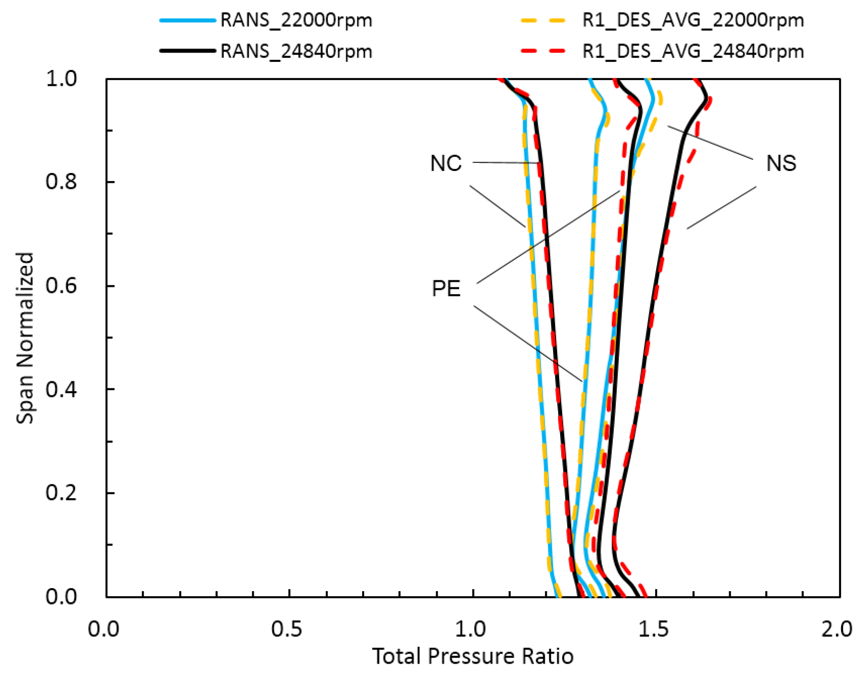
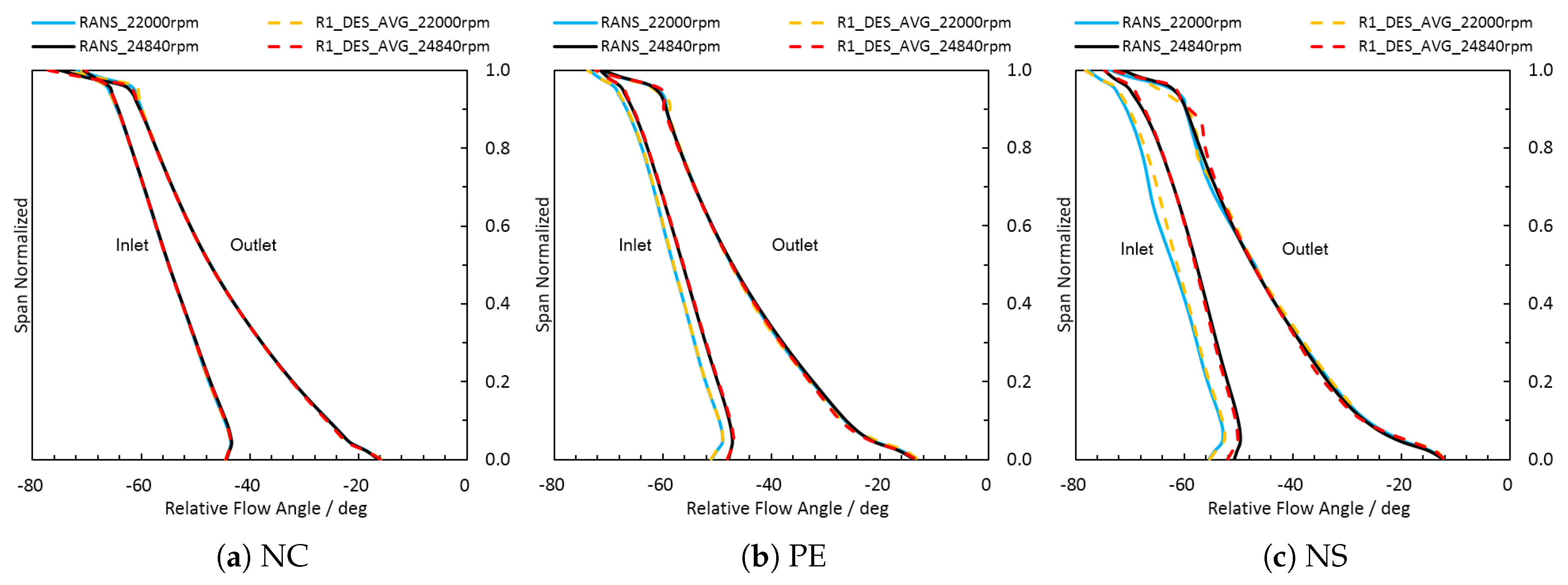
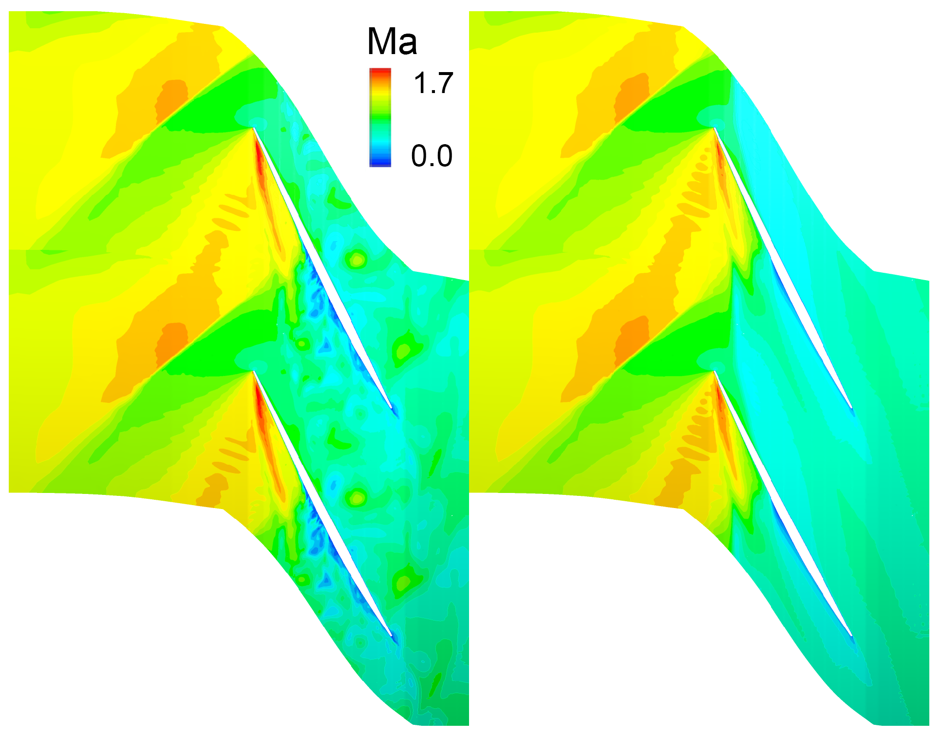
DES results are compared with the experimental data as well as multistage RANS results to ensure a reasonable prediction of the overall flow field, as shown in Figure 5. Please note that the point NS1 and point NS2 were both at near stall conditions. These two points were at same working conditions except for the outlet static pressure. We slightly raised the static pressure (1kPa on average) at the outlet boundary for NS1 then we got NS2, aimed at further approaching the stall limit. Numerical calculations have a good prediction for the performance trend of the compressor at different rotating speeds, especially for the total pressure ratio. As for DES results, the maximum deviations of averaged mass flow rate and total pressure ratio at three working conditions are 0.25% and 0.94%, respectively. Other flow details were compared with corresponding RANS results. Figure 6 and Figure 7 shows radial distributions of total pressure ratio and relative flow angle. Parameter distributions of the DES results were consistent with RANS results, indicating the predictions of averaged flow field are not worse than those of RANS. In addition, Figure 8 shows the comparison of relative Mach contour at 99.3% span (slightly below the blade tip) at near stall point at design speed. These two results near the top region have no conflicts in the shock location or the leakage flow behavior, indicating tip leakage flow was correctly captured in DES calculations. In general, DES results are relatively reliable in the present simulation and can be used for following analysis of the tip leakage flow. Besides, there is no experimental data at the design speed. So we conducted the DES calculation at 22,000 rpm instead and compared it to the experimental data aiming to validate the numerical method.
Moreover, the correct switch of LES and RANS is critical in DES calculations and needs to be checked in the present study to reduce the impact of grid-induced separation(GIS) and grey area problems of the model itself. A criterion to distinguish LES region from RANS region is as follows:
where indicates LES method is switched on and for RANS. Figure 9 shows LES and RANS regions in DES calculations at 90% span, with LES switched on in the mainstream and RANS used inside the boundary layer as expected. Other locations such as 10%, 50% spans and axial cuts were also checked at different working conditions. The switch is appropriate, and no considerable separation was found in the flow field, which contributes to the credibility of present calculations.
3.2. Unsteadiness at NS Point
The tip leakage flow in high-speed compressors has self-induced unsteadiness features [4,43]. In present calculation, by monitoring nine static pressure points, it is found that the fluctuations at NS point is much stronger than PE point and NC point. Therefore, the following part will mainly focus on the unsteadiness at NS condition.
Figure 10 shows the static pressure convergence history of different monitoring points. Point 1, 2 and 5 experienced weaker pressure fluctuation than the rest. It is worth noting that point 1 and 2 are exactly in the initial trajectory of the TLV and in front of the shock near suction side, while point 5 is at the leading edge and after the bow shock. For transonic rotors, it is typical that the TLV starts from the leading edge of tip blade, traveling towards the adjacent pressure side. It passes through and interacts with the bow shock, then imprints on the adjacent pressure side, and finally develops downstream along the blade surface. In other words, these three points mentioned above are far away from the interaction region of TLV and the shock, indicating that neither the TLV nor the shock alone is the root cause of the unsteadiness. In addition, points 6 to 9, which experienced strong fluctuations in static pressure, are also located along the trajectory of TLV. However, what makes a difference is that these points are all located after the shock wave. From this aspect, it is exactly the interaction between TLV and the shock that leads to the unsteadiness of the tip region. The detailed reasons will be explained in next section.
Figure 11 shows the spectrum of some representative monitor points at near stall point, which is the result of the fast Fourier transform of the time series data. The frequency characteristics of each point are not the same. Wide though the frequency bands are, they do share some similarities, that is, peak values appeared near two specific frequencies 0.64 BPF and 1.80 BPF. It is worth noting that the former is close to the characteristic frequency of tip leakage flow in typical transonic compressors, for instance, 0.6 BPF [44] for NASA Rotor 37 and 0.57 BPF [4,20] for Darmstadt Rotor 1. Other monitoring points with large fluctuation, such as point 8 and point 9, have similar results as well.
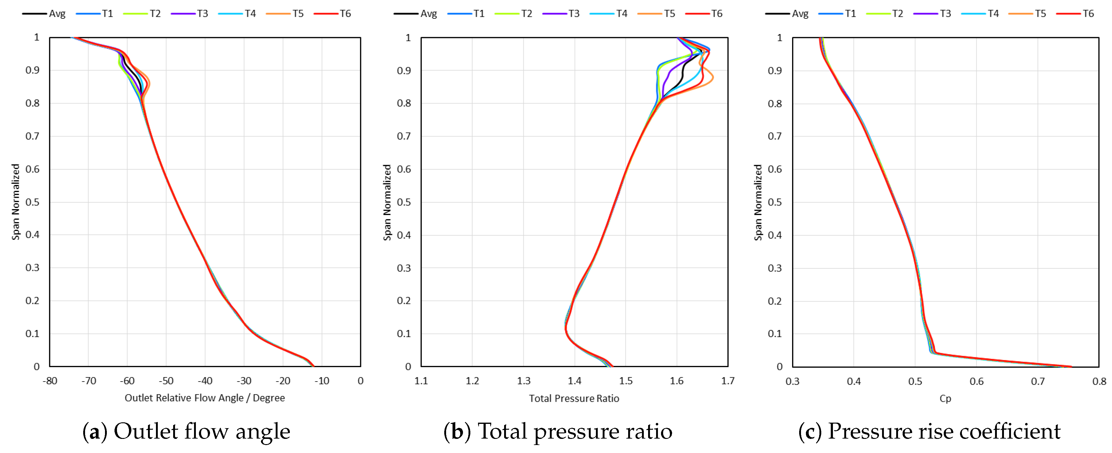
The unsteadiness near the tip region inevitably affected the performance of the compressor and is the critical reason for the fluctuation in overall parameters at near stall point, as shown in Figure 12. T1 to T6 are six different moments with the same time interval s, whose corresponding frequency is about 2.2 BPF. Obvious unsteady feature exists above 80% span with a fluctuation range of about 10 degrees for the outlet flow angle and 0.1 (about 6.5% of the time-averaged total pressure ratio) for the total pressure ratio, while the unsteadiness is weak in the middle and root span, indicating that tip leakage flow is an essential factor causing instability at NS point. Nevertheless, there is no obvious fluctuation of the static pressure rise coefficient among the whole blade height range, which means the unsteadiness of the top flow field is mainly caused by the fluctuation of kinetic energy and can be a proof for the wake-like nature of the TLV when passing through the shock [45].
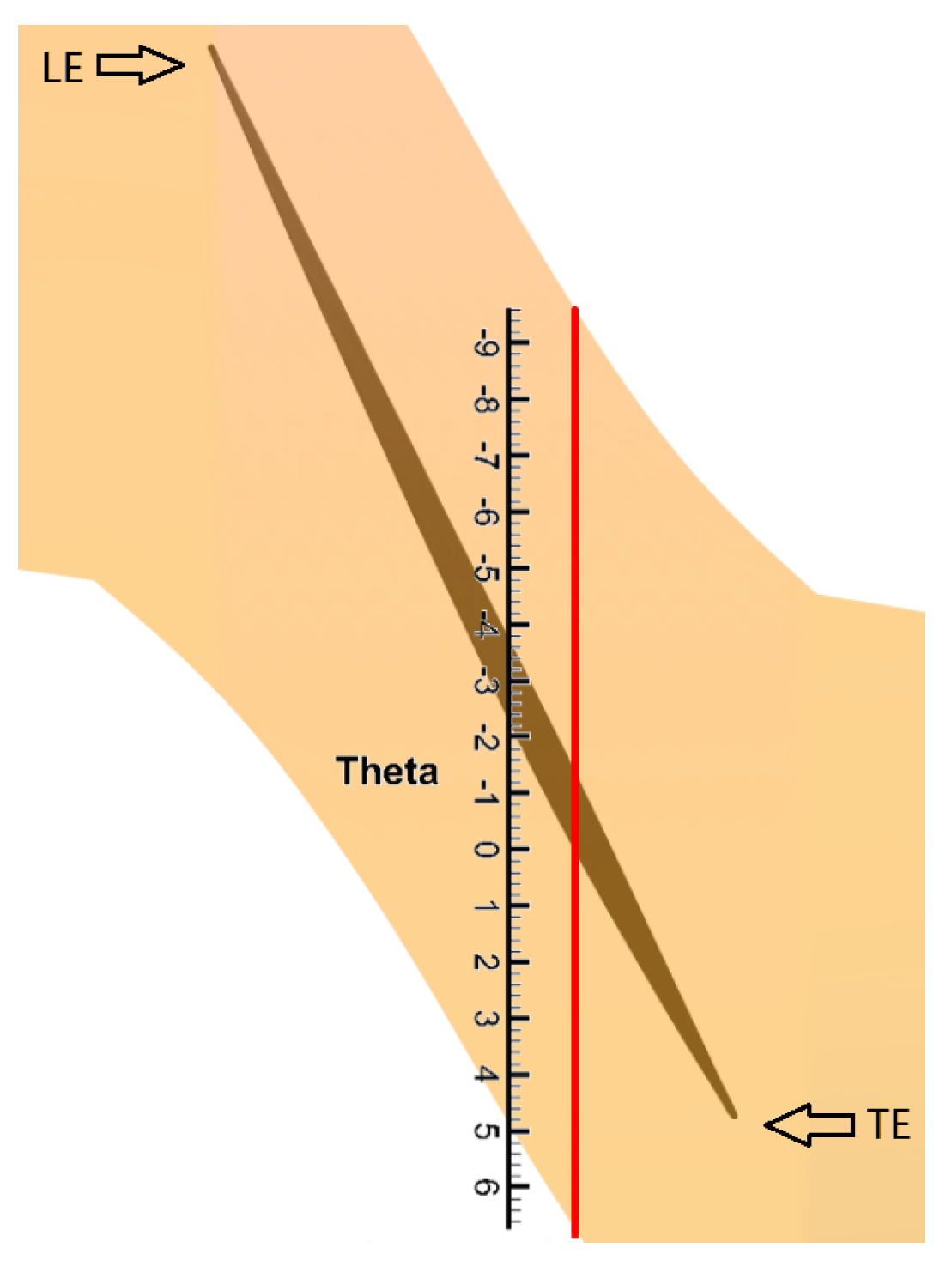
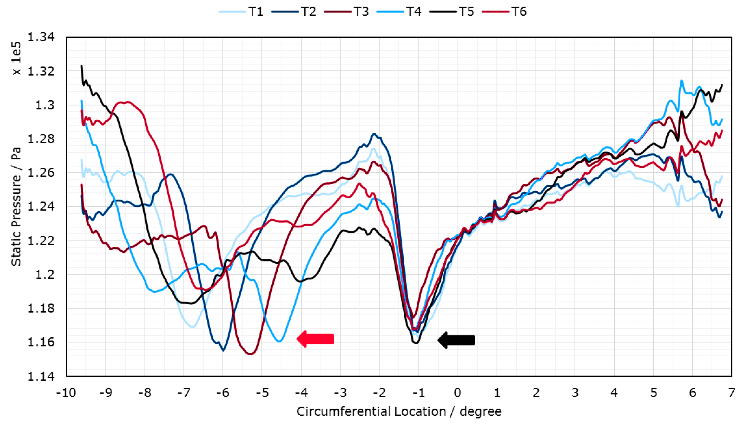
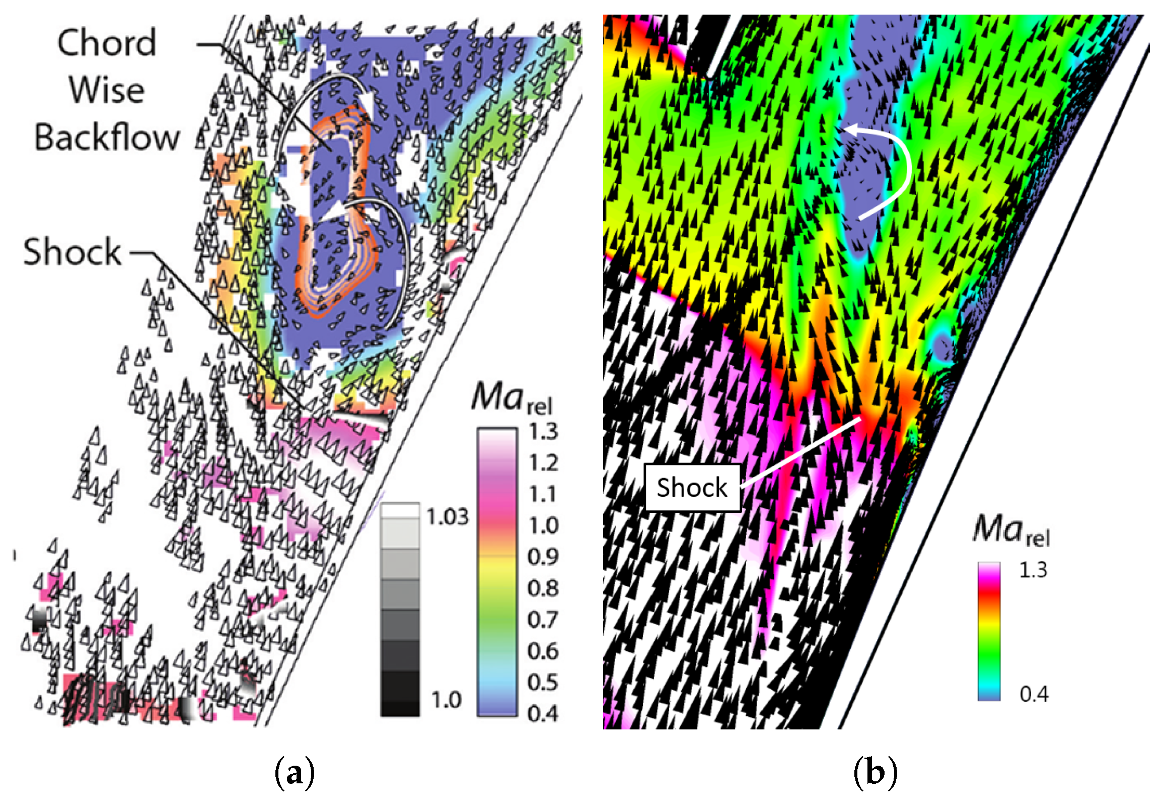
Figure 13 is the top view of R1 shroud with blade profile imprinted. We chose a certain axial location (red line) and obtained its circumferential distribution of static pressure in one period, as shown in Figure 14, taking circumferential angle as the abscissa. There are two low pressure regions, one is at about −1 degrees (indicated by the black arrow) and the other is from −4.5 to −7 degrees (indicated by the red arrow). The former region is at the tip clearance region, very little influenced by the unsteadiness, while the latter experienced a strong oscillation at different time steps, with the valley traveling from the left side to the right side then returning to the left side. According to Figure 13, the latter region is near the pressure side of the tip blade, exactly located in the TLV trajectory after the shock, on its way to hit the adjacent pressure side and to develop downstream. The oscillation of pressure valley indicated that the TLV was no longer stable at NS point and was oscillating in the blade passage.
Figure 15 can illustrate the above phenomena more clearly, with black dash-dotted line indicated the same axial location in Figure 13. Interacted with the shock and the parallel small vortex, TLV started to swing tangentially at a distance after the shock. This resulted in a small oscillation, developing downstream with an increasing amplitude. As is known, TLV has a lower static pressure value and a lower axial velocity than the mainstream. Every time the trajectory of TLV swept over a certain point, that location would experience a drop in static pressure as well as axial velocity, which is the cause of the oscillation in Figure 14. Eventually, it caused the oscillation of overall parameters such as outlet flow angle, pressure ratio, or efficiency.
In general, the unsteadiness of the rotor at NS point is mainly manifested at the tip region, closely related to the TLV. The unsteady characteristics in middle span or root span can be totally ignored in comparison. Neither the TLV nor the shock alone is the origin of the unsteadiness. It was found that the TLV became unstable after the interaction with the shock and experienced a stronger oscillation when developing downstream. The most unstable region in this transonic rotor is near the pressure side of the tip blade, which is similar to the conclusions [4] for Darmstadt Rotor 1.
3.3. Detailed Structure of Tip Leakage Flow
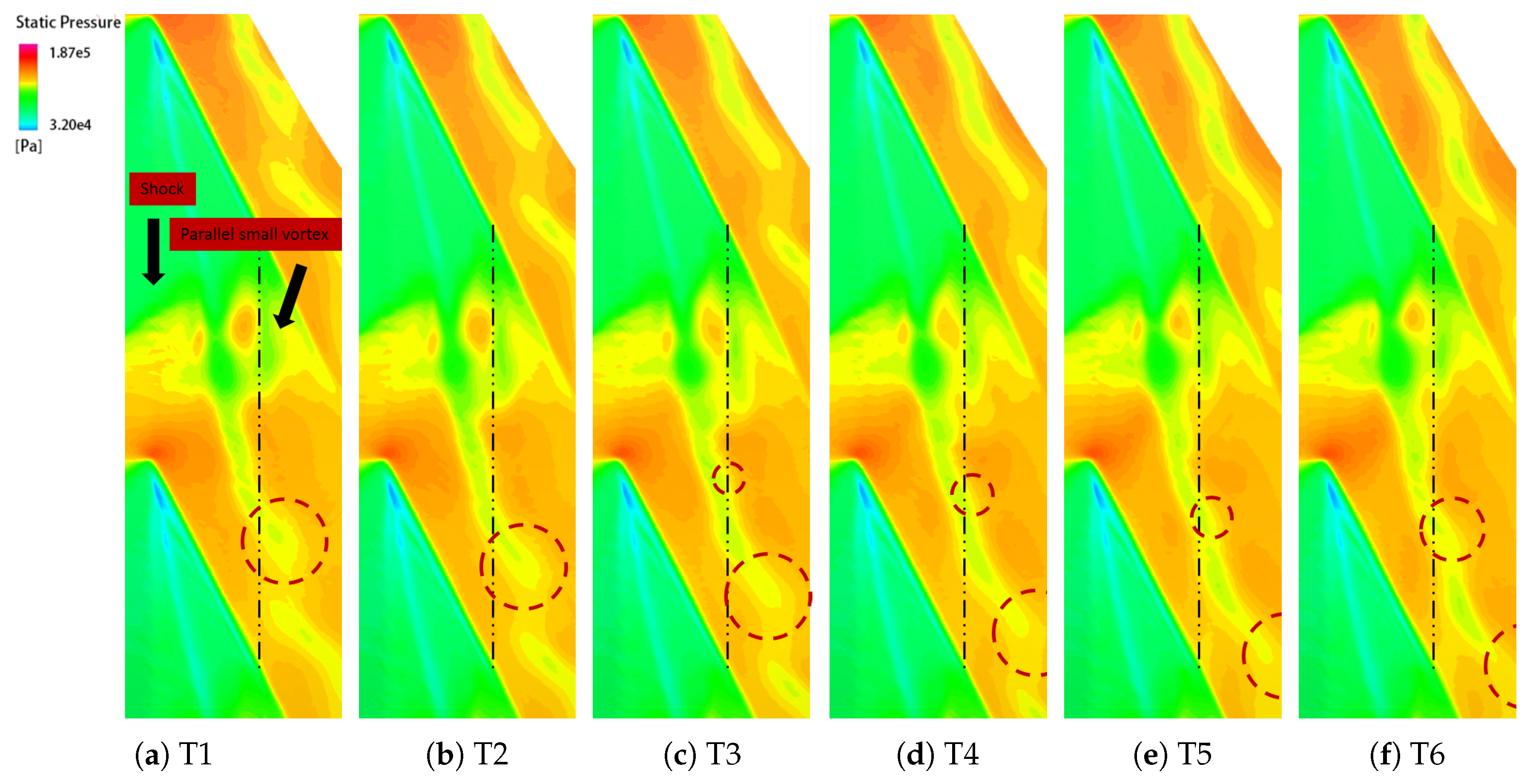
DES calculation can obtain detailed information of the top flow field than RANS and may provide some clues for the unsteady characteristic mentioned above. The general structure of tip leakage flow can be clearly observed in Figure 16, with shock position indicated by dashed line. The vortex structures are in three different forms as the operating condition changes.
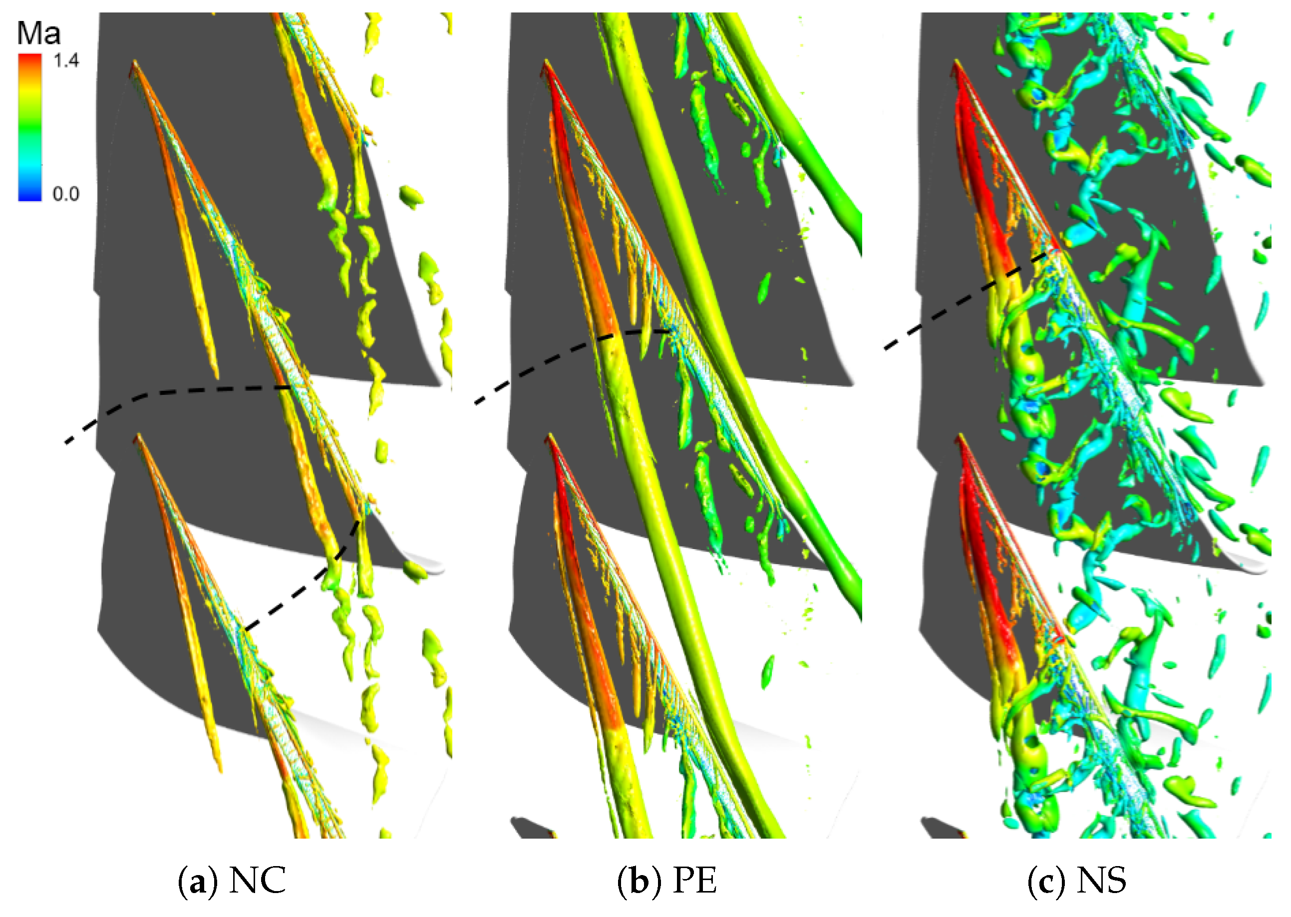
At the NC point, there are two shocks, one is the bow shock near the leading edge and the other is the passage shock near the trailing edge. Under this condition, the pressure gradient in the tip clearance is relatively small and the TLV started from the leading edge is weak as well. As a result, the vortex core was slenderer in Figure 16a and vanished directly after the bow shock. Meanwhile, the TLV was too weak to draw downstream leakage fluid into, which led to another vortex system after the middle chord of the blade. At PE point, however, the blade load increased and the leading-edge TLV became stronger, so that most leakage fluid can be drawn into the main leakage vortex. The characteristics of the TLV were kept so well in the developing process that the vortex core remained continuous when passing through the shock with a slight expansion in volume, which indicates a stable flow state at PE point. At NS point, the entire top flow field had a very rich flow pattern, and there were many small vortex structures after the shock. Some of the small vortices were developed from the main leakage vortex. The other parts were from the secondary leakage, that is, after imprinting the pressure surface of the adjacent blade, the TLV leaked to the next blade passage again through the tip clearance of the adjacent blade.
The complex flow field at top region is consistent with the strong unsteadiness mentioned above at NS point. The static pressure oscillation in Figure 15 was caused by the “shedding” of small vortices after the shock. The small vortices did not exist at NC point or PE point and mainly came from the main leakage vortex, which is probably caused by the interaction with the shock. When passing though the bow shock, the TLV at NS point changed from a single solid core to many separate vortices.
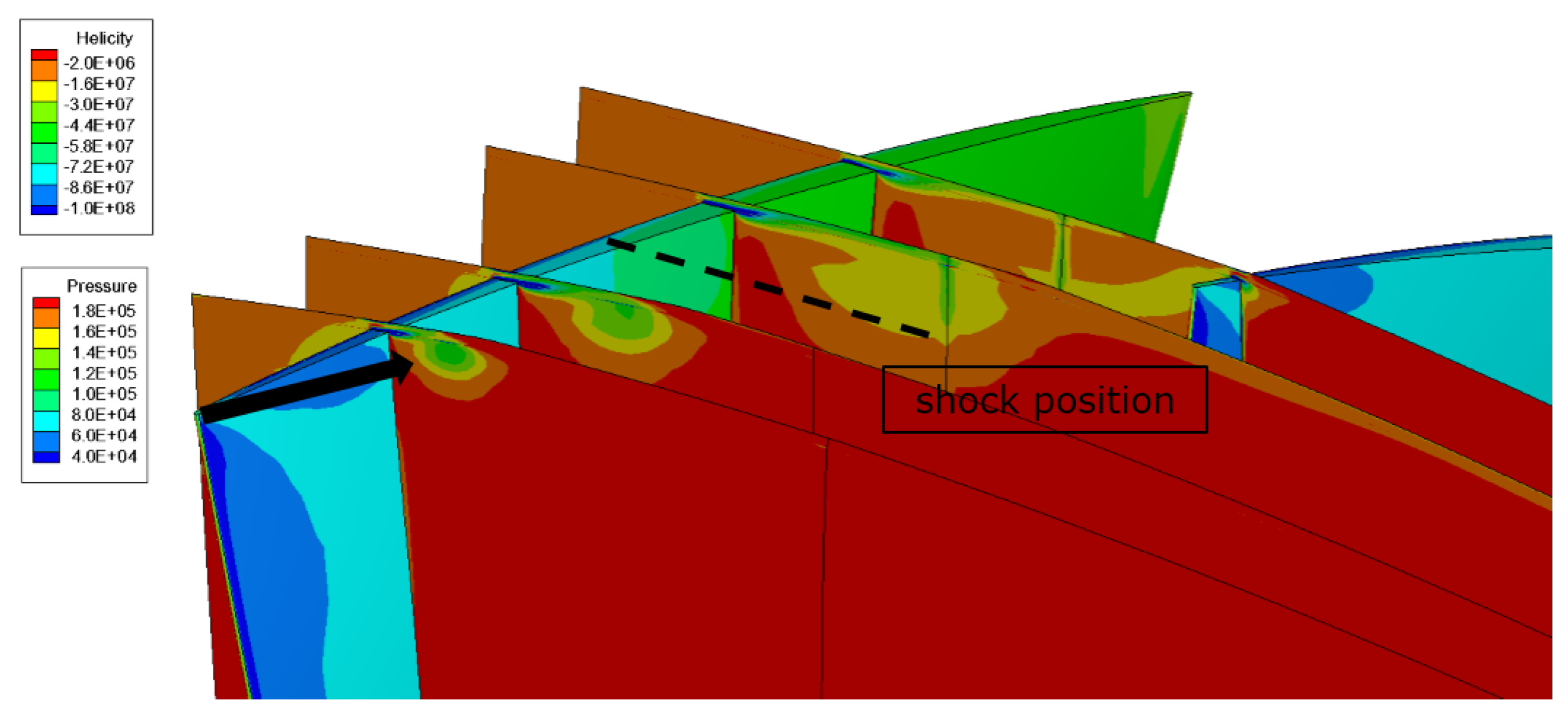
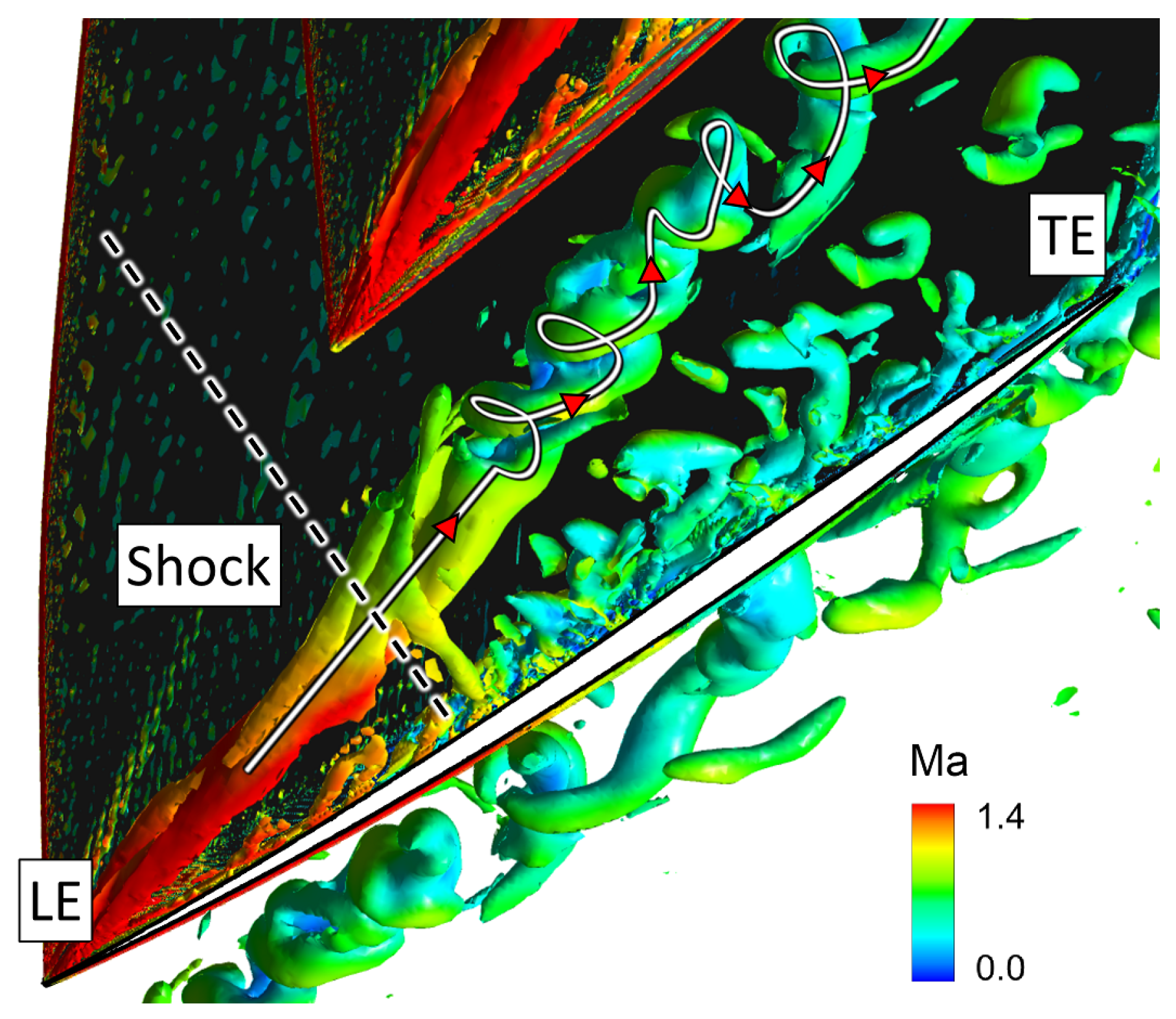
Figure 17 is the helicity distribution of different crossflow planes at near stall point, which is used to characterize the intertwining degree of the fluid around TLV core, with the blade surface colored by static pressure, the shock position indicated by the black dotted line, and the beginning of the TLV indicated by the black arrow. The vortex core before the shock was concentrated and slowly increasing in volume. After the shock, the helicity distribution was dispersed and not concentrated anymore, which indicated that the fluid no longer moved around the vortex core tightly after the shock. The distance between the four crossflow planes can be approximated as isometric, but the helicity distribution before and after the shock surface is quite different, which means that the vortex core experienced an abrupt change in its internal structure. Combined with the vortex structure in Figure 16c, we can conclude that a vortex breakdown took place after the interaction between TLV and the shock.
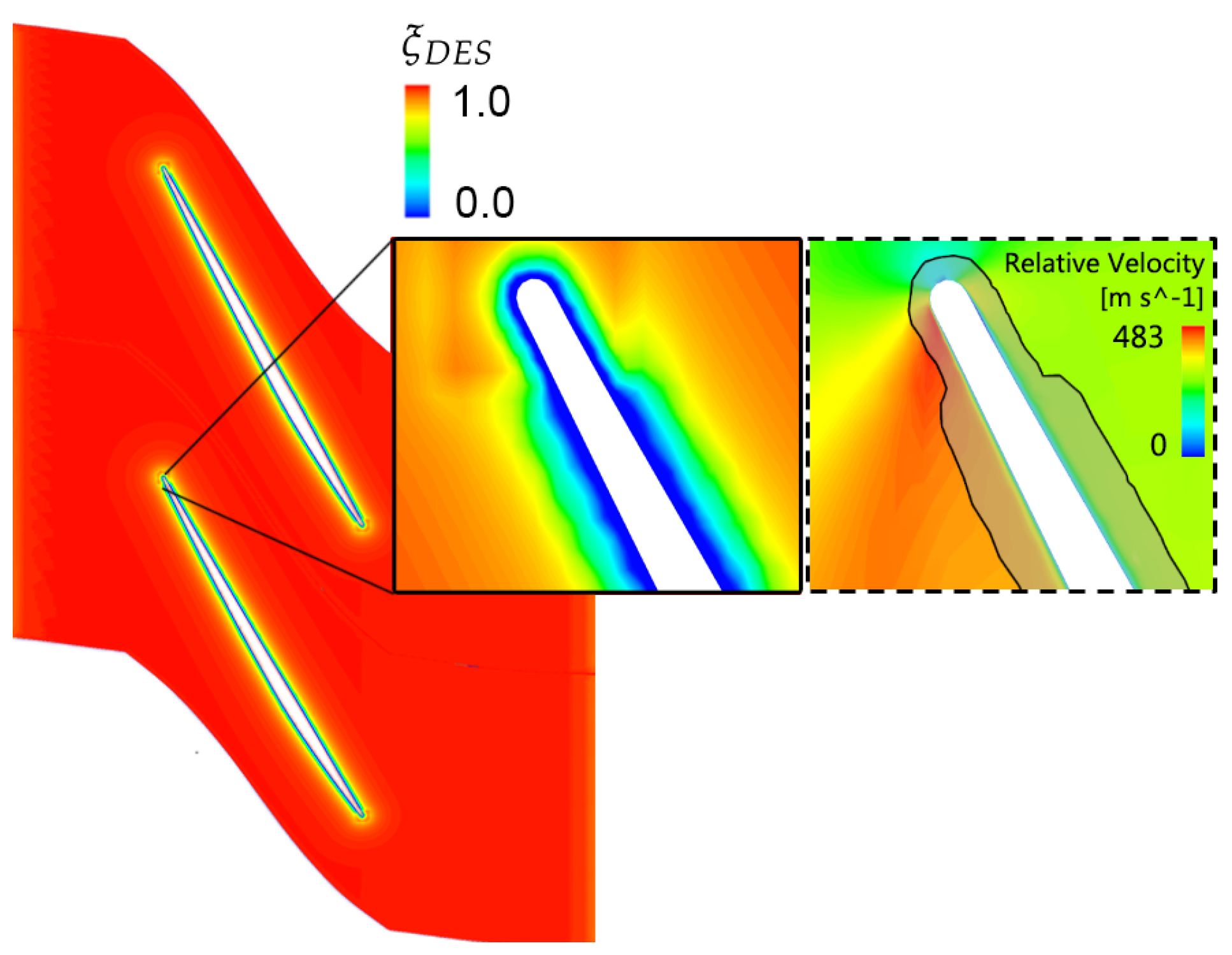
The breakdown process can be clearly illustrated in Figure 18, which is a transient isosurface colored by relative Mach number. It is confirmed that the TLV changed to a three-dimensional structure and was not axisymmetric anymore when passing through the shock. The vortex core changed its direction to a perpendicular path and started to rotate around the original one when developing downstream, which is the typical structure of a spiral-type breakdown. The structure after the onset of the breakdown process is not stable, with rotating phase related to the flow time, thus causing strong unsteadiness. This contributes a lot to our understanding of the oscillation after the shock in Figure 15 that the previous view on the unsteady flow behavior of the leakage vortex may be incomplete. The unsteadiness is not a two-dimensional phenomenon inside the S1 plane, but a three-dimensional structure in nature. The underlying reason behind is the spiral-type vortex breakdown after the interaction with the shock.
To the author’s knowledge, this is probably the first time that a detailed structure of the breakdown process for the TLV in a transonic compressor is obtained in numerical investigations. In addition, PIV (particle image velocimetry) measurements of another transonic compressor near stability limit were conducted [46], whose results are in great agreement with the present calculation results, as shown in Figure 19.
4. Discussion
Vortex breakdown is a very complex flow phenomenon and is an independent branch in fluid mechanics. The interaction of a streamwise vortex and a normal or oblique shock under supersonic conditions could lead to a vortex breakdown phenomenon. The interacting process and mechanisms were widely studied [47,48,49,50]. Recently, lots of efforts [51,52,53,54,55] have been made extending the state of knowledge regarding onset, internal structure and mode selection of vortex breakdown. In the present study, a shock-induced spiral-type vortex breakdown was found at NS. We will deal with the related structure of the breakdown process in this section.
In transonic compressors, the shock wave in the rotor passage can provide a large adverse pressure gradient, with a great influence on the streamwise velocity in the vortex core. As shown in Figure 20, subfigure (a) is the isosurface, which illustrates the breakdown process. Subfigure (b) is streamwise velocity contour at the same viewpoint, which indicates the component of relative velocity in the vortex trajectory direction, and subfigure (c) demonstrates the surface streamline. The corresponding cut plane is represented by the red point line in the top view and the location of the bow shock near the suction surface is characterized by the black dashed line. The vortex breakdown is clearly observed in the upper figure with its initial location indicated by the red circle. The breakdown location was not at the shock surface exactly, but at a certain distance downstream, which is in qualitative agreement with experimental results in Figure 19a. Leibovich [56] pointed out that this axial interval is several vortex-core diameters in length. It is worth noting that the initial location of vortex breakdown in (a) coincided with the location S1 in (b) where the streamwise velocity of the vortex core was zero, which indicates that the breakdown of the leakage vortex is closely related to the stagnation point in the center of vortex core. Please note that there were not only one stagnation point in (b). Along with subfigure (c), we could observe a recirculation zone between the two stagnation points S1 and S2. This is consistent with the direct numerical simulation of vortex breakdown in swirling jets and wakes by Ruith et al. [52].
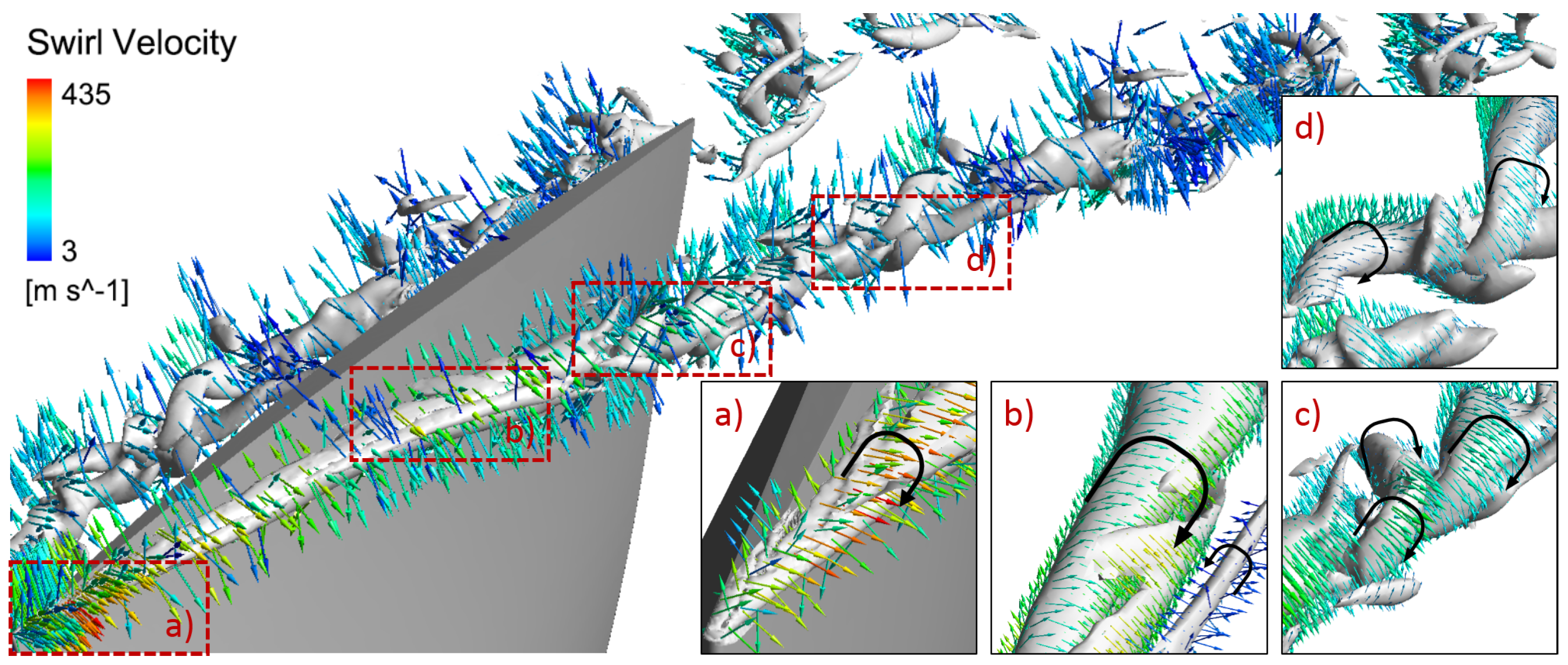
Figure 21 is the swirl velocity vector of the TLV, demonstrating the rotating direction of the TLV before and after the breakdown. For clarity, the adjacent blade was hidden, and the larger images of the dashed zones might have a different view point. Whether before or after the breakdown point, the vortices were temporally rotating in the same direction as the initial TLV, except for the induced vortex in (b). However, the helices after breakdown were coiling in the opposite direction (more clear in Figure 18). This is similar to the findings of Pasche et al. [57] who conducted experiments on obstacle-induced spiral vortex breakdown. The breakdown helices originating at a locally wake-like profile have negative winding sense [52]. Of course, the TLV had a wake-like profile in nature and the breakdown structure in the present study contributed to this view.
The causes of vortex breakdown are very complicated. The generation of the recirculation bubble of the vortex breakdown remains unclear but the spiraling motion of the flow behind the recirculation bubble comes from a global unstable mode of the flow [53]. The same mechanism is also observed without recirculation bubble [57], the spontaneous spiraling motion is due to a self-sustained instability. At present, it is consistent to conclude that the reverse pressure gradient and the strength of the vortex itself are crucial factors in the vortex breakdown process [48]. The adverse pressure gradient characterizes the deceleration of the vortex core along the streamwise direction. Criteria for vortex breakdown based on the interaction between the Rankine vortex and the normal shock waves were proposed by Mahesh [58], Smart and Kalkhoran [49] and other scholars. As shown in Figure 22, the abscissa is the freestream Mach number, reflecting adverse pressure gradient in the streamwise direction. The ordinate is the swirl ratio before the shock, which reflects the intensity of the vortex. The swirl ratio is defined as follows:
where is the maximum swirl velocity component and is the streamwise velocity component in the vortex core.
The interaction between the TLV and the bow shock in the transonic compressor could be simplified to the interaction of normal shock and vortex. Both the compressor in the present paper (red marks) and Rotor 37 (blue marks, [44]) exceeded the breakdown limit at NS conditions, and the breakdown of leakage vortex did occur in the detailed flow field. In addition, at PE point and NC point, the vortex breakdown phenomenon was not observed in the present calculation, which is still in good agreement with the breakdown criterion. As the operating point moves to the NS point, the swirl ratio will increase sharply with the increase of the leakage vortex intensity, while the change of Mach number in the axial direction of the vortex core is not obvious. Therefore, transonic rotors with heavy blade loading are likely to experience leakage vortex breakdown at NS point.
We could use the mechanism for the shock-induced breakdown to illustrate the interacting process between the TLV and the bow shock or the breakdown process of the TLV in transonic compressors. When the vortex passes through the shock, the streamwise velocity decreases rapidly due to the strong adverse pressure gradient produced by the shock. The swirl component, however, is orthogonal to the shock surface and is not much affected. In other words, the attenuation of the streamwise component is far greater than that of the swirl component [48]. When the shock is strong enough, the streamwise velocity will decay to zero after the interaction. Under this circumstance, the breakdown phenomenon of the TLV is likely to occur.
The small vortices produced by the TLV vortex breakdown are distributed in the tip region, causing a large blockage effect in the rotor passage. The low energy fluid might subsequently result in leading-edge spillage or induce a spike-type stall inception. Therefore, how to postpone or eliminate the breakdown of TLV may become one of the important ways to enhance the stability at NS point and enlarge the surge margin of transonic compressors.
5. Conclusions
In this paper, a numerical investigation of a transonic compressor rotor using DES method is conducted at three working conditions, focused on the structure of tip leakage flow, the interaction with shock wave and the unsteady characteristics.
Strong unsteadiness was found at NS point with the characteristic frequencies of 0.64 BPF and 1.80 BPF. The most unstable region for this transonic rotor is in the rotor passage near the pressure side of the tip blade, which is the result of the interaction between the TLV and the shock. The affected area is mainly located at the tip region, causing a considerable fluctuation in total pressure distribution and flow angle distribution above 80% span. The unsteadiness at NC point and PE point is not obvious.
Detailed structures of the tip leakage flow were captured, closely related to the working condition. At the NS point, a vortex breakdown can be observed downstream the bow shock. While, at NC point or PE point, the TLV breakdown did not take place. The breakdown process at NS point was confirmed in a spiral-type form. The vortex core changed its direction to a perpendicular path and started to rotate around the original one when developing downstream. Whether before or after the breakdown point, the vortices were temporally rotating in the same direction as the initial leakage vortex. Whereas, the helices after breakdown were coiling in the opposite direction. The breakdown of the TLV generated unstable small vortices and contributed greatly to the unsteadiness at NS point.
Author Contributions
X.S. acquired the numerical data and wrote the paper; and X.R., X.L. and C.G. revised the paper and offered useful suggestions to write the paper.
Funding
This paper is supported by National Science and Technology Major Project (No: 2017-II-0007), National Natural Science Foundation of China (No. 51806118) and by a grant from the Science & Technology on Reliability & Environmental Engineering Laboratory (No. 6142A0501020317).
Acknowledgments
The author thanks Senior Engineer JianBai Li for his critical comments and helpful advice. This work is supported by the “Explorer 100” HPC Platform, State Laboratory for Information Science and Technology, Tsinghua University.
Conflicts of Interest
The authors declare no conflict of interest.
Nomenclature
| the coefficient in DES97 model | |
| specific heat capacity at the constant pressure | |
| the coefficient in Smagorinsky-Lilly model | |
| DES length scale | |
| e | inner energy |
| E | total energy, |
| H | total enthalpy, |
| k | turbulent kinetic energy |
| M | molecular weight |
| Mach number | |
| p | pressure |
| gas constant, | |
| S | deformation rate, |
| deformation rate tensor | |
| T | temperature |
| u | velocity |
| x | Cartesian coordinates |
| nondimensional wall distance | |
| local grid scale | |
| nondimensional grid scale in x direction | |
| nondimensional grid scale in y direction | |
| nondimensional grid scale in z direction | |
| thermal conductivity | |
| turbulent thermal conductivity | |
| dynamic viscosity | |
| turbulent eddy viscosity | |
| kinematic viscosity | |
| the working viscosity in S-A model | |
| sub-grid-scale kinematic viscosity | |
| turbulent kinematic viscosity | |
| a criterion to distinguish LES region from RANS region | |
| density | |
| viscous stress tensor | |
| Reynolds stress tensor or sub-grid-scale stress tensor |
Abbreviations
| BPF | Blade passing frequency, (Hz), where n is the rotation speed of the axis with the unit rpm |
| DES | Detached-eddy simulation |
| LES | Large eddy simulation |
| NB | Number of rotor blades |
| NC | Near choke point |
| NS | Near stall point |
| PE | Peak efficiency point |
| PIV | Particle image velocimetry |
| RANS | Reynolds-averaged Navier–Stokes |
| SGS | sub-grid-scale stress |
| TLV | Tip leakage vortex |
| UDF | User-defined function |
References
- Storer, J.A.; Cumpsty, N.A. Tip leakage flow in axial compressors. J. Turbomach. 1991, 113, 252. [Google Scholar] [CrossRef]
- Gerolymos, G.A.; Vallet, I. Tip-clearance and secondary flows in a transonic compressor rotor. J. Turbomach. 1999, 121, 751. [Google Scholar] [CrossRef]
- Tan, C.; Day, I.; Morris, S.; Wadia, A. Spike-type compressor stall inception, detection, and control. Ann. Rev. Fluid Mech. 2010, 42, 275–300. [Google Scholar] [CrossRef]
- Du, J.; Lin, F.; Chen, J.; Nie, C.; Biela, C. Flow structures in the tip region for a transonic compressor rotor. J. Turbomach. 2013, 135, 031012. [Google Scholar] [CrossRef]
- Liu, Y.; Tan, L.; Wang, B. A review of tip clearance in propeller, pump and turbine. Energies 2018, 11, 2202. [Google Scholar] [CrossRef]
- Tab, L.; Xie, Z.; Liu, Y.; Hao, Y.; Xu, Y. Influence of T-shape tip clearance on performance of a mixed-flow pump. Proc. Inst. Mech. Eng. Part A J. Power Energy 2018, 232, 386–396. [Google Scholar] [CrossRef]
- Liu, M.; Tan, L.; Cao, S. Cavitation-vortex–turbulence interaction and one-dimensional model prediction of pressure for hydrofoil ALE15 by large eddy simulation. J. Fluids Eng. 2018, 141, 021103. [Google Scholar] [CrossRef]
- Hao, Y.; Tan, L. Symmetrical and unsymmetrical tip clearances on cavitation performance and radial force of a mixed flow pump as turbine at pump mode. Renew. Energy 2018, 127, 368–376. [Google Scholar] [CrossRef]
- Denton, J.D. Loss mechanisms in turbomachines. J. Turbomach. 1993, 115, 621–656. [Google Scholar] [CrossRef]
- Vo, H.D. Role of Tip Clearance Flow on Axial Compressor Stability. Ph.D. Thesis, Massachusetts Institute of Technology, Cambridge, MA, USA, 2001. [Google Scholar]
- Suder, K.L.; Hathaway, M.D.; Thorp, S.A.; Strazisar, A.J.; Bright, M.B. Compressor stability enhancement using discrete tip injection. J. Turbomach. 2001, 123, 14. [Google Scholar] [CrossRef]
- Eveker, K.M.; Gysling, D.L.; Nett, C.N.; Sharma, O.P. Integrated control of rotating stall and surge in high-speed multistage compression systems. J. Turbomach. 1998, 120, 440–445. [Google Scholar] [CrossRef]
- Müller, M.W.; Schiffer, H.P.; Hah, C. Effect of circumferential grooves on the aerodynamic performance of an axial single-stage transonic compressor. In Proceedings of the ASME Turbo Expo 2007: Power for Land, Sea, and Air, Montreal, QC, Canada, 14–17 May 2007; ASME: New York, NY, USA; Volume 6, pp. 115–124. [CrossRef]
- Vo, H.D. Rotating stall suppression in axial Compressors with casing plasma actuation. J. Propuls. Power 2010, 26, 808–818. [Google Scholar] [CrossRef]
- Hoying, D.A.; Tan, C.S.; Vo, H.D.; Greitzer, E.M. Role of blade passage flow structurs in axial compressor rotating stall inception. J. Turbomach. 1999, 121, 735. [Google Scholar] [CrossRef]
- Vo, H.D.; Tan, C.S.; Greitzer, E.M. Criteria for spike initiated rotating stall. In Proceedings of the ASME Turbo Expo 2005: Power for Land, Sea, and Air, Peno, NV, USA, 6–9 June 2005; ASME: New York, NY, USA, 2005; Volume 6, pp. 155–165. [Google Scholar] [CrossRef]
- Deppe, A.; Saathoff, H.; Stark, U. Discussion: “Criteria for spike initiated rotating stall” (Vo, H. D., Tan, C. S., Greitzer, E. M., 2008, ASME J. Turbomach., 130, p. 011023). J. Turbomach. 2008, 130, 015501. [Google Scholar] [CrossRef]
- Yamada, K.; Kikuta, H.; Iwakiri, K.i.; Furukawa, M.; Gunjishima, S. An explanation for flow features of spike-type stall inception in an axial compressor rotor. J. Turbomach. 2012, 135, 021023. [Google Scholar] [CrossRef]
- Hah, C. Effects of double-leakage tip clearance flow on the performance of a compressor stage with a large rotor tip gap. J. Turbomach. 2017, 139, 061006. [Google Scholar] [CrossRef]
- Biela, C.; Müller, M.W.; Schiffer, H.P.; Zscherp, C. Unsteady pressure measurement in a single stage axial transonic compressor near the stability limit. In ASME Turbo Expo 2008: Power for Land, Sea, and Air; American Society of Mechanical Engineers: New York City, NY, USA, 2008; pp. 157–165. [Google Scholar]
- Zhang, Y.; Lu, X.; Chu, W.; Zhu, J. Numerical investigation of the unsteady tip leakage flow and rotating stall inception in a transonic compressor. J. Therm. Sci. 2010, 19, 310–317. [Google Scholar] [CrossRef]
- Hah, C.; Rabe, D.C.; Wadia, A.R. Role of tip-leakage vortices and passage shock in stall inception in a swept transonic compressor rotor. In Proceedings of the ASME Turbo Expo 2004: Power for Land, Sea, and Air, Vienna, Austria, 14–17 June 2004; ASME: New York, NY, USA, 2004; Volume 5, pp. 545–555. [Google Scholar] [CrossRef]
- Hoeger, M.; Fritsch, G.; Bauer, D. Numerical simulation of the shock-tip leakage vortex interaction in a HPC front stage. J. Turbomach. 1999, 121, 456–468. [Google Scholar] [CrossRef]
- Bergner, J.; Kinzel, M.; Schiffer, H.P.; Hah, C. Short length-scale rotating stall inception in a transonic axial compressor: Experimental investigation. In Proceedings of the ASME Turbo Expo 2006: Power for Land, Sea, and Air, Barcelona, Spain, 8–11 May 2006; ASME: New York, NY, USA, 2006; Volume 6, pp. 131–140. [Google Scholar] [CrossRef]
- Iim, H.; Chen, X.Y.; Zha, G. Detached-eddy simulation of rotating stall inception for a full-annulus transonic rotor. J. Propuls. Power 2012, 28, 782–798. [Google Scholar] [CrossRef]
- Spalart, P.R. Detached-eddy simulation. Ann. Rev. Fluid Mech. 2009, 41, 181–202. [Google Scholar] [CrossRef]
- Riéra, W.; Castillon, L.; Marty, J.; Leboeuf, F. Inlet condition effects on the tip clearance flow with zonal detached eddy simulation. J. Turbomach. 2013, 136, 041018. [Google Scholar] [CrossRef]
- Riéra, W.; Marty, J.; Castillon, L.; Deck, S. Zonal detached-eddy simulation applied to the tip-clearance flow in an axial compressor. AIAA J. 2016, 54, 2377–2391. [Google Scholar] [CrossRef]
- Yamada, K.; Furukawa, M.; Tamura, Y.; Saito, S.; Matsuoka, A.; Nakayama, K. Large-scale detached-eddy simulation analysis of stall inception process in a multistage axial flow compressor. J. Turbomach. 2017, 139, 071002. [Google Scholar] [CrossRef]
- Lin, D.; Su, X.; Yuan, X. DDES analysis of the wake vortex related unsteadiness and losses in the environment of a high-pressure turbine stage. J. Turbomach. 2018, 140, 041001. [Google Scholar] [CrossRef]
- Nie, C.; Xu, G.; Cheng, X.; Chen, J. Micro air injection and its unsteady response in a low-speed axial compressor. In Proceedings of the ASME Turbo Expo 2002: Power for Land, Sea, and Air, Amsterdam, The Netherlands, 3–6 June 2002; ASME: New York, NY, USA, 2002; Volume 5, pp. 343–352. [Google Scholar] [CrossRef]
- Shah, P.N.; Tan, C.S. Effect of blade passage surface heat extraction on axial compressor performance. In Proceedings of the ASME Turbo Expo 2005: Power for Land, Sea, and Air, Reno, NV, USA, 6–9 June 2005; ASME: New York, NY, USA, 2005; Volume 6, pp. 327–341. [Google Scholar] [CrossRef]
- Zhang, H.; Deng, X.; Lin, F.; Chen, J.; Huang, W. A study on the mechanism of tip leakage flow unsteadiness in an isolated compressor rotor. In Proceedings of the ASME Turbo Expo 2005: Power for Land, Sea, and Air, Barcelona, Spain, 8–11 May 2006; ASME: New York, NY, USA, 2005; Volume 6, pp. 435–445. [Google Scholar] [CrossRef]
- Liu, Y.; Yu, X.; Liu, B. Turbulence models assessment for large-scale tip vortices in an axial compressor rotor. J. Propuls. Power 2008, 24, 15–25. [Google Scholar] [CrossRef]
- Sun, L.; Zheng, Q.; Li, Y.; Bhargava, R. Understanding effects of wet compression on separated flow behavior in an axial compressor stage using CFD analysis. J. Turbomach. 2011, 133, 031026. [Google Scholar] [CrossRef]
- Suman, A.; Kurz, R.; Aldi, N.; Morini, M.; Brun, K.; Pinelli, M.; Ruggero Spina, P. Quantitative computational fluid dynamics analyses of particle deposition on a transonic axial compressor blade—Part I: Particle zones impact. J. Turbomach. 2014, 137, 021009. [Google Scholar] [CrossRef]
- Cameron, J.D.; Bennington, M.A.; Ross, M.H.; Morris, S.C.; Du, J.; Lin, F.; Chen, J. The influence of tip clearance momentum flux on stall inception in a high-speed axial compressor. J. Turbomach. 2013, 135, 051005. [Google Scholar] [CrossRef]
- Sutherland, W. The viscosity of gases and molecular force. Philos. Mag. Ser. 5 1893, 36, 507–531. [Google Scholar] [CrossRef]
- Spalart, P.; Jou, W.; Strelets, M.; Allmaras, S. Comments of feasibility of LES for wings, and on a hybrid RANS/LES approach. In Advances in DNS/LES; Greyden Press: Columbus, OH, USA, 1997; p. 1. [Google Scholar]
- Shur, M.; Spalart, P.; Strelets, M.; Travin, A. Detached-eddy simulation of an airfoil at high angle of attack. In Engineering Turbulence Modelling and Experiments 4; Elsevier: Amsterdam, The Netherlands, 1999; pp. 669–678. [Google Scholar]
- Spalart, P.; Allmaras, S. A one-equation turbulence model for aerodynamic flows. In Proceedings of the 30th Aerospace Sciences Meeting and Exhibit, Reno, NV, USA, 6–9 January 1992; pp. 5–21. [Google Scholar] [CrossRef]
- Lilly, D.K. A proposed modification of the Germano subgrid-scale closure method. Phys. Fluids Fluid Dyn. 1992, 4, 633–635. [Google Scholar] [CrossRef]
- Du, J.; Lin, F.; Zhang, H.; Chen, J. Numerical investigation on the self-induced unsteadiness in tip leakage flow for a transonic fan rotor. J. Turbomach. 2010, 132, 021017. [Google Scholar] [CrossRef]
- Yamada, K.; Furukawa, M.; Nakano, T.; Inoue, M.; Funazaki, K. Unsteady three-dimensional flow phenomena due to breakdown of tip leakage vortex in a transonic axial compressor rotor. In Proceedings of the ASME Turbo Expo 2004: Power for Land, Sea, and Air, Vienna, Austria, 14–17 June 2004; ASME: New York, NY, USA, 2004; Volume 5, pp. 515–526. [Google Scholar] [CrossRef]
- Puterbaugh, S.L.; Brendel, M. Tipclearance flow-shock interaction in a transonic compressor rotor. J. Propuls. Power 1997, 13, 24–30. [Google Scholar] [CrossRef]
- Brandstetter, C.; Schiffer, H.P. PIV measurements of the transient flow structure in the tip region of a transonic compressor near stability limit. J. Global Power Propuls. Soc. 2018, 2, 303–316. [Google Scholar] [CrossRef]
- Cattafesta, L.; Settles, G. Experiments on shock/vortex interactions. In Proceedings of the 30th Aerospace Sciences Meeting and Exhibit, Reno, NV, USA, 6–9 January 1992. [Google Scholar] [CrossRef]
- Delery, J.M. Aspects of vortex breakdown. Prog. Aerosp. Sci. 1994, 30, 1–59. [Google Scholar] [CrossRef]
- Smart, M.K.; Kalkhoran, I.M. Flow model for predicting normal shock wave induced vortex breakdown. AIAA J. 1997, 35, 1589–1596. [Google Scholar] [CrossRef]
- Kalkhoran, I.M.; Smart, M.K. Aspects of shock wave-induced vortex breakdown. Progress Aerosp. Sci. 2000, 36, 63–95. [Google Scholar] [CrossRef]
- Delbende, I.; Chomaz, J.M.; Huerre, P. Absolute/convective instabilities in the Batchelor vortex: A numerical study of the linear impulse response. J. Fluid Mech. 1998, 355, 229–254. [Google Scholar] [CrossRef]
- Ruith, M.R.; Chen, P.; Meiburg, E.; Maxworthy, T. Three-dimensional vortex breakdown in swirling jets and wakes: Direct numerical simulation. J. Fluid Mech. 2003, 486, 331–378. [Google Scholar] [CrossRef]
- Gallaire, F.; Ruith, M.; Meiburg, E.; Chomaz, J.M.; Huerre, P. Spiral vortex breakdown as a global mode. J. Fluid Mech. 2006, 549, 71–80. [Google Scholar] [CrossRef]
- Ortega-Casanova, J.; Fernandez-Feria, R. Three-dimensional transitions in a swirling jet impinging against a solid wall at moderate Reynolds numbers. Phys. Fluids 2009, 21. [Google Scholar] [CrossRef]
- Meliga, P.; Gallaire, F.; Chomaz, J.M. A weakly nonlinear mechanism for mode selection in swirling jets. J. Fluid Mech. 2012, 699, 216–262. [Google Scholar] [CrossRef]
- Leibovich, S. The structure of vortex breakdown. Ann. Rev. Fluid Mech. 1978, 10, 221–246. [Google Scholar] [CrossRef]
- Pasche, S.; Gallaire, F.; Dreyer, M.; Farhat, M. Obstacle-induced spiral vortex breakdown. Exp. Fluids 2014, 55. [Google Scholar] [CrossRef]
- Mahesh, K. A model for the onset of breakdown in an axisymmetric compressible vortex. Phys. Fluids 1996, 8, 3338–3345. [Google Scholar] [CrossRef]
Figure 1.
Schematic structure of the 1.5-stage compressor.

Figure 2.
Overview of the detached-eddy simulation (DES) Computational Grid.

Figure 3.
Monitor points in DES calculation (red: on casing, blue: on blade tip).

Figure 4.
Grid independence study.

Figure 5.
Comparison of overall performance.

Figure 6.
Comparison of total pressure ratio distribution.

Figure 7.
Comparison of relative flow angle distribution. NC: near choke point; PE: peak efficiency point; NS: near stall point.
Figure 7.
Comparison of relative flow angle distribution. NC: near choke point; PE: peak efficiency point; NS: near stall point.

Figure 8.
Relative Mach contour at 99.3% span at NS (left: DES, right: RANS).

Figure 9.
LES and RANS regions in DES results at 90% span.

Figure 10.
Static pressure history at NS in DES calculation.

Figure 11.
Amplitude spectrum of certain monitor points at NS.

Figure 12.
Parameter distributions at NS.

Figure 13.
Circumferential line location on the shroud surface.

Figure 14.
Circumferential distribution of casing pressure at a certain axial location.

Figure 15.
Casing Pressure Contour in One Period at NS.

Figure 16.
Isosurface at tip region of R1 (colored by relative Mach number).

Figure 17.
Helicity distribution on crossflow planes at NS (with blade surface colored by static pressure).
Figure 17.
Helicity distribution on crossflow planes at NS (with blade surface colored by static pressure).

Figure 18.
Sketch for spiral-type breakdown of TLV at NS.

Figure 19.
Spiral vortex breakdown at NS.. (a) PIV results [46]; (b) DES results in the present study.
Figure 19.
Spiral vortex breakdown at NS.. (a) PIV results [46]; (b) DES results in the present study.

Figure 20.
Structures Related to the Breakdown of TLV at NS.

Figure 21.
Swirl velocity vector on the isosurface.

Figure 22.
Limit curve for normal shock wave/vortex interaction.


Table 1.
Design parameters of the compressor.
| Parameter | Value | Unit |
|---|---|---|
| Rotor blade number | 22 | - |
| Rotating speed | 24,840 | rpm |
| Mass flow | 12 | kg/s |
| Total pressure ratio | 1.3 | - |
| Tip Mach number | 1.25 | - |
| Tip clearance | 0.82% | chord length |
Table 2.
Calculation settings.
| Parameter | Setting |
|---|---|
| Computational domain | One R1 passage |
| Rotating speed | 22,000 rpm, 24,840 rpm |
| Working condition | NC, PE, NS |
| Solver | FLUENT |
| Model | DES97 |
| Time step | s |
| Inner iteration | 15 |
Table 3.
Grids in the grid independence study.
| Mesh No. | 1 | 2 | 3 | 4 | 5 | 6 | 7 |
|---|---|---|---|---|---|---|---|
| Elements/million | 0.19 | 0.47 | 0.80 | 1.16 | 2.87 | 5.83 | 12.30 |
© 2019 by the authors. Licensee MDPI, Basel, Switzerland. This article is an open access article distributed under the terms and conditions of the Creative Commons Attribution (CC BY) license (http://creativecommons.org/licenses/by/4.0/).
Share and Cite
MDPI and ACS Style
Su, X.; Ren, X.; Li, X.; Gu, C. Unsteadiness of Tip Leakage Flow in the Detached-Eddy Simulation on a Transonic Rotor with Vortex Breakdown Phenomenon. Energies 2019, 12, 954. https://doi.org/10.3390/en12050954
AMA Style
Su X, Ren X, Li X, Gu C. Unsteadiness of Tip Leakage Flow in the Detached-Eddy Simulation on a Transonic Rotor with Vortex Breakdown Phenomenon. Energies. 2019; 12(5):954. https://doi.org/10.3390/en12050954
Chicago/Turabian StyleSu, Xiangyu, Xiaodong Ren, Xuesong Li, and Chunwei Gu. 2019. "Unsteadiness of Tip Leakage Flow in the Detached-Eddy Simulation on a Transonic Rotor with Vortex Breakdown Phenomenon" Energies 12, no. 5: 954. https://doi.org/10.3390/en12050954
Note that from the first issue of 2016, this journal uses article numbers instead of page numbers. See further details here.