Measurement of Thermal and Electrical Parameters in Photovoltaic Systems for Predictive and Cross-Correlated Monitorization

Abstract

Photovoltaic electricity generation is growing at an almost exponential rate worldwide, reaching 400 GW_p of installed capacity in 2018. Different types of installations, ranging from small building integrated systems to large plants, require different maintenance strategies, including strategies for monitorization and data processing. In this article, we present three case studies at different scales (from hundreds of W_p to a 2.1 MW_p plant), where automated parameter monitorization and data analysis has been carried out, aiming to detect failures and provide recommendations for optimum maintenance procedures. For larger systems, the data collected by the inverters provides the best source of information, and the cross-correlated analysis which uses these data is the best strategy to detect failures in module strings and failures in the inverters themselves (an average of 32.2% of inverters with failures was found after ten years of operation). In regards to determining which module is failing, the analysis of thermographic images is reliable and allows the detection of the failed module within the string (up to 1.5% for grave failures and 9.1% of medium failures for the solar plant after eleven years of activity). Photovoltaic (PV) systems at different scales require different methods for monitorization: Medium and large systems depend on inverter automated data acquisition, which can be complemented with thermographic images. Nevertheless, if the purpose of the monitorization is to obtain detailed information about the degradation processes of the solar cells, it becomes necessary to measure the environmental (irradiance and ambient temperature), thermal and electrical parameters (I-V characterization) of the modules and compare the experimental data with the modelling results. This is only achievable in small systems.

1. Introduction

An appropriate monitoring system is essential for providing information about the performance of any photovoltaic (PV) installation. It helps to evaluate the quality of any product, identify and localize faults, reduce maintenance costs and avoid system breakdowns. Results from a study by Lillo-Bravo et al. [1] show that the energy losses due to failures reach 0.96% of the net energy yield, and for inefficiencies, up to 27.5%. Furthermore, reliable monitoring data of environmental, thermal and electrical parameters could be useful to obtain detailed information about the degradation processes of the solar cell and to compare the experimental data with the degradation models found in the literature. Indeed, only a few studies have developed models associated with the degradation modes of PV modules [2]. PV system degradation is important because is directly related to the loss of power output and therefore the lifetime and reliability of the installation [3]. Charki et al. [4,5] proposed a methodology using an accelerated degradation model to estimate the production of a photovoltaic system, taking into account electrical losses and time to failure. However, it was still difficult to study in real conditions. There must be long periods of monitorization to compare simulations with real data. Growing interest about what strategies are best suited to each photovoltaic system can be found in the literature, where an increasing number of articles focus on methods for data acquisition transmission, storage and analysis [6,7,8].

From the point of view of small PV systems, generally with peak power ranging from 1–10 kW, as in the case of building-integrated photovoltaics (BIPV), it is difficult to include a cost-effective monitoring system in the facilities due to its characteristics: Spread throughout the territory, different sizes, orientation and tilt angles, PV technologies and weather conditions [9]. Drews et al. [10] proposed to replace on-site measurements, avoiding data acquisition systems, with satellite-based information to establish an automated failure routine, comparing the simulated and measured energy yields. Simón-Martín et al. [11] designed a geographic information system (GIS) tool to analyze the degradation effects, PV module failures and location applying to two differently sized case studies. However, they concluded that its application was more profitable in large-scale PV systems. Thus, considerable efforts have been made to design reliable data acquisition systems. Fuentes et al. [12] developed a portable low-cost data logger, with an average cost of 60 €, using an Arduino and open-source software, meeting in terms of accuracy the International Electrical Commission standards for PV systems (IEC61724). Other authors [13,14] have improved the data transmission of their data logger systems using ZigBee wireless communication, providing mobility, avoiding flash memory and being able to work for long periods of time without almost any maintenance requirements.

The data acquired by the systems have valuable information to draw conclusions and make correct fault diagnoses. Data analysis is not an easy task, because the working conditions are different for each case study, depending on many variables such as PV system size, module temperature, solar irradiance, dust and wind speed. Several approaches have been proposed, from thermal to electrical methods, to estimate fault detection.

Electrical simulations, based on the comparison of power produced by the PV system to the values obtained from simulation, using one or two diode models, provides a graphical representation of the operating characteristics. Through tracing the I-V curve of the string or module and comparing the curve to the reference values modelled from the environmental parameters, classifying the type of fault that has occurred is possible [15,16,17]. Regarding medium and large PV systems, which use many components in different sizes and configurations, it is difficult to estimate trends for fault diagnosis. Santiago et al. [18] developed a software to carry out a performance study of PV system components, using data recorded by inverters, providing access and visualization through color maps. Chine et al. [19] proposed a method to determine the location of a failure in a PV plant by monitoring the ratio between DC and AC power. Chouder and Silvestre [20] developed a tool based on the power losses of the PV system, considering irradiance and module temperature evolution. Another failure detection approach was based on thermographic inspection, in order to determine partial defects such as hot spots, dirt or broken cells [21].

As it is a less time-consuming and a relatively inexpensive technique compared to detailed electrical measurements, this approach is suitable for medium and large-scale PV systems. Fault diagnosis algorithms based on thermographic analysis were proposed by Buerhop et al. [22], Salazar and Macabebe [23] and Menéndez et al. [24]. An excellent summary of failure types and methods to identify and classify the type of failure was provided by the review compiled by the International Energy Agency [16].

The correct maintenance of PV systems will have a strong impact on their lifetimes and global energy output, thus reducing the final levelized cost of electricity provided by those systems [25]. Real time monitorization of photovoltaic systems of different sizes and applications is necessary to improve their performance ratio, by providing information about reduced output (slight reductions when compared with expected values) or punctual failures, which can be more easily detected by a strong reduction in the output power of the system, but not so easily localized if the system is very large.

Two main groups of monitorization techniques can be proposed, the first one is oriented to the “predictive” calculation of the energy that will be produced by the system, and the second one is focused on the rapid, real time detection of failures by comparing similar signals measured simultaneously in different parts of the system, which can be considered as a “cross-correlated” monitorization. In both cases, the purpose is to provide information to the users of the system in order to accomplish a correct maintenance and/or reparation procedure in order to keep performance ratio as high as possible.

The main difference between the predictive and cross-correlated methods is that the former requires the measurement of environmental parameters, while the latter only uses thermal or electrical data measured in the PV modules or inverters. Strictly speaking, both are predictive, but the prediction in one case is a long-term prediction (to calculate the output of a PV system or plant during a large period of time: Hours, days or years) and in the other case, the prediction is very short term, provided by fast calculation over measured data (within seconds). Exceptionally, the predictive method can also be applied in a very short term if the calculation using the environmental parameter (and using standard test condition (STC) parameters of the PV modules) is compared with the instantaneous power output of the system, but this is not the usual case, since monitorization is normally carried out by measuring the provided energy during a given period of time. The result of both kind of calculations, with the different kinds of monitored data, has the main purpose of carrying out a maintenance action by detecting failures or detecting slow decaying output, caused by degradation, soil or other long-term performance ratio reduction causes.

In this article, we present several case studies that can be included within the groups mentioned above. They are the following:

• Predictive 1: c-Si PVCube. Measurement of temperature and irradiance in real time provides environmental parameters, which together with technical STC parameters provided by the module manufacturer, can be used to predict the energy output of the PV system. This predicted output is compared with real output of c-Si panels in different orientations, which are monitored in an outdoor facility. The difference between the predicted and measured data gives information about the possible reductions in power generation and/or failures.
• Predictive 2: CdTe parking. For a larger 222 kW_p system in fixed optimum angle, measurement of temperature and irradiance is used for the calculation of the AC power output of the system and compared with the real AC power output collected by the string inverters.
• Cross-correlation 1: CdTe parking. In the same facility as above, by analyzing different correlations in real time from the data provided by the string inverters, information to detect faulty strings is obtained.
• Cross-correlation 2: Detecting inverter failures in a large solar plant of 2.1 MW_p of installed capacity, organized in 99 different groups using a total of 276 inverters, provides meaningful statistics regarding inverter performance in the long term.
• Cross-correlation 3: In the same 2.1 MW_p solar plant, a small sector (245 modules) has been monitored with a thermal camera, taking thermal images of the modules that were analyzed. This allows the detection of faulty solar cells within the modules.

2. Materials and Methods: Three Case Studies at Different Scales

This article presents the results of the monitorization of PV systems and data analysis for failure detection in different case studies, organized as described in the introduction. The three case studies selected for this article represent three different scales of PV systems that are currently being installed in many countries. The first one is a small-scale system comprised from a few c-Si modules, mimicking a building integrated system. The second one is a medium-scale CdTe 222 kW_p system (integrated in a parking garage) and the third one is a large-scale mc-Si 2.1 MW_p solar plant. Therefore, different methodologies have been applied to carry out the experimental work and collect the data. They are described in the following subsections.

2.1. c-Si PVCube

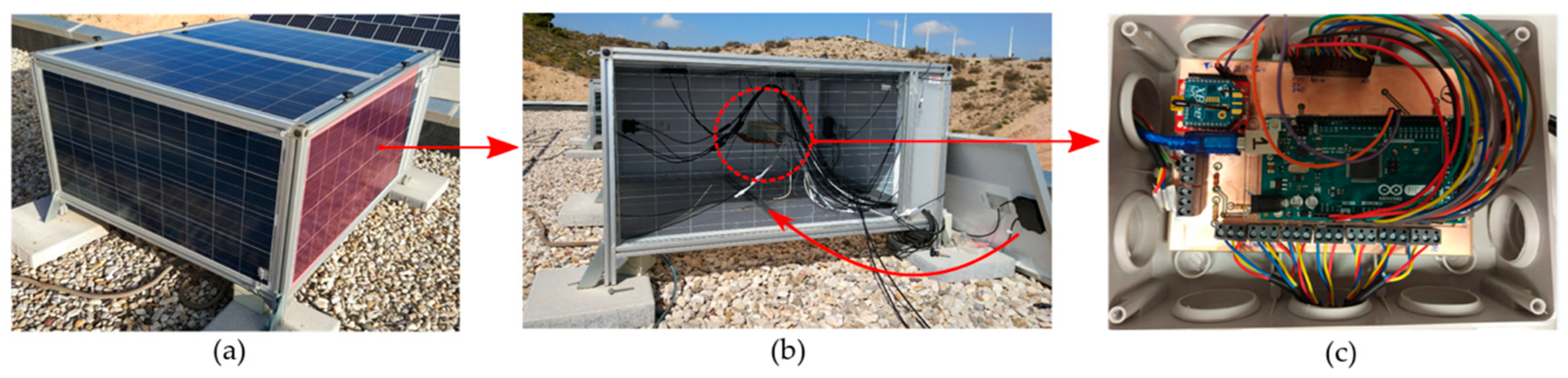
A simple model for a building integrated photovoltaic (BIPV) system was constructed using crystalline silicon modules (Model Atersa SHS100-36P, 100 W_p) in an orthohedric structure, made by the modules themselves and the included minimum additional materials (aluminium frame and polycarbonate small patches, see Figure 1a) [26]. The purpose for the model is to study the temperature behavior of the so-called “PVCube”, working as a long-term module in an outdoor facility, in which the environmental parameters are continuously monitored, thus reproducing the real working conditions of PV modules used as BIPV elements.

Thermal monitorization of the c-Si PVCube’s different faces provides information about the module temperature. In this case of study, the module orientations were: Vertical inclination (90°) with different azimuth (east, west and south) and horizontal (0°), but the methodology can be applied to any orientation (which is especially useful for BIPV systems).

The BIPV test facility was located at 38°01′24″ N and 1°10′32″ W, on the roof of one of the 12 m high buildings at the University of Murcia (Spain), and it collects the temperature of each face (inner and outer), together with the temperature inside the cube, in order to monitor the thermal evolution during the day and night. These data are complemented with environment data (global and diffuse irradiance for horizontal plane, wind speed and direction at a 2 m elevation from the roof, ambient temperature and humidity) measured with a weather station and a pyranometer located very close to the facility. The facility has been in operation since July 2017, with a sampling rate of five minutes. It has been running continuously since then, thus providing an extensive database for detailed analysis. Determination of the electrical parameters (I-V characterization) was carried out using an I-V tracer. Details about the monitoring system, data collection and analysis are provided below.

2.1.1. Monitoring System

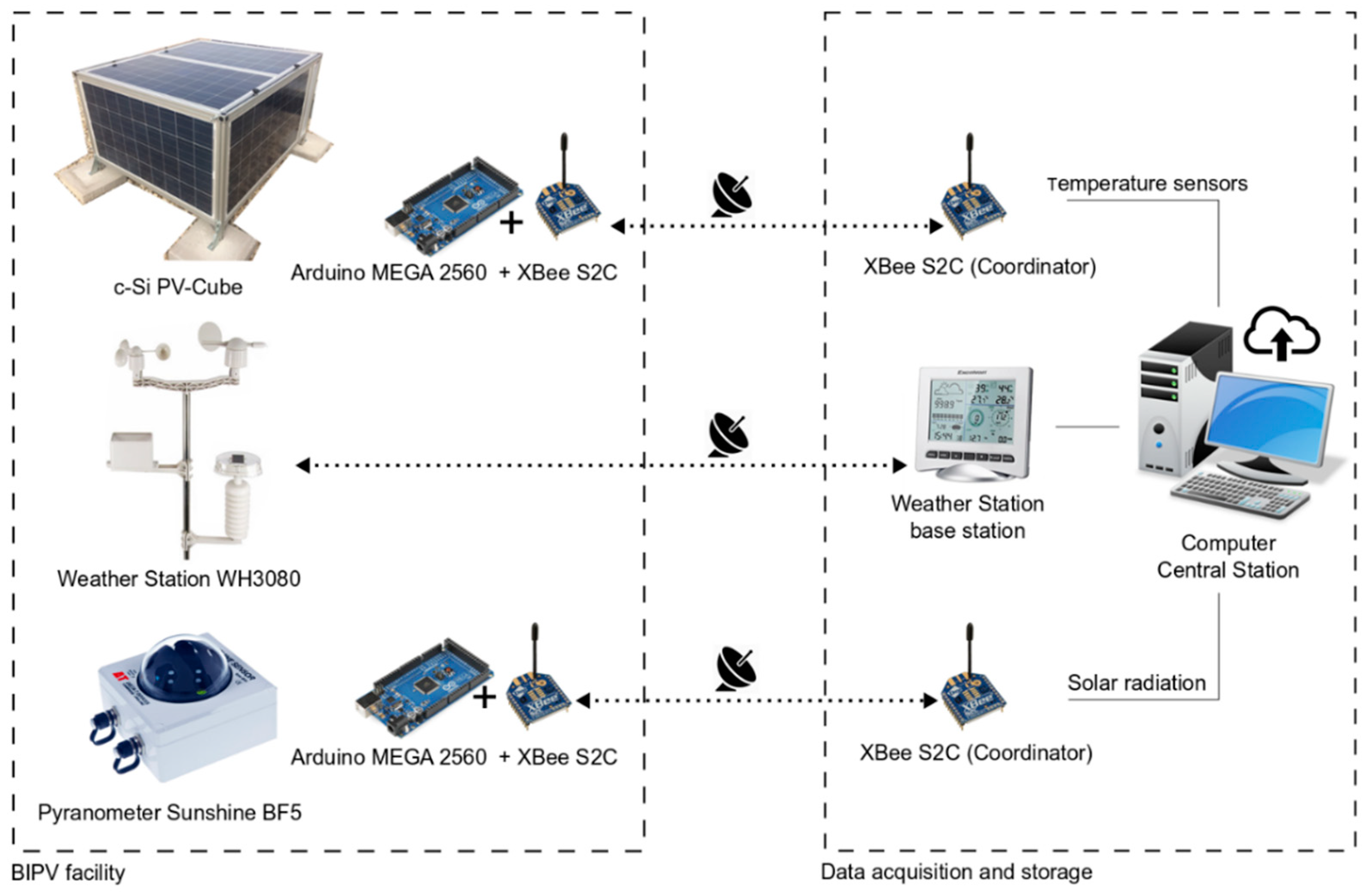
A wireless sensor network, using the ZigBee protocol, has been built to monitor in real time the thermal response of the PV modules. The system is low cost, features easy placement and installation, and is scalable in terms of the number of sensors nodes. DS18B20 and DTH11 temperature and humidity sensors were used to obtain the temperature of each PV module and the temperature and humidity from the inside of the PVCube, respectively. The monitoring system works by combining an Arduino board (model MEGA 2560) and Xbee radio frequency communication module (model S2C), both connected to a home-made printed circuit board for power supply and easy connection of all the sensors. Everything is installed in a sealed box inside of the PVCube (see Figure 1b,c). The network is completed by adding another sensor node with the data collected by the pyranometer (model Sunshine BF5) and adding the Xbee modules (configured as coordinators), which are connected to a PC located at the laboratory on the lower floor below the rooftop, where all the data is saved to a text file using the serial terminal program Coolterm [27].

The environment data was supplied from the weather station (model Froggit WH3080) installed close to the test bench. It transmits the ambient temperature, humidity, wind and rain data to its base station, located in the same laboratory as the temperature and irradiance data logger. It banks up to 4080 sets of weather data in non-volatile memory which is stored in the same database before the oldest data sets will be overwritten by the new ones entered.

Irradiance has been measured using a single sensor in the horizontal position and then the irradiance for different orientations has been calculated. The irradiance measurement and calculations were compared with the data provided by the photovoltaic geographical information system (PVGIS) [28] for the same location. Since the solar radiation data is measured on a horizontal plane, the estimation of the incident irradiance for the other surfaces of interest is based on applying Muneer’s method [29]. The model distinguishes between clear and overcast sky conditions and sunlit and shaded surfaces, and it is one of the most used anisotropic irradiance models implemented in recognized databases such as the PVGIS. The global irradiance provided by the pyranometer and its diffuse and beam components, respectively, was used as the input data. The reflected irradiance was assumed as isotropic, considering the value of 0.2 for the ground’s albedo (gravel roof). The accuracy and range of each of the measured parameters is detailed in

Table 1. Technical specification of the monitoring system for the BIPV facility.

Variable	Range	Accuracy
Ambient temperature	−40–50 °C	±1 °C
Outdoor relative humidity	1–99%	±5%
Rainfall	0–9999 mm	±1.5 mm
Wind speed	0–50 m·s−1	±1 m·s−1 (wind speed <5 m·s−1) ±10% (wind speed >5 m·s−1)
Solar radiation	0–1250 W·m−2	±5 W·m−2
PV temperature	−55–125 °C	±0.5 °C
Indoor PV-Cube relative humidity	20–80%	±5%

. The system’s basic architecture is shown in Figure 2.

In addition, the electrical parameters of the PV modules were collected manually from an I-V tracer (model PVPM 1000CX) which generates an IV curve of 100 points using the 4-wire method. The device has an integrated battery charger and its own industrial miniature PC that transfers the measurements to the database of the PVCube for further analysis. The data acquired are then processed and compared with references curves provided by the manufacturer.

2.1.2. Data Analysis and Failure Detection

The recorded data was then processed to create models and generate statistics. The dataset that was created was based on the monthly files stored in the computer central station, which has an internet connection that provides remote access to the information. For management of the three databases (PV temperature sensors, solar radiation and meteorological data), a MATLAB code was developed. The program extracts and filters the data to export a single file as demanded. Ideally, the data should have been measured exactly at the same time. However, individual parts of the monitoring system were not synchronized due to the pre-established sampling rate. In order to have the same timestamps, the closest two measurements in time from the weather station and pyranometer were selected. The time difference had to be less than 15 min, and if there was no applicable data, the data regarding the environmental conditions (both solar radiation and weather station) was dismissed. If both values were correct, the PV temperature sensors from the PVcube were added to the meteorological variables, applying a linear interpolation. After this step, a new matrix was generated, all with the same timestamp and number of data to export to a single file.

Predictive model approaches for the BIPV system were based on the comparison between the measured and modelled I-V curve of each PV panel using the one-diode equivalent electrical model and fitting the standard parameters of the equivalent circuit.

The fault diagnosis procedure was carried out in two steps, firstly, the characterization of the PV module using the I-V tracer was carried out. Secondly, a modelled I-V curve is then compared with the measured one, detecting deviations between the predicted model and the observation, and finally, considering the deformation of the I-V curves, the failure is identified. The mismatch between the simulated (set-up as a reference) and measured I-V curves allows the identification of different classifications of failures [15,16,17].

The simulation extracts one-diode model parameters under a MATLAB environment using a PVSYST software model [30,31].

2.2. CdTe Parking

A 222.36 kW_p photovoltaic system was built as part of a parking garage roof at the University of Murcia campus, located at 38°01′12″ N and 1°09′56″ W [32]. The system was built during late 2008 and the beginning of 2009 and was finally commissioned in May 2009. The yearly average daily irradiation is 5320 Wh·m⁻² [28], which is similar to the average measured by our monitoring system, which is 4960.17 Wh·m⁻² per day. The system is comprised of 3144 CdTe First Solar modules, with an orientation of 20° east and a tilt of 7° over horizontal in order to avoid shadows between the three sectors in which the structure is divided. The 30 single-phase inverters are SMA (model SMC 7000HV), with 7 kW of capacity, and are grouped in order to generate a three-phase alternating current signal. A SensorBox^® (SMA Solar Technology AG, Niestetal, Germany) data collector system is used to collect data which are transmitted through an RS-485 data network. The inverter manufacturer offers a proprietary data logger component to access to this RS-485 network.

In this study, we developed a data acquisition system to gather and analyse information from the 222 kWp thin film CdTe parking integrated grid-connected photovoltaic generator, which sends several data to a server at a sampling rate of five minutes. The data includes technical information such as net frequency, direct current, delivered AC power, PV input voltage (at maximum power point), date and time, etc., as well as meteorological information, i.e., global irradiation, environmental temperature and solar module temperature. Further details regarding the generator and its configuration can be found in the work by Serrano et al. [32].

Data computing learning techniques were applied to the large stored datasets. Computational techniques let us classify the performance of the generator, dealing with the failures or errors that may occur, namely shadows, dirty modules, inverter failure, etc., with the aim of building a predictive diagnosis system. The comparison between different groups of modules performance, as well as the whole system performance, provides information to identify possible errors. Data mining (DM) techniques develop models to discover unknown patterns in data, as part of knowledge discovery in dataset (KDD) processes. We applied DM techniques to the stored data from the photovoltaic generator to get a classifier, which was tested to assess its accuracy. The process required experts to examine each dataset to set the state of the generator determined by a label, and so identifying the possible causes of a group having lower performance than its neighbors.

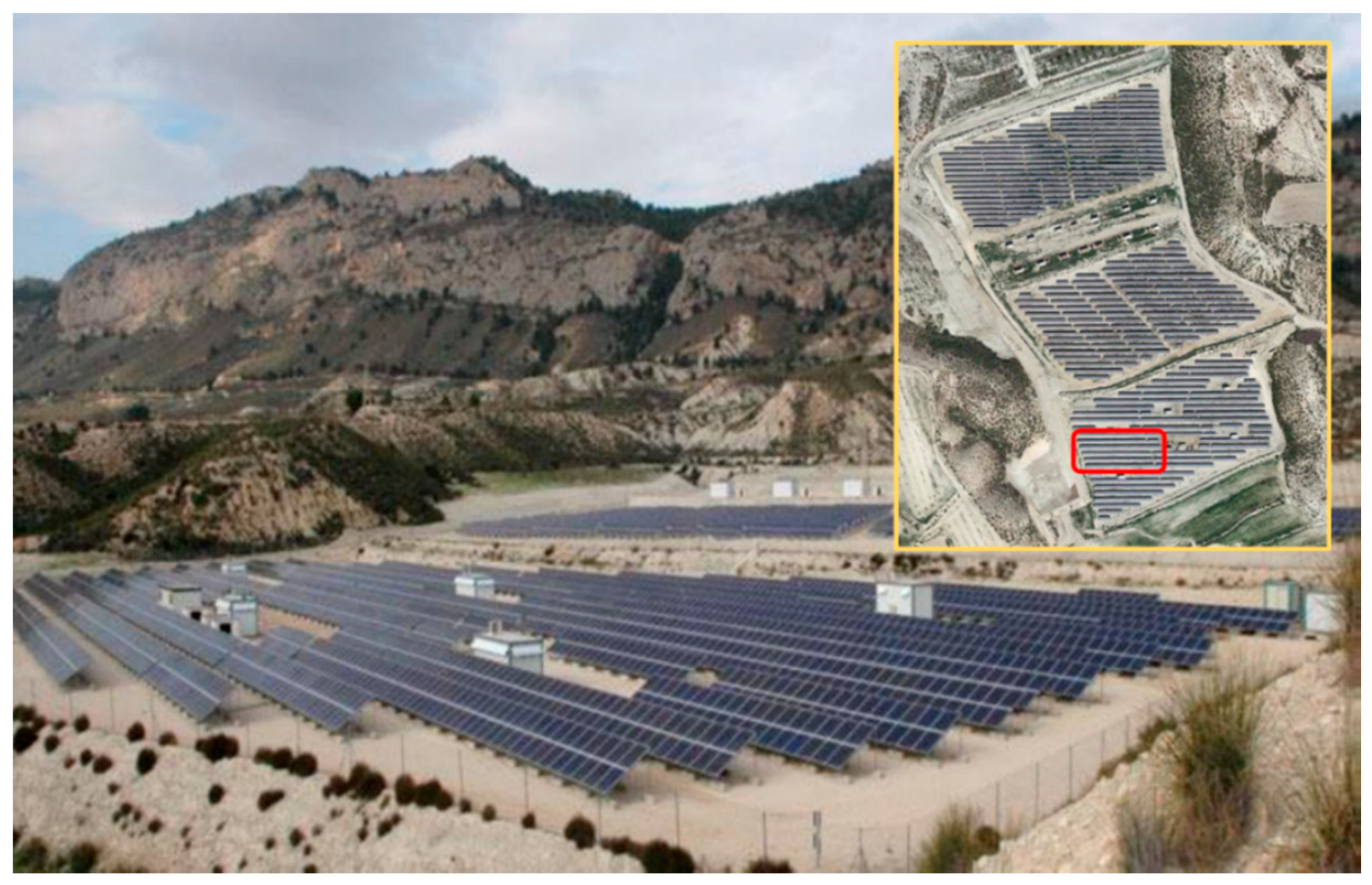
2.3. Yéchar Solar Plant

The Yéchar Solar Plant in Murcia (Spain) is located at 38°5′36″ N and 1°26′37″ W and has a nominal installed capacity of 2.12 MW_p. The plant is organized in three main phases of 710 kW_p, each comprised of several strings which are connected to 276 inverters of different sizes. The three phases were inaugurated in 2005 (May), 2006 (October) and 2008 (July). All the inverters were manufactured by Fronius, with different nominal outputs of AC power, as detailed in

Table 2. Description of the 276 inverters installed in the Yéchar solar photovoltaic plant. The model, nominal maximum output AC power, number installed and total power per each model of inverter and total per the plant are provided.

FRONIUS Inverter Model	Nominal Output Power (max. kW AC)	Number Installed	Total Power (kW AC)
20	2	10	20
30	2.65	69	182.85
40	4.1	3	12.3
60	5	171	855
300	34	1	34
400	42	20	840
PLUS 55V-1	5	1	5
PRIMO 5.0-1	5	1	5
Total:	---	276	1954.15

. The distribution of inverters in the three phases of the plant is very similar, with only one difference between them regarding the largest inverters of 42 kW (Fronius Model 400): Three were installed in the first phase, six in the second one and eleven in the third one (plus the 34 kW Fronius Model 300 inverter).

In the solar plant, a policy of monitoring the inverters was applied from the beginning, and the summary of failures up to the end of 2015 is presented in this article. All the inverters are monitored, and within ten years of operation, 66 of them have presented failures. Those installed in the third phase presented failures within eight years (a difference significantly applicable to the 42 kW inverters). The inverters presented several failures in the different components, and the statistics depending on the failure per inverter model and failures over total inverters were collected.

The plant is comprised of 12,885 Photowatt Si multicrystalline photovoltaic modules (Series PW1650, with solar cells of good power conversion efficiency, 15%). The modules have a STC nominal power output mainly of 175 W_p (2376 modules) and 165 W_p (9215), with a minor number of 160 W_p (205), 155 W_p (108), 145 W_p (122), 140 W_p (811) and 125 W_p (48) nominal power outputs, providing a total output power for the solar plant of 2.12 MW_p, organized in three phases of 710 kW_p.

The inspection by thermal camera was carried out manually on a sector of the plant comprising 245 modules (PW1650, 165 W_p). The inspected sector, indicated by a red rectangle in the inset of Figure 3, is shown alongside a picture of the plant. The inspection was carried out in 2017, eleven years after the installation of the modules. A thermocamera was used to take individual pictures of each module. The camera was a FLIR TAU2 model with a resolution of 640 × 512 pixels (pixel pitch 17 µm), a sensitivity of <30 mK, a spectral band of 7.5–13.5 μm, a scene range (high gain) of −25–100 °C and a scene range (low gain) of −40–550 °C, providing enough resolution and accuracy to detect temperature gradients within individual solar cells. The “Flir Tools” software was used for the image analysis. All of the thermographic pictures were taken with irradiance levels higher than 800 W·m⁻², and the camera was calibrated and the emissivity factor was determined by random sampling of several modules, providing a value ε = 0.75, which was used to assign temperature values to all of the thermographic images.

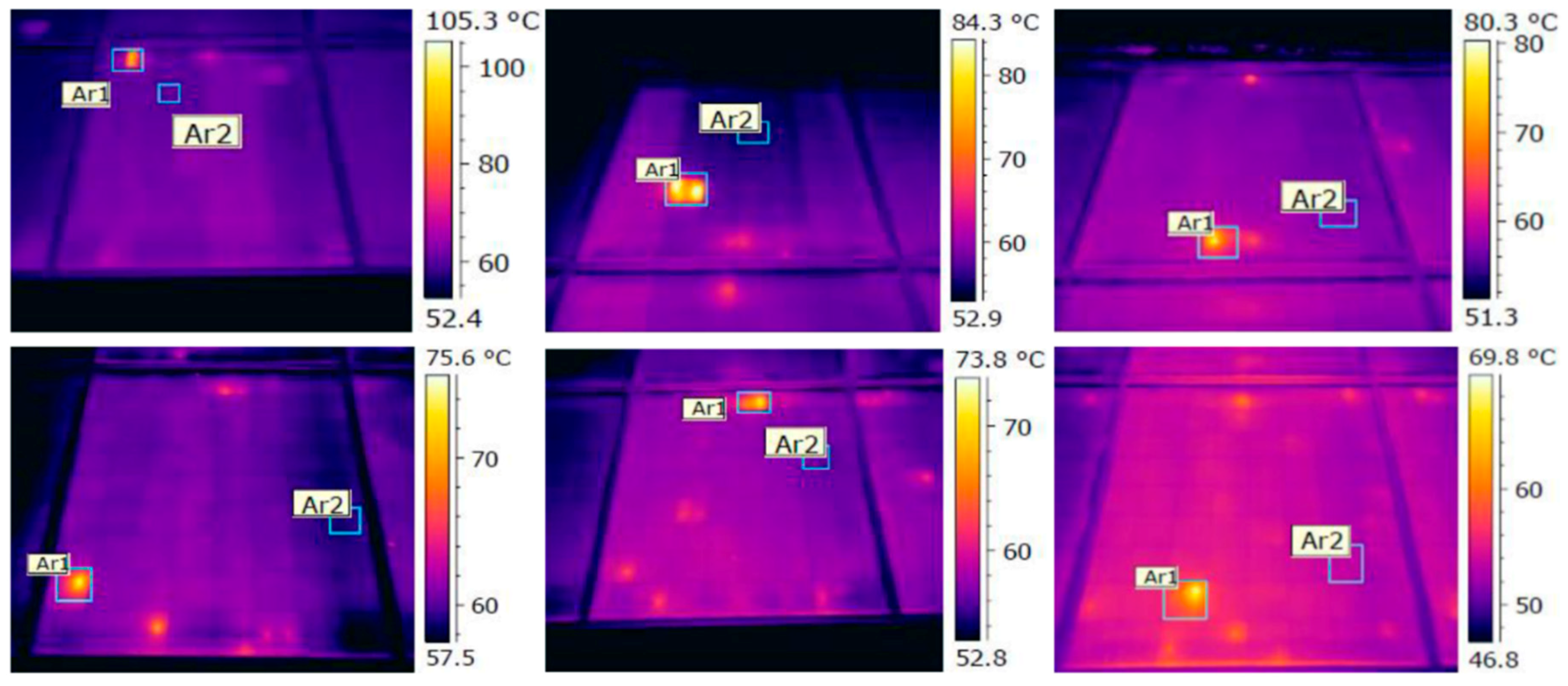
In the thermographs, two areas are stablished, one containing the highest temperature region and the other one as a representative of the mean temperature of the module, considered as the “background” (both areas are indicated by the Ar1 and Ar2 labels, respectively, in the thermographs of figure presented in Section 3.2). The two maximal temperatures within each area were compared and a temperature difference (ΔT) between them was stablished. The classification of the faults was accomplished according to the size of this gradient: ΔT > 30 °C (grave fault), 30 °C > ΔT > 15 °C (medium fault) and 15 °C > ΔT > 5 °C (light fault), while for ΔT < 5 °C it is considered normal behavior. The classification was based on the research of Buerhop et al. [22]. The failure patterns of PV modules was determined with the IR image given by the International Energy Agency (IEA) [16], and the algorithm for fault diagnosis by Menendez et al. [24], which discards all temperature differences that are not more than 5 °C, was based on empirical analysis.

3. Results

Different kinds of results have been obtained for the three PV systems presented above and the analysis of the data has been carried out using different methodologies. Nevertheless, when presented as a whole, methodologies provide a progression which clearly indicates which one is the optimum monitorization strategy, depending on the scale of the system, always with the purpose of detecting failures and proceeding with the best maintenance strategy for each case. In this section, we present the results for the three case studies, but they are organized depending on the failure detection method which was applied, namely predictive modelling based on the technical and environmental parameters (for the c-Si PVCube and CdTe PV parking garage) or failure detection based on cross-correlated data analysis, which does not require modelling (CdTe PV parking garage and Yéchar solar plant).

3.1. Results Based on Predictive Modelling

The common characteristic of this kind of results is that they are obtained by comparing experimental data with modelling carried out using the environmental parameters measured in real time. Technical parameters are obtained by fitting the equivalent one-diode circuit model (starting with the parameter values supplied by the manufacturing company) and using environmental parameters (measured using the monitorization system). The deviations between the model calculation and the measured full I-V curves (or voltage and power output at maximum power point) provide information about possible failure. Detection and classification is carried out by the data analysis of those deviations.

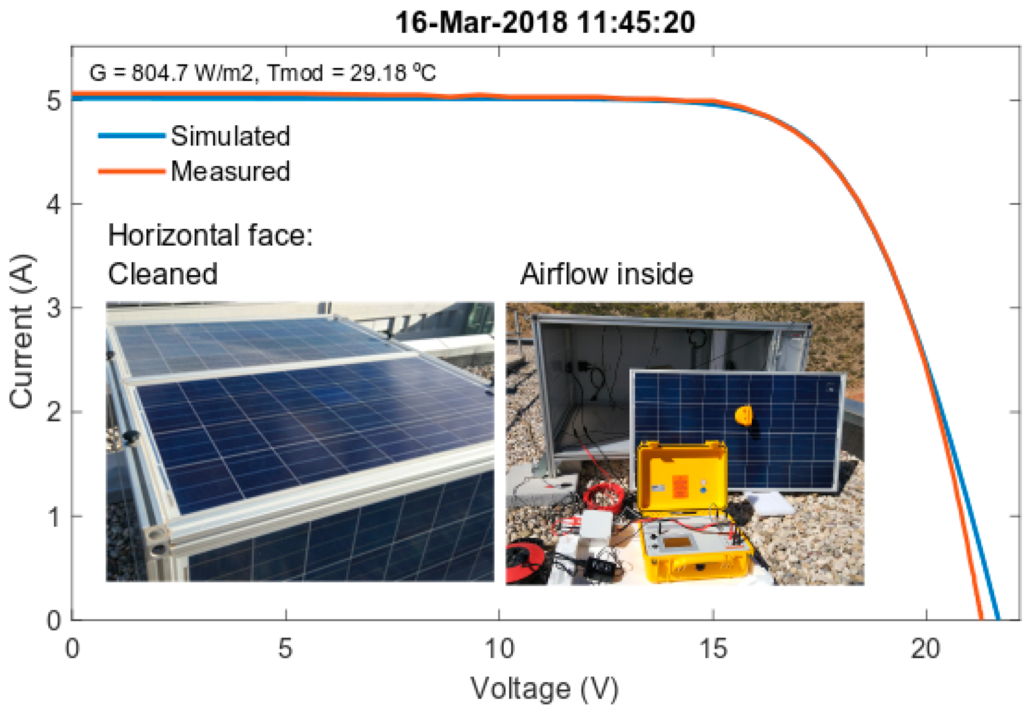
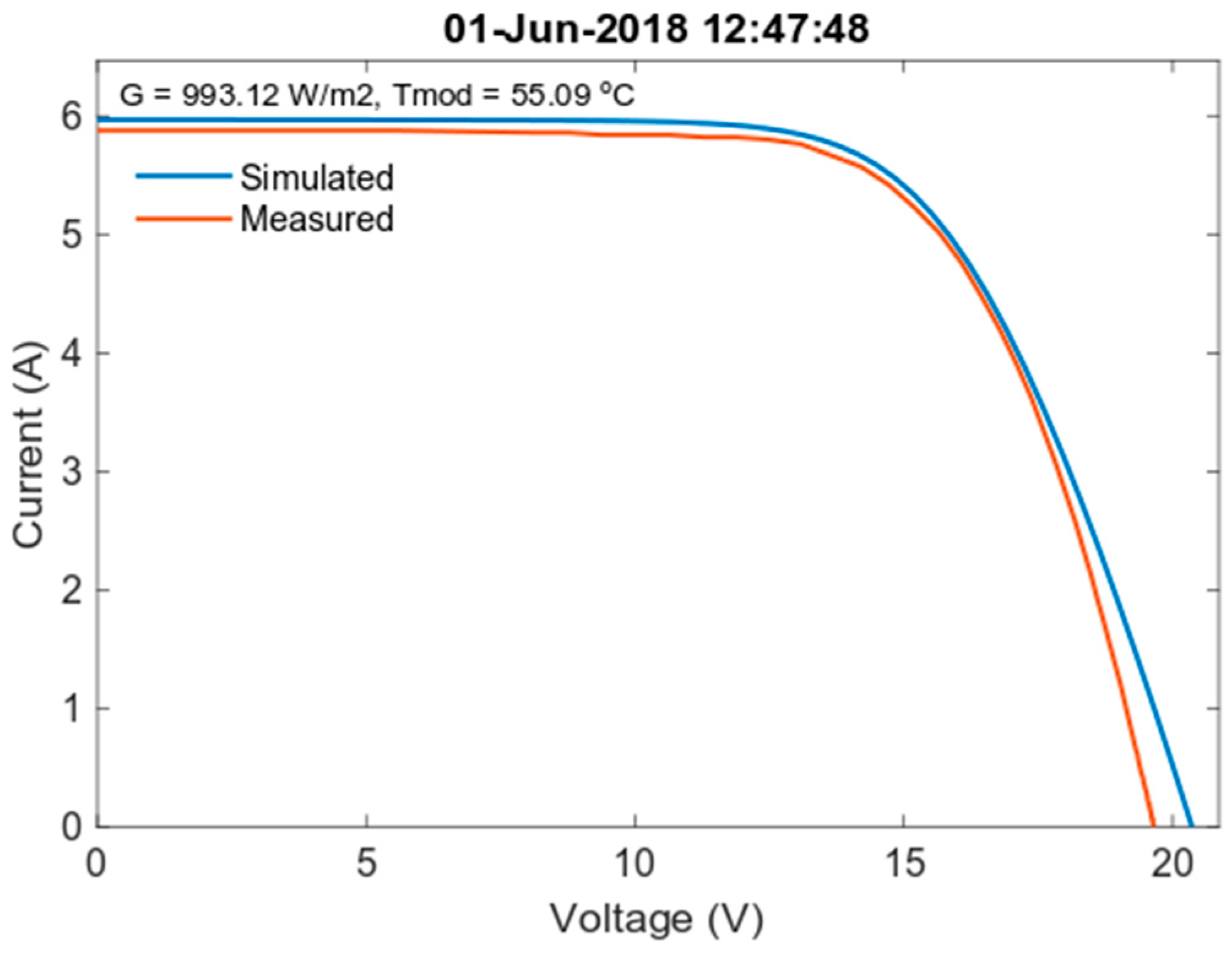
Regarding the c-Si PVCube, Figure 4 shows an example for the measured and simulated I-V curves for the horizontal face of the cube when the PV module was cleaned and one face was opened, allowing airflow inside of the structure. There was a slight lost in the experimental Voc (+1.8%), likely caused by measurement error. The behavior of the cube when there is not airflow inside (all the faces closed, fully integrated) presents a dramatic increase in module temperature, and consequently the thermal stress of the structure, which is correlated with the in-plane irradiance. 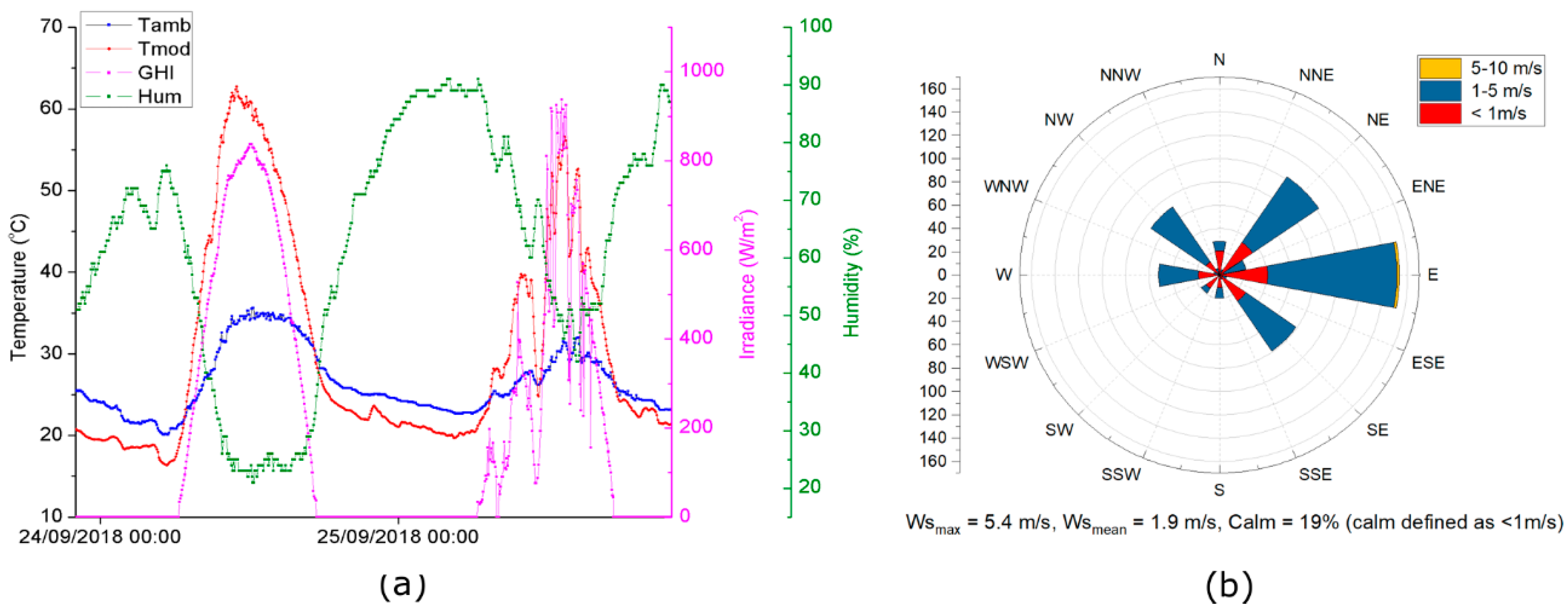Figure 5 shows an example of the thermal and ambient parameters, monitored for 48 h, which were used to analyze the thermal evolution on the inner horizontal module and its dependence on ambient conditions, such as irradiance, ambient temperature, relative humidity and wind speed. Two typical days are shown: Clear and cloudy. In this case, the difference between the ambient and module temperature during night time is close to 5 °C, but during daytime, the module temperature differs up to 20 °C compared to ambient temperature, when the received irradiance has a value close to 800 W·m⁻².

Figure 6 shows the measured and simulated I-V curves for the horizontal surface when the PV module is fully integrated (there is no airflow inside the PVCube) after two days of rainfall. The DC power output that was measured had a deviation of −1.7% from the reference value. Despite the difference between the model and predicted output not being considerable, since the system has been working for about 15 months, slight differences from the reference model can provide information about potential faults in the system and degradation processes. For instance, the slightly lower short-circuit current is likely caused by the dust, which blocks irradiation. This information can be relevant in the establishment of the corrective maintenance, defining a threshold where actions are required. On the other hand, the evident reduction of the open circuit voltage as a result of a short circuit fault is likely caused by thermal stress (high working temperatures and poor air ventilation), which affects the junction box and therefore the bypass diodes. This behavior for BIPV systems has previously been reported by Spertino et al. [33].

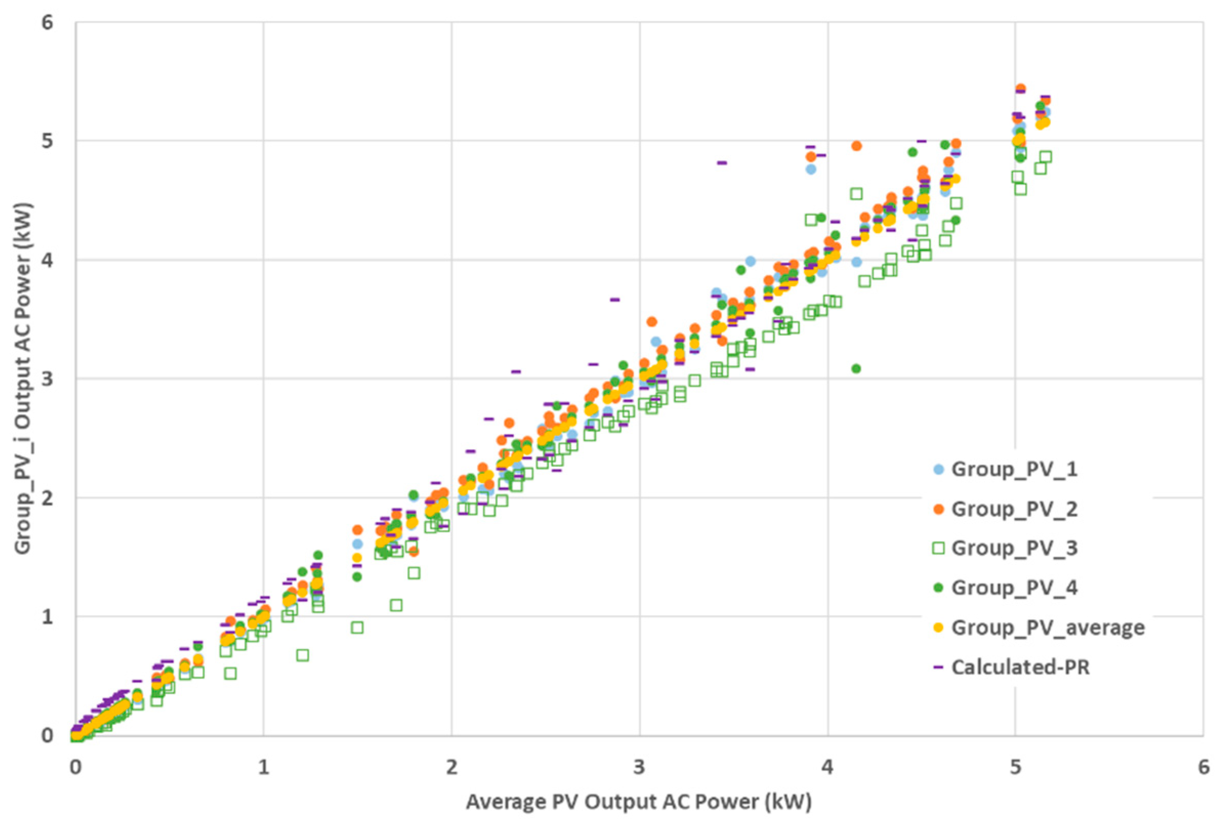
Similar modelling procedure can be applied to the CdTe PV parking garage system. In this case, using environmental parameters, a model is applied to obtain the maximum power point for a given irradiance and temperature (which are measured) using the manufacturer technical parameters. Detection of faulty “strings” can be obtained, since the power output is aggregated by the inverter for each string of modules. A set of calculated and measured maximum power points is presented in Figure 7 (purple bars). For strings that are working correctly, the difference is small, while for faulty strings, the comparison of both values easily provides an “alert”, indicating that this particular string is failing (open green squares in Figure 7). The detection of the exact module (or modules) which is (are) failing in this case will require special measurement of individual modules, which is a manual maintenance procedure once the faulty string has been automatically detected.

It can also be appreciated that the modelling based on a performance ratio which depends on irradiance and temperature is correct, but in this case, it has considered a single constant value for the efficiency of the AC inverter (“European” efficiency) while the real curves for the inverter efficiency show a drop in its value for lower outputs of converted AC power. This is the reason why the modelling is more accurate for higher irradiances (and therefore power conversion closer to the nominal maximum power of the inverter) and shows an overcalculation for irradiances lower than 250 W·m⁻².

3.2. Results Based on Cross-Correlated Methods

In this case, three sets of results are presented, the first one regarding the CdTe PV parking system, based on the analysis of data provided by the inverters and two others regarding the Yéchar solar plant: Inverter failures and thermographic module failure detection.

For the CdTe PV parking garage system, the monitorization of the SMA inverters provides a large database of several parameters that can be cross-correlated using simple computing algorithms. The main difficulty is organizing the database, which due to the large size may require data mining techniques. Using this information provided by the inverters, both failure detection and failure classification can be carried out without the need to compare with theoretical models, which require the input of environmental parameters or module parameters.

The reasons why different groups of modules behave differently under the same environmental conditions could be key to find algorithms that are able to identify and predict failures, or to point out dirty modules or hot spots.

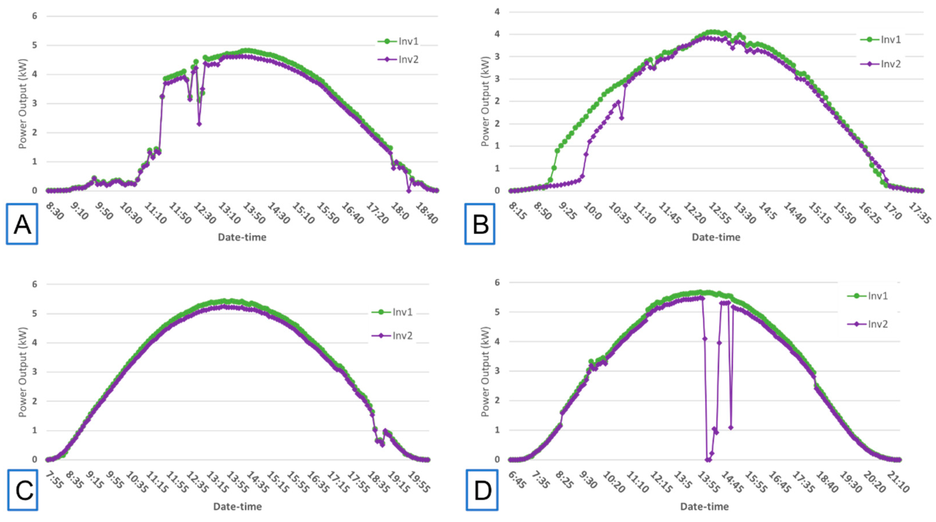
From the stored datasets, there are chances to identify real time performance faults or inefficiencies without the use of environmental data or solar cell modelling. Figure 8 shows the power output of two different PV modules groups which are technically identical and are simultaneously measured under the same environmental conditions (irradiance, temperature and wind). It is already obvious that one of the strings is underperforming, but also instantaneous faults can be easily detected, as can be seen in the loss of power output in Figure 8D for one of the inverters. Single faulty events can be undetected unless an automated alarm is triggered in the inverter, and only a data treatment of a larger time span enables reliable failure detection. 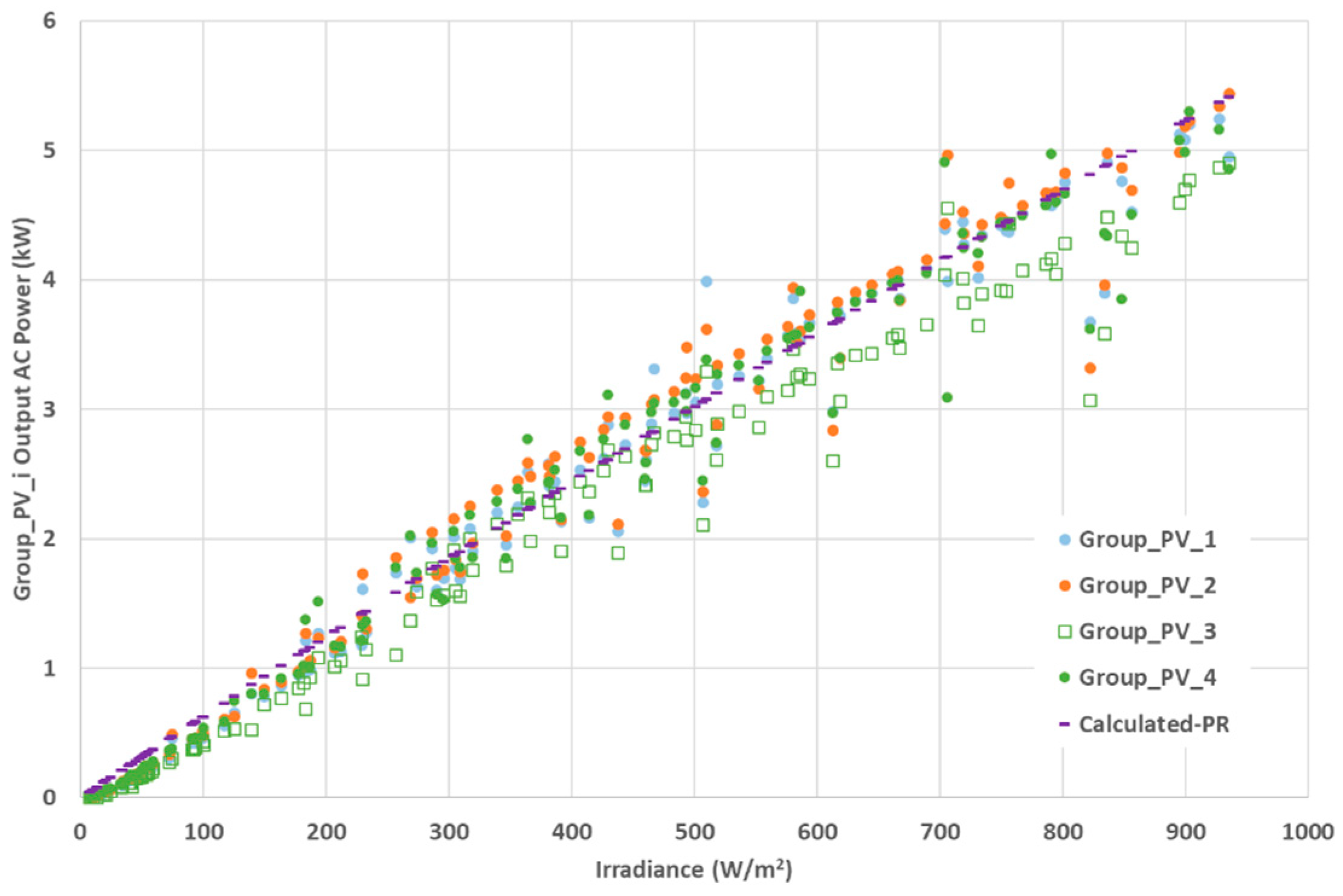Furthermore, in Figure 9, the cross-correlation of the string’s power output provides a fast and clear method to detect failing strings. This procedure does not require any kind of modelling and simple algorithms can be applied to cross-correlate all strings with other strings or the mean value of all strings (ideally excluding the one being compared). The lower power generation shown in Figure 8 and Figure 9 for the behavior of Inv2 could indicate the shade effect, the soiling effect, or the mismatching effect in the solar array, for example.

This method of cross-correlation for a massive amount of data is very reliable, as can be seen in Figure 9, where the faulty string (Group 4, green open squares) is showing a strong underperformance when compared with the other groups or the average value of several groups at all output powers. This kind of failure is not detected automatically by the single inverter, since the group is behaving correctly. The theoretical output presented in the previous section is also superimposed in Figure 9, to show how the identification of the faulty string is clearer with the cross-correlation than the modelling (as shown by comparing Figure 8 and Figure 9) due to the uncertainty in the technical parameters and the measurement of the environmental magnitudes used for the model calculation.

This mechanism detects and identifies the failures, and so the reaction to repair or find a solution is fast. Further computational techniques can be applied to find an algorithm that is able to predict the errors/failures before they appear, using machine learning techniques and thus providing chances to avoid them before they can be converted into fatal failures.

The second set of results, which illustrates the cross-correlated methods, uses thermographs of a sector of the Yéchar solar plant. The results of the thermographic pictures, taken manually on 245 modules of the Yéchar solar plant, have been classified and analyzed. Following the classification criteria explained in the methodological section, several modules which presented grave, medium and light failures were detected. The results are summarized in

Table 3. Statistics of failures in photovoltaic modules detected by thermography in a 245 module sector of the Yéchar solar plant. Percentages are shown for the kind of failure and proportion of overall total number of inspected modules. Last column: An extrapolation of possible failed modules, taking into account the total number of modules (12,885) and the statistics of previous columns.

Kind of Failure	Number of Failed Modules	% Kind of Failure	% Failed Modules	Extrapolated Number of Failed Modules (Whole Plant)
Grave failures (ΔT > 30 °C)	1	1.5%	0.4%	53
Medium failures (15 °C < ΔT < 30 °C)	6	9.1%	2.4%	316
Light failures (5 °C < ΔT < 15 °C)	59	89.4%	24.1%	3103
Totals:	66	100%	26.9%	3471

, where the statistics of failed modules are presented and the extrapolation to the whole plant is included in the last column. The sample of inspected modules was randomly selected and therefore a linear extrapolation was carried out to calculate the total number of modules that may be failing in the whole plant (presented in the last column of Table 3).

In Figure 10, thermographs of six panels in which failures were detected by temperature gradients are shown. Two areas are indicated in each picture: One containing the highest temperature (Ar1) and other containing a medium-low temperature area (Ar2). The maximum temperature within each area was compared and a gradient was obtained and used to classify the failures. Only six representative images showing clearly the presence of overheating are shown here. A total of 245 thermographs were obtained, with 66 of them showing a ΔT larger than 5 °C.

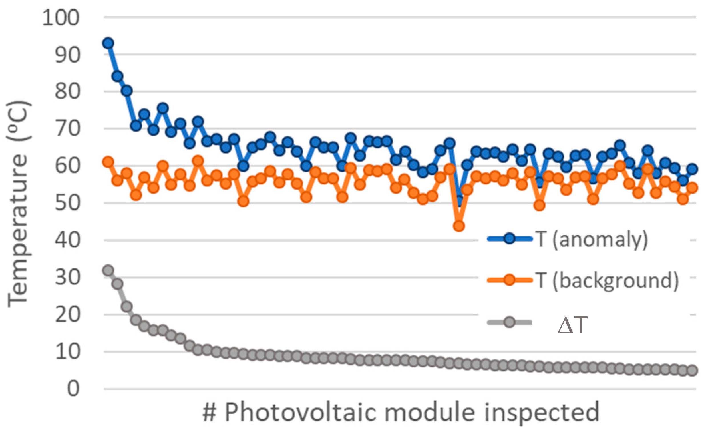
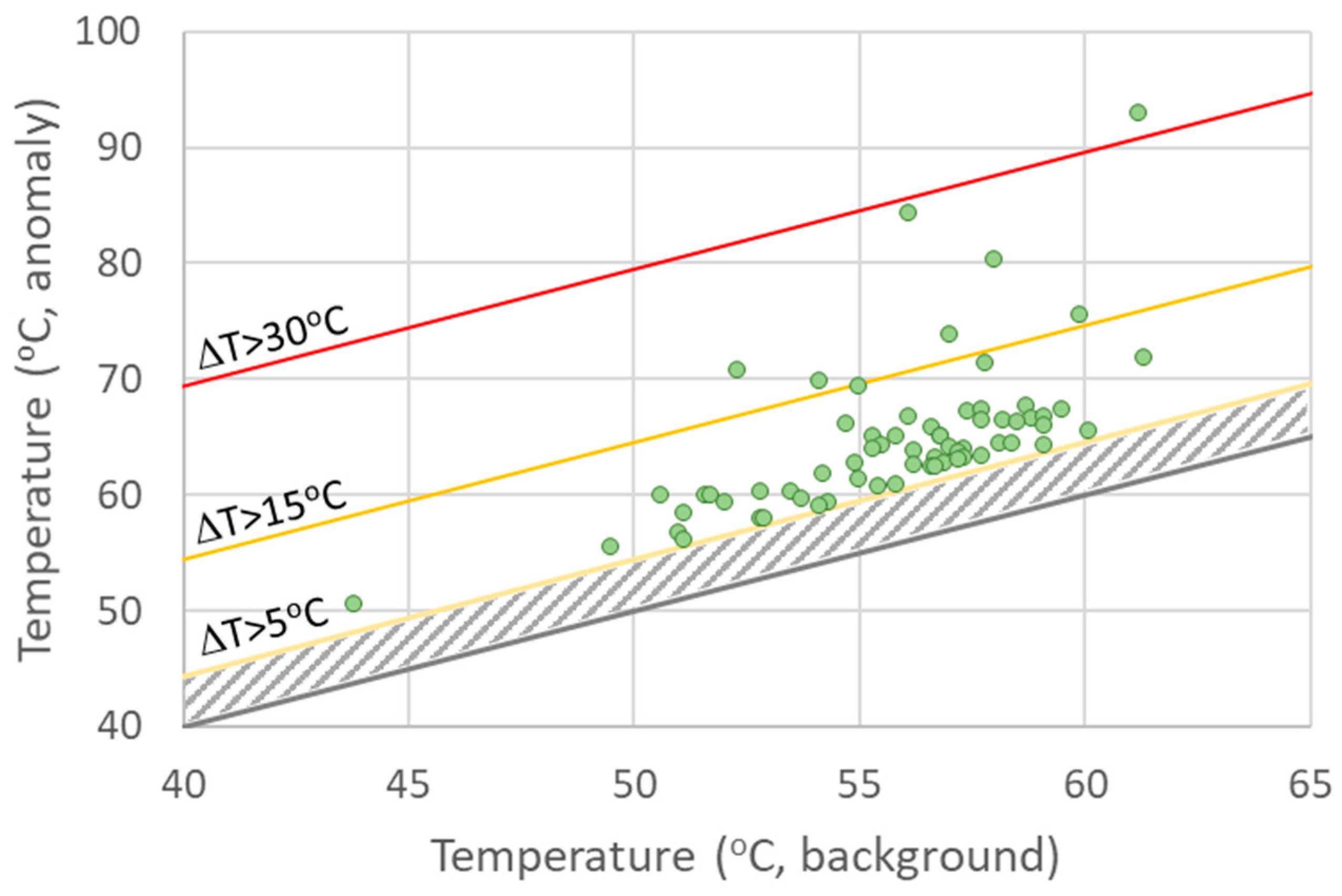
Figure 11 and Figure 12 show the distribution of temperatures between the anomaly and background areas of all 66 modules which can be considered as failures according to the criteria explained in the methodology section. In Figure 11, the distribution of temperatures is shown (ordered by the amount of ΔT, from higher to lower, left to right), with only a few modules showing temperatures above 70 °C. All of them have a very large ΔT (grave or medium fault). In Figure 12, a cross-correlated plot is presented, and the distribution of failures can be easily identified by the superimposed lines marking ΔT in excess of 5 °C, 15 °C and 30 °C, respectively. A certain correlation is shown which relates the higher range in module temperature with higher ΔT, but it cannot be considered a consolidated trend due to the dispersion of the data. All modules inspected with ΔT < 5 °C will be in the grey striped area. Once the modules with grave and medium failures were detected, visual inspection of the modules indicated that the grave failure were due to a fractured cell, the medium failures also included a fractured cell, but all others failed due to failure of the welding of string contacts within the module. In the remaining 59 light failures, all but four were string welding problems, the four remaining being a problem with the connection box between modules (three cases) and a possible problem with the bypass diode (one case).

As a conclusion, and apart from the broken cells (only two), it can be said that all failures were due to problems in the soldering of string contacts within the modules. A replacement of the seven modules with grave and medium failures (53 and 316, respectively, if we extrapolate to the whole plant) will be a quick and easy maintenance procedure that will improve the performance ratio of the solar plant. In this case, a more automated procedure to locate the failing modules in the whole plant should be developed, since a manual procedure cannot be applied easily at very large scale, as commented in the discussion section.

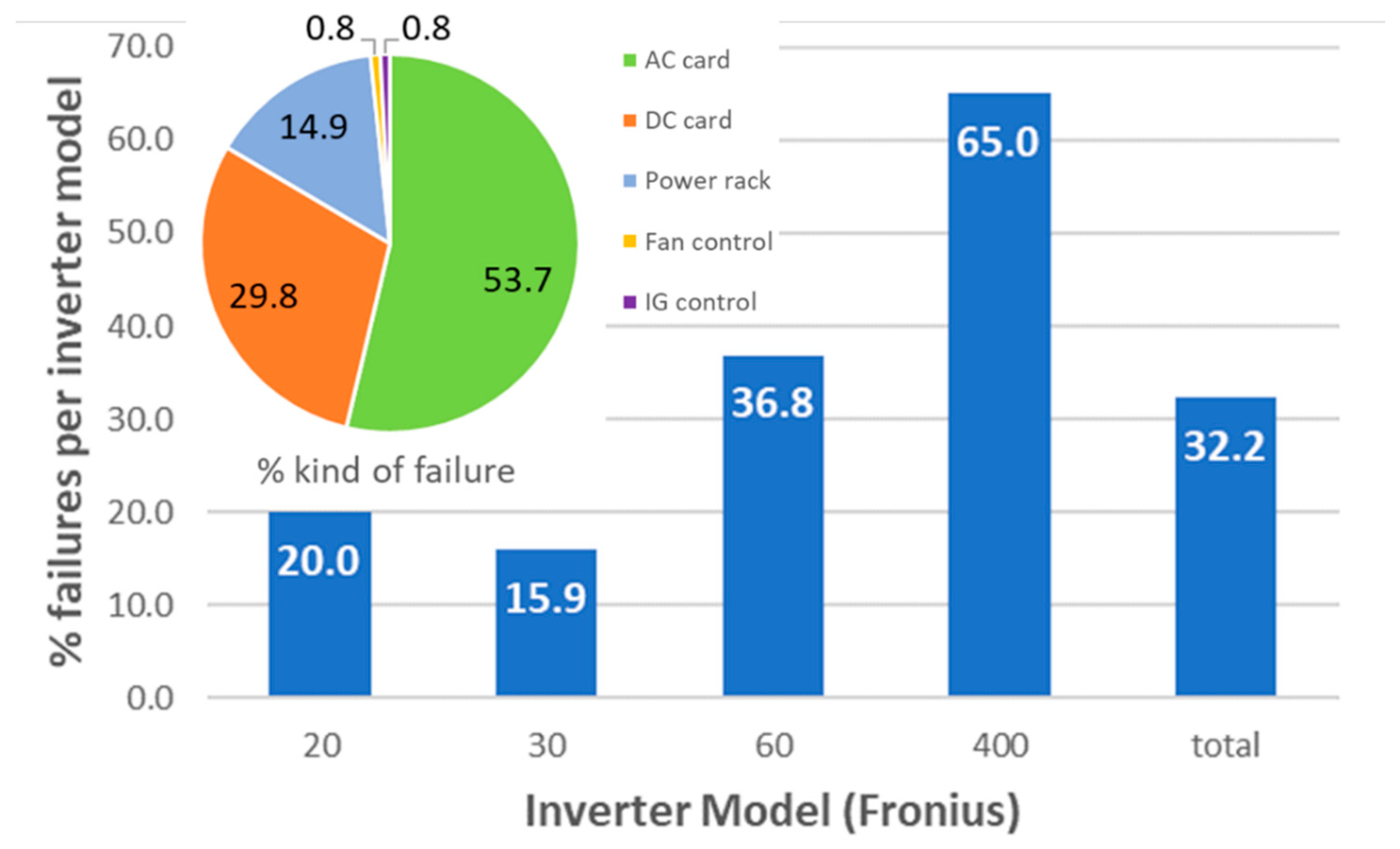
Finally, and also focused on the Yéchar solar plant, the failures detected in the Fronius inverters are summarized in Figure 13. The number of failures was high after ten years of operation, providing an average of 32.2% between all models, with a special incidence of high power inverters (65%, with failures in the power stage). The number of inverters inspected was high (279), providing significance to the statistical values, especially for models 30 and 60, which were the most used. All of the inverters have been working in the same environmental conditions, and therefore this sample is very useful to test the reliability of models from the same manufacturer. From this study, it is clear that smaller inverters are more reliable. The distribution of failures is included as a pie chart inset in Figure 13. The AC card (53%) and DC card (29.8%) failures (percentages over total number of failures detected) are the parts which required more reparations, followed by the power racks (14.9%, over total, but with special incidence in the largest model 400 inverters, as can also be seen from the 65% of them which failed). Reparation of the inverters requires manual operation and it is therefore expensive. Preventive detection for this kind of failure will require analysis of trends of power output and machine learning procedures to provide alert signals before the actual failure occurs.

4. Discussion

The results of the case studies presented in this article, although at very different scales, allow us to recommend a general methodology that can be applied to monitor any PV system and to detect underperformance and failures in different components, namely photovoltaic modules or strings, and balance of system (BOS) components, especially inverters. For medium or large scale systems, the data provided by the inverters are key to easy, fast and cheap monitorization using cross-correlation of the collected parameters. Only a good communication system and enough data storage (both can be cheap) are required. Then, simple algorithms allow the maintenance team to detect strings with failures or, more easily, failures in the inverters themselves. Regarding module failures, after this initial detection, visual inspection and manual intervention is required to detect the failed module within the string, the same for the problem within the inverter, manual replacement of the damaged component is required. Regarding underperformance with no obvious failure, a more detailed analysis is required, taking into account the degradation of the modules or bad electrical connections. In this case, closer monitoring of the underperforming part of the system is required. If the component that needs to be replaced is a photovoltaic module, this poses a problem if a model with the same parameters that the rest of modules of the string is not available in the market anymore. Even if it is available, it will work with the initial module efficiency, while the other modules remaining in the system will already have experienced some degradation (of the order of 1% losses in power conversion efficiency per year). It is always recommended to proceed to a “revamping” of the system, not only changing the damaged module, but also reorganizing full groups of modules in order to reconnect them in homogeneous strings [34].

If the failure is within the inverter, then the damaged component must be replaced (for example AC or DC cards, which are the main failed component in the monitored Fronius set of inverters in the solar plant, see Figure 13). The cost of this replacement is always high, and most of the time, the component has to be sent to the manufacturer, and in this case, also the cost of opportunity arising from having the inverter offline for several weeks has to be added to the reparation cost (for the mentioned cards, around 800 euros per unit, information from company “CRES” (“Compañía Regional de Energía Solar” (CRES), Avenida Libertad 213, San José de la Vega, 30570 Murcia, Spain). The cost of opportunity is larger for larger inverters. In the case study of the solar plant, the larger inverters also presented a higher statistical number of failures (reaching 65% in ten years), and therefore, the main recommendation arising from this experience is to install medium size inverters (lower than 20 kW maximum AC power). Standardization and developing local markets for inverter spare parts is strongly recommended.

After this initial collection of data by the inverters, the best method to monitor PV systems is taking pictures with a thermal camera. Thermographic images are very reliable to detect failures at a single module level. Automated thermal image analysis provides a fast procedure to classify the kind of failure (grave, medium, light), but also to gain insight about the origin of the failures. In all cases, the anomaly temperature of one single cell (or part of a cell) can be detected by the thermal image. This is not the case for temperature monitorization with thermal sensors, even if used at a single module level (which is possible, but expensive if the solar plant is very large), in Figure 11 it can be seen that the “background” temperature does not indicate any trend, even if the module presents a grave failure: All temperatures are within a band of 50 °C to 60 °C, even if the temperature of the faulty part of the module (“anomaly” temperature) is as high as 93 °C. In order to detect the failures, the thermographic image was needed and the thermal sensor will not have detected the problem.

Furthermore, taking individual module images is not an expensive method (the average cost of per image is 0.12 euros, although person-work time will double this figure, data provided by the company “Drónica” (C/ Berlin, parcela 3-F, Pol. Industrial Cabezo Beaza. 30353 Cartagena, Spain). In this work we have presented data from a sector of the solar plant (245 modules were analyzed), if the whole plant were to be analyzed, the total cost would have been more than 1500 euros for the pictures and around 3000 euros if we consider the person-work required for the analysis of the images. This is not a large amount if we compare it with the benefit of replacing the modules with grave failures, which will boost the performance of the affected string. More automated methods, using cameras installed in drones which fly over the solar plant, taking pictures, plus improved software to process the images will make this method the most competitive [35].

More sophisticated data collection, including environmental parameters and full thermal and electrical parameters of the PV modules can be useful for research purposes or to improve modelling, but the cost and the person-work required is not competitive to monitor large scale systems. Research facilities, or small parts of a larger plant could be monitored in this way in order to increase our knowledge on degradation mechanisms, or to obtain useful information to increase the performance ratio of the systems. Also, analysis of large databases, automatically obtained by collecting and storing parameters measured at inverters or with the thermal sensors or I-V tracers, including environmental parameters, will require data mining techniques and machine learning procedures, in some cases applying artificial intelligence techniques. This computing assisted monitorization will allow researchers to extend in the near future their methods to large scale plants, where data collection and analysis can be fully automated.

As a summary, the best procedure to monitor PV systems in order to detect failures and to proceed to maintenance operations is as follows:

• Collect data from the inverters, organize a communication system and implement simple algorithms for cross-correlation of standard parameters at maximum power point.
• If failure is detected in an inverter, manual intervention is required to replace the damaged part. To reduce the cost of opportunity, medium to small size inverters are recommended.
• To detect failed modules within a string which is underperforming and has been detected by inverter cross-correlated data, monitorization with a thermal camera is a cheap, fast and reliable method. Then, module replacement and string reorganization can be accomplished.
• More complex methods of monitorization (using thermal sensors or collecting full I-V curves for example) may be useful for research purposes or to improve knowledge of degradation mechanism but are not competitive for large PV system maintenance.

5. Conclusions

Different monitorization and data analysis methods have been presented for three photovoltaic systems at very different scales: A few hundred W_p (the c-Si PVCube), many thousands of W_p (CdTe PV parking garage) and a few MW_p (mc-Si PV plant). In all cases, reliable data were obtained by automated monitorization, using temperature sensors and electrical parameters measured with an I-V tracer or collected by the inverters (in the larger facilities), additionally, the environmental parameters have also been measured. Two main approaches can be carried out in order to detect failures and to recommend the optimum maintenance strategy, the first one is based on predictive models in which the expected power output of the system (or the full I-V curve) is calculated using environmental and module or string parameters (thermal and electrical parameters). The second one cross-correlates experimental data measured in situ and does not require modelling nor environmental data.

At all scales of installed capacity, the cross-correlated methods are fast and useful. They use data collected automatically by the inverters (especially at the maximum power point of connected strings) and allow real time detection of underperforming strings or failures in the inverters (up to an average of 32.2% for all models of Fronius inverters in the solar plant after ten years of operation). Further analysis of the detected faulty strings using thermographic cameras will identify the faulty module (or modules) within the string (up to 1.5% for grave failures and 9.1% of medium failures for the solar plant after eleven years of activity). This combination of inverter data plus thermograph imagery is the fastest and cheapest method for the maintenance of large systems. Thermographic analysis of the whole plant is a secure method to detect single module failures, but can be expensive if the plant is very large and therefore unpractical. Cameras installed on drones flying over the plant and automated image analysis could overcome this limitation.

Monitorization which includes environmental parameter measurement (irradiance, ambient temperature and wind velocity) will provide enough information to model and predict the expected output of the PV system (or parts of the system, even at a single module level). Reliable models and technical parameters provided by module manufacturers are already available and can be used in the models. Comparison of the actual output of the system with the calculated output is also a reliable method to detect failures, but depends on the accuracy and the rate of sampling of the environmental parameter measurement. If the I-V characteristics of the strings or modules is available, a detailed parameter fitting can be carried out and a deeper understanding of degradation mechanisms previous to failure can be obtained. These methods are more expensive and unpractical for very large systems, but very useful for research purposes and for the improvement of predictive models, especially for building integrated systems, where temperature dependence is complex.

In all cases, future work including data mining techniques and machine learning algorithms is required. These fully automated computer-based methods to detect and classify failures will provide a cheap and reliable tool to monitor and maintain photovoltaic systems at all scales.