Influences of the Load of Suspension Point in the z Direction and Rigid Body Oscillation on Steel Catenary Riser Displacement and Frequency Under Wave Action

Abstract

The rigid body swing is an important problem for steel catenary risers (SCRs). In addition to many other important issues, the transverse flow direction response is studied in this paper. By extending the load terms of the large deflection slender beam equation, the load of suspension point in the z direction, Morison and rigid body swing are superimposed on the beam equation. On the basis of the above work, a Cable3d subroutine is written to complete the task. Then the structural response is simulated and verified by the Lissajous phenomenon and spectral phase analysis. On the basis of verification, the response is analyzed from an angle of three-dimensional space and the influence coefficient is adopted to evaluate the effect of rigid body swing. The importance of loads is determined by spectral analysis. Phase curve and the change of vibration direction are analyzed by higher orders of frequency. The results show the verification of Lissajous and spectral phase analysis are feasible. The analysis of the spatial response shows the vibration direction of the 140th node is in the same direction as the rigid body swing vector, so the interaction is relatively of more intensity and the influence coefficient is relatively larger. This influence interval of rigid body swing displacement statistical analysis is −0.02 to 0.02 and the effect is weak. The spectrum analysis indicates there is no resonance between the main load and the bending vibration, and the analysis also shows the main influence load of the transverse flow response in this paper is the top load in the z direction. According to phase analysis, the load has a high order effect on the spectral phase curve of the structure. This paper has drawn a conclusion that rigid body swing has limited effect on transverse flow response, however, it has a relatively strong impact on the middle region of the riser, so it plays an influential role on the safety of the riser to some extent. The key point for this paper is to provide qualitative standards for the verification of rigid body swing through Lissajous graphs, which are central factors to promote the development of rigid body swing. It is hoped that the above research can provide some reasonable suggestions for the transverse flow response simulation of the steel catenary riser.

1. Introduction

The development of offshore oil and gas exploration from shallow water to deep sea is promising at present. In recent years, with the rapid development of deep sea resource exploration, more stringent and specific standards are put forward. In oil production system, there are many types of development modes, and the mode consisting of platforms, risers, and underwater trees is a relatively common one. In this type of mode, the steel catenary riser is a key device. It connects the top platform to the bottom tree [1]. The environmental impact on the steel catenary riser increases with the increase of water depth. It has a wide range of application depths and significant economic advantages over the other risers. For example, the top tension riser (TTR) lacks adaptability to platforms and the development cost of flexible risers is higher. Researchers worldwide have conducted extensive studies on SCRs, but for waves and the load of suspension point in the z direction, the following problems remain an urgent topic: first, the loads of wave and suspension point are perpendicular to each other, but the frequencies are very close. The result is close to Lissajous’ Figures. Second, the wave load is also perpendicular to the rotating plane of rigid body swing. This requires studies from three dimensions to one dimension. This paper focuses on the change of structural response caused by waves, a SCR’s top load in the z direction and rigid body swing.

Zhu and Gao [2] studied the influence of a free rotating impeller on the vortex-induced vibration (VIV) response of a riser. The results showed that the reduction rate and energy extraction objective could be achieved at the same time. Qiu et al. [3] introduced the drag crisis phenomenon caused by unsteady shear layer separation when the Reynolds number ranges from 2 × 10⁵ to 5 × 10⁵. Experiments and numerical simulations were conducted and adopted by the 27th league ITTC committee for the simulation. The report showed the LES method has relatively more advantages for simulating the drag crisis phenomenon. Li et al. [4] studied the stress wave transmission in the riser. The multi-signal complex exponential method was used to solve this problem. The dominant forms for the downstream and cross direction responses are a standing and travelling wave, respectively. Teixeira and Morooka [5] adopted semi-empirical methods to calculate VIV responses, considering the energy balance in the method. The results showed it is in good agreement with physical experiments. Xu et al. [6] proposed a nonlinear wake model of VIV for the prediction of the fatigue life of marine risers. Their results agreed well with the experiments. Cabrera-Miranda and Paik [7] analyzed models associated with in-situ marine meteorological data. At the same time, a model related to input variables was also adopted to calculate the load probability distribution. The calculations show the load model associated with the influence variables is more suitable. Do and Lucey [8] analyzed and researched the Lyapunov direct method. The design of an active control system at the top and bottom of the riser was proposed. The system was designed for tensile, non- shear and in-plane deformation risers. Zhang et al. [9] adopted a finite element method to research vortex-induced vibrations under axial harmonic load conditions. Liu [10] coupled a rigid body swing and bending vibration model to simulate the response. The results showed the wave response and rigid body swing decreases with depth. Yao [11] adopted the Cable3d program to simulate the structural response. The calculations show the influence of rigid body swing is between 10% and 20% under the action of wave loads, and the influence is positively correlated with the swing vector S. Komachi et al. [12] analyzed the wake oscillator and Newmark-Beta method. VIV response and three dimensional dynamic response and stress fatigue ratio were simulated for the system. Domala and Sharma [13] researched the vortex-induced vibration responses of three types of riser, including a top tensioned riser, steel catenary riser and SCR with platforms. Hong and Shah [14] adopted the Euler Bernoulli method to set up a model for riser movement. The model considers load and ship motion, and theory and test results were compared for verification. Alfosail et al. [15] proposed a new state space method. The method involves solving the vibration frequency and critical buckling limit of the riser. For verification, the results were in good agreement with other methods. Yang et al. [16] established a new model with Kelvin Voigt elasticity for simulation of three dimensional nonlinear dynamic responses. The results showed the coefficient has obvious effects on the natural frequency, maximum displacement and stress. O ‘Halloran et al. [17] researched the characteristics of flexible risers with tests. The results showed friction and damage characteristics have obvious effects on risers. Wang et al. [18] studied the HHT method for gas entering into the riser. Hu et al. [19] adopted the Keller box method to studied a model with different riser lengths during installation. The displacement of risers in the top zone and subsea trees were researched. The results show the method could solve this kind of installation problem.

In recent years, research has mainly focused on the response characteristics of risers. The influence of rigid body swing and other vibration models is important for the response, however, direct simulation of rigid body swing takes a long time and other programs cannot directly simulate this phenomenon. Therefore, research on the characteristics of transverse flow response is still insufficient. The interaction between the platform and the rigid body swing needs further study.

From the perspective of overall movement, the response and frequency along water depth are worth studying. The response characteristics of key nodes such as the top suspension point and bottom contact point are important. The influence of rigid body swing is also worth researching. From the perspective of the FFT analysis of risers, there are few studies on the phase curve. The load frequency in the phase curve is characterized by the phase cliff-break or rapid change. It can be used to distinguish the load frequency of the structure. The phase curve, should also not be neglected for the research.

This paper takes the Petrobras Marlim oil and gas field as the simulation model. The development mode includes the FPSO, steel catenary riser and underwater tree. Then a simplified Cable3D SCR model [10,11] is established for Petrobras Marlim oil and gas field. The response is calculated under the action of linear waves and cross-flow loads on the platform. Ther rigid body swing without VIV is superimposed on the model. The rigid body swing is worthy of attention because of its effect on the transverse response. Then the characteristics of SCR with and without rigid body swing are analyzed. During the calculation and evaluation, the following problems need to be solved and studied:

(1)

The structure is affected by the oscillating effect of rigid body swing. At present, commercial finite element programs cannot calculate it directly. The effect can be taken into account by a certain coefficient in engineering, but the coefficient still needs to be calculated and analyzed.

(2)

The actual SCR structure is subject to relatively more loads perpendicular to each other. VIV, represented by vertical lift and drag, is studied in depth. However, there are few studies for waves and the top platform, which are perpendicular to each other. Whether the Lissajous’ Figure can be used as the mathematical validation is worthy of attention.

(3)

In the plane, the Lissajous’ Figures with wave and load of suspension point in the z direction are presented. In space, the plane load has two characteristics: in-plane wave load and out-of-plane rigid body swing.

(4)

The structural response is affected by waves, top loads in the z direction, rigid body swing and natural vibration frequencies, but there is no simple formula for calculating the load frequency, especially the frequency of rigid body swing.

The response characteristics of steel catenary risers under rigid body swing and platform are studied. Through the above work, it is hoped to provide some reasonable suggestions for the research.

2. SCR Numerical Simulation Model

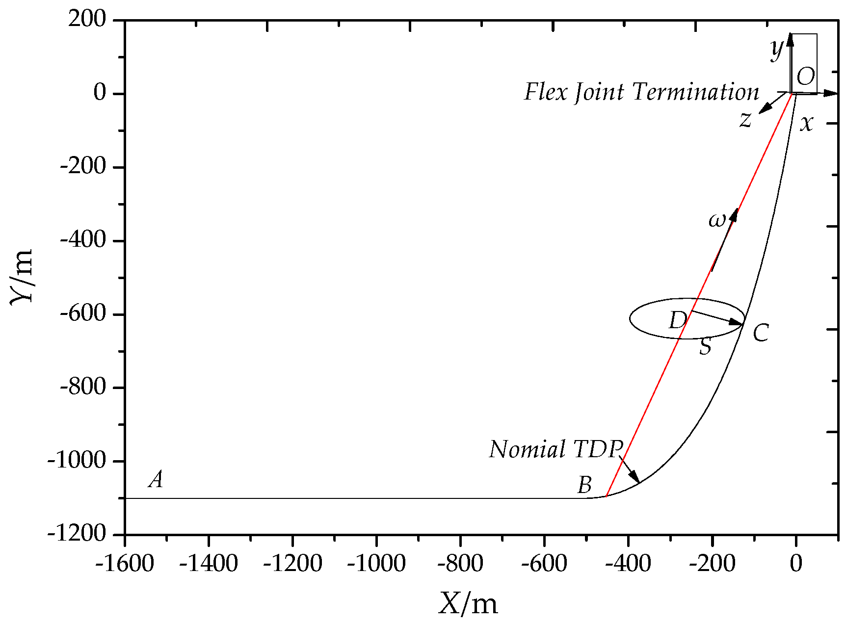
2.1. General Description of the Numerical Model

In this paper, a model consisting of a SCR large deflection slender beam module and a wave—load of suspension point in the z direction—rigid body swing module is developed. Based on Cable3D, the model can simulate wave loads, platform linear harmonic loads and SCR rigid body swing.

The Cable3D model [10] is developed to solve the complex response of steel catenary riser. Riser-platform, fluid-solid and pipe-soil interactions and the effect of rigid body swing are researched by the Cable3d software. The load model q as shown in Equation (4) is usually substituted by the subterm of SCR. These load subterms q integrated for the new complex phenomenon allow Cable3D to be further developed and extended. The integration model for simulation is shown in Figure 1. In this paper, a SCR large deflection slender beam model is adopted to solve the structure response. It is subjected to wave loads and loads in the z direction of the suspension point. The rigid body swing is simulated by using the SCR rigid body swing model.

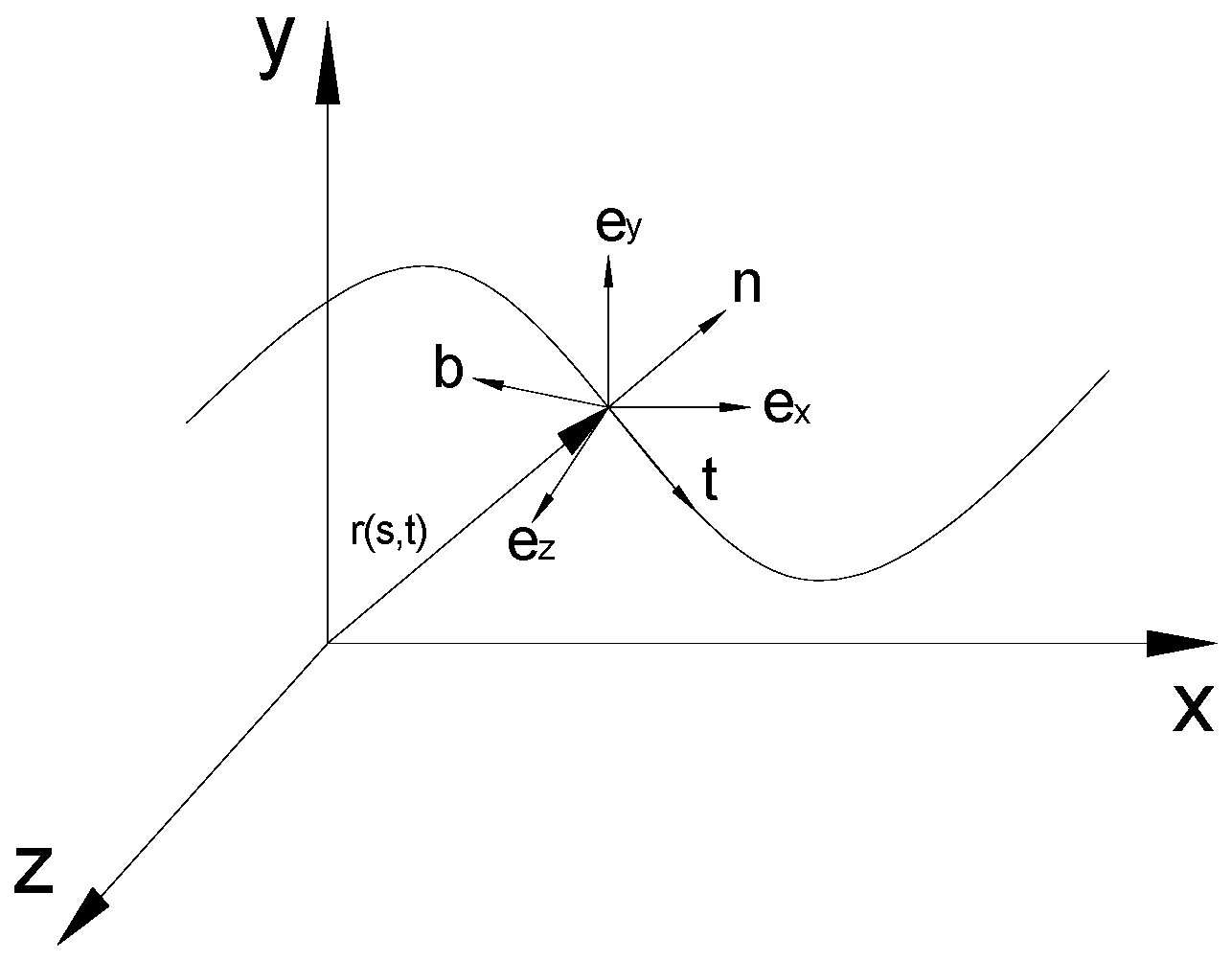
2.2. Basic Control Equation of SCR Motion

The basic governing equations [10] of the riser motion range from the beam balance equation to the riser vibration equation. In this process, the control equation is obtained from the expressions of load and mass terms. The basic theory of SCR provides a basic solving model for solutions. Then the wave, load of suspension point in the z direction and rigid body swing can be solved in the equation. The calculation of load such as rigid body swing usually has an iterative process. The following steps are detailed. Figure 2 shows the coordinate system of the riser. The shape of beam is represented by a vector S which is a function of the length r and time t.

According to the conservation, moment, linear and angular of momentum theorem, the equilibrium equation can be obtained:

$$\rho \frac{d^{2}r}{d{t}^2}(s,t)-q=\frac{dF}{ds}$$

(1)

$$\lambda \frac{dr}{ds}(s,t)-B\frac{d^{4}r}{d{s}^4}(s,t)=F$$

(2)

where F is the internal force of the beam section, q is the distributed external force per unit length on the beam, ρ is the mass of beam per unit length, λ is the Lagrangian operator and B is the beam bending stiffness.

After substituting the equation F’, the motion equation of the large-deflection slender beam is obtained. In this process, The Bernoulli-Euler theory is applied:

$$\rho \frac{d^{2}r}{d{t}^2}(s,t)=\lambda \frac{d^{2}r}{d{s}^2}(s,t)-B\frac{d^{4}r}{d{s}^4}(s,t)+q$$

(3)

After substituting the equation for the term q, the vibration control equation of the riser is obtained. In this process, the load calculation formula and vector transformation matrix are applied:

$$M\frac{d^{2}r}{d{t}^2}(s,t)=\lambda \frac{d^{2}r}{d{s}^2}(s,t)-B\frac{d^{4}r}{d{s}^4}(s,t)+q$$

(4)

where M is the mass matrix, B is the stiffness matrix, q is the load matrix and λ is the Lagrangian operator. The above formula is the basis of the structural numerical simulation. The mass, load and Lagrange operators of the structure form the basic solution and the basis model of SCR is composed of gravity, inertial force, drag force and F-K force.

2.3. SCR Rigid Body Rotation Submodel

The motion equation model of rigid body swing is established to simulate the phenomena of the steel catenary riser. Because the rigid body swing model cannot be directly simulated in commercial softwares, Cable3D is relatively superior to other commercial softwares in rigid motion simulations. The model adopts the theorem of momentum to study the moment balance of the riser. The response is solved through coupling the load term with the vibration equation. Then the result is obtained for the structural response of the rigid body swing in the rotation plane. The practical significance of the model is in providing a solution for the rigid body swing phenomenon. Figure 3 shows the rigid body swing system caused by loads such as deep water waves, flows and others. Figure 4 shows a real system of FMC Technologies. The rotation vector is represented by S which is a function of the node coordinates.

According to the moment of momentum theorem, the oscillating equation of rigid body swing is:

$$(m+m_a)s^2\frac{d^2{a}_r}{d{t}^2}+c_a{s}^2\frac{d{a}_r}{dt}=q_r$$

(5)

$$q_r=q_z\sqrt{s_1^2+s_2^2}+q_x{\omega }_2{s}_3-mg{\omega }_{1}s{a}_r$$

(6)

Substituting Equation (5) into Equation (4) and rearranging yields:

$$M\frac{d^{2}r}{d{t}^2}=\lambda \frac{d^{2}r}{d{s}^2}-B\frac{d^{4}r}{d{s}^4}+q_f+q_r+mg-(m+m_a)\frac{d^2{r}_r}{d{t}^2}-c_a\frac{d{r}_r}{dt}$$

(7)

$$M\frac{d^{2}r}{d{t}^2}=\lambda \frac{d^{2}r}{d{s}^2}-B\frac{d^{4}r}{d{s}^4}+q+mg-(m+m_a)\frac{d^2{r}_r}{d{t}^2}-c_a\frac{d{r}_r}{dt}$$

(8)

where m, m_a are the mass and additional mass per unit length of riser, c_a is the additional damping coefficient per unit length. q_x and q_z are the environmental load acting on per unit length. $a_r, {\dot{a}}_r,{\ddot{a}}_r$ are the angular displacement, angular velocity, angular acceleration of rigid body rotation, s₁, s₂ and s₃ are the projections of the radius S onto the axes x, y, z and ω₁, ω₂ and ω₃ are the projections of the vector onto the axes x, y, z.

It is expressed as the coordinate component form:

$$(m+m_a)(\frac{d^2{u}_b}{d{t}^2}+\frac{d^2{u}_r}{d{t}^2})+(c+c_a)\frac{d{u}_b}{dt}=q_x-c_a\frac{d{u}_r}{dt}-k{u}_b$$

(9)

$$(m+m_a)(\frac{d^2{v}_b}{d{t}^2}+\frac{d^2{v}_r}{d{t}^2})+(c+c_a)\frac{d{v}_b}{dt}=q_y-mg-c_a\frac{d{v}_r}{dt}-k{v}_b$$

(10)

$$(m+m_a)(\frac{d^2{w}_b}{d{t}^2}+\frac{d^2{w}_r}{d{t}^2})+(c+c_a)\frac{d{w}_b}{dt}=q_z-c_a\frac{d{w}_r}{dt}-k{w}_b$$

(11)

where $u_b,v_b,w_b,{\dot{u}}_b,{\dot{v}}_b,{\dot{w}}_b,{\ddot{u}}_b,{\ddot{v}}_b,{\ddot{w}}_b$ are the projection of displacement, velocity and acceleration on x, y, z and $u_r,v_r,w_r,{\dot{u}}_r,{\dot{v}}_r,{\dot{w}}_r,{\ddot{u}}_r,{\ddot{v}}_r,{\ddot{w}}_r$ are the projection of displacement, velocity and acceleration on of rigid body swing projected on x, y, z.

$${\overrightarrow{v}}_r={\dot{a}}_r(\overrightarrow{c}\times \overrightarrow{s}),{\overrightarrow{v}}_r={\dot{a}}_r(\overrightarrow{c}\times \overrightarrow{s}),{\overrightarrow{a}}_r={\ddot{a}}_r(\overrightarrow{c}\times \overrightarrow{s})$$

(12)

Expand it to the following expression:

$${\dot{u}}_r=\frac{d{a}_r}{dt}({\omega }_2{s}_3-{\omega }_3{s}_2),{\dot{v}}_r=\frac{d{a}_r}{dt}({\omega }_3{s}_1-{\omega }_1{s}_3){\dot{w}}_r=\frac{d{a}_r}{dt}({\omega }_1{s}_2-{\omega }_2{s}_1)$$

(13)

$${\ddot{u}}_r=\frac{d^2{a}_r}{d{t}^2}({\omega }_2{s}_3-{\omega }_3{s}_2){\ddot{v}}_r=\frac{d^2{a}_r}{d{t}^2}({\omega }_3{s}_1-{\omega }_1{s}_3){\ddot{w}}_r=\frac{d^2{a}_r}{d{t}^2}({\omega }_1{s}_2-{\omega }_2{s}_1)$$

(14)

2.4. SCR Wave Load Submodel

The wave load submodel is to solve the wave load equation in deep sea with riser moving relative to the water particle. The model uses Morison’s equation to study the relative load of the riser. The wave is calculated by a linear wave in deep water. The response of linear waves in deep water decreases as the depth increases. It is worth noting that this decreasing trend has a great influence on the trend of overall response. The loads such as waves and suspension point load in the z direction have the same trend.

Velocity potential is:

$${\phi }_0=\frac{gA}{\sigma }{e}^{kz}\sin (kx-\sigma t)$$

(15)

Horizontal velocity is:

$$u_x=A\sigma e^{kz}\cos \theta$$

(16)

Horizontal acceleration is:

$$\frac{\partial u_x}{\partial t}=A{\sigma }^2{e}^{kz}\sin \theta$$

(17)

In the wave model, the motion equation of SCR is:

$$f_H=\frac{1}{2}{C}_D\rho A(u_x-\dot{x})\left|u_x-\dot{x}\right|+C_M\rho \frac{\pi D^2}{4}\frac{\partial u_x}{\partial t}-C_m\rho \frac{\pi D^2}{4}\ddot{x}$$

(18)

where ${\varphi }_0$ is the velocity potential, u_x is the horizontal velocity of a water particle, ∂u_x/∂t is the horizontal acceleration, A is the wave amplitude, σ is the wave circular frequency, k is the wave number, ρ is the density, $\dot{x}$ is the velocity of the riser, D is the diameter, C_D is the drag force coefficient, C_M is the mass coefficient of mass and Cm is the additional mass coefficient.

2.5. SCR Load Submodel of Suspension Point in the z Direction

The main goal of load model in the z direction is to simulate the transverse load of the platform.

The top load in the z direction is:

$$F_z=k_{1}A\cos {\omega }_{s}t$$

(19)

Considering the interaction between waves and solids, the top load submodel is:

$$A_r=A-r$$

(20)

$$Q_z=k_1{A}_r^{}\cos {\omega }_{s}t$$

(21)

where A is the load amplitude, k₁ is the adjustment coefficient, usually 1, and ω_s is the load frequency.

The top load submodel is an equation to solve the simulation of cross flow direction load of platform. It is worth noting that the two loads appear perpendicular to each other in space, and as the wave load moves along the x direction, and the top load is in the z direction. Two harmonic load oscillations perpendicular to each other will form a stable elliptic curve if the frequencies are close to each other. If the frequency is expressed as an integer ratio, it is called Lissajous’ Figures [20,21].

Lissajous’ Figures provide theoretical support for analysis and verification of the load response perpendicular to each other. Equation (18) and Equation (5) can be substituted into Equation (4), and the control Equation (22) can be obtained:

$$M\frac{d^{2}r}{d{t}^2}=\lambda \frac{d^{2}r}{d{s}^2}-B\frac{d^{4}r}{d{s}^4}+q+mg-(m+m_a)\frac{d^2{r}_r}{d{t}^2}-c_a\frac{d{r}_r}{dt}+f_H+Q_z$$

(22)

where Q_z is the top load in the z direction. For Equation (22), the effect of load frequency on the equation is the frequency input on the right side. The load term is related to frequency, amplitude and phase. Then the input of different frequencies, amplitudes and phases makes the response complex and random.

2.6. Boundary Constraints and Iteration Conditions

According to the hypothesis that small deformations are allowed, the following formula is obtained:

$$\frac{dr}{dt}(s,t)\cdot \frac{dr}{dt}(s,t)={(1+\epsilon )}^2$$

(23)

The convergence criteria for the above solution is that the number of iterations is less than the allowed maximum number, or the difference between the two iterations is within the error range:

$$n>N_{\max }\mathrm{or}ep{s}_n<\left|\frac{r_n-r_{n-1}}{r_n}\right|$$

(24)

where n is the number of iterations, N_max is the allowed maximum number of iterations, and eps_n is the iterative error. Besides point A adopts an anchoring constraint, and the top suspension point O restrains the x and y directions. The load of the suspension point in the z direction (transverse flow direction) is added to the input file.

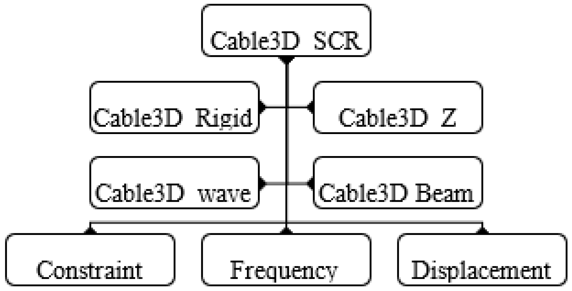
2.7. Summary of the Numerical Model

In this section, SCR and load numerical model are introduced. The SCR numerical model is a large deflection flexible beam model. The load numerical model introduces rigid body swing, load of suspension point in the z direction and wave model.

The Cable3D_Vswing program calculates the response under top load in the z direction, wave and rigid body swing. The difference between RT_CABLE [10] and Vswing is whether the top load in the z direction is considered or not. It is a key factor of the top load in the z direction for Vswing. The basic process mode of platform load includes the call of load function and the external input file.

This article adopts the method of external input file. Its biggest advantage is that it reduces the difficulty of load function fit. In addition, this paper promotes vector calculation from two-dimensional to three-dimensional, and this is a small improvement over the original RT_CABLE program.

3. The parameters and Verification for SCR Structure Simulation

The response of the SCR model in the cross-flow direction has been studied previously [10,11]. After the wave in the x direction and load of suspension point in the z direction are applied to the structure it appears that the loads are perpendicular to each other in space. The influence of response is worth studying after superposition of the rigid body swing.

The structure is affected by the mutually perpendicular load effect and rigid body swing. The response changes as the water depth increases and the influence of rigid body swing is of concern. Flow and fluid-solid coupling are not considered in this paper.

In this section, the Cable3D program and the Cable3D_Vswing program are respectively used for our simulation [11]. The Cable3D_Vswing program is a modified version of the load term Qforce. The coupled program improves the model of wave, load of suspension point in the z direction and rigid body swing. Cable3D calculates the structural response under the influence of wave load in the x direction and top suspension point load in the z direction. Cable3D_Vswing is used to calculate the response under the influence of waves, load of the suspension point in the z direction and rigid body swing. The difference is whether the influence of rigid body swing is considered in the response.

3.1. The Parameters of the SCR Structure

The density of crude oil in the riser is 865 kg/m³ and the density of sea water outside the pipe is 1025 kg/m³. The deep water linear wave is selected for calculation. The wave height is 3.5 m, period is 8.60 s, and the frequency is 0.11622 Hz. Petrobras Marlim, similar to the simulated structure, with a water depth of 1330 m, is connected to the undersea tree by pipelines. The development mode including SPAR, SCR and underwater tree is designed, with a SPAR draft of 153.169 m. It can accommodate eight top-tensioned risers. The SCR riser is suspended outside the soft cabin.

The design depth is 1100 m, the length of SCR is 2500 m, and the anchor point is 1800 m. The SCR adopts a five-layer structure from inside to outside. The different layers take corresponding roles respectively. The actual structure is exposed to dangerous conditions such as random response of the platform, waves and so on. In this paper, relatively simple conditions are selected for our simulation. The linear model is adopted for the seabed soil, without consideration of flow.

Table 1. Structure layers of the SCR bonded riser.

Structure	Function	Material	Density (kg/m3)
Bearing layer	Load bearing, etc.	API X-65	7850
Anticorrosive coating	Prevent osmotic corrosion	Epoxy resin	1440
Bonding layer	Interlayer bonding	Polypropylene	980
Thermal insulation layer	Cold oil not be transported	Foam Polypropylene	800
Protective layer	Prevent seabed damage, etc.	Polyethylene	900

shows the layers of the SCR bonded riser.

Table 2. Parameters of the SCR bearing layer [10].

Parameters	Value	Unit	Parameters	Value	Unit
The outer diameter	0.355	m	The moment of inertia	0.36123 × 10−3	m4
The inner diameter	0.305	m	The outer diameter area	0.99315 × 10−1	m2
Modulus elasticity	207.0	Gpa	The inner diameter area	0.72966 × 10−1	m2
Minimum yield strength	408.0	MPa	Unit length mass	0.2960	kg/m3
Poisson’s ratio	0.3	/	Unit length buoyancy	0.2137 4 × 104	N/m

lists the parameters of the bearing layer, and

Table 3. Parameters of the load of the suspension point in the z direction [11].

Cdt	Load	Direction	Amplitude/m	Frequency/Hz	Wave	ZDL	RBS
1	Cab1	Transverse flow	3.0	0.093	√	√
2	Cab 2	Transverse flow	2.0	0.101	√	√
3	Cab 3	Transverse flow	1.0	0.111	√	√
4	Csw1	Transverse flow	3.0	0.093	√	√	√
5	Csw 2	Transverse flow	2.0	0.101	√	√	√
6	Csw 3	Transverse flow	1.0	0.111	√	√	√

shows the top linear load parameters under different conditions.

RBS is a shortened form of Rigid Body Swing. ZDL is a shortened form of load of suspension point in the z direction. Four hundred 400 nodes, 399 beam elements and the three-time Hermite function are used to calculate the node response of SCR. The quadratic Hermite function is used to calculate different matrices. The matrices include the Lagrangian operator, mass, stiffness and external load matrix. The spring stiffness of the structural suspension point O and fixed point A is 0.1 × 10¹² Pa. The friction coefficient of the riser and seabed interaction is 0.2. The relaxation factor is 0.8 and the iteration error is 0.1 × 10⁻⁵. The number of iteration steps is 3600 and the calculation step is 0.1 s. Lift coefficient is 0.7, and drag force coefficient is 1.2. The mass coefficient is 1.0, and the hydrodynamic parameter is 0.355.

The wave load and the load of suspension point in the z direction make the structural response complex and random. Due to the action of water flow and waves, structural response of rigid body swing is complex and random. However, most finite element programs cannot directly calculate the rigid body swing. Therefore, in this paper the influence of rigid body swing is considered by a coefficient. The effect can be taken into account through multiplying the response under the main load by a coefficient.

In addition, the linear model is used for the load of suspension point in the z direction, which is suitable for better sea conditions, but not for worse ones. A linear model is adopted for waves, which is suitable for deep water, but not for inshore areas.

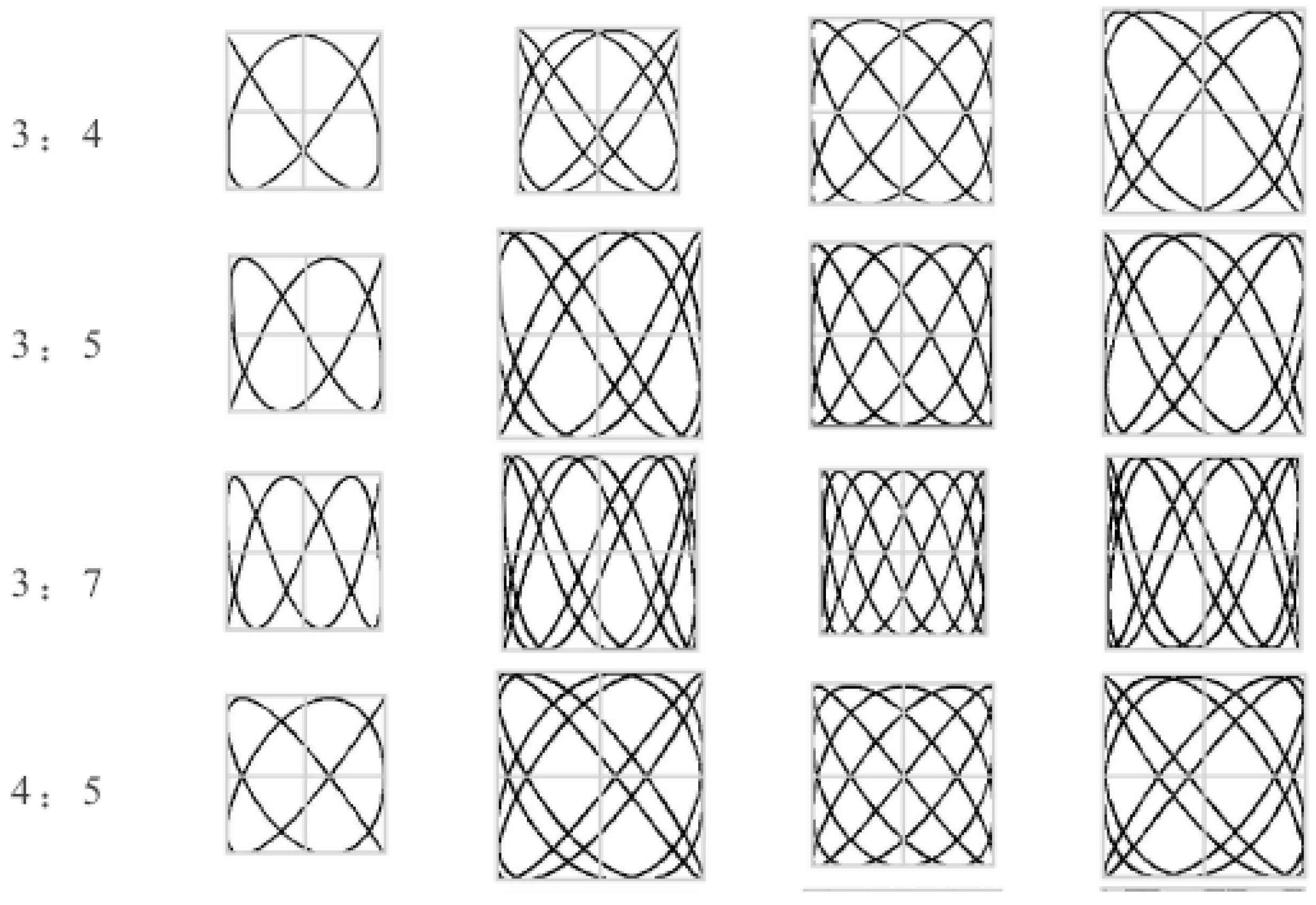
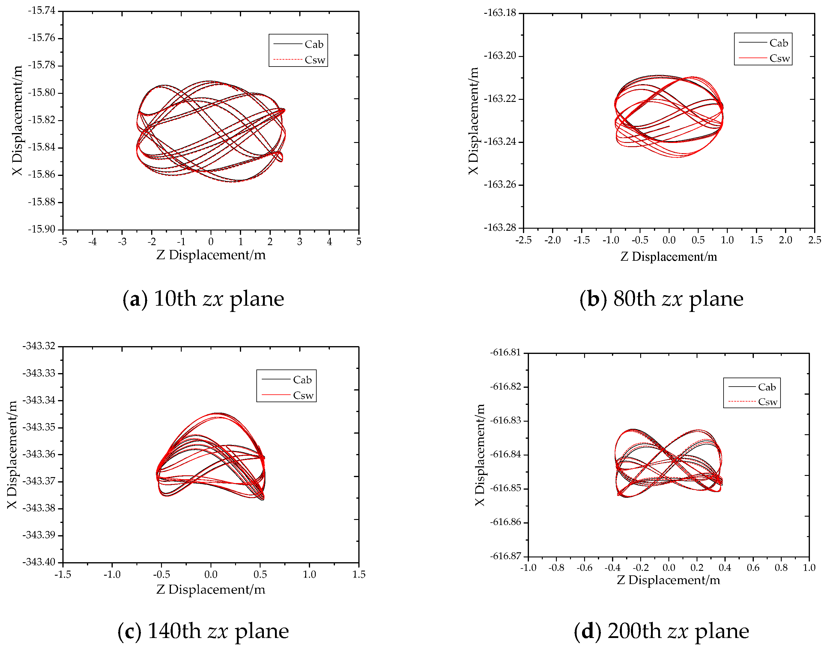
3.2. SCR Structural Lissajous Phenomenon and Verification

In real sea conditions, the load on the structure presents random characteristics and the response of random loads is shown in the perpendicular directions. This makes the response of the structure more intense or violent with random features, but there are also cases where the structure is subjected to simple loads. For example, the structure is subjected to waves, which adopt a deep water linear wave model, and the structure is also subjected to steady flow and the relatively stable movement of the platform, or if the structure is suspended on a fixed platform, the linear wave and steady flow in deep water models can be applied. In some of the above cases, the Lissajous phenomenon may also exist.

The Lissajous phenomenon of the SCR structure [20,21] is generated or defined by simple harmonic oscillations. The oscillations are perpendicular to each other. A stable curve will form when the frequency is close to the integral ratio. In this paper, the wave load is along the x direction and the load of the suspension point is in the z direction, so they are perpendicular to each other in space.

The response curve of the structure caused by wave load lacks check rules or standards. Then the Lissajous curve can play a certain auxiliary role in the verification. The check condition is that loads are perpendicular to each other, and the frequency ratio is integer ratio. The reference [20,21] can provide the curve to realize the verification:

$$x=A_1\cos (2\pi n_{1}t+{\varphi }_1) y=A_2\cos (2\pi n_{2}t+{\varphi }_2)$$

(25)

$$2\pi n_{1}t+{\varphi }_1+2k\pi =\pm \arccos \frac{x}{A_1} 2\pi n_{2}t+{\varphi }_2+2m\pi =\pm \arccos \frac{y}{A_2}$$

(26)

$\frac{n_1}{n_2}=\frac{m_1}{m_2}$ ($m_1$, $m_2$-prime numbers), and the trajectory equation is:

$$\cos (m_1\arccos \frac{y}{A_2}\pm m_2\arccos \frac{x}{A_1})=\cos (m_1{\varphi }_2-m_2{\varphi }_1)$$

(27)

The shape is determined by the amplitude ratio A₁/A₂, frequency ratio m₁/m₂ and cos(m₁ϕ₂ − m₂ϕ_1).

In this paper, the wave load frequency in the x direction is 0.11622 Hz and the load frequency of the suspension point in the z direction in the condition C1 is 0.093 Hz. After the data has been processed, the top load in the z direction is 0.09 Hz and the wave is 0.12 Hz. The common factor is 0.03, and the frequency ratio is 3:4.

From the viewpoint of load, the structure is subjected to the x direction wave load and the load of the suspension point in the z direction. The wave and the top load in the z direction are perpendicular to each other, and the frequency ratio ranges from 3:4 to 4:5. Then the wave and top load in the z direction can be simply checked and compared with the Lissajous curve.

For working condition 1, this paper adopts the Cable3D calculation results to compare with Lissajous’s figure. The z-x plane graphic response of the 10th–200th structure is studied. The structural response is shown in Figure 5. The response of 10th and 140th structure is similar to that of the second picture in 3:4 of Figure 6. The 80th and 200th response is similar to that of the fourth picture in 3:4 of Figure 6. These figures are also more similar to a 4:5 ratio.

On the whole, the structural response conforms to the basic characteristics of a Lissajous curve. The z-x plane response of the structure presents a zonal track characteristic. It is consistent with the characteristics of the Lissajous curve with high phase. From the 10th to 200th response, the zonal track decays gradually from a more complete distribution into a disordered one.

The amplitudes of the response in the x direction and z direction decrease with depth. The amplitude is positively correlated with the weakening of the wave and load of the suspension point in the z direction with increasing depth. The degree of deformation is strengthened or intense. The similarity degree of the graph and standard curve is also weakened. This represents an increase in the complexity of the bottom motion as the water depth increases. After the superimposition of rigid body swing, the basic features of the graph remain unchanged. The graph is shifted downward in the x axis and to the right in the z axis. From the above phenomenon, the calculation of the structure can be verified.

3.3. Structural Load Frequency Analysis and Verification

The response of a structure is usually a linear or nonlinear superposition of multiple load responses. Under the action of load, linear and nonlinear response curves are produced. The analysis of the load frequency can be helpful to the analysis of the main response. In this paper, the load frequency analysis is mainly to carry out with a FFT transformation which looks for the main frequency of the structure.

The solution method and data of load frequency are different for verification. Under load excitation, the frequency of the structure subjected to wave load in the x direction is 0.11622 Hz. Under the action of the load of suspension point in the z direction, the structure frequency is 0.093 Hz–0.111 Hz. The first frequency of bending vibration is solved by the Vandiver method to 0.016 Hz. The vibration frequency of the rigid body swing is solved by Rayleigh method to 0.029 Hz [11].

The Rayleigh method is shown in Equations (28)–(30):

$$T=\frac{1}{2}{\displaystyle \sum _i{m}_i{\dot{x}}_i^2}=\frac{1}{2}(\frac{1}{3}{m}_1{l}^2+\frac{1}{3}{m}_a{l}^2+m_2{l}^2){\omega }^2{A}^2{\cos }^2\theta$$

(28)

$$V=\frac{1}{2}{\displaystyle \sum _i{k}_i{x}_i^2}=\frac{1}{2}(k{l}^2)A^2{\sin }^2\theta =\frac{1}{2}(\frac{1}{2}{m}_{1}gl+\frac{1}{2}{m}_{a}gl+m_{2}gl)A^2{\sin }^2\theta$$

(29)

Because $T_{\max }=V_{\max }$, then the frequency can be derived:

$$\omega =\sqrt{\frac{1/2m_{1}gl+1/2m_{a}gl+m_{2}gl}{1/3m_1{l}^2+1/3m_a{l}^2+m_2{l}^2}}$$

(30)

Bending vibration method for solving natural vibration frequency is:

$$\omega ={(n\pi )}^2\sqrt{\frac{EI}{m{l}^4}},n=1,2,\cdots ,\infty$$

(31)

The response spectrum of the SCR structure is calculated by the FFT method and the response graphs of the amplitude and phase of the structure are obtained. In the previous FFT transformation, less attention is paid to the phase, which makes the analysis of the main frequency of structure inadequate. This paper will supplement some advice for these analyses. The numerical comparison of frequencies is as follows: wave frequency > load frequency of suspension point in the z direction > rigid body swing frequency > structure bending frequency (1st).

The frequency comparison can determine the relationship between the load frequency and the natural frequency and it can determine whether resonance is generated. These data can also provide theoretical values for comparison and verification of the FFT frequencies. In addition, the FFT amplitude corresponding to structural frequency can be used to analyze the influence of various loads. The main frequency of the structure, which is obtained from the phase curve, is shown in Section 4.4.2. The frequency of the FFT analysis is in good agreement with the results of theoretical formula.

Table 4. Load excitations of structure.

Frequency		Theory	FFT	Literature [11] 0.27 m/s	Literature [11] 0.30 m/s
WAVE (Hz)		0.11622	0.11600	/	/
ZDL (Hz)		0.09300	0.09299	/	/
RBS(Hz)		0.02900	0.02400	0.02800	0.02860
BV (Hz)	1st	0.01600	/	0.01550	0.01560
	2nd	0.06400	0.06800	/	/

compares structural results of formula, FFT and literature [11] methods.

RBS is the Rigid Body swing frequency and BV is the second-order frequency for Bending Vibration. ZDL is load frequency of the suspension point in the z direction. WAVE is the wave frequency.

3.4. The Summary of Verification

The verification of rigid body swing is very difficult. In the existing literature [11], there is an experimental method for verification. Due to its high cost and low effect of rigid body swing, it is sometimes difficult to capture the results satisfyingly. On the basis of the above, the z-x plane curve can be used for verification. Under the action of a specific frequency and amplitude, a curve can be formed to check by comparing the results with the Lissajous figures.

4. Response Analysis of the SCR Structure

4.1. General Description of Response

In the existing literature [22], response research mainly focuses on the relationship between amplitude and frequency. Among them, the amplitude mainly studies whether the structural response changes suddenly and whether the vibration amplitude exceeds the limit or not. Frequency mainly studies whether the load frequency generates resonance with the natural frequency.

The basic formula for the displacement solution [10] is:

$${\gamma }_{ikm}{M}_{njm}^{}{\ddot{u}}_{kj}^{}+{\alpha }_{ikm}{B}_m{u}_{kn}^{}+{\beta }_{ikm}{\tilde{\lambda }}_m^{}{u}_{kn}^{}={\mu }_{im}{q}_{mn}^{}+f_{in}^{}$$

(32)

The above formula is a set of equations for the model of a large deflection slender beam. It is a basic equation to solve static and dynamic displacementz. The SCR static displacement equation is a simplified version of Equation (32). The simplified formula is an expression of space, independent of time, which is the basis of the calculation.

The static basic equation of a steel catenary riser is:

$${\alpha }_{ikm}{B}_m{u}_{kn}+{\beta }_{ikm}{\tilde{\lambda }}_m{u}_{kn}={\mu }_{im}{q}_{mn}+f_{in}$$

(33)

where u is the displacement and $\tilde{\lambda }$ is the Lagrange operator.

The basic dynamic equation of a steel catenary riser is:

$${\gamma }_{ikm}{M}_{njm}^{(K)}{\ddot{u}}_{kj}^{(K)}+{\alpha }_{ikm}{B}_m{u}_{kn}^{(K)}+{\beta }_{ikm}{\tilde{\lambda }}_m^{(K)}{u}_{kn}^{(K)}={\mu }_{im}{q}_{mn}^{(K)}+f_{in}^{(K)}$$

(34)

The initial displacement, velocity, acceleration and Lagrange operator can be obtained by the static Equation (33). $M^{(K)}$ and $q^{(K)}$ can be obtained from the above Equation (34). The SCR displacement response calculation is based on the above solution.

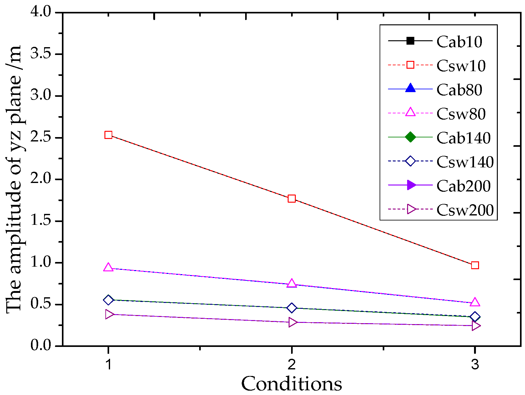
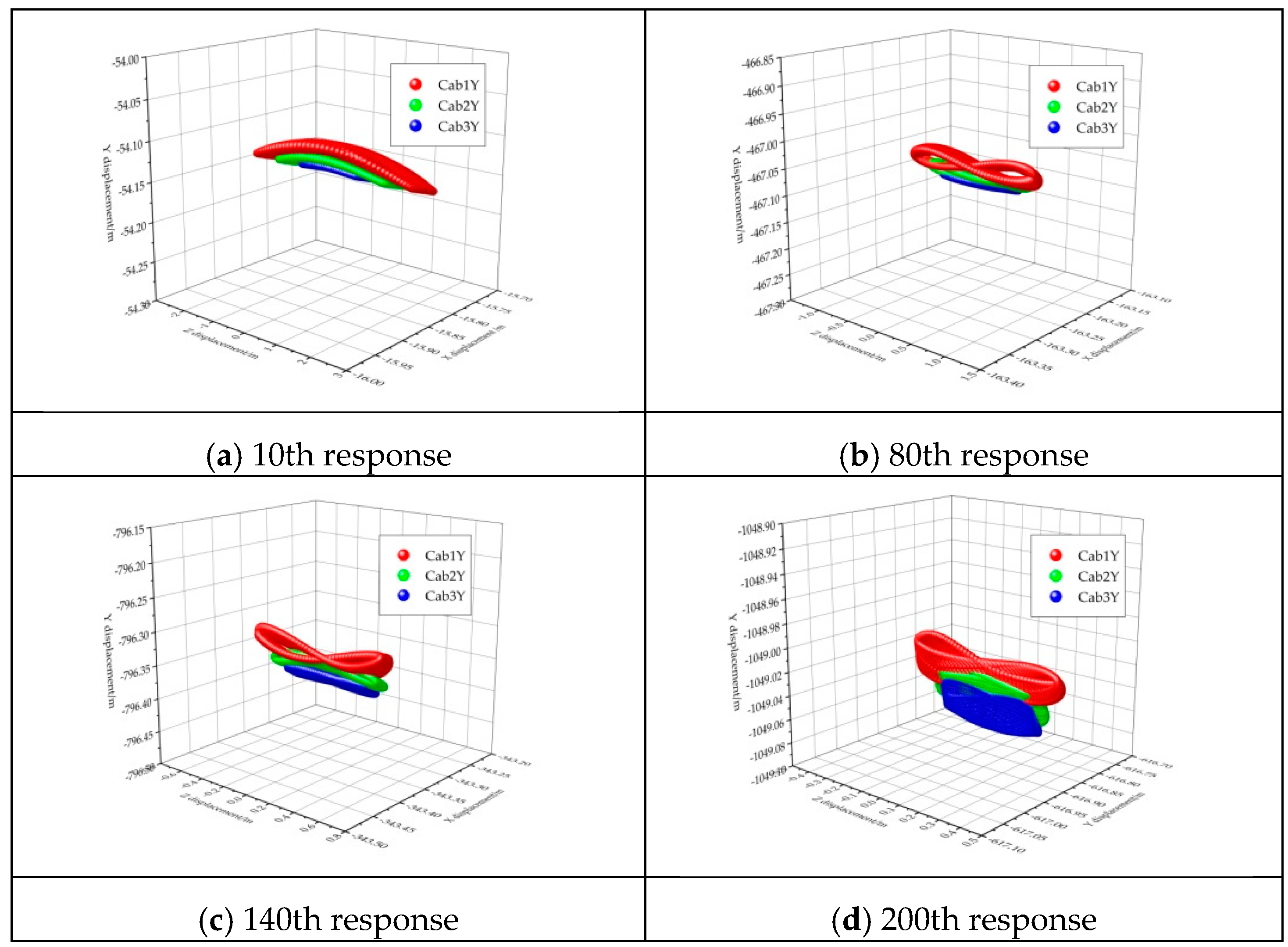
4.2. SCR Three-Dimensional and Two-Dimensional Response Analysis

In this paper, SCR response analysis is carried out from three-dimensional analysis to one-dimensional analysis. The response characteristics of structural space are the main contents or emphases of this paper. The process from three dimensions to one represents the feature from integral, plane to one dimension. Under the action of wave and rigid body swing, the effect of load of suspension point in the z direction on structure has been studied. Figure 7 and

Table 5. The location of nodes.

	X/m	Y/m
10	−15.8273	−54.1376
80	−163.2674	−467.0530
140	−343.3629	−796.3470
200	−616.8364	−1049.0293

show the static location of different nodes.

The responses of the 10th, 80th, 140th and 200th nodes of the structure can be obtained. The three-dimensional figure without rigid body swing is obtained as shown in Figure 8 and the y-z plane diagram with and without rigid body swing is shown in Figure 9.

The vertical coordinate is the y-axis which is connected to the z-axis, and the x-axis is perpendicular to the y-z plane in Figure 8, which shows the three-dimensional response of non-rigid body swing under wave and load of suspension point in the z direction. Figure 9 shows a figure with or without rigid body swing in the y-z plane.

There is no obvious difference in shape or overall pattern between the two groups. This indicates that the influence of rigid body swing is weak. The y-z plane is a projection in the y (swaying or vertical) and z (cross-flow) plane of the structure. There is no significant difference in the plane of vertical and cross flow direction (the rigid body swing plane). This means that when the structure is subjected to the load of the suspension point in the z direction there is no significant difference in the rotation plane. The influence of rigid body swing on the plane is weak. This point can be understood from the amplitude of rigid body swing and top load in the z direction. The top load in the z direction is applied by 3 m (platform response) with significant amplitude relative to the rigid body swing.

The time curve in the z direction is expressed graphically and gradually in the following Section 4.3. Under different conditions, the vibration decreases gradually in the transverse direction, however, it increases gradually in the vertical depth. The oscillation with a graphics like eight in the plane gradually decreases.

In terms of the responses of different nodes, the response of the y-z plane becomes more complicated as the node number increases. The overall response is that the 10th’s y-z plane oscillation gradually develops into the 200th’s z-x plane oscillation. There is also a rotation around the z axis to the z-x plane. The swing mode: 10th’s vibration is a narrow amplitude oscillation in the y-z plane. The 80th vibration is a wide amplitude oscillation with a graphic form shaped like eight. The 140th vibration is relatively narrow range oscillation in the y-z plane with an eight-like graph. Tthere is a rotation around the z-x axis. The 200th vibration is a narrow range oscillation in the y-z plane with a graph like an eight. There is also a rotation around the z axis, and z-x plane gradually oscillates with a graph like an eight.

The amplitude of the swing gradually decreases. The maximum deviations from the center of movement of the 10th, 80th, 140th and 200th node gradually decrease. The structural response also decreases after the superposition of rigid body swing in condition 1 and the rigid body swing decreases the motion of the structure in the y-z plane. For condition 2 and 3, the maximum influence of rigid body swing is 1.95% for the 140th node. The difference and amplitude are shown in

Table 6. Amplitude and difference of yz plane swing in different conditions.

Cdt	Node	Cab (m)	Csw (m)	Diff
1	10th	2.53294	2.53254	−0.016%
1	80th	0.93671	0.93484	−0.200%
1	140th	0.55687	0.55431	−0.460%
1	200th	0.38464	0.38395	−0.179%
2	10th	1.76859	1.76816	−0.024%
2	80th	0.74119	0.74525	0.548%
2	140th	0.45918	0.45993	0.163%
2	200th	0.28813	0.28781	−0.111%
3	10th	0.97038	0.97032	−0.006%
3	80th	0.51709	0.51871	0.313%
3	140th	0.35021	0.35704	1.950%
3	200th	0.24737	0.24684	−0.214%

below.

The motion of the structure in the y-z plane presents a complicated state with the increase of water depth. The amplitude of oscillation attenuation of the top node is the greatest. The activity is the most intense near the top suspension point region of the 10th–80th nodes. As the water depth or the condition increases, the amplitude decreases, as shown in Figure 10 and Figure 11. The figures help to understand the response from a three-dimensional perspective.

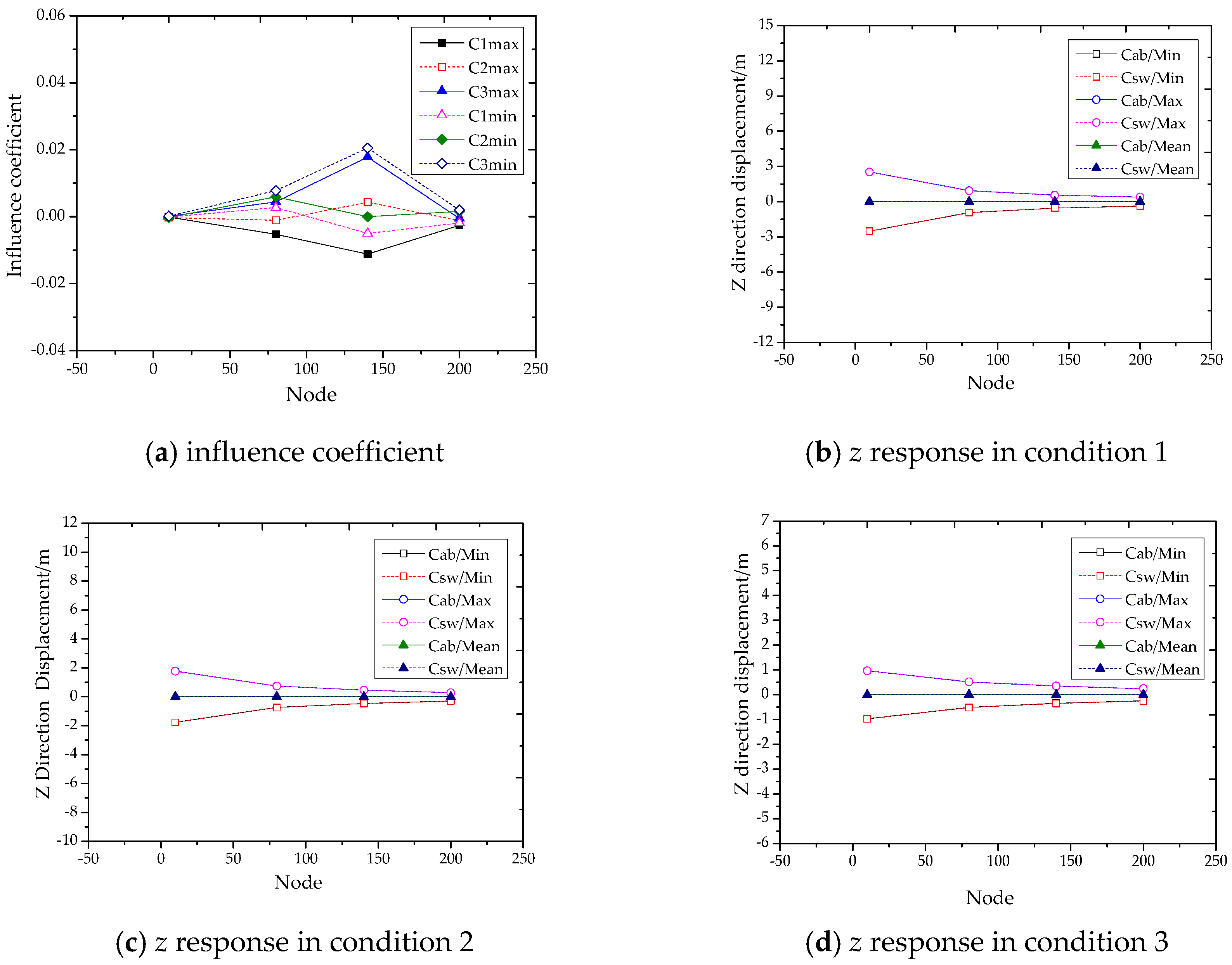
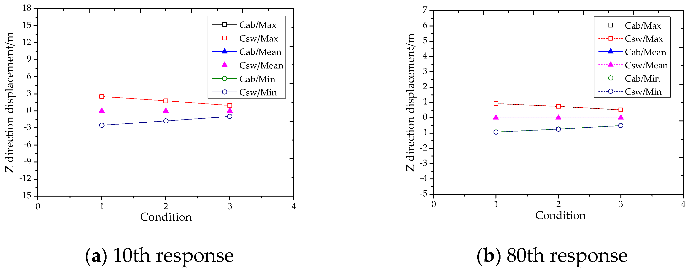
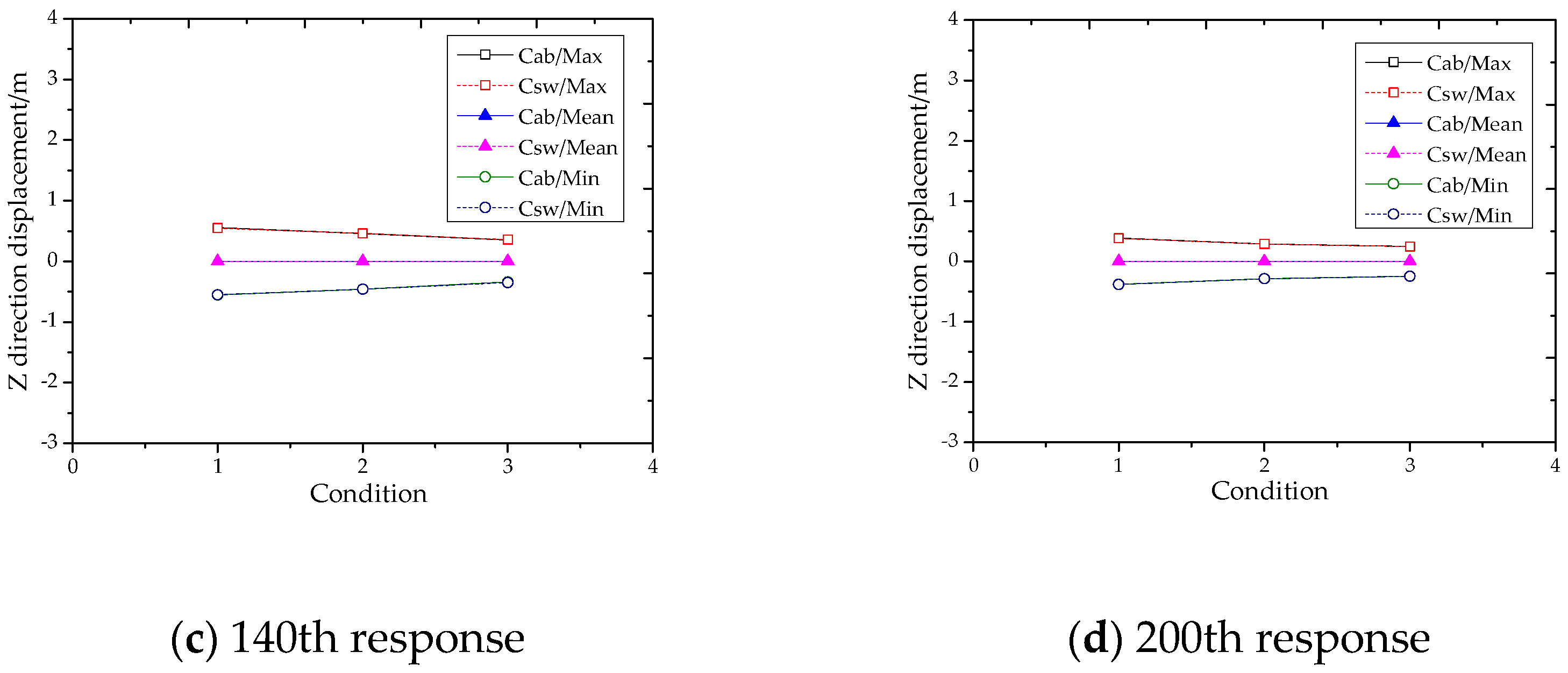
4.3. Analysis of the z-Direction Response of the SCR Structure

4.3.1. SCR Response Analysis

For SCR, the above response characteristics in the y-z plane are the response characteristics of a rigid body swing plane. The calculation in the z direction is from an angle perpendicular to the x-y plane (riser bending plane). It is an indispensable part of the three-dimensional motion response. Its calculation is very important for the vibration system.

The calculation of the cross-flow response of thestructure includes VIV, cross-flow load, rigid body swing and so on. There are plenty of studies on structures with bending vibrations and vortex-induced vibrations, while the response research of the rigid body swing in the cross-flow direction is relatively less common. The responses of the 10th, 80th, 140th and 200th nodes in condition 1 are shown in Figure 12. The formula of the coefficients is as follows:

$$R_{cab}=R_{wave}+R_z R_{csw}=R_{wave}+R_z+R_{rbs}$$

(35)

$$Inc=(R_{csw}-R_{cab})/R_{cab}$$

(36)

$$Rdt=\{\begin{array}{c}(R_n-R_{next})/R_{10th},n=10th,80th,140th\\ (R_{200th}-0)/R_{10th},n=200th.\end{array}$$

(37)

where R_cab is the structural response under waves and the load of the suspension point in the z direction, R_csw is the structural response under the action of waves, top load in the z direction and rigid body swing, R_wavew is the structural response under wave action, R_rbs is the structural response under rigid body swing, R_z is the structural response under the top load in the z direction, Inc is the growth rate and Rdt the relative reduction.

Figure 12 shows the results of condition 1. The overall response of the structure is observed by selecting four nodes. A linear harmonic load from the z direction is imposed on the structure. The cross-flow extreme, balance position and standard deviation are shown in Table 6 and

Table 7. Maximum, minimum and increase of node response.

Cdt	Node	Cabmax (m)	Cswmax (m)	Incmax	Cabmin (m)	Cswmin (m)	Incmin
1	10th	2.53031	2.52998	−0.01%	−2.52323	−2.52298	−0.01%
1	80th	0.93399	0.92900	−0.53%	−0.93500	−0.93754	0.27%
1	140th	0.55306	0.54688	−1.12%	−0.55430	−0.55152	−0.50%
1	200th	0.38398	0.38300	−0.26%	−0.38312	−0.38239	−0.19%
2	10th	1.76981	1.76936	−0.03%	−1.76465	−1.76436	−0.02%
2	80th	0.74551	0.74471	−0.11%	−0.73664	−0.74101	0.59%
2	140th	0.45820	0.46017	0.43%	−0.45952	−0.45950	0.00%
2	200th	0.28697	0.28663	−0.12%	−0.28717	−0.28764	0.16%
3	10th	0.96836	0.96843	0.01%	−0.96587	−0.96594	0.01%
3	80th	0.51933	0.52159	0.44%	−0.50926	−0.51324	0.78%
3	140th	0.35072	0.35698	1.78%	−0.34172	−0.34872	2.05%
3	200th	0.24683	0.24670	−0.05%	−0.24590	−0.24638	0.20%

. They are on behalf of the vibration amplitude and intensity. This shows that the cross-flow maximum of structure decreases with depth under wave action and load of the suspension point in the z direction. The minimum value and standard deviation of the structural vibration are also decreasing. The main reason is that the wave velocity, etc. decreases with depth. As the water depth increases, the response of other particles produced by the top z-direction excitation decreases, therefore, the wave and top load in the z direction weaken the structural response.

Under the action of waves, load of the suspension point in the z direction and rigid body swing, the conclusion is similar to that of non-rigid body swing. The cross-flow response of condition 1 is shown in Table 7 and

Table 8. Equilibrium and standard deviation of node response.

Cdt	Node	Cabmean (m)	Cswmean (m)	Cabstd (m)	Cswstd (m)
1	10th	0.00315	0.00315	1.71816	1.71816
1	80th	−0.00238	−0.00238	0.62457	0.62443
1	140th	0.00111	0.00112	0.37026	0.37051
1	200th	0.00144	0.00149	0.25996	0.25951
2	10th	1.00 × 10−4	9.87 × 10−5	1.1907	1.19067
2	80th	6.71 × 10−4	6.68 × 10−4	0.49967	0.4997
2	140th	5.90 × 10−4	5.86 × 10−4	0.31063	0.31095
2	200th	4.23 × 10−4	4.29 × 10−4	0.19729	0.19767
3	10th	4.77 × 10−4	4.72 × 10−4	0.63321	0.63322
3	80th	4.28 × 10−4	3.98 × 10−4	0.34035	0.34057
3	140th	4.75 × 10−4	4.23 × 10−4	0.23391	0.23431
3	200th	4.34 × 10−4	3.81 × 10−4	0.17002	0.16968

. As the depth increases, the cross-flow response decreases under the wave, top load in the z direction and rigid body swing influence. After superimposition of rigid body swing, the response’s trend is similar to that under the action of waves and the top load in the z direction only. Then the structure is relatively weakly affected by rigid body swing.

The rigid body swing, wave and top action are considered as simply a linear superposition. The maximum growth rates of 10th–200th nodes are −0.01%, −0.53%, −1.12% and −0.26%, respectively, as shown in Table 7 and Table 8. By comparing condition 2 and 3, there is maximum superposition of 1.78%. The response of the touch down point and suspension point are weakened under the rigid body swing. For the 140th node the influence of vibration is in a range of −1.5% to 2.0%.

Vibration in a certain range represents the phase difference between wave, linear load of the suspension point in the z direction and rigid body swing. However, the effect of rigid body swing first increases and then decreases with depth. It is positively correlated to vector S. The rest of the conditions are similar, as shown in Table 7 and Table 8.

Figure 13 shows the variation of the 10th–200th nodes with different conditions. The results show the response of structure decreases when the amplitude of the top load in the z direction decreases. With the increase of water depth, the displacement of each node decreases relative to the response of the top node. The attenuation of the 10th–80th nodes is more intense, and the attenuation is weaker after the 80th, as shown in

Table 9. Reduction, difference and normalized values of node’s maximum response.

Cdt	Node	Cabmax (m)	Cswmax (m)	Rdtcab	Rdtcsw	Diff	Nmlcab	Nmlcsw
1	10th	2.52716	2.52683	62.95%	63.14%	0.19%	1.00	1.00
1	80th	0.93637	0.93138	15.21%	15.26%	0.05%	1.00	1.00
1	140th	0.55195	0.54576	6.70%	6.50%	−0.20%	1.00	1.00
1	200th	0.38254	0.38151	15.14%	15.10%	−0.04%	1.00	1.00
2	10th	1.76971	1.76926	57.91%	57.95%	0.04%	0.70	0.70
2	80th	0.74484	0.74404	16.23%	16.08%	−0.15%	0.79	0.79
2	140th	0.45761	0.45958	9.67%	9.80%	0.13%	0.83	0.83
2	200th	0.28655	0.28620	16.19%	16.18%	−0.01%	0.75	0.75
3	10th	0.96788	0.96796	46.39%	46.16%	−0.23%	0.38	0.38
3	80th	0.51890	0.52119	17.42%	17.01%	−0.41%	0.55	0.55
3	140th	0.35025	0.35656	10.73%	11.39%	0.66%	0.62	0.63
3	200th	0.24640	0.24632	25.46%	25.45%	−0.01%	0.64	0.64

and

Table 10. Reduction, difference and normalized values of node’s minimum response.

Cdt	Node	Cabmin (m)	Cswmin (m)	Rdtcab	Rdtcsw	Diff	Nmlcab	Nmlcsw
1	10th	−2.52323	−2.52298	62.94%	62.84%	−0.10%	1.00	1.00
1	80th	−0.9350	−0.93754	15.09%	15.30%	0.21%	1.00	1.00
1	140th	−0.5543	−0.55152	6.78%	6.70%	−0.08%	1.00	1.00
1	200th	−0.38312	−0.38239	15.18%	15.16%	−0.03%	1.00	1.00
2	10th	−1.76465	−1.76436	58.26%	58.00%	−0.25%	0.70	0.70
2	80th	−0.73664	−0.74101	15.70%	15.96%	0.25%	0.79	0.79
2	140th	−0.45952	−0.45950	9.77%	9.74%	−0.03%	0.83	0.83
2	200th	−0.28717	−0.28764	16.27%	16.30%	0.03%	0.75	0.75
3	10th	−0.96587	−0.96594	47.27%	46.87%	−0.41%	0.38	0.38
3	80th	−0.50926	−0.51324	17.35%	17.03%	−0.31%	0.54	0.55
3	140th	−0.34172	−0.34872	9.92%	10.59%	0.67%	0.62	0.63
3	200th	−0.24590	−0.24638	25.46%	25.51%	0.05%	0.64	0.64

.

The influence coefficient ranges from −0.02 to 0.02, as shown in Figure 14a. The influences of rigid body swing on different extreme conditions are statistically analyzed. The maximum is 0.66% at the 140th node. To some extent, if the rigid body swing cannot be calculated, it is appropriate to use a response times 1.02 for the effect of rigid body swing. Figure 14b–d show that with the increase of nodes in each condition, the top region displays the maximum response and the displacement gradually weakens for conditions 1–3. This trend is similar to the change trend of wave loads. The oscillation of the load of suspension point in the z direction decreases with the depth of the water. Tthe pendulum of Equation (8) can explain the trend in a simple way. This tendency of decrease with depth can also be used as part of the verification for calculations.

The normalization value of Table 9 and Table 10 can directly obtain the response coefficient of each condition relative to condition 1. This coefficient can explain why the response variation is more influenced by condition amplitude. The structural response decreases by 20–30% when the amplitude of structural condition decreases by 50%.

4.3.2. Response Analysis of the Top Suspension Point of the SCR Structure

The top suspension point of the SCR has a larger response amplitude in this paper. It belongs to the structural danger area, which should be studied further [22]. The 10th node presents the Lissajous phenomenon in the z-x plane when the frequency ratio is 3:4 in Figure 6. Figure 8 and Figure 9 show that the oscillation in the y-z plane is in a narrow range. The maximum fluctuation standard deviation and reduction with the depth is shown in Table 9 and Table 10. The reason is that there is a maximum of wave and top load in the z direction in the top suspension point area. In addition, the response decreases fastest in that region, then it becomes more dangerous.

On the above basis, this paper carried out the spectral analysis, and the results are shown in

Table 11. Spectrum analysis of node 10.

C	Node	X (Hz)	Cab/Y (m2·s)	Csw/Y (m2·s)
1	10th	0.092991	1.710155	1.710178
2	10th	0.100990	1.676353	1.676343
3	10th	0.110989	0.885023	0.885041

and Figure 15. The response presents a unimodal state. The spectral peak corresponds to load frequency of suspension point in the z direction. The structural response presents a forced motion. As the frequency increases, the spectral peak of the structure decreases. The main reason is that the amplitude of the motion is decreasing. The spectral peak has increased in condition 1. However, it decreases in condition 2–3 after superimposition of the rigid body swing, as shown in Table 11.

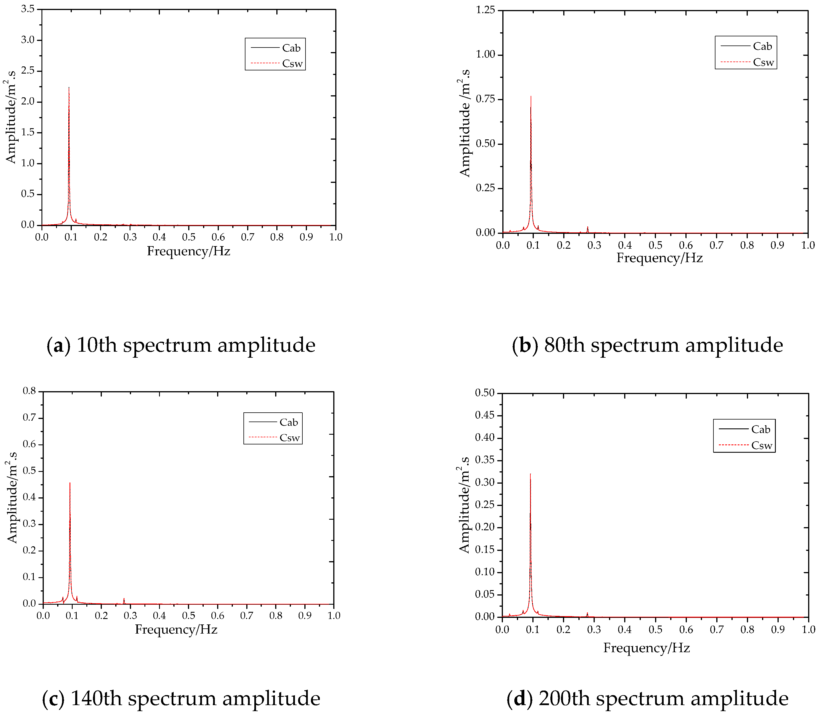
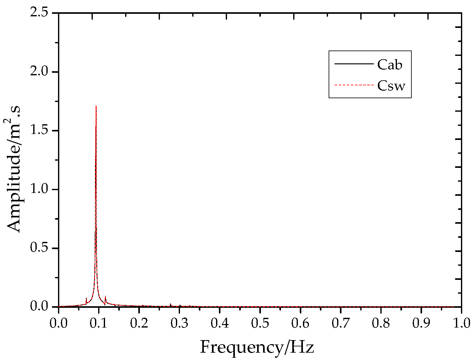
4.4. Spectral Analysis

4.4.1. Basic Theory of FFT Calculation

FFT [11] is a transformation from the response signal with time to the response signal with frequency. FFT is also used to calculate the spectral curve of the structure in this paper. In this process, the main frequency and influence frequency can be obtained by the spectral analysis. In addition, the response of the structure includes amplitude and phase. The main frequency and the influence frequency can be obtained by the amplitude curve of the structure. They can also be obtained by the phase curve of the structure. In this paper, the phase curve is more accurate to obtain them:

$$F_n={\displaystyle \sum _{i=0}^{N-1}{x}_i{e}^{\frac{-2\pi j}{N}Ni}}$$

(38)

$$Phase=atc\tan (I_m/R_e)$$

(39)

$$Amplitude=\{\begin{array}{c}\sqrt{R_e^2+I_m^2}/n,i=0,n/2\\ 2\ast \sqrt{R_e^2+I_m^2}/n,other\end{array}$$

(40)

where F_n is the discrete transform (DFT), N is the calculated length and x_i is the sequence. The phase and amplitude of the single side spectrum ($i$ = 0 − $n/2$) are shown in the formula. The window function is calculated by rectangle. Spectrum analysis is rearranged to reduce leakage and the normalization method of the spectral density is the Mean Square Amplitude (MSA) method.

4.4.2. Analysis of Structural Main Frequency and the Influence Frequency

The frequency of the structure can be obtained by spectral analysis. The variation of the main frequency with water depth is studied. The influences of rigid body swing and the load of the suspension point in the z direction on the main frequency are analyzed. The main frequency is the dotted line position of the amplitude-phase diagram for the 10th-200th nodes in Figure 16. RBS is a shortened form of the rigid body swing. BV is a shortened form of the bending vibration. ZDL is a shortened form of the top load in the z direction. WAVE is a shortened form of wave action. These frequencies have been expressed in Section 3.2.

The amplitude frequency curve of the structural response is difficult to resolve due to the small impact. However, good resolution is obtained in the phase frequency curve. This can be used to judge and check the influence frequency. From the amplitude and phase curve of the structure, the main frequency of the structure is the load frequency of the suspension point in the z direction. The main frequency shows a cliff-edge or rapid change of the phase on the phase curve, but it turns into a peak on the amplitude curve.

Structural frequencies and amplitudes are shown in

Table 12. Structural frequencies and amplitudes of different loads.

Node	Cdt	RBS	RBS	BV	BV	ZDL	ZDL	WAVE	WAVE
		X (Hz)	Y (m2·s)	X (Hz)	Y (m2·s)	X (Hz)	Y (m2·s)	X (Hz)	Y (m2·s)
10th	Cab	0.024	0.011804	0.0681	0.021044	0.0921	2.238628	0.1161	0.107761
	Csw	0.024	0.012534	0.0681	0.020742	0.0921	2.223184	0.1161	0.105901
80th	Cab	0.024	0.016019	0.0680	0.035739	0.0920	0.770012	0.1160	0.041897
	Csw	0.024	0.016045	0.0681	0.035919	0.0921	0.769957	0.1161	0.038988
140th	Cab	0.024	0.005458	0.0681	0.027404	0.0920	0.457074	0.1161	0.025370
	Csw	0.024	0.005445	0.0681	0.027346	0.0920	0.457155	0.1161	0.029915
200th	Cab	0.024	0.007584	0.0680	0.015419	0.0920	0.320702	0.1160	0.013523
	Csw	0.024	0.007606	0.0680	0.015786	0.0920	0.320106	0.1160	0.014074
Theory		0.0290	/	0.0640	/	0.0930	/	0.1162

and

Table 13. Percentage relative to total frequency’s amplitude of different loads.

Node	Cdt	RBS	BV	ZDL	WAVE
10th	Cab	0.496%	0.884%	94.090%	4.529%
	Csw	0.531%	0.878%	94.109%	4.483%
80th	Cab	1.855%	4.138%	89.156%	4.851%
	Csw	1.864%	4.172%	89.435%	4.529%
140th	Cab	1.059%	5.318%	88.700%	4.923%
	Csw	1.047%	5.260%	87.938%	5.754%
200th	Cab	2.123%	4.316%	89.775%	3.786%
	Csw	2.127%	4.415%	89.522%	3.936%

. The FFT calculation frequency is close to the theoretical value. The importance of load can be obtained from a percentage comparison relative to the total frequency’s amplitude, as shown in Table 13. From the top to the bottom, the bending vibration and waves have limited effects on the frequency. Rigid body swing has little effect on the frequency and increases with water depth, as shown in Table 13.

4.4.3. Analysis of the Structural Main Frequency

The frequency response of the 10th–200th nodes in Figure 17 is obtained through the spectrum analysis of condition 1.

Table 14. Main frequency and reduction of with/no rigid body swing along water depth.

Cdt	Node	Cabx (Hz)	Caby (m2·s)	Cswx (Hz)	Cswy (m2·s)	Cabrdt	Cswrdt	Diffrdt
1	10th	0.092991	2.238628	0.092991	2.223184	65.60%	65.37%	−0.24%
1	80th	0.092991	0.770012	0.092991	0.769957	13.98%	14.07%	0.09%
1	140th	0.092991	0.457074	0.092991	0.457155	6.09%	6.16%	0.07%
1	200th	0.092991	0.320702	0.092991	0.320106	14.33%	14.40%	0.07%
2	10th	0.100990	1.209967	0.100990	1.209961	62.08%	62.09%	0.01%
2	80th	0.100990	0.458852	0.100990	0.458673	11.75%	11.73%	−0.02%
2	140th	0.100990	0.316691	0.100990	0.316708	9.46%	9.43%	−0.03%
2	200th	0.100990	0.202235	0.100990	0.202626	16.71%	16.75%	0.03%
3	10th	0.110989	0.597511	0.110989	0.597504	46.20%	46.24%	0.04%
3	80th	0.110989	0.321454	0.110989	0.321218	16.88%	16.87%	−0.01%
3	140th	0.110989	0.220580	0.110989	0.220394	10.02%	10.04%	0.03%
3	200th	0.110989	0.160731	0.110989	0.160395	26.90%	26.84%	−0.06%

and

Table 15. Difference and normalized values of spectrum.

Cdt	Node	X (Hz)	Caby (m2·s)	Cswy (m2·s)	Diff	Cabnml	Cswnml
1	10th	0.092991	2.238628	2.223184	−0.69%	1.00	1.00
2	10th	0.100990	1.209967	1.209961	0.00%	0.54	0.54
3	10th	0.110989	0.597511	0.597504	0.00%	0.27	0.27
1	80th	0.092991	0.770012	0.769957	−0.01%	1.00	1.00
2	80th	0.100990	0.458852	0.458673	−0.04%	0.60	0.60
3	80th	0.110989	0.321454	0.321218	−0.07%	0.42	0.42
1	140th	0.092991	0.457074	0.457155	0.02%	1.00	1.00
2	140th	0.100990	0.316691	0.316708	0.01%	0.69	0.69
3	140th	0.110989	0.22058	0.220394	−0.08%	0.48	0.48
1	200th	0.092991	0.320702	0.320106	−0.19%	1.00	1.00
2	200th	0.100990	0.202235	0.202626	0.19%	0.63	0.63
3	200th	0.110989	0.160731	0.160395	−0.21%	0.50	0.50

are the main frequency of the structure in different conditions. In terms of the main frequency, the x values are 0.092991 Hz, 0.100990 Hz and 0.110989 Hz. The numerical value is close to the load frequency of the suspension point in the z direction of the structure. The frequency of the external load is the same as the response frequency, which is a forced motion. After the superposition of rigid body swing, the main frequency of the structure is still same. It means that the rigid body swing has no obvious influence on the main frequency.

From the main frequency amplitude of the structure, the Y value (spectral amplitude) is studied. The spectral amplitude decreases as the node number increases. The maximum reduction is 40–60% in the top area, as shown in Table 14. As the water depth increases, it decreases first and then increases after reaching the minimum value at the 140th node. The effect does not change significantly after superimposition of rigid body swing. After superimposition of rigid body swing, the maximum impact is about −0.2% in bottom area, as shown in Table 15. At the 140th node, main frequency decreases the least with depth. The rigid body swing makes the main frequency amplitude of structure increase slightly. Then the main frequency amplitude of the structure is normalized. The amplitude of structure decreases gradually with the conditions, as shown in Table 15. The main frequency amplitude represents the energy of the response of the structure. The main frequency is strongly affected by the decrease of amplitude of conditions.

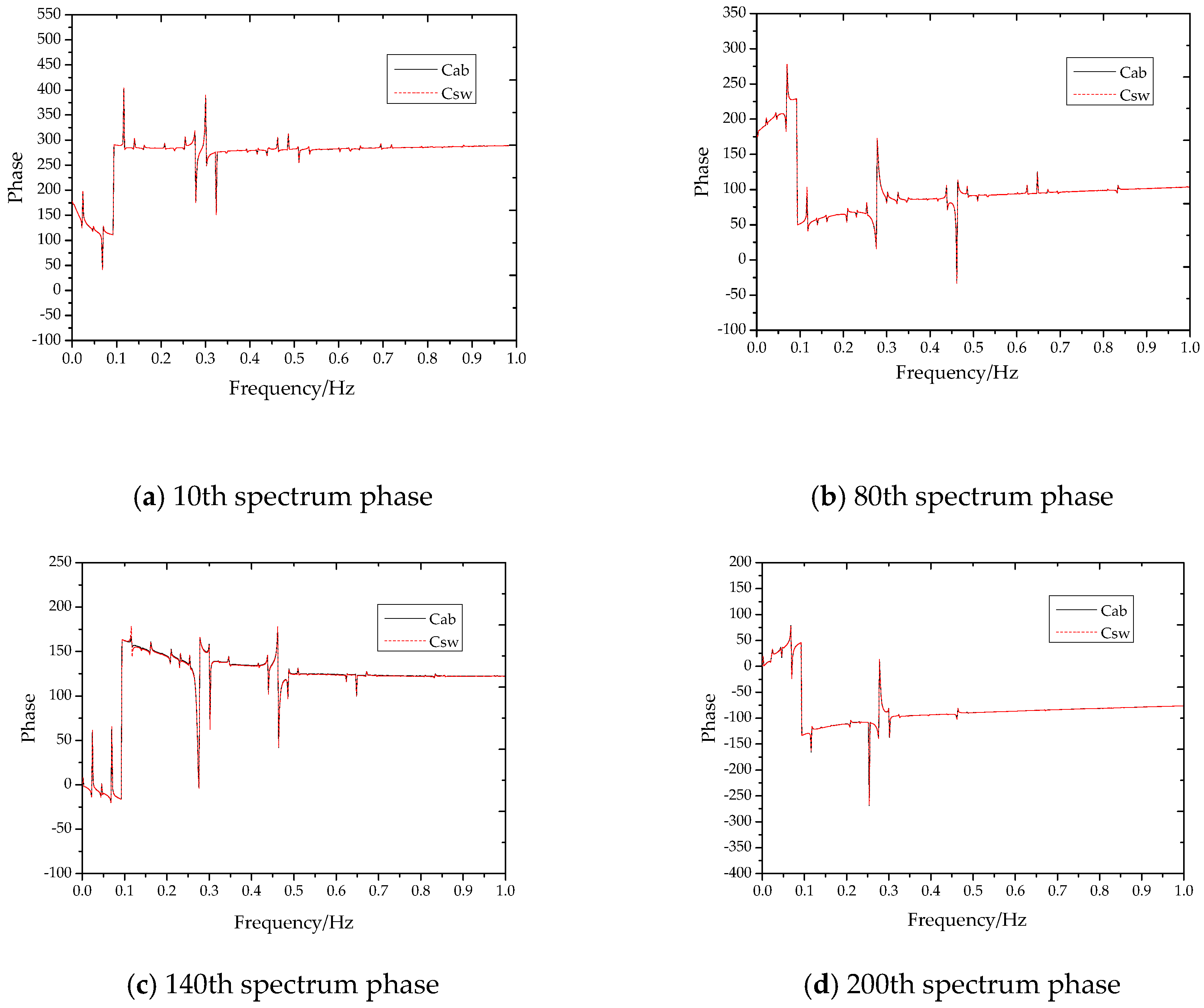
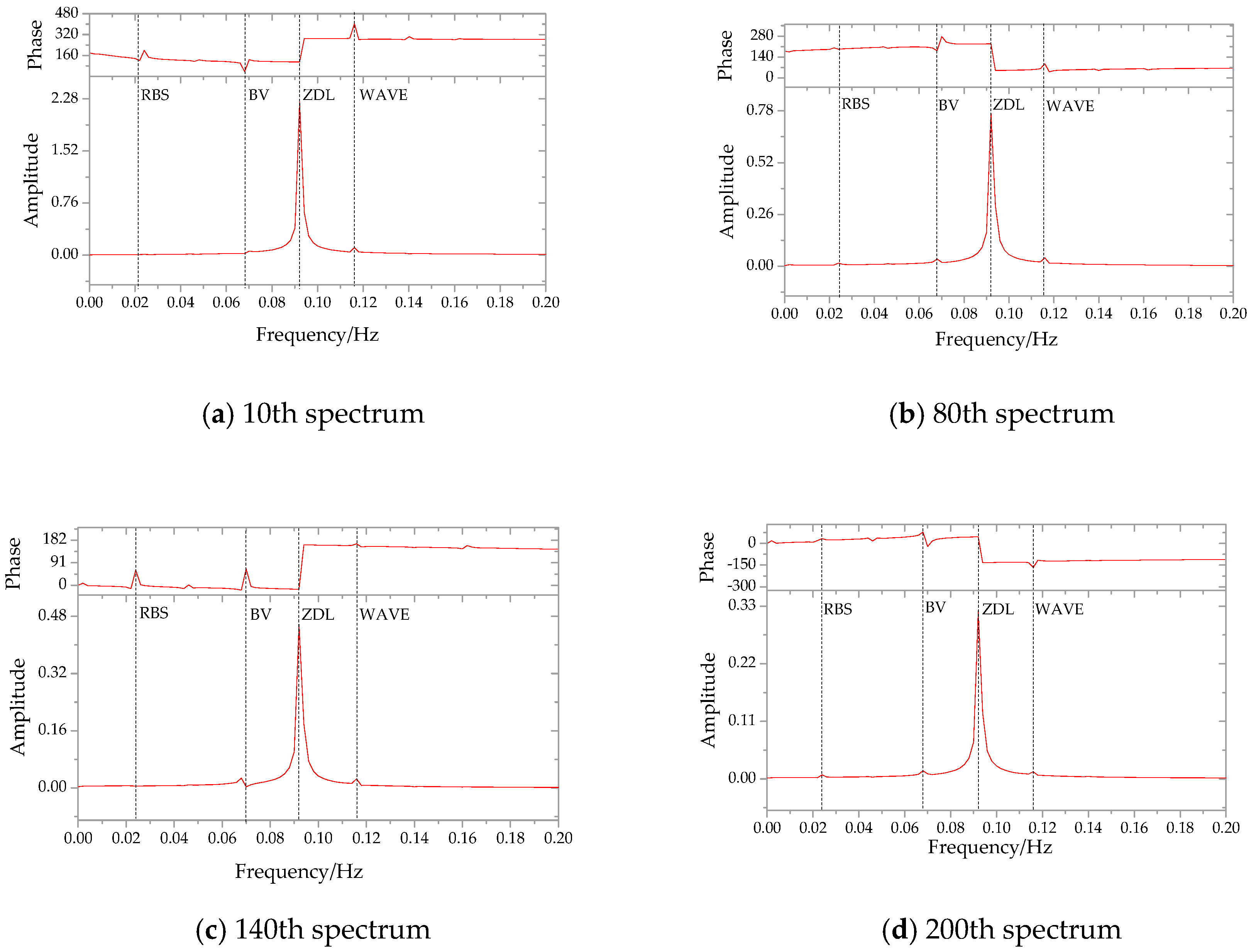
4.4.4. Analysis of the Structural Phase Response

The main frequency and other frequencies of the structure are usually obtained by a frequency amplitude graph. The phase diagram has a relatively obvious relations with the frequency which is a good complement to the amplitude analysis in this paper.

The influence of structural frequency can be obtained by analyzing the phase of the 10th–200th nodes in Figure 18 in working condition 1. Cliffs or rapid changes occur in the structures at frequencies of 0.1 Hz, 0.3 Hz and 0.4 Hz. This means the structures are affected by obvious loads such as waves here. 0.1 Hz is the effect of the wave load. The response frequencies 0.3 Hz and 0.4 Hz are the structure’s natural vibration frequency influenced by the term n². Due to the effect oft the term n², the loads of waves and the suspension point in the z direction and rigid body swing have higher order effects. Specifically speaking, they have second and third order effects at 0.3 Hz and 0.4 Hz.

4.5. The Summary of Response Analysis

In terms of the overall spatial motion, the structure is affected by the mutual loads perpendicular to each other. The response is gradually complicated along with the water depth. The characteristics of oscillations with or without rigid body are studied in this paper. The main frequency and other frequencies are obtained by a frequency amplitude graph. The phase diagram has a relatively obvious resolution to frequency and it is a good complement to the response analysis.

5. Conclusions

Based on the analysis of vibration theory, a SCR model is simulated and analyzed for the rigid body swing’s influence. The characteristics of oscillations caused by water depth and with rigid body swing are researched in this paper. The spectrum amplitude and phase are adopted for analysis of main frequency. The main conclusions of this work are as follows:

(1)

Program for rigid body swingares few and their iteration is relatively complex. For structural design it is relatively appropriate to consider the influence of rigid body swing by multiplying the response of the main load by a coefficient. According to the statistics of multiple conditions described in this paper, the influence coefficient range of displacement is −0.02–0.02 and the influence coefficient range of the main frequency amplitude is −0.007–0.002.

(2)

Waves are perpendicular to the rigid body swing and load of the suspension point in the z direction in this paper. The analysis of the Lissajous curve for qualitative verification and spectral phase for quantitative verification together can provide a relatively good verification for the rigid body swing.

(3)

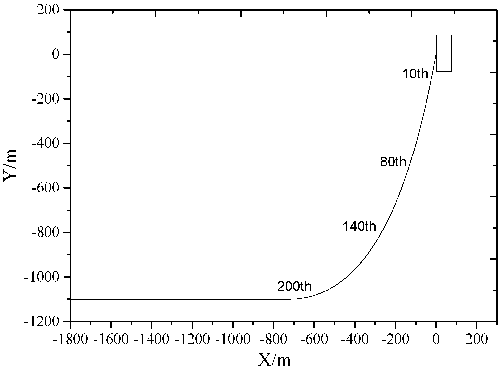
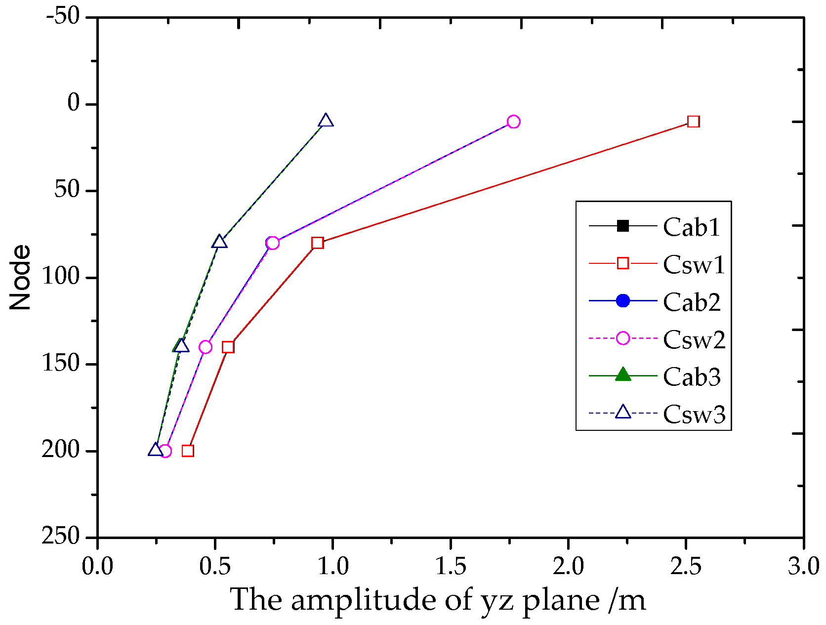
In terms of overall spatial movement, the response is gradually complicated along the depth. The motion response varies from the yz plane at the 10th node to the zx plane at the 200th.There is a rotation around the z axis in this process. There are phase differences between rigid body swing, wave and the load of the suspension point in the z direction. The structural response is related to the conditions and its trend is relatively uncertain. As an influencing term, the effect of rigid body swing with depth displays a positive linear correlation with the diameter vector S.

The response and main frequency have different attenuations at different nodes with depth. The response of the topside 10th–80th region has a sharp decrease, while the response of the 80th-bottom region has a smaller decrease. The response of nodes shows a strong positive correlation with the load of suspension point in the z direction. And it is a forced motion. For the response in top region, it poses a threat to the SCR as a whole for its large amplitude, fast attenuation and strong intensity plane vibration.

(4)

In terms of frequency analysis, the result of the rigid body swing frequency solved by the Rayleigh method and the natural frequency of the bending vibration solved by the simply supported beam method are close to that of the FFT transformation. This can relatively meet the requirements of verification for further research. After a spectrum analysis, the results reveal that the load frequency of the suspension point in the z direction is the main frequency. In addition, the main load frequencies of the structure do not resonate with the frequency of the bending vibration. For phase analysis, the trajectory curve under load changes, and the phase curve will show a cliff or rapid change. On the contrary, this kind of variation can distinguish structural load frequencies well. In terms of deficiencies and prospects of this work, there is no real platform load and nonlinear calculation such as random wave. It is still necessary to continue to research the influence in a more realistic environment.

References

1. Huang, W.P.; Li, H.J. A New type of deepwater riser in offshore oil & gas production:the steel catenary, SCR. Period. Ocean Univ. China 2006, 36, 775–780. [Google Scholar]
2. Zhu, H.J.; Gao, Y. Vortex induced vibration response and energy harvesting of a marine riser attached by a free-to-rotate impeller. Energy 2017, 134, 532–544. [Google Scholar] [CrossRef]
3. Qiu, W.; Lee, D.Y.; Lie, H.; Rousset, J.M.; Mikami, T.; Sphaier, S.; Tao, L.B.; Wang, X.F.; Magarovskii, V. Numerical benchmark studies on drag and lift coefficients of a marine riser at high Reynolds numbers. Appl. Ocean Res. 2017, 69, 245–251. [Google Scholar] [CrossRef]
4. Li, H.J.; Wang, C.; Liu, F.S.; Hu, S.J. Stress wave propagation analysis on vortex-induced vibration of marine risers. China Ocean Eng. 2017, 31, 30–36. [Google Scholar] [CrossRef]
5. Teixeira, D.C.; Morooka, C.K. A time domain procedure to predict vortex-induced vibration response of marine risers. Ocean Eng. 2017, 142, 419–432. [Google Scholar] [CrossRef]
6. Xu, J.; Wang, D.S.; Huang, H.; Duan, M.L.; Gu, J.J.; An, C. A vortex-induced vibration model for the fatigue analysis of a marine drilling riser. Ships Offshore Struct. 2017, 12, S280–S287. [Google Scholar] [CrossRef]
7. Cabrera-Miranda, J.M.; Paik, J.K. On the probabilistic distribution of loads on a marine riser. Ocean Eng. 2017, 134, 105–118. [Google Scholar] [CrossRef] [Green Version]
8. Do, K.D.; Lucey, A.D. Boundary stabilization of extensible and unshearable marine risers with large in-plane deflection. Automatica 2017, 77, 279–292. [Google Scholar] [CrossRef]
9. Zhang, X.D.; Gou, R.Y.; Yang, W.W.; Chang, X.P. Vortex-induced vibration dynamics of a flexible fluid-conveying marine riser subjected to axial harmonic tension. J. Braz. Soc. Mech. Sci. Eng. 2018, 40, 8. [Google Scholar] [CrossRef]
10. Liu, J. Study of Out-Of-Plane Motion of SCRs with Rigid Swing. Ph.D. Thesis, China Ocean University, Qingdao, China, 2013. [Google Scholar]
11. Yao, X.L. On the Dynamic Response and Fatigue of Steel Catenary Riser with Rigid Swinging. Ph.D. Thesis, China Ocean University, Qingdao, China, 2018. [Google Scholar]
12. Komachiy, M.S.; Tabeshpour, M.R. Wake and structure model for simulation of cross-flow/in-line vortex induced vibration of marine risers. J. Vibroeng. 2018, 20, 152–164. [Google Scholar]
13. Domala, V.; Sharma, R. An experimental study on vortex-induced vibration response of marine riser with and without semi subm-ersible. Proc. Inst. Mech. Eng. Part M J. Eng. Marit. Environ. 2018, 232, 176–198. [Google Scholar]
14. Hong, K.S.; Shah, U.H. Vortex-induced vibrations and control of marine risers: A review. Ocean Eng. 2018, 152, 300–315. [Google Scholar] [CrossRef]
15. Alfosail, F.K.; Nayfeh, A.H.; Younis, M.I. A state space approach for the eigenvalue problem of marine risers. Meccanica 2018, 53, 747–757. [Google Scholar] [CrossRef]
16. Yang, W.W.; Ai, Z.J.; Zhang, X.D.; Gou, R.Y.; Chang, X.P. Nonlinear three-dimensional dynamics of a marine viscoelastic riser subjected to uniform flow. Ocean Eng. 2018, 149, 38–52. [Google Scholar] [CrossRef]
17. O’Halloran, S.M.; Harte, A.M.; Shipway, P.H.; Leen, S.B. An experimental study on the key fretting variables for flexible marine risers. Tribol Int. 2018, 117, 141–151. [Google Scholar] [CrossRef]
18. Wang, X.H.; Guan, Z.C.; Xu, Y.Q.; Tian, Y. Signal analysis of acoustic gas influx detection method at the bottom of marine riser in deepwater drilling. J. Process Control. 2018, 66, 23–38. [Google Scholar] [CrossRef]
19. Hu, Y.L.; Cao, J.J.; Yao, B.h.; Zeng, Z.; Lian, L. Dynamic behaviors of a marine riser with variable length during the installation of a subsea production tree. J. Marine Sci. Technol. 2018, 23, 378–388. [Google Scholar] [CrossRef]
20. Yang, J.X. Study on the properties of Lissajous’ Figures. J. Xihua Univ. Nat. Sci. 2008, 27, 98–100, 125. [Google Scholar]
21. Yang, J.X. Study on the synthesized Path of Two Simple Harmonic Vibrations with one Vertical to another. J. Xihua Univ. Nat. Sci. 2008, 2, 5, 76–78, 82. [Google Scholar]
22. Li, J.W.; Tang, Y.G.; Li, Y. Influence of areodynamic imbalance on an offshore wind turbine during pitch controller fault. Ocean Eng. 2017, 35, 37–43. [Google Scholar]
Figure 1. Process of the structural model.
Energies 12 00273 g001
Figure 2. Coordinate system of the beam.
Energies 12 00273 g002
Figure 3. Rigid body swing system.
Energies 12 00273 g003
Figure 4. Petrobras Marlim oil and gas fields.
Energies 12 00273 g004
Figure 5. Lissajous phenomenon of 10th–200th in the zx plane.
Energies 12 00273 g005
Figure 6. Lissajous verification table.
Energies 12 00273 g006
Figure 7. The static location.
Energies 12 00273 g007
Figure 8. 10th–200th three dimensional response of no rigid body swing.
Energies 12 00273 g008
Figure 9. 10th–200th two-dimensional response of a/no rigid body swing in the yz plane.
Energies 12 00273 g009
Figure 10. Amplitude change with water depth.
Energies 12 00273 g010
Figure 11. Amplitude change with conditions.
Energies 12 00273 g011
Figure 12. 10th–200th z-direction time history response in condition 1.
Energies 12 00273 g012
Figure 13. 10th–200th z-direction response changing with conditions.
Energies 12 00273 g013aEnergies 12 00273 g013b
Figure 14. z-Direction response in conditions 1–3 changing with the nodes.
Energies 12 00273 g014
Figure 15. 10th spectrum of condition 1.
Energies 12 00273 g015
Figure 16. 10th–200th spectrum of condition 1.
Energies 12 00273 g016
Figure 17. 10th–200th spectrum amplitude of condition 1.
Energies 12 00273 g017
Figure 18. 10th–200th spectrum phase of condition 1.
Energies 12 00273 g018