Water and Energy Efficiency Improvement of Steel Wire Manufacturing by Circuit Modelling and Optimisation


1
Instituto de Soldadura e Qualidade, 4415-491 Grijó, Portugal
2
Departamento de Engenharia Química, Instituto Superior Técnico, 1049-001 Lisboa, Portugal
3
Departamento de Engenharia Mecânica, Faculdade de Engenharia da Universidade do Porto, 4200-465 Porto, Portugal
4
Dechema Research Institute, 60486 Frankfurt am Main, Germany
*
Author to whom correspondence should be addressed.
Energies 2019, 12(2), 223; https://doi.org/10.3390/en12020223
Submission received: 29 November 2018
/
Revised: 2 January 2019
/
Accepted: 3 January 2019
/
Published: 11 January 2019
(This article belongs to the Special Issue Energy Efficiency in Electric Devices, Machines and Drives)
Abstract
:Industrial water circuits (IWC) are frequently neglected as they are auxiliary circuits of industrial processes, leading to a missing awareness of their energy- and water-saving potential. Industrial sectors such as steel, chemicals, paper and food processing are notable in their water-related energy requirements. Improvement of energy efficiency in industrial processes saves resources and reduces manufacturing costs. The paper presents a cooling IWC of a steel wire processing plant in which steel billets are transformed into wire. The circuit was built in object-oriented language in OpenModelica and validated with real plant data. Several improvement measures have been identified and an optimisation methodology has been proposed. A techno-economic analysis has been carried out to estimate the energy savings and payback time for the proposed improvement measures. The suggested measures allow energy savings up to 29% in less than 3 years’ payback time and water consumption savings of approximately 7.5%.
1. Introduction
Industrial Water Circuits (IWCs) encompass all the water streams of a factory unit, including the most common uses of water industrially such as water cooling and water treatment. Such processes are responsible for significant consumption of water as well as energy. The industrial sector is responsible for 20% of the total water consumption in the world [1], while in terms of energy it represents 30% of the global final end-use of energy [2]. The European industry in particular is responsible for 40% of the total water abstractions [3] and 25% of the final end-use of energy in the European Union is attributed to this sector [4]. Electric motors, in turn, represent 65% of the total electric energy consumption in European industry [5] and pumping systems in particular account for 21% of the aforementioned share of electricity consumption [6]. These figures show that it is crucial to improve the energy efficiency of IWCs.
The 2012 Energy Efficiency Directive [7] and implementing directive for the Ecodesign requirements for water pumps [8] focus on reducing energy consumption and consequently, water consumption. These directives emerged in the scope of the climate change and energy targets of the Europe 2020 Strategy [9]. Hence, increasing attention have been given to alternative strategies for the reduction of energy and water consumptions.
The European project WaterWatt [10] aims to develop new tools and guidelines to reduce energy consumption in IWCs. IWCs are generally treated as secondary streams in the production process of a plant and therefore neglected. Furthermore, the associated energy consumption is frequently despised, as the circuits only represent a minor part of the total electricity consumption. In this alignment, the present paper presents an object-oriented model, developed in the open source OpenModelica Software in order to analyse and improve the energy consumption of an IWC case study part of the WaterWatt project [11].
The optimisation problems approached in this work are based on the application of improvement measures to reduce electric energy consumption and water consumption in IWC. The measures for energy efficiency improvement in IWC, and similar systems such water networks and water distribution systems, have been proposed by several authors. Cabrera et al. [11] proposed two sets of strategies for energy efficiency improvement, an operational-type set and structural-type set. In operational group, it was proposed: the operation of the pumping systems at the best efficient point (BEP), the improvement of the system regulation to avoid surplus energy, the minimization of leaks and the minimization of friction losses. For the structural group, it were proposed: the use of more efficient pumps, the decoupling of energy sectors and the improvement of designs and layouts.
As part of the WaterWatt project and this work specifically, the optimization based on energy efficiency improvement of the IWC will be performed taking into account the knowledge about the proposed measures for this type of systems and the knowledge about the achievement of energy savings by the adjustment of the operation of electric motors. The application of variable speed drives (VSD) in electric motors is proposed to attain considerable reductions in both water and energy consumptions, which in the case of the pumping systems it has been revealing as an excellent alternative to currently applied improvement measures.
In this paper, different improvement measures are proposed, and energy savings and payback associated to these are estimated. The case study corresponds to water cooling circuit of a steel wire processing plant in Germany in which steel billets are transformed into wire. In general, iron and steel industry present an electrical energy consumption of 2327 ktoe/year, which represents about 12% of the total energy consumption of the industrial sector namely in Germany [12]. Moreover, the production of basic metals in the manufacturing industry in Germany has a total water consumption of about 581 dam3, in which 85% corresponds to water cooling [13].
2. Model Assembling
2.1. Circuit Description
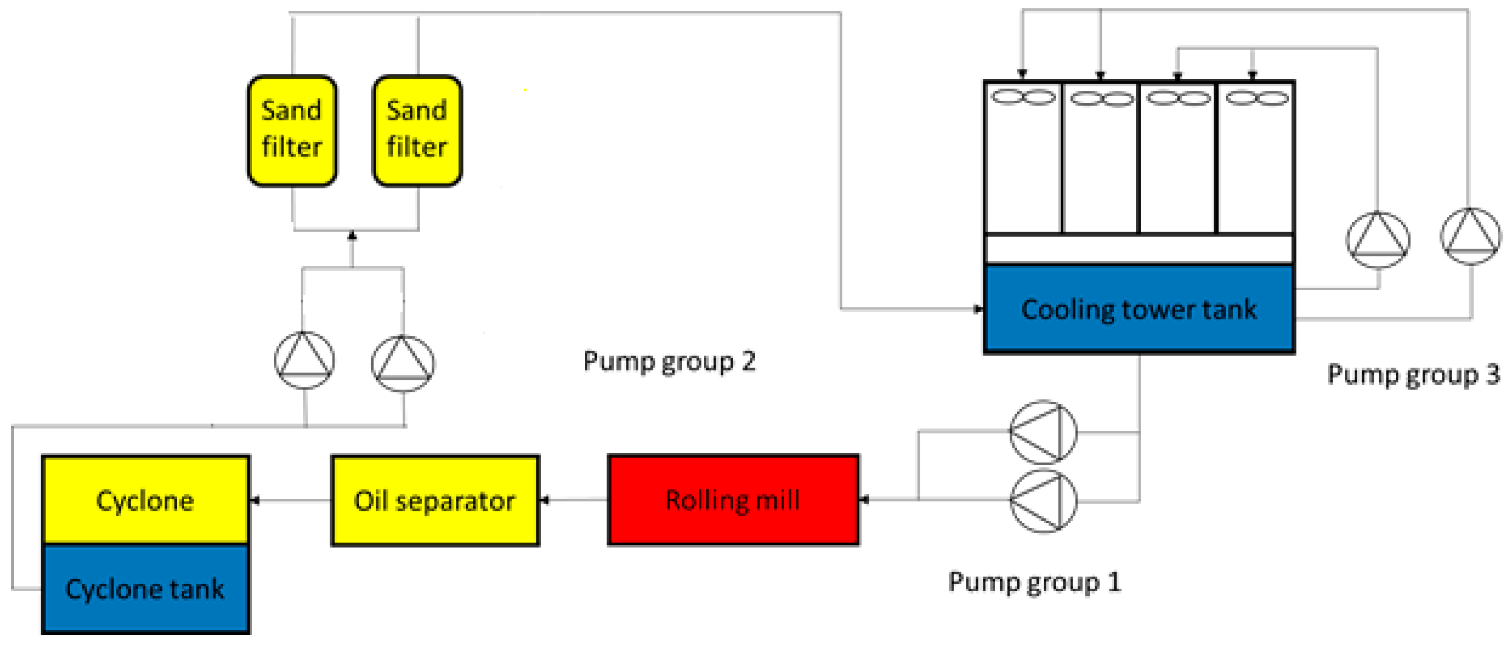
The cooling circuit under analysis includes a hot roiling mil, four cooling towers, three pump groups, four sand filters, one oil separator and a cyclone separator (Figure 1). The pump group 1 is constituted by two pumps that transport cooled water from a tank (Cold Water Tank) to the rolling mill. Then, the water stream flows down the channel to an oil separator and cyclone (Cyclone Tank) for the pre-treatment of water. The pre-treated water is distributed to two sand filters by the action of pump group 2, constituted by two pumps in operation. From the sand filters, the water stream flows back to the cooling tower tank. The designated pump group 3 is part of a secondary circuit, constituted by two pumps. Pump group 3 corresponds to the same type as pump groups 1 and 2 to reduce maintenance and logistic effort. This separate water stream is transported from the cooling tower tank to the four cooling towers and the outlet water streams from the cooling tower are then, transported back to the tank. This secondary circuit is part of a recent modernisation drive in the factory. Such modernization aims to improve energy efficiency. It was installed to allow the operation of the cooling towers only when required (i.e., when the temperature at the cold water tank increases above the operational target-value by 0.5 °C) and as soon as temperature drops the circuit stops. For instance, this may constitute a constraint for the process optimization based on energy efficiency improvement, in which the temperature of the cold water tank must not be exceeded by 0.5 °C relatively to its target-value. Otherwise, this operational requirement is considered to be surpassed. The separation of the cooling towers from the main circuit also allows a closer control on the cooling process as the water demand in the circuit is variable. This is because the billets are produced in batches and due to the existence of variabilities in the material and the rolling mill operational conditions, such as rolling speed and cooling speed.
The inlet water stream in the rolling mill is used for the main purpose of direct and indirect cooling. Nonetheless, it used in the remaining processes of hot forming, such as descaling and scale transport. For that reason, a water treatment section is installed after the hot forming process. This section is constituted by the filtration units, constituted each one, by two sand filters. Moreover, it is preceded by an oil separator and a cyclone, constituting a pre-treatment section.
Table 1 summarizes the specifications for the design and assembling of the model circuit (described Section 2.2).
The heat input at the hot rolling mill (qinput,RM) is determined by:
where Q1 and Q2 corresponds to the water flowrate of the main and secondary circuit respectively (Table 2). The density of the water (ρw) corresponds to 999 kg/m3 and the specific heat (cpw) to 4.186 kJ/kg°C. The Tinlet_RM is determined by:
whereas:
qRMinput = Q1 × ρw × cpw × (TRMinlet − TRMoutlet)
Q1 × ρW × CP,w × (Tin,1 − Tout,1) = Q2 × ρW × CP,w × (Tin,2 − Tout,2)
Tout,1 = TRMinlet
These two additional inputs of the circuit are listed in Table 2.
The measurements at the plant included the water temperature, water flowrate and pressure drop across pumps and sand filters (Table 3). In order to measure the flowrate, ultrasonic signals have been used, employing the transit time difference principle. The ultrasonic signals are emitted by a transducer installed on the pipe and received by a second transducer. The transit time difference is measured and allows the flowmeter to determine the average flow velocity along the propagation path of the ultrasonic signals. A flow profile correction is then performed to obtain the area averaged flow velocity, which is proportional to the volumetric flow rate. Two integrated microprocessors control the entire measuring process, removing disturbance signals, and checking each received ultrasonic wave for its validity which reduces noise. Moreover, the temperature of the water circulating within the pipes was measured by coupling two resistance thermometer (RTD) temperature probe (applicable to the supply and return pipes simultaneously) whose outputs are integrated with the flow measurements at the meter. The pressure drops across pumps and filters have been measured by the coupling of manometers before and after each component. Also, the power of pumps have been recorded during representative period of time. This has been performed by a power analyser connected to a data logger, taking three phase power measurements by coupling clamp meters into the phases. Table 1 summarizes the specifications for the design and assembling of the model circuit (described Section 2.2).
2.2. Design and Assembling of IWC Model
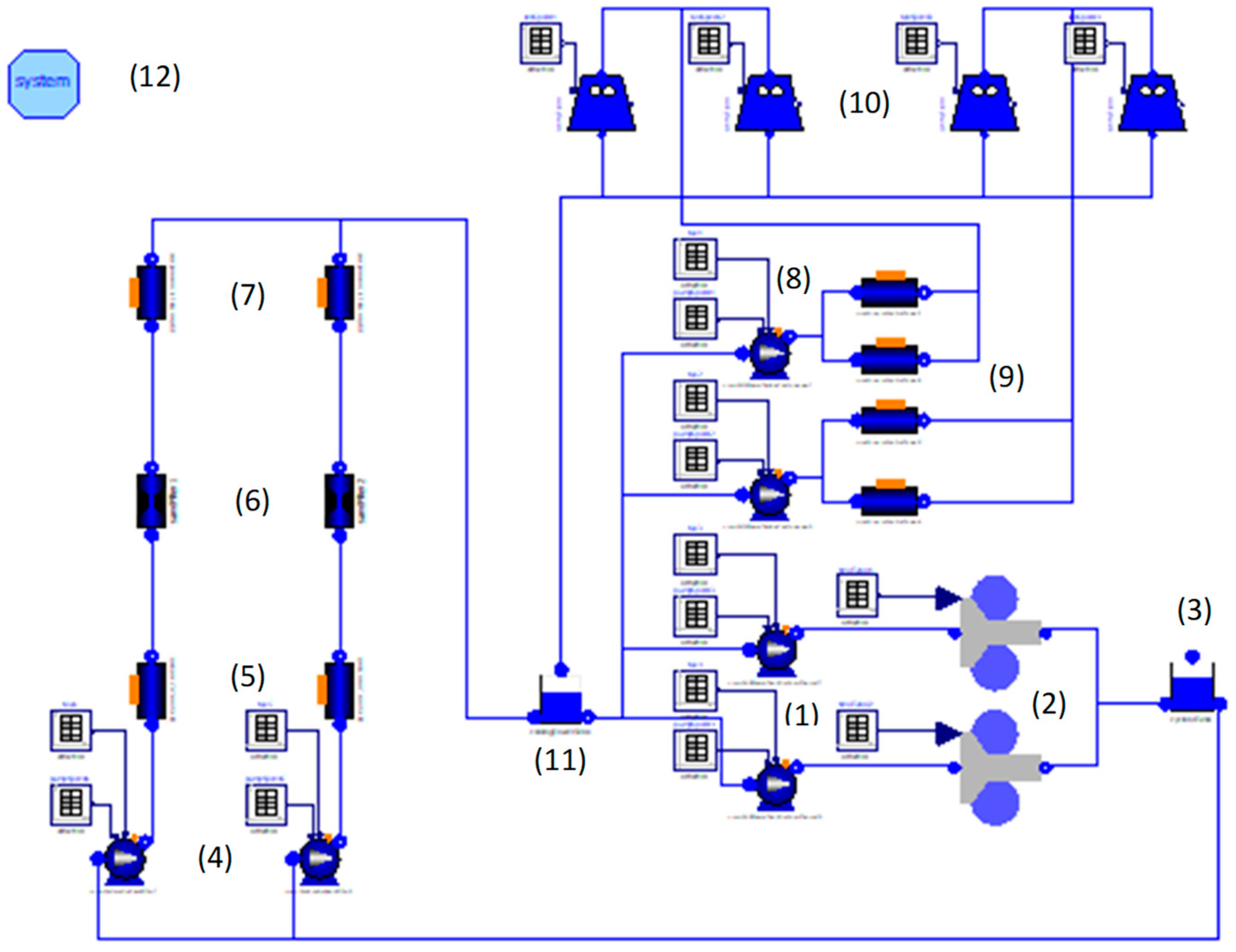
The IWC was built in the object-oriented language in OpenModelica, used for the modelling of such physical systems and supports most of the equipment (Figure 2).
Currently, a number of free and commercial component libraries in different domains are available, including electrical, mechanical, thermo-fluid and physical-chemical. The current case study was built using the ThermoPower library [14] that has been developed with the goal of providing a solid foundation for dynamic thermal and power modelling. It includes a list of components, such as pumps, tanks, cooling towers, pipes and filters, that can be “drag and drop” for the modelling assembling. Each component corresponds to singular model to be setup accordingly with the required parameters and therefore, replicability is assured.
The selected components and respective models correspond to the main components of the circuit namely: tank model, pump model, pipe model, filter model, cooling tower model and rolling mill as further described. Each model was accordingly setup using the measured data collected in the case study circuit and presented in the beginning of this section.
2.2.1. Tank Model
The model represents a free-surface water tank corresponding to the vertical axis in the region where the fluid level is supposed to lie within. The tank geometry is described the input parameters: V0 (volume of the fluid when the level is at reference zero height), A (cross section of the free surface) and y0 (height of “zero-level”). The model also requires the input parameters ymin and ymax, which should be appropriate to avoid underflow or overflow of the tank. The pressure at the inlet and outlet ports accounts for the ambient pressure and the static head due to the level, while the pressure at the inlet port corresponds to the ambient pressure.
Concerning the mass and energy balances the model assumes there is no heat transfer except through the inlet and outlet flows. It is to note that, due to the inexistence of the performance of heat transfer directly in the modelling of the cold water tank in the present IWC, the sand filters outlet water streams are cooled through the contact with the water stream from the secondary circuit at a lower temperature.
2.2.2. Pump Model
The model represents a centrifugal pump, or rather a group of centrifugal pumps in parallel. The input parameters are related with the pump curves therefore defined in the model for each single pump or pump group. The component characteristics are given for nominal conditions of flowrate and rotational speed. These characteristics may be then adapted according to similarity equations, namely the affinity laws for the pumps to different flow conditions (Equation (7)).
There are two input functions: flowCharacteristic that corresponds to the relationship of the volumetric flowrate and the head, while the efficiencyCharacteristic, corresponds to the relationship between the volumetric flowrate and the hydraulic efficiency. One of the output parameter is the electric power of the pump (Pump). This also accounts for the mechanical efficiency of the pump motor (motorEfficiency) also set as input.
In addition to the inlet and outlet ports of the water stream, the pump models also include inlet ports for the motor speed (in_n), the electricity tariff (tax) and the number of pumps in parallel (in_NP).
2.2.3. Pipe Model
The model represents the piping system of the circuit, either as a single tube or by N parallel tubes, representing the water flow streams of the factory unit. It is built with certain assumptions, such as: one-phase fluid state, uniform velocity across the section, constant turbulent friction, longitudinal heat diffusion is neglected and uniform pressure distribution in the energy balance equation.
The finite volume method is used to discretize the mass, momentum and energy balance equation, taking as the state variables one pressure, one flowrate and N-1 specific enthalpies. The dynamic momentum is not accounted by default.
The input parameters for the pipe model are: the pressure losses on the pipes due to the friction phenomena (dpnom) and the static head (h) as well as the mass flowrate (wnom). In addition to the inlet and outlet ports of the water stream, the pipe model also contains a wall-type inlet (wall), which can be specified for a certain heat input. Taking into account that the circuit pipes are all installed at the same level, this is, it does not exist pressure losses due to elevation, the total pressure drop of the sections of the piping system are determined considering the head losses due the friction of the pipes, according to:
The friction factor (f) was determined using the Moody pipe friction chart, according to a transitional flow regime (Re = 24,300). Moreover, for the total head losses the minor losses are also considered. The minor losses consist of the local pressure drop (Equation (5)) due to sudden or gradual expansion or contraction, the presence of bends, elbows, tees and valves (open or partially closed).
The KL is determined according to tabulated values for each type of local pressure drop [15].
2.2.4. Filter Model
The model is set to induce and determine the pressure loss in the circuit. The pressure drop across the inlet and outlet connectors of the components is proportional to the square velocity of the fluid, defined according to a turbulent friction model. The input parameter corresponds to the pressure drop across de filter (dpnom).
2.2.5. Cooling Tower Model
The model represents an open cooling tower with fans and it is filled with metallic packaging. The humid ambient air is used to cool the incoming water stream. The fluid is modelled using the IF-97 water-steam model as an ideal mixture of dry air and steam.
The hold-up of water in the packaging is modelled assuming a linear relationship between the hold-up in each volume and the corresponding outgoing flow. The finite volume method is used to discretize the corresponding 1-D counter-current equations. The Merkel’s equation [16] is used for the mass and heat transfer phenomena from the hot water to the humid air (Equation (6)):
Note that k designates the overall heat and mass transfer coefficient and S the surface of packing. The required input parameters correspond to: the overall mass and heat transfer (k_wa_tot), nominal water mass flowrate (wlnom), nominal air volume flow rate (qanom), normal air density (rhoanom), surface of packing (S), nominal fan rotational speed (rpm_nom) and the nominal power consumption (Wnom). The fan behaviour is modelled by kinematic similarity: the air flow is proportional to the fan speed (rpm_nom) and the electric power consumption (Wnom) is proportional to the cube of the speed, according to the affinity laws for the fans (Equations (7) and (8)).
The cooling tower model also contain an inlet port for the fan speed (fanRpm). In which, similarly to the pump motor rotational speed, the fan speed can be changed relatively to the nominal value (in_n). The outcome parameters include the inlet (TCTinlet) and outlet (TCToutlet) ports of the water stream, there is also an outlet port for the electric power consumption of the fan (powerConsumption).
2.2.6. Rolling Mill
The rolling mill connects two models from the ThermoPower library, namely the heat source model and the pipe model already described above. Regarding the heat source model it corresponds to an ideal tubular heat flow source, with uniform heat flux. The actual heating power (P) is provided as input by the power signal connector (in_p). The finite volume method is used for discretisation. The output parameter corresponds to the water outlet temperature (TRMoutlet).
While the comprehension of the thermal phenomena intrinsic in the analysis of this type of circuits have been performed for the design and calibration assuming the more accurate values possible, it is to note that the cooling system of a rolling mill component has been simplified. This represents a thermal power input in the circuit, allowing the increase of temperature proportional to that heat input and water flow rate. Therefore, it still lacks a more complex understanding of the occurrence of phenomena at a more dynamic basis.
2.2.7. System and Time Tables
The System component must be added in any circuit in order to define the system condition, namely water temperature and ambient pressure. In this study, the temperature was considered approximately 15 °C according to the average water temperature provided by the utility company in Germany. The Time Table component allows the user to specify a certain input value over time for a specific component. In the current case study, they are connected to the pump motor and to the fan of the cooling tower to specify the rotational speed of these equipment(rpm). Furthermore, it can also be connected to the rolling mill to specify the thermal input change with time. Additionally, a time table can be connected to specify the electricity tariff price with time.
3. Model Validation
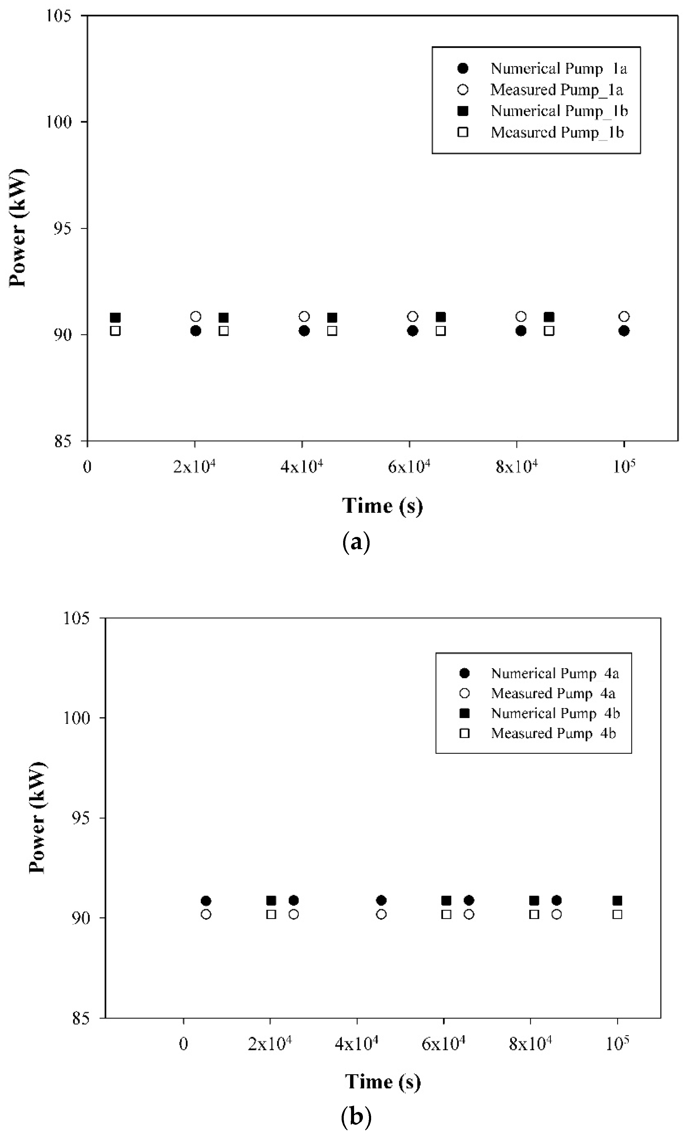
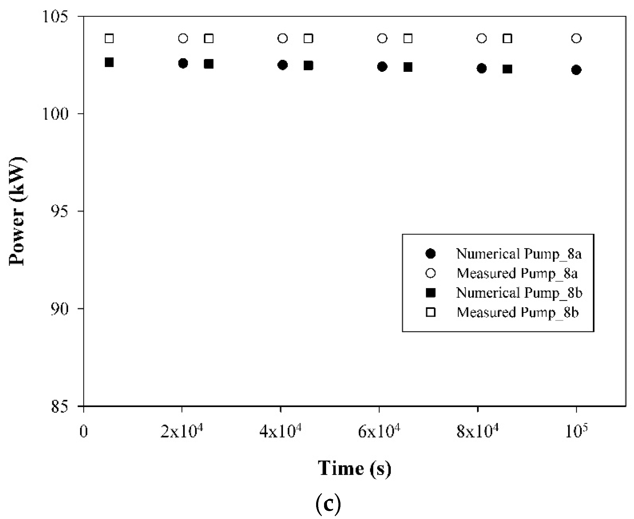
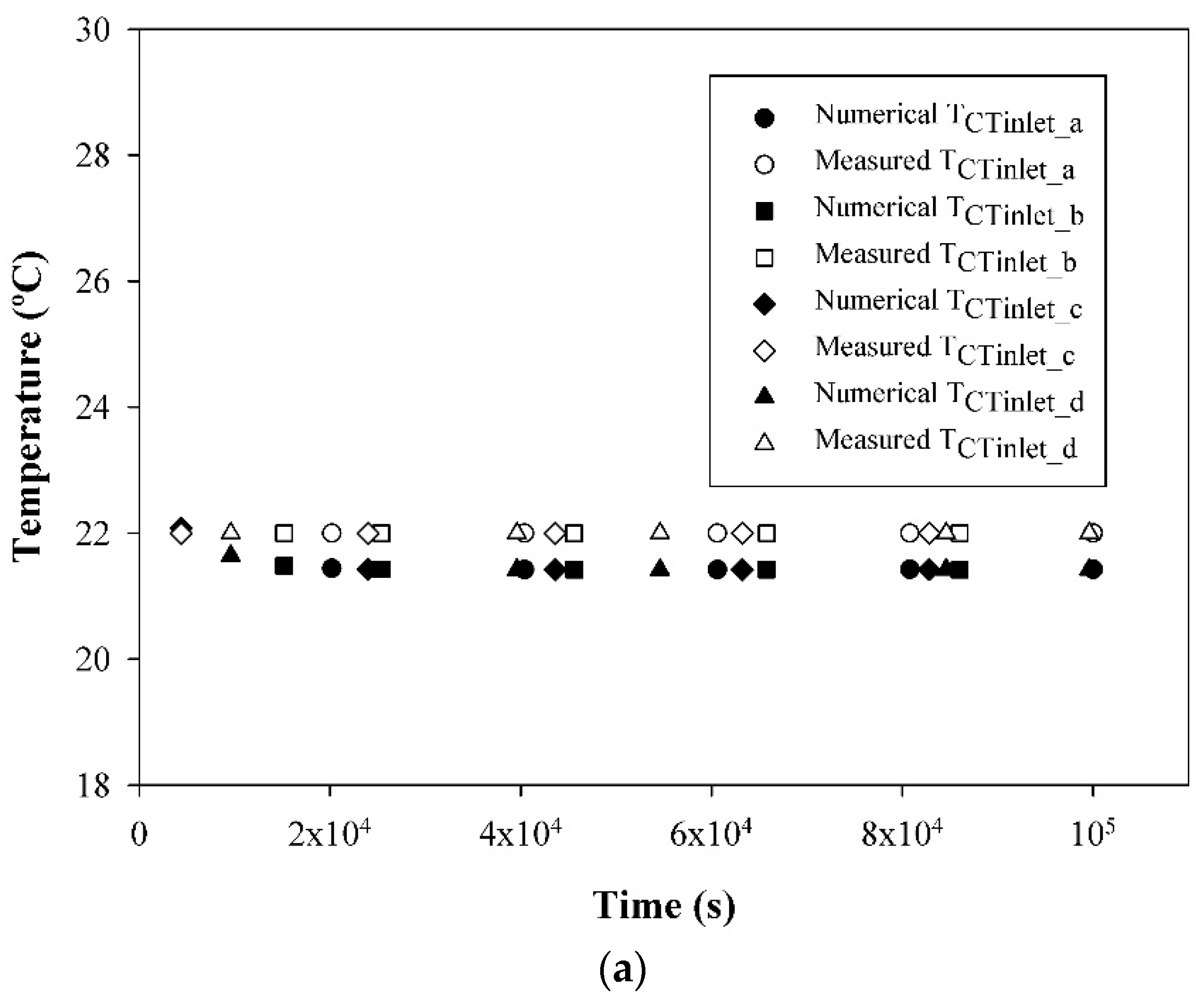
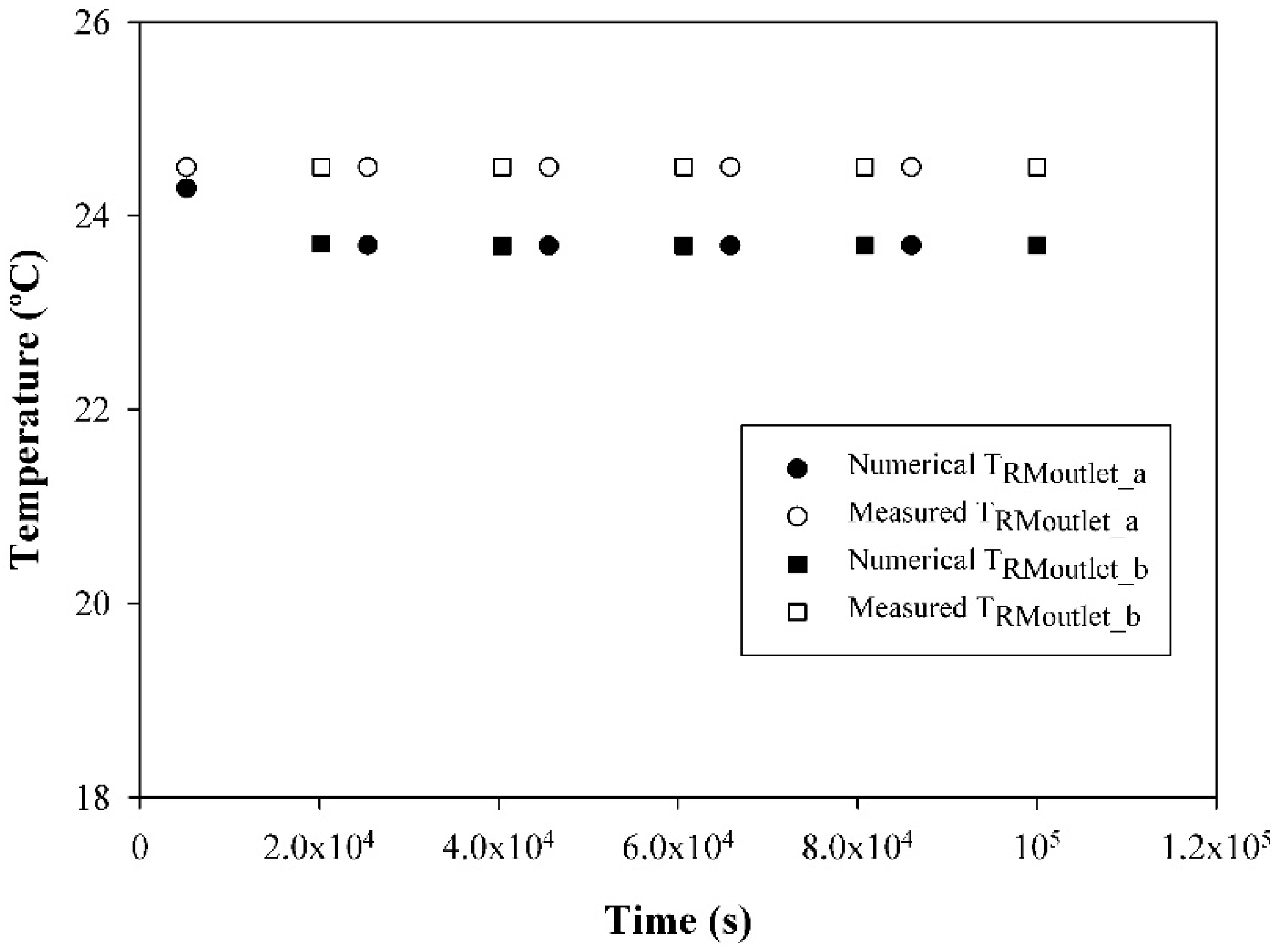
The model results have been validated with real casa data from the case study. For the energy and water consumption the following parameters have been identified for validation: pumps power (Pump1, Pump4, Pump8), the inlet and outlet water temperature at the cooling towers (TCTinlet and TCToutlet) and the water outlet temperature of the rolling mills (TRMoutlet). The outputs of the numerical results for these parameters are presented from Figure 3, Figure 4 and Figure 5.
Furthermore, it is also relevant to analyse the values obtained for the temperatures in different points of the circuit, namely the inlet and outlet water stream temperature at the cooling tower (Figure 4) and outlet water temperature at the rolling mill (Figure 5).
The deviation that has been observed for each pump group to comparison to the nominal value was listed in Table 3 above. The measured electric power used for the operation of the pumps was analysed and validated against plant data and summarized in Table 1. It is observed that the values obtained in the simulation are overall consistent with plant data. Moreover, the value outlet water stream temperature of the hot rolling mill and at the inlet of the cooling towers have minor deviations compared to the real values. The slightly major deviation is related with the outlet temperature at the cooling towers (Table 4). This may be related with the fact that the water circuit in the cooling towers corresponds to a separated circuit from the main circuit. Overall, the thermal phenomena are consistent with plant data and the required cooling load is given by the model.
4. Sensitivity Analysis
A sensitivity analysis of the model was performed. It corresponds to a crucial analysis for the solving of the optimisation problems. The methodology to perform this analysis is distinct from the ones elaborated in dynamic modelling and simulation. As there is a high number of required inputs to be given to the model in order to run, a pre-selection of variables to analysis is required. The selected variables for the analysis correspond to the speeds of pump motor and the cooling tower fan which have a direct influence on power consumption and operational requirements of the IWC. Different scenarios have been defined for these variables (Table 5 and Table 6) to understand their influence on the power consumption (Figure 6). The scenarios have been assembled following a methodology similar to the Monte Carlo method. For this study, is based on random sampling, in which the results for power consumption are obtained for random rotational speeds values. Thus, different values for power consumption are obtained for different scenarios. To note that the best scenarios have been selected based on the lower power consumption of all the pump groups and also without surpassing the operational requirements.
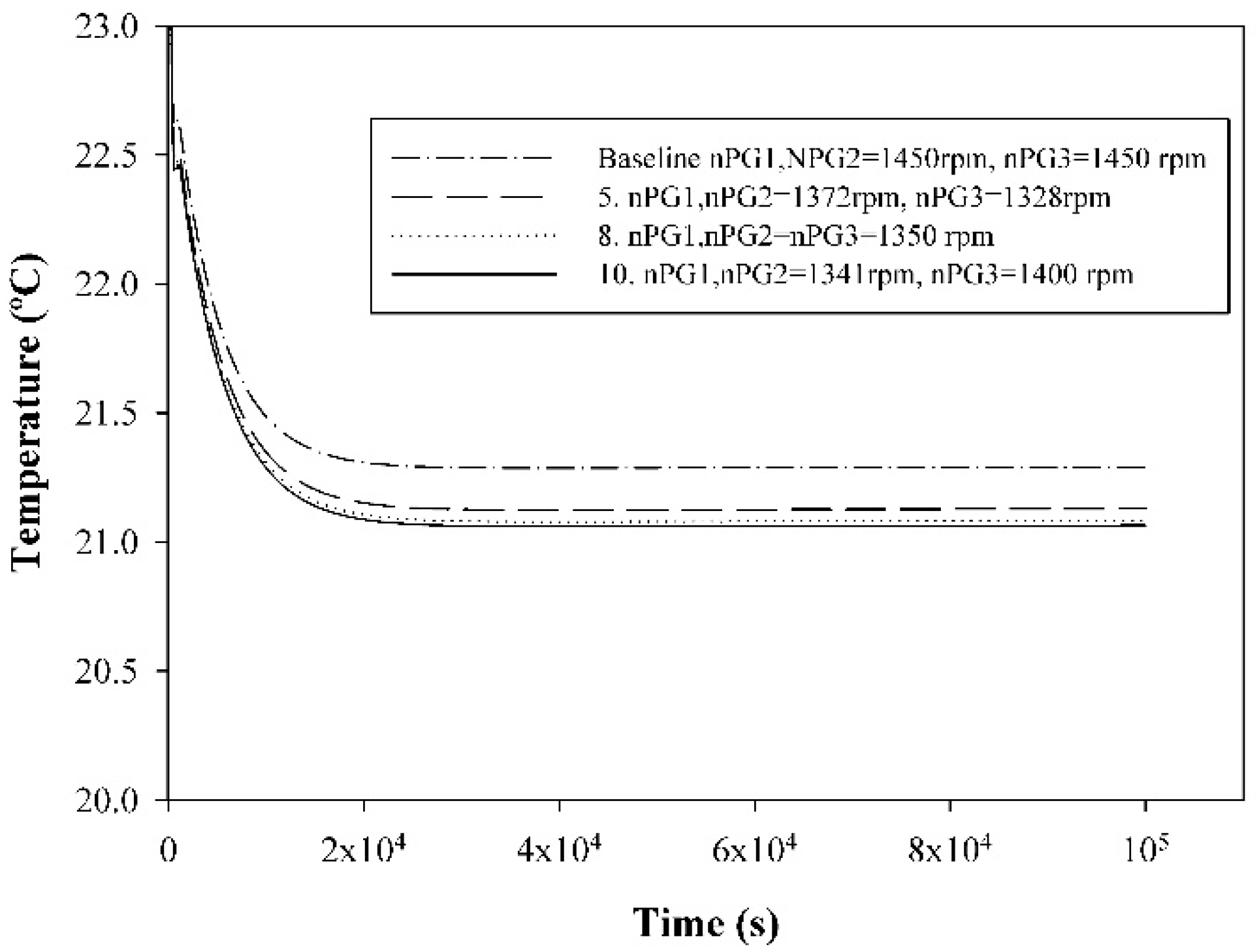
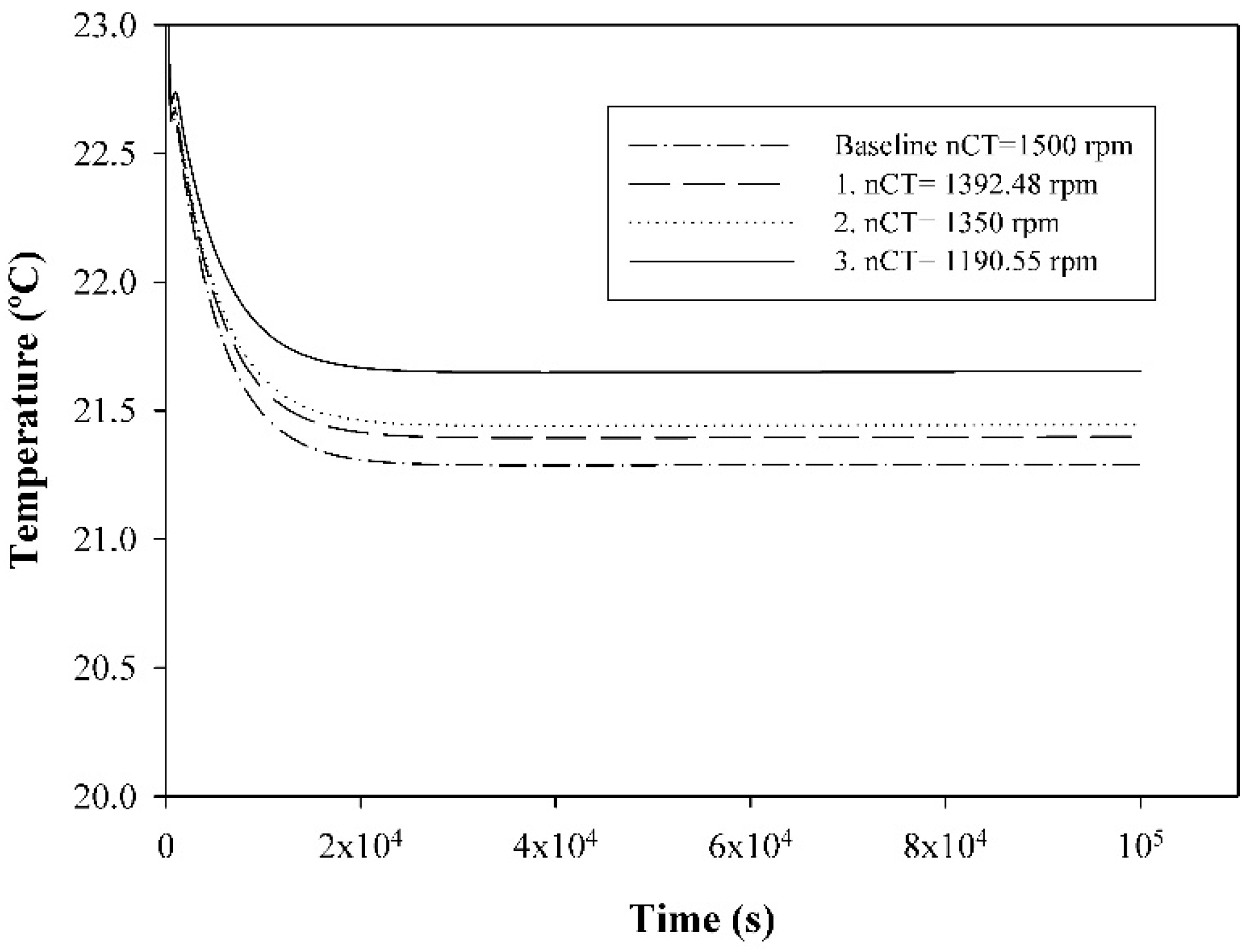
Moreover, it is also necessary to evaluate the influence of those input parameters on simulations results related to temperature and hydraulic parameters. In this study, the influence of the change of the motors speed of pumps and fans (cooling tower) on the water temperature at the cold water tank will be analysed (Figure 7 and Figure 8).
For the sensitivity analysis related with the change of the pump motor rotational speeds, the power consumptions of both pump groups 1 and 2 were analysed simultaneously, since both are part of the main circuit, and having the same technical characteristics. Figure 6 presents the results ten scenarios for the power consumption of pump groups 1, 2 and 3.
From the ten created scenarios, it is necessary to select the ones associated to higher reduction in power consumption of both pump group 1 and 2 and pump group 3. This analysis focuses on the favorable scenarios on the viewpoint of energy efficiency and the possibility of its application. Therefore, observing Figure 6, the three scenarios correspond to 5, 8 and 10 and to be selected to proceed with the sensitivity analysis (Figure 7). The remaining scenarios were neglected, as they do not present significant reduction in power consumption.
The scenarios for the cooling towers (Table 6) were created considering the share of reduction in power consumption by the decrease of the rotational speed of the cooling tower fans, following the affinity laws of the fans (Equation (8)). Thus, three scenarios designated 1, 2 and 3 were created bearing in mind shares of reduction in power consumption of, respectively, 20%, 27% and 50%.
The most efficient scenarios for each case: promoting the major energy reductions in power consumption respecting the operational requirements in temperature, will be analysed furtherly.
5. Identification of Improvement Measures
The efficiency of water circuits can be reached by the dynamic adjustment of the circuit operation to the production process, through the reduction of pressure demand and pressure losses in the circuit and by improvement of energy efficiency of pumps and cooling tower. Such improvements include matching the scale of the motor service to the work demand (i.e., speed control devices such as adjustable speed drives); reducing demand for energy services (e.g., substituting a blower for compressed air or turning off steam supplied to inactive equipment) and the replacement to high efficiency motors. The improvement measures should account for the technical specifications of the process: avoiding interruptions, improvement of production reliability (maintaining required flow, pressure and temperature) and improved maintenance practices. The measures do also account for economic and environmental aspects namely cost reduction, energy savings and reduction of CO2 impact which are the primary aspect that industrials consider regarding energy efficiency.
The present model allows a prior analysis of efficiency measures to be implemented in the IWC avoiding extra costs with technical work. To note that the structural related input variables such as: length and diameter of the pipes, heat inputs in the case of non-looped circuits, despite being highly influential and part of the formulation of certain optimisation problems, they are set as design variables, meaning constant parameters of the assembling of the circuits. Therefore, the analysis of such measures, as related to energy efficiency measures at the design stage and therefore not in the scope of this work.
Furthermore, aim of this work does not focuses on the analysis of process control strategies. Noteworthy such strategies are intrinsic in the operation of all the processes in industry, including the water circuits. Thus, a more accurate analysis of these models would require the comprehension of the models related to types of valves, flowmeters, electric meters and temperature sensors. Such extensions, would possibly assist the operational improvement measures, as well as the application of control related measures. Hence, this paper analyses the application of five improvement measures to the case study circuit in order to reduce the energy and water consumption as well as guaranteeing the required operation conditions.
5.1. Variable Speed Drives (VSD) in Pumps
The coupling of VSD’s allow energy savings of 20% to 25% [17]. The installation of VSD in pump motors allows the automatic flow adjustment to the needs of the process. The change of the pump speed adjusts the pump rotation frequency to the optimal efficiency point. The performance of this measure relies on the affinity laws for the pumps. The automatic flow adjustment is described by Equation (7) [18]:
For the cooling circuit under analysis, the operation of the pump motors was initially set at rotational speed of 1450 rpm for the nominal flowrate. Applying the Equation (7) for the real running flowrate, the optimised rotational speed corresponds to 1350 rpm. New simulations have been performed for the optimal point speed and savings have been estimated and presented in Table 7.
5.2. Refurbishment of Pumps
The refurbishment of pumps corresponds to the mechanical cleaning and overall of a pump to restore its initial functioning, namely its energy efficiency. Pumps without maintenance over the years generate a lower flow. The improvement measure for the pumping system of the case study circuit considered the refurbishment of all pumps. For the calculations, the authors have assumed an improvement of 10% in the hydraulic efficiency of the pump, set in IMechE [19].
5.3. Change of Filters
In water treatment process, sand filters present considerable impact on energy efficiency due to lower pressure drop induced into the water. The improvement measures for the treatment section was to. In replace the two sand filters with a pressure drop of 1.3 bar to new ones with a pressure drop of 0.5 bar. The results are presented in Table 7.
5.4. Change of Electric Motors of the Pumps
The change of electric motors in pumping systems, specifically to electric motors categorized as IE3 Premium Efficiency allow high energy savings. A higher efficiency motor is more expensive than a conventional motor however its lifespan is much longer as it operates at a lower temperature and hence heat losses are lower [20]. In the current circuit, the pump motors with an initial mechanical efficiency of 90% were exchanged to IE3 electric motors with a mechanical efficiency of 95.4%. The savings are presented in Table 7.
5.5. VSD in the Cooling Tower Fans
The installation of VSDs in the cooling tower fans allow a dynamic adjustment of the airflow respecting the required temperature values in the circuit. The power consumption associated to the operation of the fan is directly linked to the fan speed, therefore high energy savings can be achieved with adjustments decreasing the fan speed [21]. The performance of this measure relies on the affinity laws for the fans. The automatic air flow adjustment is described by Equation (7) [22]. Moreover, the change on the power of the fans is described by Equation (8) [18]:
In the circuit under analysis the operation of the four cooling tower fans operates at an initial rotational speed of 1450 rpm. This has been changed to an optimal speed of 1350 rpm. The results are presented in the Table 7.
6. Definition of Optimization Methodology
An optimisation methodology must be developed with the aim to improve energy efficiency in this IWC. This methodology is primarily based on the assembling of several settings for each case, in which a certain input parameter is modified with the aim to achieve lower energy consumption. These are primarily related with the operational conditions of the pumps and cooling towers. The definition of this methodology is necessary for the techno-economic evaluation of the analysed improvement measures. Based on the scenarios assembled in the sensitivity analysis, the objective functions are attained by the changes on the decision variables, although that change must respect the operational requirement of the circuit which are translated by the constraints.
The main objective of the presented optimisation problems is the reduction on electric energy consumption. Although thermal energy consumption is also a relevant concern, and heat is a direct input in certain components of these models, the thermal phenomena are mostly treated as imposed variables of the model, namely as input parameters. Hence, the optimisation methodology includes the definition of objective functions, decision variables and constraints.
The secondary circuit is only switched on when the temperature of the water inside the cold water tank (TCWT) reaches more than 0.5 °C relatively to the target value (22.1 °C). From this, the constraint is defined as a requirement of not exceeding 0.5 °C of the temperature at the cold water tank. This allows to maintain the cooled water temperature close to the required in the cooling process.
The objective functions correspond to the reduction of energy consumption. The decision variables are the same as the ones selected for the sensitivity analysis: rotational speeds of pump motors (nPG1, nPG2 and nPG3), cooling tower fans (nCT) and the hydraulic and mechanical efficiencies of the pumps (designated by ηhydr and ηmech, respectively) as well as the pressure drop in the filters. Table 7 summarizes the objective functions, decision variables and constraints of the optimisation problems.
The scenarios presented in the sensitivity analysis enables high energy savings by respecting the circuit operational conditions. For the solving of optimisation problems, the scenarios associated to the lower energy consumption respecting the process limit conditions, this is, its constraints, will be selected and analysed for energy efficiency improvements. The application of VDS’s in pump motors is related to scenario 8 for the variation of pump motor speed. The application of VSD’s in cooling tower fans are related with the scenario 2 for the variation of fan speed.
7. Techno-Economic Evaluation
A techno-economic analysis was undertaken for the implementation of specific improvement measures. The economic savings of an improvement measure, determined in a per year basis, are, in general, calculated according to Equation (9), in which Savings designates power savings, top the annual operational time, C the electricity cost per energy unit and Pnom and Popt the power at initial conditions and optimized conditions, respectively:
Savings = top × Celec × (Pnom − Popt)
In the case of the implementation of electric motors with higher efficiency, the method to calculate economic savings by Equation (10) takes the form of Equation (11):
The PIE1 and ηIE1 correspond to the pump power and its overall efficiency at initial conditions of a standard efficiency motor E1. While PIE3 and ηIE3 correspond to the pump power and its overall efficiency of a premium efficiency motor IE3.
In the case of the application of VSD’s in electric motors, the savings are calculated according to Equation (12), in which Pnom and ηnom designate, the power of a pump and its overall efficiency at initial conditions respectively; Popt and ηopt correspond to the power of a pump and its mechanical efficiency, respectively, by the installation of VSD’s and i to the numeral designation of a load regime:
Since the electric motors in question, namely pump and fan motors, are operated in a continuous load regime, Equation (12) is simplified to:
The investment payback period of a given measure is calculated according to Equation (14), in which PB designates the payback period and Inv the investment cost:
The implementation of an improvement measure is considered economically viable under the patterns of European industry if the payback period is below 2–3 years. The economic evaluation was proceeded by considering an average electricity price in Portugal of 0.0923 €/kWh [23] and a simple payback, not considering an inflation rate of the investment costs. The cost of the electric motors has been obtained from the manufacturer catalogue [24] as well as the cost of the variable speed drives [25]. The cost of the refurbishment of each pump was estimated to be 2 full days of working hours of a maintenance technician with a monthly salary of 800 Euros. It is assumed that the material required for repairs and exchanges of equipment are intrinsic to the company hence no cost was considered. The energy savings, a share of energy savings, investment cost and the payback values are presented in Table 8.
Furthermore, the application of VSD’s in pump motors also allows the achievement of savings in water consumption by the decrease of water flow rate (Table 9).
8. Discussion
Overall all the applied improvement measures allowed energy savings. The payback period was generally lower than 3 years, with exception to measure iv) and largely overcoming that period and therefore not considered as an efficient economic measure.
In general, the application of VSD in the pumps (measure i.1, i.2, i.3) allows energy consumption reductions from 19% to 20%. This converges with the typical values of energy savings with such application [19]. Furthermore, it reveals itself as favorable measure due to its low payback time of approximately from 11 mouths to 12 months for all pump groups. The coupling of VSD in the cooling tower fans (measure v) is equally an attractive measure, with energy savings of 27% and payback period of nearly a year.
The refurbishment of pumps (measure ii) is peculiarly advantageous because despite saving less than the applying of VSD it presents a low payback time. This is due to the low investment cost of the implementation of such measure. Adding the application of VSD in pumps and its refurbishment is shown as the most propitious measures since it produces the larger reduction in energy consumption associated to an acceptable payback period.
The replacement of conventional pump motors to the IE3 premium efficiency pumps has not the same propitiousness as the aforementioned measures. This is also applied to the change of filters. However, to note that motors and filters are changed at the end of their lifecycle and savings can be expected at that time. If the replacement is joined with the coupling of VSD however it becomes a very attractive measure presenting a payback of 2.5 years for pump group 1 and 2 and 2.2 years for pump group 3. Such approach is also beneficial on a technical point of view as the application of VSD reduces of the motors lifetime and replacing to a high efficiency motor enables to overcome such limitation [17].
From an environmental perspective, the application of VSD in pumps allows to reduce fresh water consumption. The current nominal water flow rate corresponds to 600 m3/h for the pump group 3. From the simulation, it was observed that required the cooling load was achieved for a flowrate of 555 m3/h. Taking into account that average annual water consumption per inhabitant in Germany in 2016 was 45 m3 [26] the water savings could meet the needs of 6601 inhabitants.
9. Conclusions
The present work presents the modelling and optimisation of an IWC, with the following steps: model assembling, modelling, simulation results, model validation, sensitivity analysis, formulation of optimisation problems, implementation of energy efficiency improvement measures and a techno-economic evaluation.
The simulation results for the presented IWC have been successfully calibrated against real measured data. The deviations corresponded to: pump group 1 (0.74%), pump group 2 (0.77%), pump group 3 (1.56%), the cooling tower inlet (2.62%) and outlet (4.75%) and the rolling mill water outlet temperature (3.29%).
Overall, the hydraulic phenomena, namely the pump power demonstrate lower deviations than the thermal phenomena. This is due the hydraulic phenomena being directly related to energy use of the pumping systems that correspond to the main power consumers of the IWC. Thus, they are also associated to the main improvement measures. While the thermal phenomena are related with temperatures requirements that are associated to the limit conditions. Furthermore, several improvement measures have been identified and their implementation allowed up to 29% share of energy savings. For this case study, indeed there is a large potential for energy savings and improvement of the efficiency in related industrial water circuits (IWC). This has been envisaged in general by the WaterWatt project [7] and demonstrated through the case studies part of the project.
The presented methodology has been successfully replicated for the other steel sector case-studies of the WaterWatt project [7] including: closed cooling circuit of an inductive furnace and closed cooling circuit of a blast furnace. Similarly, for each case-study, simulation results have been validated against real measured data, optimisation problems have been formulated and sets of scenarios have been defined for the improvement measures as well as for the techno-economic analysis.
Author Contributions
M.I., M.O. and D.C. conceived and designed the experiments; M.O. and D.C. performed the experiments; M.I. and J.M. analyzed the data; J.M. contributed with materials and analysis tools; M.I. and M.O. wrote the paper.
Funding
This project has received funding from the European Union’s Horizon 2020 research and innovation programme under grant agreement “No 695820”.
Conflicts of Interest
The authors declare no conflict of interest.
Nomenclature
| Index | |
| 1 | Main Circuit |
| 2 | Secondary Circuit |
| air | Air |
| CT | Cooling Tower |
| CWT | Cold Water Tank |
| elec | Electricity |
| G | Group |
| i | Load regime |
| in | Inlet |
| IE1 | IE1 Standard Efficiency Motors Installed |
| IE3 | IE3 Premium Efficiency Motors Installed |
| L | Minor Losses |
| nom | Nominal conditions |
| out | Outlet |
| opt | Optimised conditions |
| op | Operational |
| RM | Rolling mill |
| S | Saturated Air |
| VSD | Variable Speed Drives Installed |
| w | Water |
| filter | filter |
| Abbreviations | |
| Baseline | Operational conditions for nominal pump motor and fans speed |
| EEM | Energy Efficiency Improvement Measure |
| ELC | Electric Energy Consumption |
| IWC | Industrial Water Circuits |
| Measured | Measured plant data |
| RTD | Resistance thermometer |
| VSD | Variable Speed Drive |
| Parameters | |
| CP,w | Water heat capacity (kJ °C−1 kg−1) |
| Celec | Cost of electricity (€/kWh) |
| D | Pipe diameter (m) |
| ELC | Energy Consumption (MWh/year) |
| f | Darcy friction factor |
| g | Gravitic acceleration (m s−2) |
| H | Enthalpy (J/kg) |
| k | Overall heat mass transfer coefficient (kg m−2 s−1) |
| KL | Coefficient of Minor Losses |
| L | Pipe length (m) |
| n | Rotational Speed (rpm) |
| P | Power (kW) |
| Q | Water flowrate (m3/s) |
| QM | Water mass flowrate (kg/s) |
| Re | Reynolds Number |
| Savings | Economic Savings (€/year) |
| S | Cooling tower surface of packing (m2) |
| T | Water temperature (°C) |
| top | Operational Time (h/year) |
| Z | Depth of a vertical pipe (m) |
| ΔP | Pipe pressure drop (Pa) |
| ρw | Water density (kg/m3) |
| ηhydr | Hydraulic efficiency |
| ηmech | Mechanical efficiency |
References
- Hoekstra, A.Y.; Mekonnen, M.M. The Water Footprint in Humanity. Proc. Natl. Acad. Sci. USA 2012, 109, 3232–3237. Available online: https://doi.org/10.1073/pnas.1109936109 (accessed on 18 December 2018). [CrossRef]
- Banerjee, R.; Cong, Y.; Gielen, D.; Jannuzzi, G.; Maréchal, F.; McKane, A.T.; Rosen, M.A.; van Es, D.; Worrell, E. Chapter 8—Energy End-Use: Industry. In Global Energy Assessment—Toward a Sustainable Future; Cambridge University Press: Cambridge, UK; New York, NY, USA; The International Institute for Applied Systems Analysis: Laxenburg, Austria, 2012; pp. 513–574. [Google Scholar]
- Eurostat. Eurostat Statistics Explained, Water Use in Industry. 2014. Available online: http://ec.europa.eu/eurostat/statisticsexplained/index.php/Archive:Water_use_in_industry (accessed on 26 July 2018).
- Eurostat. Eurostat Statistics Explained, Consumption of Energy. 2017. Available online: http://ec.europa.eu/eurostat/statistics-explained/index.php/Consumption_of_energy (accessed on 26 July 2018).
- Tolvanen, J. LCC approach for big motor-driven systems savings. World Pumps 2008, 2008, 24–27. Available online: https://doi.org/10.1016/S0262-1762(08)70314-6 (accessed on 26 July 2018). [CrossRef]
- Almeida, A.T.; Fonseca, P.; Bertoldi, P. Energy-efficient motor systems in the industrial and in the services sectors in the European Union: Characterisation, potentials, barriers and policies. Energy 2013, 28, 673–690. Available online: https://doi.org/10.1016/S0360-5442(02)00160-3 (accessed on 26 July 2018). [CrossRef]
- EUR-Lex. Directive 2012/27/EU of the European Parliament and of the Council of 25 October 2012 on Energy Efficiency, Amending Directives 2009/125/EC and 2010/30/EU and Repealing Directives 2004/8/EC and 2006/32/EC Text with EEA Relevance. Official Journal of the European Union. Available online: http://data.europa.eu/eli/dir/2012/27/oj (accessed on 18 December 2018).
- EUR-Lex. Commission Regulation (EU) No 547/2012 of 25 June 2012 Implementing Directive 2009/125/EC of the European Parliament and of the Council with Regard to Ecodesign Requirements for Water Pumps. Official Journal of the European Union. Available online: http://data.europa.eu/eli/reg/2012/547/oj (accessed on 26 December 2018).
- European Commission. Europe 2020 Strategy. 2016. Available online: https://ec.europa.eu/info/business-economy-euro/economic-and-fiscal-policy-coordination/eu-economic-governance-monitoring-prevention-correction/european-semester/framework/europe-2020-strategy_en (accessed on 26 July 2018).
- WaterWatt. Improvement of Energy Efficiency in Industrial Water Circuits Using Gamification for Online Self-Assessment, Benchmarking and Economic Decision Support. Funded under: H2020-EU. Available online: https://www.waterwatt.eu/index.php?page=about-project (accessed on 26 July 2018).
- Cabrera, E.; Gómez, E.; Espert, V.; Cabrera, E., Jr. Strategies to improve the energy efficiency of pressurized water systems. Procedia Eng. 2017, 186, 294–302. Available online: https://doi.org/10.1016/j.proeng.2017.03.248 (accessed on 18 December 2018). [CrossRef]
- Eurostat. Energy Balances, Energy Data. Available online: http://ec.europa.eu/eurostat/web/energy/data/energy-balances (accessed on 26 July 2018).
- Statistisches Bundesamt. Nichtöffentliche Wasserversorgung und nichtöffentliche Abwasserentsorgung; Fachserie 19, Reihe 2.2; Statistisches Bundesamt: Wiesbaden, Germany, 2013.
- Politecnico di Milano. ThermoPower Home Page. 2009. Available online: http://home.deib.polimi.it/casella/thermopower/help/ThermoPower.html/ (accessed on 28 September 2018).
- Çengel, Y.A.; Cimbala, J.M. Fluid Mechanics: Fundamentals and Applications, 2nd ed.; McGraw Hill: New York, NY, USA, 2010. [Google Scholar]
- Shah, P.; Tailor, N. Merkel’s Method for designing induced draft cooling tower. J. Impact Factor 2015, 6, 63–70. Available online: https://www.researchgate.net/publication/299411018_MERKEL’S_METHOD_FOR_DESIGNING_INDUCED_DRAFT_COOLING_TOWER (accessed on 18 December 2018).
- Fernandes, M.C.; Matos, H.A.; Nunes, C.P.; Cabrita, J.C.; Cabrita, I.; Martins, P.; Cardoso, C.; Partidário, P.; Gomes, P. Medidas Transversais de Eficiência Energética Para a Indústria, 1st ed.; Tecnico Lisboa: Lisbon, Portugal, 2016; pp. 31–52. ISBN 978-972-8268-41-1. [Google Scholar]
- GAMBICA—Automation, Instrumentation and Control Laboratory Technology. Variable Speed Driven Pumps—Best Practice Guide; BPMA: West Bromwich, UK, 2003. [Google Scholar]
- IMechE—Institution of Mechanical Engineers. Pumping Cost Savings in the Water Supply Industry; Fluid Machinery Committee of the Power Industries Division: London, UK, 1989. [Google Scholar]
- ADENE. Cursos de Utilização Racional de Energia—Eficiência Energética na Indústria; ADENE: Gaia, Portugal, 2014. [Google Scholar]
- Almeida, A.T.; Ferreira, F.J.T.E.; Bock, D. Technical and economical considerations in the apllication of Variable-Speed Drives with Electric Motor Systems. IEEE Trans. Ind. Appl. 2005, 41, 188–199. Available online: https://ieeexplore.ieee.org/document/1388677/ (accessed on 26 July 2018). [CrossRef]
- Viljoen, J.H.; Muller, C.J.; Craig, I.K. Dynamic modelling of induced draft cooling towers with parallel heat exchangers, pumps and cooling water network. J. Process Control 2018, 68, 34–51. Available online: https://doi.org/10.1016/j.jprocont.2018.04.005 (accessed on 26 July 2018). [CrossRef]
- ERSE—Entidade Reguladora dos Serviços Energéticos. Preços das Tarifas Transitórias de Venda a Clientes Finais em Portugal Continental em 2018; Eletricidade, Tarifas e Preços. Tarifas Reguladas em 2017. Available online: http://www.erse.pt/pt/electricidade/tarifaseprecos/2017/Paginas/TtransVCFPortugalcont2017.aspx (accessed on 26 July 2018).
- Siemens Industry. SIMOTICS Low-Voltage Motors; Type Series 1LA, 1LE, 1LG, 1LL, 1LP, 1MA, 1MB, 1PC, 1PP, 1PQ, Frame Sizes 63 to 450, Power Range 0.09 to 1250 kW, Price List D 81.1 P; Siemens Industry: Munich, Germany, 2015. [Google Scholar]
- ABB Group. ACS55, ACS150, ACS310, ACS355, ACS550, 2014. Conversores de Frequência Para Controlo Preciso do Motor e Poupança Energética; Tabela de Preços; ABB: Zürich, Switzerland, 2014. [Google Scholar]
- Statista. Entwicklung des Wasserverbrauchs pro Kopf und Tag in Deutschland in den Jahren 1990 bis 2016. Available online: https://de.statista.com/statistik/daten/studie/12353/umfrage/wasserverbrauch-pro-einwohner-und-tag-seit-1990/ (accessed on 26 July 2018).
Figure 1.
Schematics of the case study cooling circuit.

Figure 2.
Diagram of the circuit of a steel wire processing plant in OpenModelica (Legend: (1) Pump Group 1, (2) Hot Rolling Mills, (3) Cyclone Tank, (4) Pump Groups 2, (5) Pipes from pumps to filters, (6) Sand Filters, (7) Pipes from filters to tank, (8) Pump Group 3, (9) Pipes from pumps to cooling towers, (10) Cooling Towers, (11) Cold Water Tank, (12) Reference System).

Figure 3.
Numerical and measured pump power (a) pump group 1, (b) pump group 2 and (c) pump group 3.
Figure 3.
Numerical and measured pump power (a) pump group 1, (b) pump group 2 and (c) pump group 3.


Figure 4.
Water temperature at cooling tower (a) inlet: TCTinlet and (b) outlet: TCToutlet.


Figure 5.
Water outlet temperature of rolling mill (TRMoutlet).

Figure 6.
Influence of the rotational speed of the pump motors on the power consumption.

Figure 7.
Influence of rotational speed of the pump motors on the water temperature of the cold water.
Figure 7.
Influence of rotational speed of the pump motors on the water temperature of the cold water.

Figure 8.
Influence of rotational speed of the cooling tower fans (nCT) on the water temperature of the cold water tank (T).
Figure 8.
Influence of rotational speed of the cooling tower fans (nCT) on the water temperature of the cold water tank (T).


Table 1.
Specifications for the assembling of the cooling circuit.
| Annual Operational Time (h/year) | 6600 | ||
| Main Circuit Nominal Flow rate (m3/h) | 1000 | ||
| Secondary Circuit Nominal Flow rate (m3/h) | 1200 | ||
| Main Circuit Operational Flow Rate (m3/h) | 900 | ||
| Secondary Circuit Operational Flow Rate (m3/h) | 900 | ||
| Latitude of the Plant | 51°36′ N | ||
| Main circuit | Pump Group 1 | Nominal Flow rate (m3/h) | 500 |
| Nominal Head (m) | 48 | ||
| Motor Velocity (rpm) | 1450 | ||
| Motor Efficiency (%) | 90 | ||
| Design Power (kW) | 110 | ||
| Running Power (kW) | 90 | ||
| Rolling Mill Pipe | Diameter (m) | 0.5 | |
| Length (m) | 200 | ||
| Pressure Drop (bar) | 4.6 | ||
| Outlet Temperature (°C)—Tin,1 | 24.5 | ||
| Pump Group 2 | Nominal Flow rate (m3/h) | 500 | |
| Nominal Head (m) | 48 | ||
| Motor Velocity (rpm) | 1450 | ||
| Motor Efficiency (%) | 90 | ||
| Design Power (kW) | 110 | ||
| Running Power (kW) | 90 | ||
| Cyclone Tank | Area (m2) | 45 | |
| Height of water (m) | 2 | ||
| Pipe (Pump Group 2 to Sand Filters) | Diameter (m) | 0.5 | |
| Length (m) | 200 | ||
| Pressure Drop (bar) | 3.1837 | ||
| Sand Filters | Nominal Pressure Loss (bar) | 1.3 | |
| Area (m2) | 78.5 | ||
| Diameter (m) | 5 | ||
| Pipe (Sand Filters to Cold Water Tank) | Diameter (m) | 0.5 | |
| Length (m) | 20 | ||
| Pressure Drop (bar) | 0.3184 | ||
| Secondary circuit | Pump Group 3 | Nominal Flow rate (m3/h) | 600 |
| Nominal Head (m) | 47.5 | ||
| Motor Velocity (rpm) | 1450 | ||
| Motor Efficiency (%) | 90 | ||
| Design Power (kW) | 110 | ||
| Running Power (kW) | 104 | ||
| Cooling Towers | Motor Velocity (rpm) | 1500 | |
| Installed Power (kW) | 22 | ||
| Inlet Temperature (°C)—Tout,2 | 22 | ||
| Outlet Temperature (°C)—Tin,2 | 20 | ||
| Ambient Temperature (°C) | 11 | ||
| Wet-bulb Temperature (°C) | 8 | ||
| Pipe (Cold Water Tank to Cooling Towers) | Diameter (m) | 0.5 | |
| Length (m) | 7 | ||
| Pressure Drop (bar) | 3.96 | ||
| Main and Secondary circuit | Cold Water Tank | Area (m2) | 75 |
| Height of water (m) | 1 | ||
| Additional pipe parameters | Material | Stainless Steel | |
| Roughness (mm) | 0.015 | ||
| Re | 24300 | ||
| Friction Factor | 0.025 | ||
Table 2.
Additional inputs in the IWC.
| Parameter | Results |
|---|---|
| qinput,RM (kW) | 1380 |
| TRMinlet (°C) | 22.1 |
Table 3.
Specifications for each type of measurement.
| Measurement | Flowrate | Temperature | Pressure | Power |
|---|---|---|---|---|
| Range | 0.03 to 82 ft/s | −238 to +1040 °F | 0 to 100 psi | 10 W to 10 GW |
| Resolution | 0.15% of reading ±0.03 ft/s | 0.01 K | 2 psi | ±1% ± 0.3% of nominal power |
| Accuracy | ±1.6% of reading ±0.03 ft/s | ±0.01% of reading ±0.03 K | 3/2/3% of reading | 0.01 kW |
Table 4.
Deviations obtained for the pumps measured power.
| Parameter | Deviation (%) |
|---|---|
| Power of Pump Group 1 (Pump_1) | 0.74 |
| Power of Pump Group 2 (Pump_4) | 0.77 |
| Power of Pump Group 3 (Pump_8) | 1.56 |
| Inlet Temperature of Cooling Tower (TCTinlet) | 2.62 |
| Outlet Temperature of Cooling Tower (TCToutlet) | 4.75 |
| Outlet Temperature (TRMoutlet) | 3.29 |
Table 5.
Scenarios for the variation of Pump Rotational Speed.
| Scenario | Pump Groups 1 and 2 Rotational Speed (nPG1 and nPG2) | Pump Group 3 Rotational Speed (nPG3) |
|---|---|---|
| 1 | 1444 | 1401 |
| 2 | 1413 | 1434 |
| 3 | 1408 | 1373 |
| 4 | 1405 | 1342 |
| 5 | 1372 | 1328 |
| 6 | 1418 | 1401 |
| 7 | 1411 | 1392 |
| 8 | 1350 | 1350 |
| 9 | 1442 | 1403 |
| 10 | 1341 | 1400 |
Table 6.
Scenarios for the variation of Cooling Tower Fans Rotational Speed.
| Scenario | Cooling Towers Fans Rotational Speed (nCT) |
|---|---|
| 1 | 1392.48 |
| 2 | 1350.50 |
| 3 | 1190.55 |
Table 7.
Deviations obtained for the pumps measured power.
| Objective Functions | Decision Variables | Constraints |
|---|---|---|
| min (ELCPG1 + ELCPG2 + ELCPG3 + ELCCT) | nPG1 | TCWT (nnom) − TCWT (n) < 0.5 °C |
| nPG2 | ||
| nPG3 | ||
| nCT | ||
| ηhydr | ||
| ηmech | ||
| ΔPfilter |
Table 8.
Energy savings, investment cost and payback period of proposed measures.
| Improvement Measure | Annual Energy Savings (MWh/year) | Share of Energy Savings | Investment Cost (€) | Payback (Years) |
|---|---|---|---|---|
| (i.1) Couple VSD in pump group 1 | 231.74 | 19% | 21,622 | 1.0 |
| (i.2) Couple VSD in pump group 2 | 231.05 | 19% | 21,622 | 1.0 |
| (i.3) Couple VSD in pump group 3 | 266.24 | 20% | 21,622 | 0.9 |
| (ii) Refurbishment of the pumps | 524.18 | 12% | 436 | 0.01 |
| (i.1) and (ii) in pump group 1 | 400.60 | 29% | 21,786 | 0.6 |
| (i.2) and (ii) in pump group 2 | 399.83 | 29% | 21,786 | 0.6 |
| (i.3) and (ii) in pump group 3 | 452.77 | 29% | 21,786 | 0.5 |
| (iii) Change filters (1.3 bar to 0.5 bar) | 146.67 | 4% | 42,196 | 3.1 |
| (iv) Change motors to high-efficiency (IE3) | 212.46 | 6% | 134,916 | 6.9 |
| (i.1) and (iv) in pump group 1 | 286.51 | 24% | 66,594 | 2.5 |
| (i.2) and (iv) in pump group 2 | 285.84 | 24% | 66,594 | 2.5 |
| (i.3) and (iv) in pump group 3 | 327.86 | 24% | 66,594 | 2.2 |
| (v) Couple VSD in fans | 157.40 | 27% | 14,872 | 1.0 |
Table 9.
Savings in Water Consumption.
| Improvement Measure | Savings in Water Consumption (m3/h) | Share of Water Savings (%) |
|---|---|---|
| (i.1) Couple VSD in pump group 1 | 35 | 7.5 |
| (i.2) Couple VSD in pump group 2 | ||
| (i.3) Couple VSD in pump group 3 | 45 | |
| Total | 80 |
© 2019 by the authors. Licensee MDPI, Basel, Switzerland. This article is an open access article distributed under the terms and conditions of the Creative Commons Attribution (CC BY) license (http://creativecommons.org/licenses/by/4.0/).
Share and Cite
MDPI and ACS Style
Iten, M.; Oliveira, M.; Costa, D.; Michels, J. Water and Energy Efficiency Improvement of Steel Wire Manufacturing by Circuit Modelling and Optimisation. Energies 2019, 12, 223. https://doi.org/10.3390/en12020223
AMA Style
Iten M, Oliveira M, Costa D, Michels J. Water and Energy Efficiency Improvement of Steel Wire Manufacturing by Circuit Modelling and Optimisation. Energies. 2019; 12(2):223. https://doi.org/10.3390/en12020223
Chicago/Turabian StyleIten, Muriel, Miguel Oliveira, Diogo Costa, and Jochen Michels. 2019. "Water and Energy Efficiency Improvement of Steel Wire Manufacturing by Circuit Modelling and Optimisation" Energies 12, no. 2: 223. https://doi.org/10.3390/en12020223
Note that from the first issue of 2016, this journal uses article numbers instead of page numbers. See further details here.