Forecasting Daily Crude Oil Prices Using Improved CEEMDAN and Ridge Regression-Based Predictors


1
School of Economic Information Engineering, Southwestern University of Finance and Economics, Chengdu 611130, China
2
Sichuan Province Key Laboratory of Financial Intelligence and Financial Engineering, Southwestern University of Finance and Economics, Chengdu 611130, China
3
College of Computer Science, Sichuan University, Chengdu 610064, China
4
Architectural Design Institute, Nuclear Power Institute of China, Chengdu 610213, China
*
Authors to whom correspondence should be addressed.
Energies 2019, 12(19), 3603; https://doi.org/10.3390/en12193603
Submission received: 8 August 2019
/
Revised: 9 September 2019
/
Accepted: 18 September 2019
/
Published: 20 September 2019
(This article belongs to the Special Issue Intelligent Optimization Modelling in Energy Forecasting)
Abstract
:As one of the leading types of energy, crude oil plays a crucial role in the global economy. Understanding the movement of crude oil prices is very attractive for producers, consumers and even researchers. However, due to its complex features of nonlinearity and nonstationarity, it is a very challenging task to accurately forecasting crude oil prices. Inspired by the well-known framework “decomposition and ensemble” in signal processing and/or time series forecasting, we propose a new approach that integrates the improved complete ensemble empirical mode decomposition with adaptive noise (ICEEMDAN), differential evolution (DE) and several types of ridge regression (RR), namely, ICEEMDAN-DE-RR, for more accurate crude oil price forecasting in this paper. The proposed approach consists of three steps. First, we use the ICEEMDAN to decompose the complex daily crude oil price series into several relatively simple components. Second, ridge regression or kernel ridge regression is employed to forecast each decomposed component. To enhance the accuracy of ridge regression, DE is used to jointly optimize the regularization item, the weights and parameters of each single kernel for each component. Finally, the predicted results of all components are aggregated as the final predicted results. The publicly available West Texas Intermediate (WTI) daily crude oil spot prices are used to validate the performance of the proposed approach. The experimental results indicate that the proposed approach can achieve better performance than some state-of-the-art approaches in terms of several evaluation criteria, demonstrating that the proposed ICEEMDAN-DE-RR is very promising for daily crude oil price forecasting.

1. Introduction
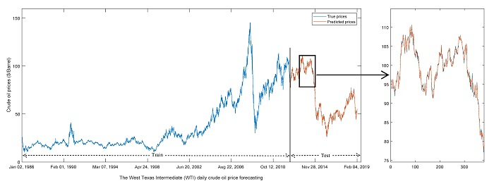
Crude oil is one of the leading types of energy that has great impacts on the global economy. Trying to accurately expect changes in crude oil prices benefits the producers and consumers of crude oil. However, the prices are affected by many factors, such as climate, exchange rate, supply and demand, speculation activities, geopolitics and so on, and they have fluctuated drastically in the last decades [1,2]. For example, the prices of West Texas Intermediate (WTI) reached over 145 USD/barrel in July 2008 and then quickly reduced to about 30 USD/barrel in the next five months. Crude oil prices have shown significant nonlinearity and nonstationarity in the last three decades. The complex fluctuation of crude oil prices makes it a very challenging task to accurately predict crude oil prices. Despite this, many researchers have contributed to building automatic models to forecast crude oil prices accurately.
The task of forecasting crude oil prices is to expect future prices using existing data. From the perspective of the input of the forecasting task, it can be divided into two groups: multivariate forecasting and univariate forecasting. The former usually feeds the data associated with types of variables, such as macroeconomic variables, exchange rates, sentiment analysis, inventory variables, previous crude oil prices, and so on, to the predictors [1,2,3,4,5,6,7], while the latter uses the previous prices only [8,9,10,11,12]. These are two different perspectives for studying crude oil price forecasting. In practical applications, the former is usually used to forecast long-term crude oil prices, for example, monthly prices or weekly prices, while the latter is for daily prices in most cases. In the task of forecasting crude oil prices, the predictors can be mainly categorized into two classes: statistical models (econometric models) and artificial intelligence (AI) models. Mirmirani and Li employed vector auto-regression (VAR) to forecast the movements of U.S. oil prices [13]. Murat and Tokat found that a vector error correction model (VECM) with crack spread futures outperformed the traditional random walk (RW) model [14]. Moshiri and Foroutan applied auto-regressive integrated moving average (ARIMA) and another statistical model, generalized autoregressive conditional heteroskedasticity (GARCH), to forecasting daily crude oil futures prices [15]. Some extensions of GARCH have also been employed in recent years [16,17,18]. In Lyocsa and Molnar’s study, the authors investigated whether the heterogeneous autoregressive (HAR) model can improve the results of forecasting the volatility of crude oil prices by using information from related energy commodity, and the experimental results demonstrated that such information can not improve the volatility forecasting [19]. Lv studied the performance of the HAR model of realized volatility (HAR-RV) for forecasting crude oil futures price volatility [20]. Naser found that the dynamic model averaging (DMA) model showed better performance in forecasting crude oil prices than all the other alternative models, and it could also achieve better results of forecasting spot prices than futures prices [21]. Azevedo and Campos combined ARIMA, exponential smoothing, and dynamic regression to forecast WTI and Brent crude oil spot prices, and the experimental results indicated that the combined model was promising for crude oil price forecasting [22].
The statistical models are usually built on the assumption of linearity and stationarity of the predicted time series. However, most research has shown that crude oil prices are highly nonlinear and nonstationary [8,12,23], so such characteristics limit the accuracy of statistical models for forecasting crude oil prices. To cope with the complex characteristics of crude oil prices, more and more scholars use AI models to forecast crude oil prices. The most popular AI models include artificial neural network (ANN) [12,24,25,26,27], support vector regression (SVR) [28,29] and least squares SVR (LSSVR) [2,10,30], sparse Bayesian learning (SBL) [31,32], extreme learning machine (ELM) [23,33,34], extreme gradient boosting (XGBoost) [8], random vector functional link (RVFL) network [11], long short-term memory (LSTM) [35], and so on. Yu et al. used a feed-forward neural network (FNN) to forecast each decomposed component from the raw series of crude oil prices, and then integrated the results of all components as the final forecasting result by an adaptive linear neural network (ALNN) [12]. Xiong et al. also used FNN to conduct multi-step-ahead weekly crude oil spot price forecasting [25]. Barunik and Malinska found that a focused time-delay NN could achieve higher accuracy than the compared models when forecasting monthly crude oil prices [26]. Extensive research has demonstrated that the kernel-based methods, such as SVR, LSSVR and relevance vector machine, are promising for forecasting crude oil prices [2,10,28,29,30,36]. Very recently, the LSTM, an artificial recurrent NN architecture widely used in deep learning, has been applied to forecasting crude oil prices. Owing to its power in processing sequences of data, the LSTM-based approach has yielded very promising forecasting results [35]. Chiroma et al. presented an extensive review of the research that applied AI-based models to crude oil price forecasting [37].
Due to the nonlinearity and nonstationarity of crude oil price series, statistical models and AI models usually cannot achieve satisfactory results by conducting forecasting with the raw crude oil prices directly. A simple but effective way is to adopt the “divide and conquer” strategy, that is, to decompose the complex signal into several relatively simple components and then extract relevant features or handle each component for further work. Typical applications of such strategy include fault diagnosis [38,39], biosignal analysis [40,41], time series forecasting [42,43], and so on [44,45,46]. Following this strategy, a “decomposition and ensemble” framework has become very popular in the field of energy forecasting, such as wind speed forecasting [47,48], load forecasting [49,50,51] and price forecasting [8,11,52,53] in recent years. Ren et al. integrated empirical mode decomposition (EMD) and SVR to forecast wind speed. Specifically, EMD was used to decompose the raw wind speed series into a couple of components (a residue and a few intrinsic mode functions (IMFs)). After that, SVR was used to build an individual forecasting model for each component. At last, the predicted values of all the components were aggregated as the final forecasting result [47]. Similarly, Li et al. utilized an extended EMD, namely, ensemble EMD (EEMD), and random forests (RF) for electricity consumption forecasting [31], and Yang and Wang applied complementary EEMD (CEEMD) and back propagation NN (BPNN) to forecast wind speed [54]. All the research indicates that the approaches following the framework of “decomposition and ensemble” is capable of significantly improving the accuracy of energy forecasting.
Regarding the decomposition methods, although EMD, EEMD and CEEMD have the ability of improving accuracy, they may introduce new noise into the recovered signal and still suffer from the “mode mixing” problem [55,56]. To solve this problem, a complete EEMD with adaptive noise (CEEMDAN) and an improved CEEMDAN (ICEEMDAN) were proposed [57,58]. The existing study has demonstrated the power of CEEMDAN/ICEEMDAN in energy forecasting [8,59]. As far as the forecasting method for each component, so-called individual forecasting, any regression methods can be selected for this purpose in theory. Besides the above-mentioned methods such as SVR, ANN, ELM, LSTM and so on, ridge regression (RR) is a simple but powerful regression for forecasting. Moreover, the accuracy of regression can be further improved by introducing kernels into RR (KRR), and the KRR has been successfully applied in wind speed forecasting [60,61], object tracking [62], and preheat temperature prediction [63]. The basic idea of the kernel trick is to map the features of the low-dimensional space to the high-dimensional space to obtain more representative features. Naik et al. used wavelet kernel RR and low rank multi-kernel RR to forecast the components of wind speed and wind power decomposed by EMD and variational mode decomposition (VMD), respectively [61,64]. The low rank multi-kernel RR in their approach was a simple linear combination by a polynomial kernel and a wavelet kernel, that is to say, the multi-kernel was actually a combination of two simple kernels [64]. The number and type of kernels may limit the performance of the proposed approach. Qian et al. used multi-kernel RR for object tracking, where the final kernel included one linear kernel, five polynomial kernels and five Gaussian kernels, and the parameter of each kernel was specified in advance and the optimization process was only to optimize the weight of each kernel [62]. Regarding multi-kernel learning, an ideal way is to optimize the weights and the parameters of each kernel together. The nature-inspired algorithms, such as particle swarm optimization (PSO) [65,66,67], differential evolution (DE) [68,69], ant colony optimization [70,71] and so on, can be applied to optimizing both the weights and the parameters of the multi-kernel learning. Among the algorithms, DE has proven to be very powerful for numerical optimization.
Motivated by the potential of ICEEMDAN in signal decomposition, RR in regression and DE in numerical optimization, we proposed a novel approach integrating ICEEMDAN, DE and RR, namely, ICEEMDAN-DE-RR, for crude oil price forecasting in this paper. Specifically, the ICEEMDAN-DE-RR consists of three steps. First, ICEEMDAN is employed to decompose the raw daily crude oil price series into several relatively simple components. Second, we use RR or KRR optimized by DE to forecast each component individually. Finally, the predicted results from each component are aggregated as the final forecasting result.
The main contributions of this paper lie in the following:
- (1)
- We propose a new framework of multiple kernel learning, which simultaneously optimizes the weights and parameters of kernels using nature-inspired optimization.
- (2)
- We forecast crude oil prices by integrating ICEEMDAN, DE and RR, following the “decomposition and ensemble” framework. To the best of our knowledge, it is the first time that this combination is used for forecasting tasks.
- (3)
- The experimental results indicate that the proposed approach is effective for crude oil price forecasting.
It is worth pointing out that although there have existed lots of models following the “decomposition and ensemble” framework for energy forecasting, the proposed models are different from them in several aspects. First, it is an attempt to use RR to forecast crude oil prices for the first time. Existing research focuses on using RR to forecast wind speed, hydrologic time series, real estate appraisal and so on [60,72,73], not including crude oil prices. Second, a new multiple kernel learning framework is proposed using DE to optimize the parameters and/or weight of each base kernel, as well as the regularization item simultaneously. The experimental results demonstrate the effectiveness of the proposed approach. Third, the integration of ICEEMDAN, DE and RR is used to forecast time series for the first time.
The novelty of this paper is three-fold: (1) Based on the power of ICEEMDAN, DE, and RR in signal decomposition, numerical optimization, and regression, respectively, a novel combination of these three methods is proposed for time series forecasting; (2) To improve the representability of kernels, a novel multiple kernel learning framework using DE to simultaneously optimize the weights and parameters of every single kernel is proposed, which can be applied to both classification and regression; (3) The proposed ICEEMDAN-DE-RR approaches are firstly applied to forecasting crude oil prices and the results demonstrate the effectiveness of the approaches.
The remainder of this paper is structured as follows. In Section 2, we briefly introduce ICEEMDAN, DE and RR. Section 3 formulates the proposed ICEEMDAN-DE-RR method in detail. To evaluate the proposed ICEEMDAN-DE-RR, we report and analyze the experimental results in Section 4. Finally, we conclude the paper in Section 5.
2. Methods
2.1. Improved Complete Ensemble Empirical Mode Decomposition with Adaptive Noise (ICEEMDAN)
ICEEMDAN was originated from EMD proposed by Huang et al. [55,56,57,58]. EMD is an adaptive method for time-space analysis, which decomposes a raw sequence that is non-linear and non-stationary into several IMFs and one residue. The main steps of EMD are described as follows:
- Step 1:
- Find out all local extrema of the raw data ;
- Step 2:
- Link all local minima and local maxima to construct the lower envelopes and upper envelopes , respectively;
- Step 3:
- Compute the local mean, i.e., ;
- Step 4:
- Extract the first IMF and residue by and , respectively;
- Step 5:
- For , if find out more than two local extrema of , go back to step 2 and get and .
In EMD, it was found that there were similar parts of signals existing at the same corresponding position in different IMFs, which was called mode mixing. Because of it, IMFs have lost their physical meanings [55]. To cope with this issue, Wu and Huang proposed Ensemble EMD (EEMD) by performing EMD many times on the time series with added white noises [56]. The new time series with white noises can be formulated as Equation (1):
where represents the raw data series and is the i-th white noise, .
Then, when every is decomposed, we can get the corresponding . To compute the real k-th IMF, , EEMD calculates the average of the , which can remove the effect of the white noises. However, in practice, one of the limitations of EEMD is that the recovered signal will include residual noise. To solve this problem, Torres et al. proposed a new extension of EEMD, termed as CEEMDAN for signal decomposition [57]. For , the k-th IMF and residue can be computed as Equations (2) and (3):
where represents the first IMF decomposed from the series, and is used to set the signal-to-noise (SNR) at each stage.
In 2014, Colominas et al. found that the IMFs of CEEMDAN contained some residual noise and some “spurious” modes. Thus, they further proposed a method to improve CEEMDAN (ICEEMDAN) [57,58], whose main steps can be described as follows:
- Step 1:
- Add the first IMF of the given white noises to the original series , as shown in following:where is the level of noise.
- Step 2:
- Find out the local means of and calculate the average of local means to get the following residue:
- Step 3:
- Then, we can get the first IMF, as shown in Equation (6):
- Step 4:
In this paper, the ICEEMDAN is used to decompose the original data series into several IMFs and one residue, standing for local physical features of original signals. The difficult task of forecasting the original signals is now becoming several relatively simple sub-tasks.
2.2. Kernel Ridge Regression (KRR)
Ridge regression (RR) is a typical linear regression that uses a sum-of-squares error function and regularization technique to control the bias variance trade-off, whose purpose is to discover the linear structures hidden in the data [74]. Kernel ridge regression (KRR) is an extension of RR by introducing a kernel function that maps the input data in a low dimensional space to a high one. The kernel function k is defined on an input space and is with the formula: . The kernel function is actually a feature map from d dimensional space into a high-dimensional Hilbert Space , such that [75,76,77]. The most popular kernel functions include:
- Linear kernel: .
- Polynomial kernel: , where a, b, and c are the coefficient, constant and degree of , respectively.
- Sigmoid kernel: , where d and e are the coefficient and constant, respectively.
- Radial basis function (RBF) kernel: , where f is related to the width of the kernel.
With the kernel functions and n data samples ( is the target value of corresponding , ), we can construct the kernel matrix as Equation (9):
Then the KRR problem can be formulated as Equation (10):
where is the target vector of all the n data samples, w is the unknown vector to be found, and is a regularization item to avoid a large range of w. The solution in terms of w can be easily given in a closed-from manner as Equation (11):
where is an identity matrix with ones on the main diagonal and zeros elsewhere.
Kernel types and parameters are two important factors for KRR. Some existing research used only a single kernel with specified parameters or simple combinations of several kernels with a fixed weight of every kernel in practical problems, limiting the forecasting performance of KRR. To improve the performance, an ideal solution is to adaptively optimize the weight and/or the parameters of each single kernel using some nature-inspired optimization algorithms. In this paper, we use differential evolution (DE) to optimize such weights and/or parameters for kernels.
2.3. Differential Evolution (DE)
Differential evolution (DE) is a member of the family of nature-inspired algorithms, and it has been demonstrated that DE is very powerful in solving various science and engineering problems [68]. The main idea of DE is to optimize a problem by using a few operations to iteratively improve a set of candidate solutions with evaluation criteria. Basically, the evolutionary process of DE consists of four stages/operations: initialization, mutation, crossover, and selection.
2.3.1. Initialization
For a D-dimensional optimization problem, given the population size P, evolutionary generation G, and the lower and upper bounds of each decision variable and respectively, the -th decision variable of the -th individual can be initialized as Equation (12):
where the “1” at the right-up corner of I represents the current evolutionary generation, and generates a random real number between 0 and 1.
The initialization produces a population with P individuals/solutions/vectors, and the -th decision variable in each individual is in the range of .
2.3.2. Mutation
The purpose of mutation is to generate a new vector , so-called mutant vector, from several existing vectors/individuals with respect to each vector , so-called target vector, in the population of the -th generation. Some popular mutation strategies are shown as follows:
where are mutually random indices of the individuals, F is a preset parameter for scaling the difference vector, and is the best individual at the -th generation.
2.3.3. Crossover
The purpose of crossover is to generate a trial vector from the target vector and its corresponding mutant vector with the following strategy:
where is a user-defined crossover rate that satisfies , and is a random integer in to ensure that at least one decision variable in can be passed to directly.
2.3.4. Selection
The selection operation is to select the better vector from the target vector and its corresponding trial vector for the next generation with evaluation by fitness function f. The selection strategy is mathematically shown in Equation (18):
3. The Proposed ICEEMDAN-DE-RR Approach
3.1. Ridge Regression by DE
For any types of RR, the regularization item is an important parameter to be optimized. Kernel is a very powerful trick in machine learning, which maps the data that are linearly inseparable in the input space into a higher dimensional space where the mapped data are linearly separable using kernel functions. Regarding kernel Ridge regression (KRR), besides the regularization item in Equation (10), the parameters for the single kernels , and need to be optimized. To further explore the ability of multiple kernel RR (MKRR) for crude oil price forecasting, we build a multiple kernel that consists of one , one , one and n s, as shown in Equation (19),
where are the weights of each single kernel, and and are parameters for each single kernel.
In our approach, we use DE to optimize the regularization item in RR, and for each single kernel, and , weights and for , respectively. The weights for , , are generated from real values optimized by DE to meet by Equation (20):
3.2. The Proposed ICEEMDAN-DE-RR Approach
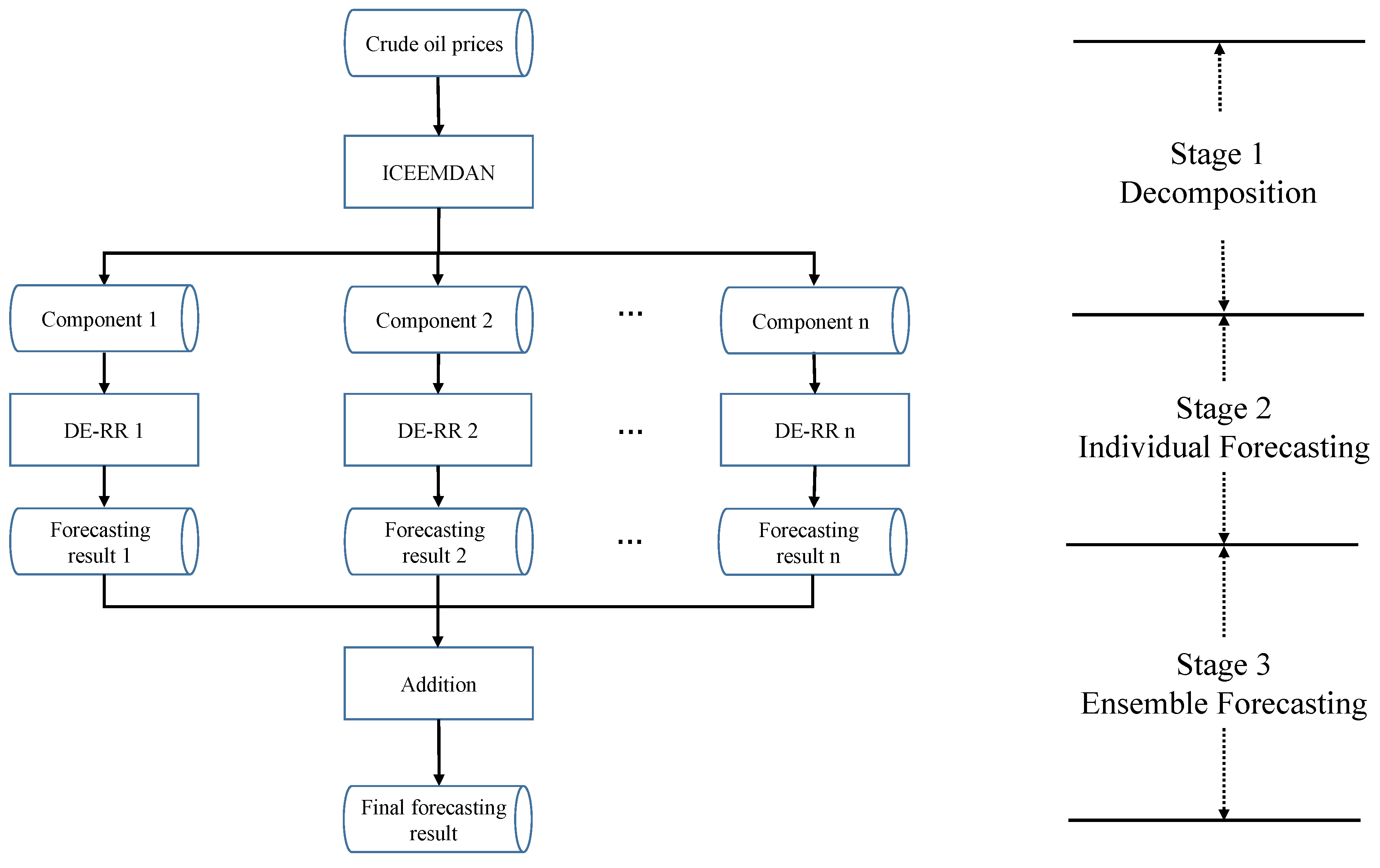
The proposed ICEEMDAN-DE-RR approach is a typical form of “decomposition and ensemble”, which consists of three stages, i.e., decomposition, individual forecasting, and ensemble forecasting, as shown in Figure 1.
The details of each stage are as follows:
- Stage 1:
- Decomposition. The daily raw crude oil price series is decomposed into two groups of components: several IMFs and one residue.
- Stage 2:
- Individual forecasting. The data samples in each component are divided into training set, validation set, and test set. The training set and validation set are used to build RR models, and then the test set is applied to evaluate the models. For each model, we use DE to optimize the regularization item, corresponding kernel parameters, and possible weights.
- Stage 3:
- Ensemble forecasting. The individual forecasting results of all the components in Stage 2 are aggregated as the final forecasting results by addition.
The proposed ICEEMDAN-DE-RR adopts the typical “divide-and-conquer” strategy, which divides the complexly non-linear and non-stationary crude oil prices into several relatively simple components and then handles each component with a relatively simple DE-based RR predictor. With the strategy, the tough task of forecasting raw crude oil price series becomes several relatively simple sub-tasks of forecasting each component.
It is worth pointing out that although there is a lot of work on energy forecasting following the framework of “decomposition and ensemble”, our proposed work is very different from the work in several aspects: (1) RR and KRR are first applied to crude oil forecasting; (2) a novel multiple kernel RR (MKRR) optimized by DE is proposed and it can be applied in other fields; and (3) the ICEEMDAN, DE and RR are integrated to forecast daily crude oil prices for the first time.
4. Experimental Results and Comparative Analysis
4.1. Data Description
To validate the effectiveness of the proposed approach, we select the West Texas Intermediate (WTI) daily crude oil spot closing prices from 2 January 1986 to 4 February 2019 as an experimental dataset. There are 8342 samples in total, and the daily crude oil prices from 2 January 1986 to 14 June 2012, with 6673 samples accounting for 80% of the total samples, are chosen as the training set, while the rest are for testing. Within the training set, 5338 (80%) and 1335 (20%) samples are used for training and validation, respectively.
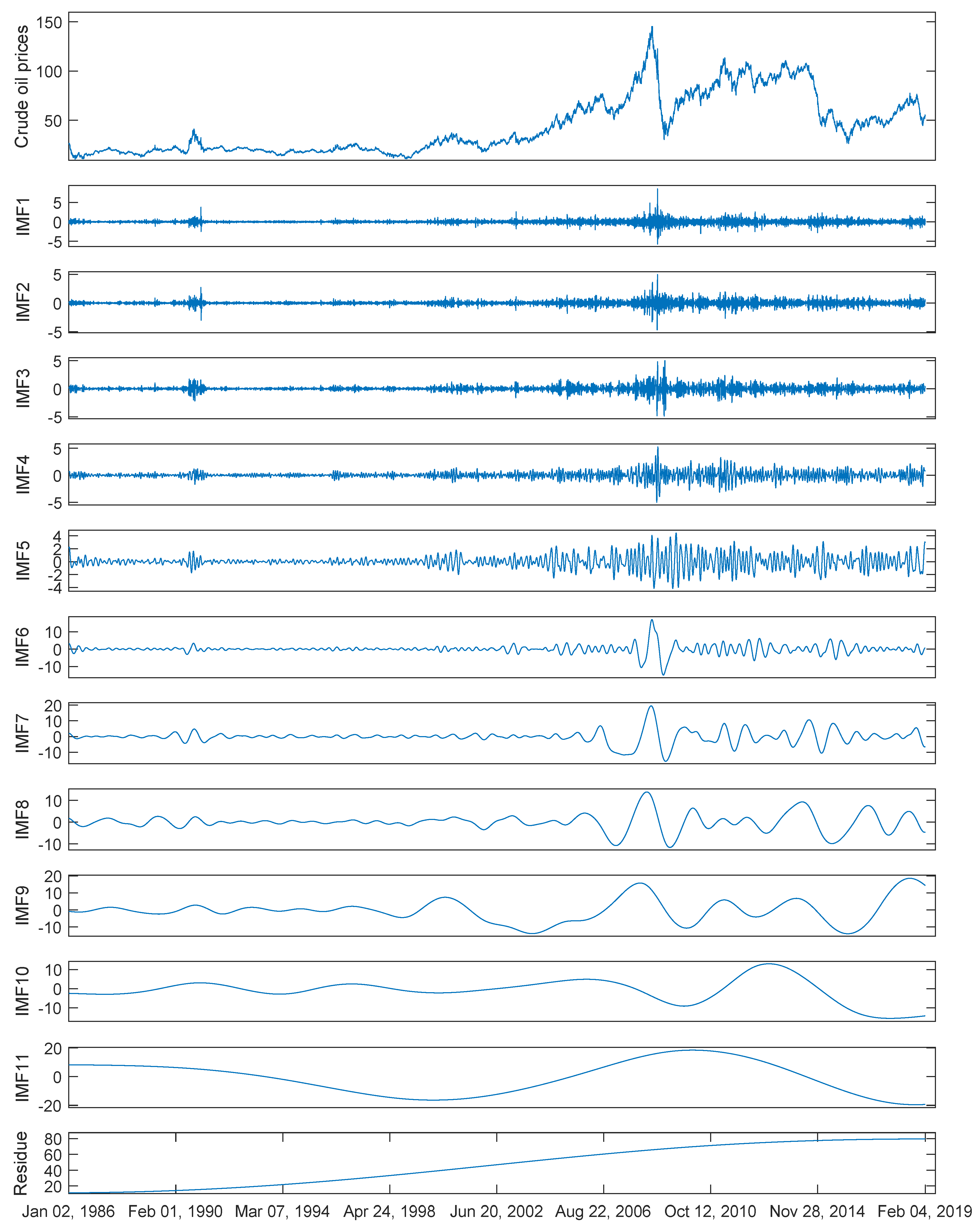
The WTI daily crude oil spot prices and corresponding decomposed components by ICEEMDAN are shown in Figure 2. We can see that the complex raw crude oil prices are decomposed into two groups: high-frequency group (IMF1-IMF5) and low-frequency group (IMF6-IMF11 and residue). The high-frequency components fluctuate within a narrow range of amplitude while the low-frequency ones fluctuate within a wide range of amplitude, making forecasting crude oil prices with the components easier than with the raw crude oil prices.
We conduct several types of multi-step-ahead forecasting with a lag of L in the experiments. A type of m-step-ahead prediction means forecasting the crude oil prices on the -th day with the L price samples before the t-th day but including the t-th day.
For a fair comparison, each decomposed component is scaled to using the min-max normalization, as formulated by Equation (21).
where and are crude oil price series before and after normalization respectively, and and are the maximum value and the minimum value of the time series, respectively.
4.2. Evaluation Criteria
We use a set of criteria to evaluate the proposed approach as well as the compared models. Specifically, the selected criteria include the mean absolute percent error (MAPE), the root-mean-square error (RMSE), and the directional statistic (Dstat). The MAPE, RMSE and Dstat are defined as Equations (22)–(24):
where and are the actual and predicted values at time t respectively, N is the size of the prediction, and if ; otherwise . The smaller the values of MAPE and RMSE, the better the model. In contrast, a higher Dstat means a better forecasting model.
Besides, we take the Diebold–Mariano (DM) test to compare the statistic difference of the accuracy of prediction between pairs of models. At first, we compute the difference of the prediction of pairs of models at time t as Equation (25):
where is the prediction of model a at time t and is the prediction of model b at time t. Then, the DM statistic can be defined as Equation (26):
where
where is a covariance matrix.
If the value of the DM test is negative and statistically significant (e.g., p-value ), it is proven that there is a significant difference between the predictive accuracy of pairs of models [78].
4.3. Experimental Settings
We forecast daily crude oil prices from the raw price series and decomposed components, so-called single models and ensemble models, respectively. As for single models, we compare the RR-based methods (RR, LinRR, PolyRR, SigRR, RbfRR and MKRR in Table 1) with two state-of-the-art AI models: LSSVR and BPNN, as well as two classical statistical methods: ARIMA and RW. Regarding ensemble models, we compare ICEEMDAN with EEMD to show the power of decomposition, and all the forecasting methods with single models except for ARIMA are applied to ensemble models. The parameters in the experiments are shown in detail in Table 1. Note that for the MKRR, we use 23 single kernels, i.e., one linear kernel, one polynomial kernel, one Sigmoid kernel and 20 RBF kernels, to build the multiple kernel, and both the weight and parameters of each single kernel are optimized by DE. The values or the ranges of some parameters are from existing literature [8,31]. In addition, we use RMSE as the fitness function to evaluate the individuals in DE.
All the experiments were performed by Matlab R2016b on a PC with 64-bit Windows 10, a 3.6 GHz i7 CPU and 32 GB RAM.
4.4. Results and Analysis
4.4.1. Single Models
The single models are performed on the raw daily crude oil prices directly. We compared the RR-based methods with LSSVR, BPNN and ARIMA. The experimental results are reported in Table 2, with the best and the worst results being shown in bold and underline, respectively, in terms of each criterion with each horizon.
From the table, we can find that the AI models outperform the statistical models in 6 out of 9 cases. Among the AI models, BPNN obtains two worst results: the MAPE value of 0.0161 as well as the RMSE value of 1.3050 with Horizon 1, while LSSVR and PolyRR obtain the worst values once: the Dstat value of 0.4592 and 0.4862 with Horizon 3 and 6, respectively. Overall, the RR-based single models outperform other models in most cases. In particular, RR achieves the best results in 6 out of 9 cases, showing that it is superior to other single models. Regarding the statistical models, RW is very close to but slightly better than ARIMA. In terms of MAPE and RMSE, for each model, the results become worse and worse when the horizon increases.
Regarding directional statistics, RbfRR, MKRR and BPNN achieve the highest values of 0.5186, 0.5090 and 0.4976 with Horizon 1, 3, and 6, respectively. In contrast, ARIMA and PolyRR obtain the worst values of 0.4868 and 0.4862 with Horizon 1 and 6, respectively. For Horizon 3, both LSSVR and RW obtain the worst Dstat values of 0.4952. The intervals of the best values and the corresponding worst values are so narrow that all the results of all cases are around 0.5, just like the result of random guessing, showing that it is a tough task to forecast the direction using single models.
To further compare the single models, we report the DM test results in Table 3, with the statistics and the corresponding p-values (in brackets). From this table, we have some findings. First, compared with the statistical model ARIMA and RW, the statistics of all the AI models in all cases except for BPNN with Horizon 1 are far below −2.000 and the corresponding p-values are much less than 0.01, indicating that the AI models significantly outperform ARIMA and RW. ARIMA and RW have very similar results. Second, LSSVM and BPNN underperform RR-based approaches in most cases, showing that the RR-based predictors are more effective than the statistical AI models (LSSVM and BPNN) for forecasting raw crude oil prices, to some extent. Third, as for RR-based models, the RR, PolyRR and MKRR have very close performance, which are superior to LinRR, SigRR and RbfRR. All the findings confirm the analysis on MAPE, RMSE and Dstat.
Due to the nonlinearity and nonstationarity, the performance of directly forecasting on raw crude oil price series needs to be improved. To cope with this issue, we use ICEEMDAN to decompose the raw series into several components each of which shows relatively simple characteristics when compared with the raw series, and then each component is predicted using an AI model individually. At last, the predicted results of all components are aggregated as the final result.
4.4.2. Ensemble Models
To demonstrate the effectiveness of ICEEMDAN, we also use EEMD as one of the decomposition methods for comparison. For the forecasting methods, we compare RR-base predictors with two state-of-the-art AI methods: LSSVR and BPNN. The values of MAPE, RMSE and Dstat with ensemble models are shown in Table 4.
As far as MAPE and RMSE with EEMD are concerned, the results of different forecasting models except for BPNN and RW are significantly superior to those of the corresponding single models. For example, the best (lowest) MAPE, and RMSE with Horizon 1 are improved from 0.0154 to 0.0084, and from 1.2454 to 0.6399, respectively. Regarding Dstat, the best/worst value except those by RW is 0.8231/0.7344, which is far greater than the values of single models. Among the forecasting methods, RR-based predictors achieve all the best values while BPNN and RW obtain all the worst results. Specifically, RR, SigRR and PolyRR achieve the best values 4, 4 and 3 out of 9 times, respectively. Except for the values of MAPE and RMSE with Horizon 1, the ensemble models by BPNN are advantageous over single BPNN. Another finding is that RW obtains the worst values 8 out of 9 times. In particular, the Dstat values by RW are always around 0.5, and the possible reason is that RW performs poorly in forecasting high-frequency components. The experimental results indicate that the ensemble models except for RW can significantly improve the forecasting effectiveness when compared with the single models.
When we look at the results with ICEEMDAN and AI models in Table 4, we can see a significant improvement in the forecasting ability. As for MAPE, the value of each model with ICEEMDAN is superior to that of its competitor with EEMD. Specifically, RR achieves the best (lowest) MAPE for all the horizons, while BPNN obtains the worst values for the same horizons. For Horizon 1, PolyRR, SigRR and MKRR also achieve the best MAPE (0.0043) as RR does. The results of RMSE show similar characteristics that all the models with ICEEMDAN exceed those with EEMD. The best values of RMSE with Horizon 1, 3, and 6 are achieved by SigRR, RR, and RR, respectively. In contrast, LinRR, LinRR and BPNN obtain the worst RMSEs with Horizon 1, 3 and 6, respectively. It is worth pointing out that the directional statistics is significantly improved by ICEEMDAN. The best Dstat (0.9113) is achieved by SigRR with Horizon 1, and the other models achieve very close Dstat, indicating that this metric is very stable with ICEEMDAN. The worst (lowest) value of Dstat is 0.6661, which is much higher than the best one by single models (0.5186). Therefore, the models with ICEEMDAN and AI models are able to effectively improve the results of directional statistics. Regarding the results with ICEEMDAN and RW models, they still perform poorly and obtain the nine worst values, although RW models with ICEEMDAN perform slightly better than those with EEMD for Horizon 1 and 2.
For the models with both EEMD and ICEEMDAN, most results of MAPE, RMSE and Dstat will become worse when the horizon increases, showing that it is more difficult to forecast crude oil prices with a long horizon than with a short one.
We still apply the DM test to compare the ensemble models, and the results are shown in Table 5. From this table, we can see that when the forecasting methods with ICEEMDAN are compared with those with EEMD, the statistical values are far below zero and the p-value is very close to zero (usually less than 0.0001) with Horizon 1 and 3, indicating that the former significantly outperforms the latter with these two horizons. Regarding Horizon 6, the forecasting methods, except for BPNN with ICEEMDAN, still outperform the corresponding methods with EEMD. For each decomposition, the RR-based methods are usually superior to LSSVR and BPNN. Among the RR-based predictors, RR and SigRR have the best forecasting ability, followed by MKRR and PolyRR, while RbfRR and LinRR have a slightly worse predictive power. In addition, the models with AI are all superior to the corresponding models with RW, showing that the forecasting effectiveness does not stem from luck but by the forecasting superiority of the proposed approaches. All the DM test results confirm that ICEEMDAN and RR-based predictors are very effective for forecasting daily crude oil prices. The proposed approach that integrates ICEEMDAN and RR is capable of improving the results of crude oil price forecasting.
4.5. Discussion
In this subsection, we will discuss the impact of the parameter settings of the ICEEMDAN, the impact of the lag orders and the result of each individual component. Since the above results and analysis have shown that RR and SigRR usually outperform the other models, we will take both RR and SigRR as examples to discuss the following.
4.5.1. The Impact of the Parameter Settings of the ICEEMDAN
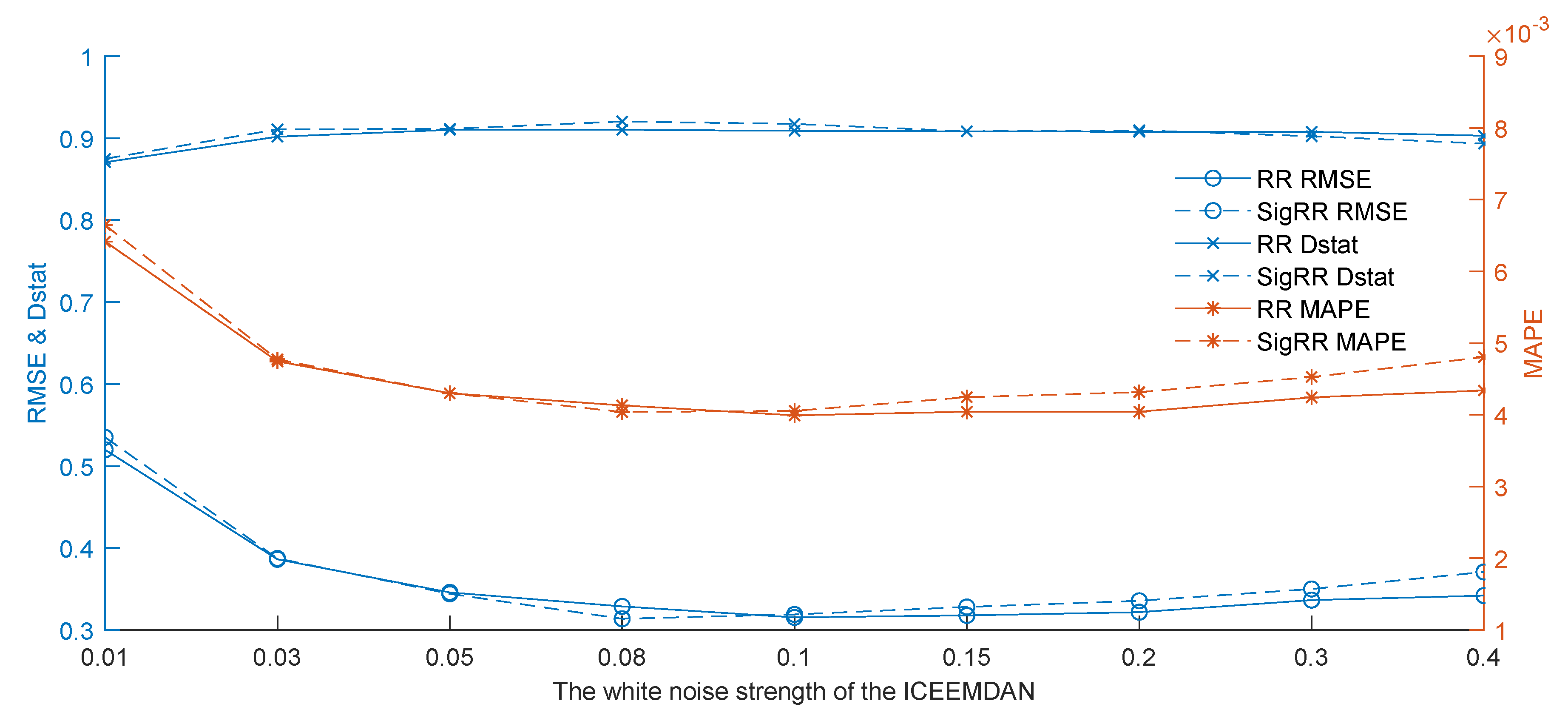
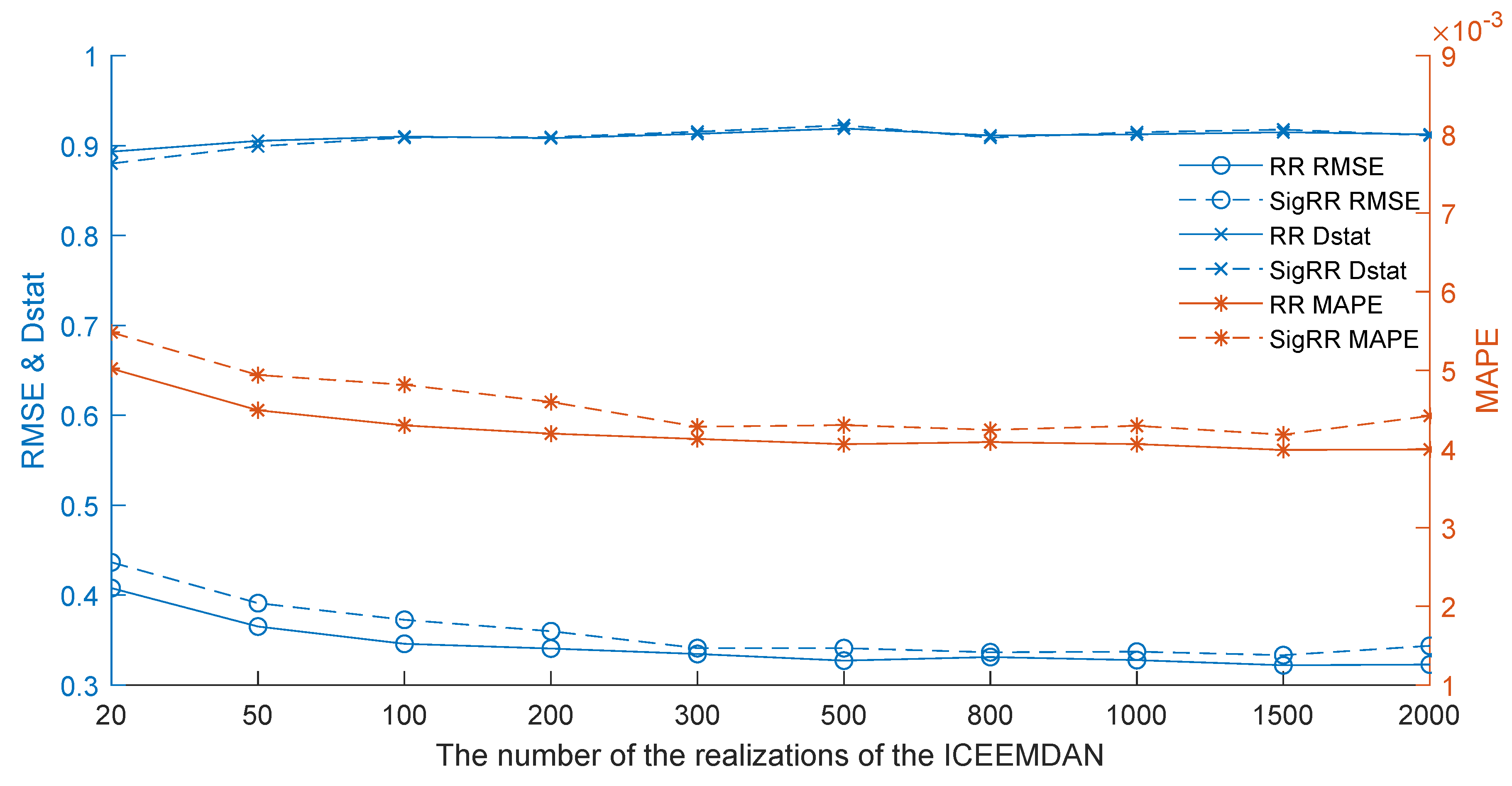
When we use the ICEEMDAN to decompose the daily crude oil price series, we need to add noises to the series and decompose the series many times. Therefore, the noise standard deviation and the number of realizations are two important parameters. To study the impact of on forecasting, we run the proposed approach with a variable in the range of {0.01, 0.03, 0.05, 0.08, 0.1, 0.15, 0.2, 0.3, 0.4} while fixing other parameters. The experimental results are shown in Figure 3. Likewise, we use a variable in the range of {20, 50, 100, 200, 300, 500, 800, 1000, 1500, 2000} and fixed other parameters to study the impact of the number of realizations, as shown in Figure 4.
It can be seen from Figure 3 that the results in terms of RMSE, MAPE and Dstat are gradually improved when increases from 0.01 to 0.08. In contrast, after that, all the evaluation indicators are getting worse and worse with the increase of noise strength when is greater than 0.1. Both RR and SigRR have similar trends, and one of the two models is alternatively better than the other. The results show that the white noise strength has great impact on the forecasting performance and an ideal white noise strength is between 0.05 and 0.1.
When we look at Figure 4, we can find that when the number of the realization is 20, the results of RMSE, MAPE and Dstat are all rather bad. When the number of realization increases from 20 to 500, all the results become better and better. Specifically, the Dstat reaches the best values for both RR and SigRR when the number of realization equals 500, while the results of RMSE and MAPE are very close to the best values. After that, the values of the three indicators are very stable when the number of realization varies from 500 to 2000. The results indicate that 500 is very ideal for the number of realizations.
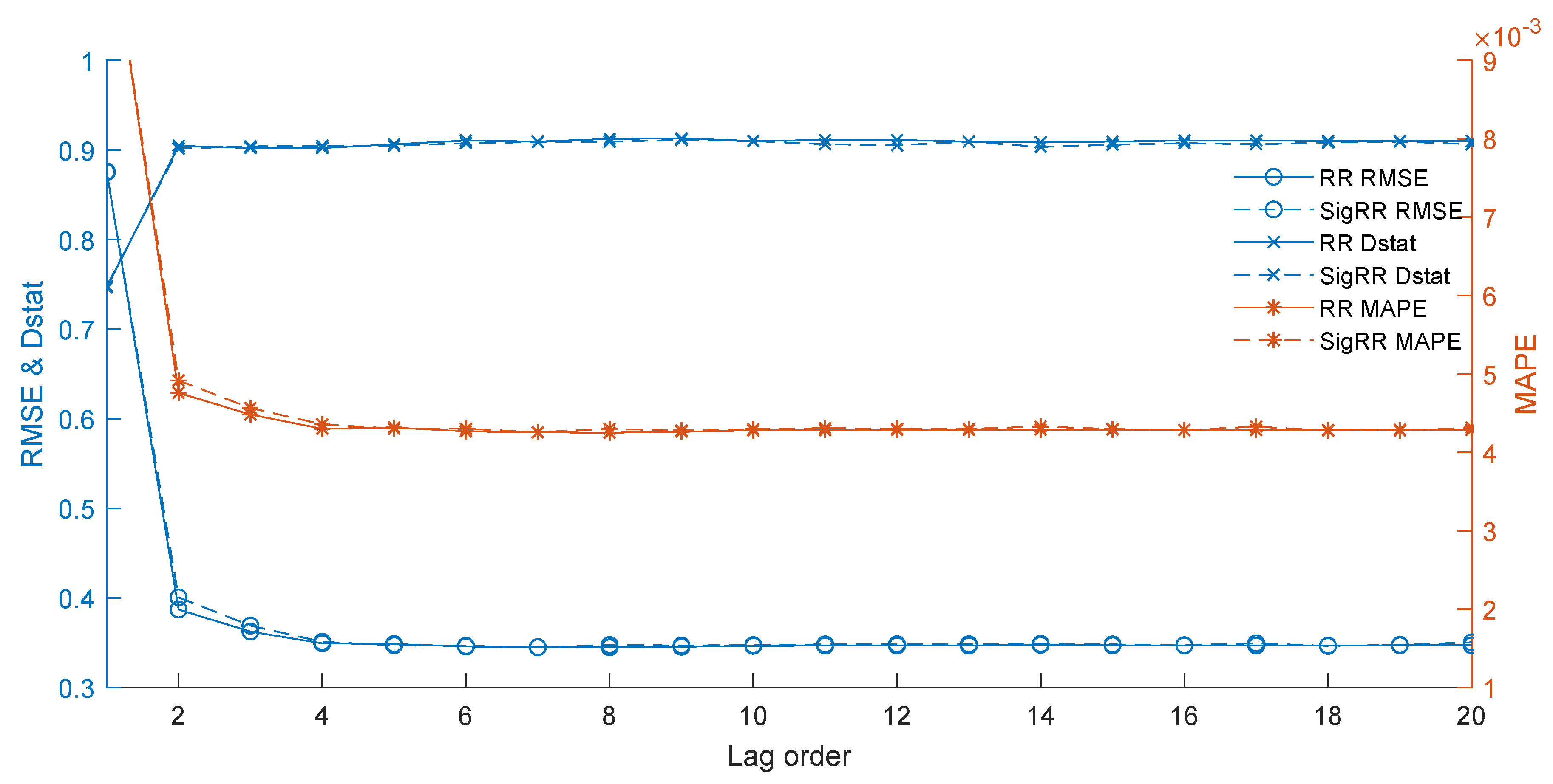
4.5.2. The Impact of the Lag Orders
Lag orders refer to the length of recent data points treated as explanatory variables to build time series models. We further investigate the impact of variable lag orders from 1 to 20 with horizon 1, and the results are shown in Figure 5. When the lag order is equal to 1, the results of the evaluation indicators are the worst. However, when it varies from 1 to 6, the corresponding results are all becoming better and better. After that, the results have remained almost unchanged for the lag order from 6 to 20. Therefore, the best lag order is 6 because it can provide satisfactory results with less input, which confirms the previous study [12,31].
4.5.3. The Result of Each Individual Component
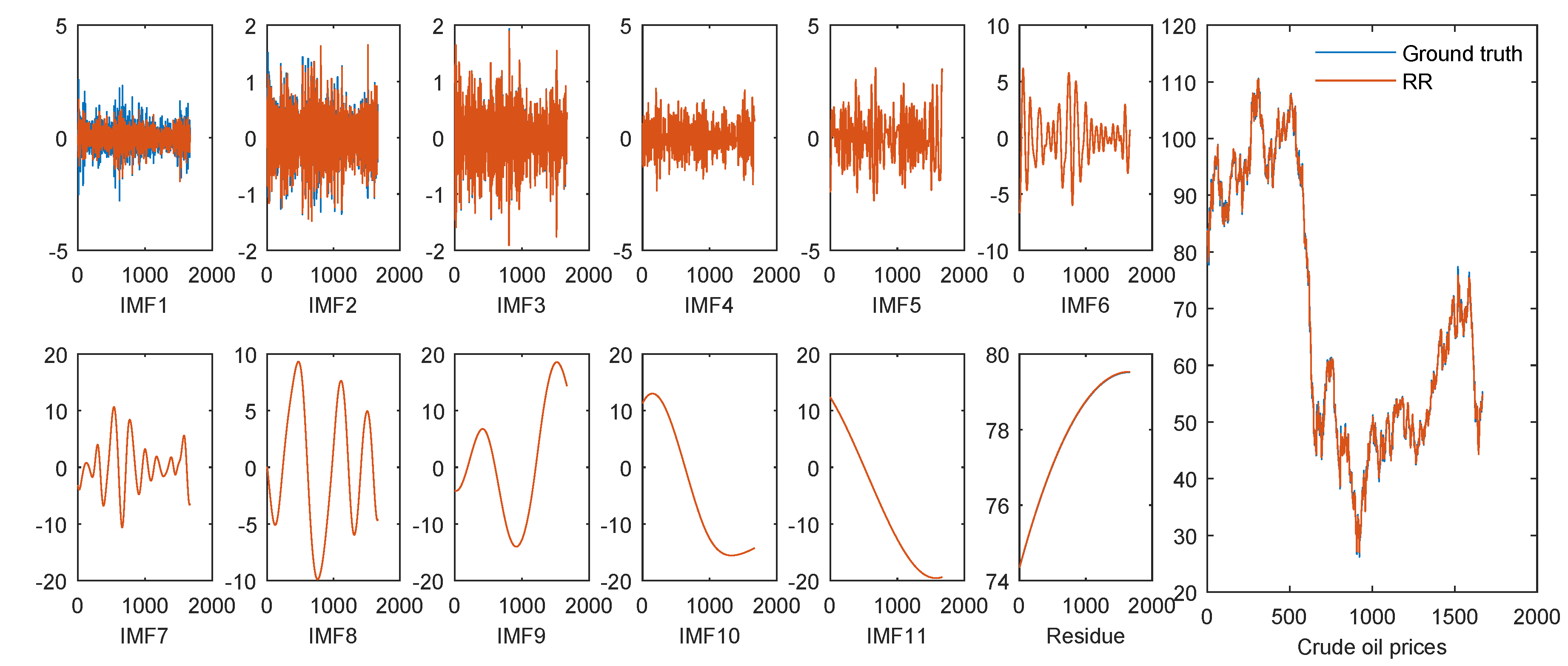
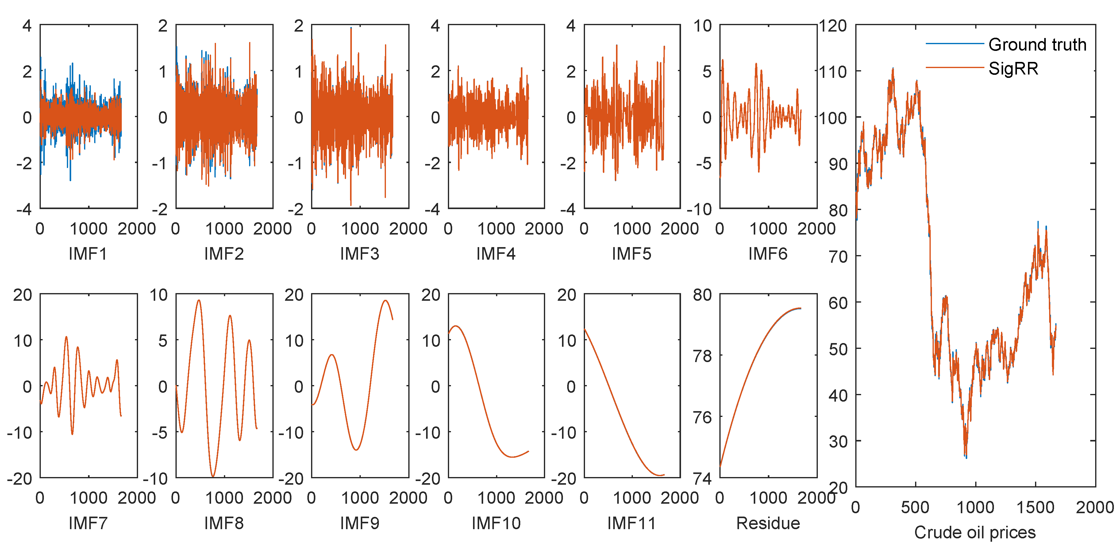
Each decomposed component by the ICEEMDAN shows either high-frequency or low-frequency characteristics. In general, it is harder to forecasting a high-frequency component than a low-frequency one. We plot the predicted values and raw data of each component and the raw crude oil prices by RR and sigRR in Figure 6 and Figure 7, respectively.
It can be seen from these figures that both RR and SigRR are able to forecast the high-frequency components (IMF6-IMF11 as well as the residue) very well, and the predicted errors mainly come from the high-frequency components (IMF1-IMF5), especially from IMF1. Since the volatility of the hight-frequency components is relatively narrow, the forecasting errors from such components might be restricted. This is one of the possible reasons why the framework of “decomposition and ensemble” is effective for time series forecasting.
5. Summary and Conclusions
Forecasting daily crude oil prices is an important but challenging task. To improve the forecasting performance, a series of approaches using ICEEMDAN, DE and RR, termed as ICEEMDAN-DE-RR, are proposed in this paper. The proposed approaches firstly use ICEEMDAN to decompose the complex original crude oil prices into several components, and then each component is forecasted individually by DE-based RR predictors. In the end, the sum of the predicted results of all the components is taken as the final result. The extensive experiments demonstrated the proposed approaches can outperform some state-of-the-art methods.
Especially from the experimental results, we have the following interesting findings: (1) It is a very difficult task to accurately forecast daily crude oil prices with the raw price series because of its nonlinearity and nonstationarity; (2) AI-models usually outperform statistical methods when forecasting crude oil prices; (3) RR-based predictors with DE optimizing the parameters have good forecasting ability; (4) The framework of “decomposition and ensemble” can significantly improve the performance of forecasting daily crude oil prices; ICEEMDAN is advantageous over EEMD for the forecasting tasks; (5) The proposed ICEEMDAN-DE-RR approach outperforms the competitive methods in terms of several evaluation metrics, indicating that it is promising for daily crude oil price forecasting. (6) Regarding RR-based predictors, RR and SigRR with DE optimizing parameters can achieve very promising forecasting results in terms of several criteria.
In the future, we will apply the proposed approaches to forecasting other types of energy time series, such as natural gas prices, wind speed, wind power and electricity load.
Author Contributions
Formal analysis, T.L. and X.L.; Funding acquisition, X.L.; Investigation, J.W. and T.H.; Methodology, T.L.; Resources, T.H.; Software, T.L. and Y.Z.; Supervision, T.L. and X.L.; Writing—original draft, T.L. and Y.Z.; Writing—review & editing, T.L. and Y.Z.
Funding
This work was supported by the Fundamental Research Funds for the Central Universities (Grant No. JBK1902029), the Ministry of Education of Humanities and Social Science Project (Grant No. 19YJAZH047), Sichuan Science and Technology Program (Grant No. 2019YFG0117) and the Scientific Research Fund of Sichuan Provincial Education Department (Grant No. 17ZB0433).
Conflicts of Interest
The authors declare no conflict of interest.
References
- Miao, H.; Ramchander, S.; Wang, T.; Yang, D. Influential factors in crude oil price forecasting. Energy Econ. 2017, 68, 77–88. [Google Scholar] [CrossRef]
- Naderi, M.; Khamehchi, E.; Karimi, B. Novel statistical forecasting models for crude oil price, gas price, and interest rate based on meta-heuristic bat algorithm. J. Pet. Sci. Eng. 2019, 172, 13–22. [Google Scholar] [CrossRef]
- Ye, M.; Zyren, J.; Shore, J. A monthly crude oil spot price forecasting model using relative inventories. Int. J. Forecast. 2005, 21, 491–501. [Google Scholar] [CrossRef]
- Movagharnejad, K.; Mehdizadeh, B.; Banihashemi, M.; Kordkheili, M.S. Forecasting the differences between various commercial oil prices in the Persian Gulf region by neural network. Energy 2011, 36, 3979–3984. [Google Scholar] [CrossRef]
- Zhang, Y.; Ma, F.; Shi, B.; Huang, D. Forecasting the prices of crude oil: An iterated combination approach. Energy Econ. 2018, 70, 472–483. [Google Scholar] [CrossRef]
- Wen, F.; Gong, X.; Cai, S. Forecasting the volatility of crude oil futures using HAR-type models with structural breaks. Energy Econ. 2016, 59, 400–413. [Google Scholar] [CrossRef]
- Li, J.; Zhu, S.; Wu, Q. Monthly crude oil spot price forecasting using variational mode decomposition. Energy Econ. 2019, 83, 240–253. [Google Scholar] [CrossRef]
- Zhou, Y.; Li, T.; Shi, J.; Qian, Z. A CEEMDAN and XGBOOST-Based Approach to Forecast Crude Oil Prices. Complexity 2019, 2019, 4392785. [Google Scholar] [CrossRef]
- He, K.; Yu, L.; Lai, K.K. Crude oil price analysis and forecasting using wavelet decomposed ensemble model. Energy 2012, 46, 564–574. [Google Scholar] [CrossRef]
- Yu, L.; Dai, W.; Tang, L.; Wu, J. A hybrid grid-GA-based LSSVR learning paradigm for crude oil price forecasting. Neural Comput. Appl. 2016, 27, 2193–2215. [Google Scholar] [CrossRef]
- Tang, L.; Wu, Y.; Yu, L. A non-iterative decomposition-ensemble learning paradigm using RVFL network for crude oil price forecasting. Appl. Soft. Comput. 2018, 70, 1097–1108. [Google Scholar] [CrossRef]
- Yu, L.; Wang, S.; Lai, K.K. Forecasting crude oil price with an EMD-based neural network ensemble learning paradigm. Energy Econ. 2008, 30, 2623–2635. [Google Scholar] [CrossRef]
- Mirmirani, S.; Li, H.C. A comparison of VAR and neural networks with genetic algorithm in forecasting price of oil. Appl. Artif. Intell. Financ. Econ. 2004, 19, 203–223. [Google Scholar]
- Murat, A.; Tokat, E. Forecasting oil price movements with crack spread futures. Energy Econ. 2009, 31, 85–90. [Google Scholar] [CrossRef]
- Moshiri, S.; Foroutan, F. Forecasting nonlinear crude oil futures prices. Energy J. 2006, 27, 81–95. [Google Scholar] [CrossRef]
- Herrera, A.M.; Hu, L.; Pastor, D. Forecasting crude oil price volatility. Int. J. Forecast. 2018, 34, 622–635. [Google Scholar] [CrossRef]
- Nademi, A.; Nademi, Y. Forecasting crude oil prices by a semiparametric Markov switching model: OPEC, WTI, and Brent cases. Energy Econ. 2018, 74, 757–766. [Google Scholar] [CrossRef]
- Zhang, Y.J.; Yao, T.; He, L.Y.; Ripple, R. Volatility forecasting of crude oil market: Can the regime switching GARCH model beat the single-regime GARCH models? Int. Rev. Econ. Financ. 2019, 59, 302–317. [Google Scholar] [CrossRef]
- Lyocsa, S.; Molnar, P. Exploiting dependence: Day-ahead volatility forecasting for crude oil and natural gas exchange-traded funds. Energy 2018, 155, 462–473. [Google Scholar] [CrossRef]
- Lv, W. Does the OVX matter for volatility forecasting? Evidence from the crude oil market. Phys. A 2018, 492, 916–922. [Google Scholar] [CrossRef]
- Naser, H. Estimating and forecasting the real prices of crude oil: A data rich model using a dynamic model averaging (DMA) approach. Energy Econ. 2016, 56, 75–87. [Google Scholar] [CrossRef]
- Azevedo, V.G.; Campos, L.M.S. Combination of forecasts for the price of crude oil on the spot market. Int. J. Prod. Res. 2016, 54, 5219–5235. [Google Scholar] [CrossRef]
- Tang, L.; Dai, W.; Yu, L. A Novel CEEMD-Based EELM Ensemble Learning Paradigm for Crude Oil Price Forecasting. Int. J. Inf. Technol. Decis. Mak. 2015, 14, 141–169. [Google Scholar] [CrossRef]
- Tehrani, R.; Khodayar, F. A hybrid optimized artificial intelligent model to forecast crude oil using genetic algorithm. Afr. J. Bus. Manag. 2011, 5, 13130–13135. [Google Scholar] [CrossRef]
- Xiong, T.; Bao, Y.; Hu, Z. Beyond one-step-ahead forecasting: Evaluation of alternative multi-step-ahead forecasting models for crude oil prices. Energy Econ. 2013, 40, 405–415. [Google Scholar] [CrossRef] [Green Version]
- Barunik, J.; Malinska, B. Forecasting the term structure of crude oil futures prices with neural networks. Appl. Energy 2016, 164, 366–379. [Google Scholar] [CrossRef] [Green Version]
- Ding, Y. A novel decompose-ensemble methodology with AIC-ANN approach for crude oil forecasting. Energy 2018, 154, 328–336. [Google Scholar] [CrossRef]
- Fan, L.; Pan, S.; Li, Z.; Li, H. An ICA-based support vector regression scheme for forecasting crude oil prices. Technol. Forecast. Soc. Chang. 2016, 112, 245–253. [Google Scholar] [CrossRef]
- Yu, L.; Zhang, X.; Wang, S. Assessing Potentiality of Support Vector Machine Method in Crude Oil Price Forecasting. Eurasia J. Math. Sci. Technol. Educ. 2017, 13, 7893–7904. [Google Scholar] [CrossRef]
- Zhang, Y.; Zhang, J. Volatility forecasting of crude oil market: A new hybrid method. J. Forecast. 2018, 37, 781–789. [Google Scholar] [CrossRef]
- Li, T.; Hu, Z.; Jia, Y.; Wu, J.; Zhou, Y. Forecasting Crude Oil Prices Using Ensemble Empirical Mode Decomposition and Sparse Bayesian Learning. Energies 2018, 11, 1882. [Google Scholar] [CrossRef]
- Wu, J.; Chen, Y.; Zhou, T.; Li, T. An Adaptive Hybrid Learning Paradigm Integrating CEEMD, ARIMA and SBL for Crude Oil Price Forecasting. Energies 2019, 12, 1239. [Google Scholar] [CrossRef]
- Yu, L.; Dai, W.; Tang, L. A novel decomposition ensemble model with extended extreme learning machine for crude oil price forecasting. Eng. Appl. Artif. Intell. 2016, 47, 110–121. [Google Scholar] [CrossRef]
- Wang, J.; Athanasopoulos, G.; Hyndman, R.J.; Wang, S. Crude oil price forecasting based on internet concern using an extreme learning machine. Int. J. Forecast. 2018, 34, 665–677. [Google Scholar] [CrossRef]
- Wu, Y.X.; Wu, Q.B.; Zhu, J.Q. Improved EEMD-based crude oil price forecasting using LSTM networks. Phys. A 2019, 516, 114–124. [Google Scholar] [CrossRef]
- Li, T.; Zhou, M.; Guo, C.; Luo, M.; Wu, J.; Pan, F.; Tao, Q.; He, T. Forecasting Crude Oil Price Using EEMD and RVM with Adaptive PSO-Based Kernels. Energies 2016, 9, 1014. [Google Scholar] [CrossRef]
- Chiroma, H.; Abdul-kareem, S.; Noor, A.S.M.; Abubakar, A.I.; Safa, N.S.; Shuib, L.; Hamza, M.F.; Gital, A.Y.; Herawan, T. A Review on Artificial Intelligence Methodologies for the Forecasting of Crude Oil Price. Intell. Autom. Soft Comput. 2016, 22, 449–462. [Google Scholar] [CrossRef]
- Deng, W.; Zhang, S.; Zhao, H.; Yang, X. A Novel Fault Diagnosis Method Based on Integrating Empirical Wavelet Transform and Fuzzy Entropy for Motor Bearing. IEEE Access 2018, 6, 35042–35056. [Google Scholar] [CrossRef]
- Zhao, H.; Yao, R.; Xu, L.; Yuan, Y.; Li, G.; Deng, W. Study on a Novel Fault Damage Degree Identification Method Using High-Order Differential Mathematical Morphology Gradient Spectrum Entropy. Entropy 2018, 20, 682. [Google Scholar] [CrossRef]
- Bajaj, V.; Pachori, R.B. Classification of Seizure and Nonseizure EEG Signals Using Empirical Mode Decomposition. IEEE Trans. Inf. Technol. Biomed. 2012, 16, 1135–1142. [Google Scholar] [CrossRef] [PubMed]
- Li, T.; Zhou, M. ECG Classification Using Wavelet Packet Entropy and Random Forests. Entropy 2016, 18, 285. [Google Scholar] [CrossRef]
- Zhang, H.; Wang, X.; Cao, J.; Tang, M.; Guo, Y. A multivariate short-term traffic flow forecasting method based on wavelet analysis and seasonal time series. Appl. Intell. 2018, 48, 3827–3838. [Google Scholar] [CrossRef]
- Pannakkong, W.; Sriboonchitta, S.; Huynh, V.N. An Ensemble Model of Arima and Ann with Restricted Boltzmann Machine Based on Decomposition of Discrete Wavelet Transform for Time Series Forecasting. J. Syst. Sci. Syst. Eng. 2018, 27, 690–708. [Google Scholar] [CrossRef]
- Li, T.; Yang, M.; Wu, J.; Jing, X. A novel image encryption algorithm based on a fractional-order hyperchaotic system and DNA computing. Complexity 2017, 2017, 9010251. [Google Scholar] [CrossRef]
- Li, T.; Shi, J.; Li, X.; Wu, J.; Pan, F. Image encryption based on pixel-level diffusion with dynamic filtering and DNA-level permutation with 3D Latin cubes. Entropy 2019, 21, 319. [Google Scholar] [CrossRef]
- Li, X.; Xie, Z.; Wu, J.; Li, T. Image encryption based on dynamic filtering and bit cuboid operations. Complexity 2019, 2019, 7485621. [Google Scholar] [CrossRef]
- Ren, Y.; Suganthan, P.N.; Srikanth, N. A Novel Empirical Mode Decomposition with Support Vector Regression for Wind Speed Forecasting. IEEE Trans. Neural Netw. Learn. Syst. 2016, 27, 1793–1798. [Google Scholar] [CrossRef] [PubMed]
- Yang, Z.S.; Wang, J. A combination forecasting approach applied in multistep wind speed forecasting based on a data processing strategy and an optimized artificial intelligence algorithm. Appl. Energy 2018, 230, 1108–1125. [Google Scholar] [CrossRef]
- Abdoos, A.; Hemmati, M.; Abdoos, A.A. Short term load forecasting using a hybrid intelligent method. Knowl.-Based Syst. 2015, 76, 139–147. [Google Scholar] [CrossRef]
- Fan, G.F.; Peng, L.L.; Hong, W.C.; Sun, F. Electric load forecasting by the SVR model with differential empirical mode decomposition and auto regression. Neurocomputing 2016, 173, 958–970. [Google Scholar] [CrossRef]
- Qiu, X.H.; Ren, Y.; Suganthan, P.N.; Amaratunga, G.A.J. Empirical Mode Decomposition based ensemble deep learning for load demand time series forecasting. Appl. Soft. Comput. 2017, 54, 246–255. [Google Scholar] [CrossRef]
- Sun, W.; Zhang, C.C. Analysis and forecasting of the carbon price using multi resolution singular value decomposition and extreme learning machine optimized by adaptive whale optimization algorithm. Appl. Energy 2018, 231, 1354–1371. [Google Scholar] [CrossRef]
- Wang, D.Y.; Luo, H.Y.; Grunder, O.; Lin, Y.B.; Guo, H.X. Multi-step ahead electricity price forecasting using a hybrid model based on two-layer decomposition technique and BP neural network optimized by firefly algorithm. Appl. Energy 2017, 190, 390–407. [Google Scholar] [CrossRef]
- Yang, Z.S.; Wang, J. A hybrid forecasting approach applied in wind speed forecasting based on a data processing strategy and an optimized artificial intelligence algorithm. Energy 2018, 160, 87–100. [Google Scholar] [CrossRef]
- Huang, N.E.; Shen, Z.; Long, S.R. A new view of nonlinear water waves: the Hilbert Spectrum 1. Annu. Rev. Fluid Mech. 1999, 31, 417–457. [Google Scholar] [CrossRef]
- Wu, Z.; Huang, N.E. Ensemble empirical mode decomposition: A noise-assisted data analysis method. Adv. Adapt. Data Anal 2009, 1, 1–41. [Google Scholar] [CrossRef]
- Torres, M.E.; Colominas, M.A.; Schlotthauer, G.; Flandrin, P. A complete ensemble empirical mode decomposition with adaptive noise. In Proceedings of the 2011 IEEE international conference on acoustics, speech and signal processing (ICASSP), Prague, Czech Republic, 22–27 May 2011; pp. 4144–4147. [Google Scholar]
- Colominas, M.A.; Schlotthauer, G.; Torres, M.E. Improved complete ensemble EMD: A suitable tool for biomedical signal processing. Biomed. Signal Process. Control 2014, 14, 19–29. [Google Scholar] [CrossRef]
- Dai, S.; Niu, D.; Li, Y. Daily peak load forecasting based on complete ensemble empirical mode decomposition with adaptive noise and support vector machine optimized by modified grey Wolf optimization algorithm. Energies 2018, 11, 163. [Google Scholar] [CrossRef]
- Douak, F.; Melgani, F.; Benoudjit, N. Kernel ridge regression with active learning for wind speed prediction. Appl. Energy 2013, 103, 328–340. [Google Scholar] [CrossRef]
- Naik, J.; Satapathy, P.; Dash, P.K. Short-term wind speed and wind power prediction using hybrid empirical mode decomposition and kernel ridge regression. Appl. Soft. Comput. 2018, 70, 1167–1188. [Google Scholar] [CrossRef]
- Qian, C.; Breckon, T.P.; Li, H. Robust visual tracking via speedup multiple kernel ridge regression. J. Electron. Imaging 2015, 24, 053016. [Google Scholar] [CrossRef] [Green Version]
- Maalouf, M.; Homouz, D.; Abutayeh, M. Accurate Prediction of Preheat Temperature in Solar Flash Desalination Systems Using Kernel Ridge Regression. J. Energy Eng. 2016, 142, E4015017. [Google Scholar] [CrossRef]
- Naik, J.; Bisoi, R.; Dash, P.K. Prediction interval forecasting of wind speed and wind power using modes decomposition based low rank multi-kernel ridge regression. Renew. Energy 2018, 129, 357–383. [Google Scholar] [CrossRef]
- Kennedy, J. Particle swarm optimization. In Encyclopedia of Machine Learning; Springer: Berlin, Germany, 2010; pp. 760–766. [Google Scholar]
- Deng, W.; Zhao, H.; Yang, X.; Xiong, J.; Sun, M.; Li, B. Study on an improved adaptive PSO algorithm for solving multi-objective gate assignment. Appl. Soft. Comput. 2017, 59, 288–302. [Google Scholar] [CrossRef]
- Deng, W.; Yao, R.; Zhao, H.; Yang, X.; Li, G. A novel intelligent diagnosis method using optimal LS-SVM with improved PSO algorithm. Soft Comput. 2019, 23, 2445–2462. [Google Scholar] [CrossRef]
- Storn, R.; Price, K. Differential evolution—A simple and efficient heuristic for global optimization over continuous spaces. J. Glob. Optim. 1997, 11, 341–359. [Google Scholar] [CrossRef]
- Das, S.; Suganthan, P.N. Differential Evolution: A Survey of the State-of-the-Art. IEEE Trans. Evol. Comput. 2011, 15, 4–31. [Google Scholar] [CrossRef]
- Dorigo, M.; Blum, C. Ant colony optimization theory: A survey. Theor. Comput. Sci. 2005, 344, 243–278. [Google Scholar] [CrossRef]
- Deng, W.; Xu, J.; Zhao, H. An Improved Ant Colony Optimization Algorithm Based on Hybrid Strategies for Scheduling problem. IEEE Access 2019, 20281–20292. [Google Scholar] [CrossRef]
- Yu, X.; Liong, S.Y. Forecasting of hydrologic time series with ridge regression in feature space. J. Hydrol. 2007, 332, 290–302. [Google Scholar] [CrossRef]
- Ahn, J.J.; Byun, H.W.; Oh, K.J.; Kim, T.Y. Using ridge regression with genetic algorithm to enhance real estate appraisal forecasting. Expert Syst. Appl. 2012, 39, 8369–8379. [Google Scholar] [CrossRef]
- Zhang, S.; Hu, Q.; Xie, Z.; Mi, J. Kernel ridge regression for general noise model with its application. Neurocomputing 2015, 149, 836–846. [Google Scholar] [CrossRef]
- Saunders, C.; Gammerman, A.; Vovk, V. Ridge Regression Learning Algorithm in Dual Variables. In Proceedings of the Fifteenth International Conference on Machine Learning, Madison, WI, USA, 24–27 July 1998; Morgan Kaufmann Publishers Inc.: San Francisco, CA, USA, 1998; pp. 515–521. [Google Scholar]
- Maalouf, M.; Barsoum, Z. Failure strength prediction of aluminum spot-welded joints using kernel ridge regression. Int. J. Adv. Manuf. Technol. 2017, 91, 3717–3725. [Google Scholar] [CrossRef]
- Avron, H.; Clarkson, K.L.; Woodruff, D.P. Faster kernel ridge regression using sketching and preconditioning. SIAM J. Matrix Anal. Appl. 2017, 38, 1116–1138. [Google Scholar] [CrossRef]
- Diebold, F.; Mariano, R. Comparing predictive accuracy. J. Bus. Econ. Stat. 2002, 20, 134–144. [Google Scholar] [CrossRef]
- Sakamoto, Y.; Ishiguro, M.; Kitagawa, G. Akaike Information Criterion Statistics; Reidel, D., Ed.; Springer: Dordrecht, The Netherlands, 1986; Volume 81. [Google Scholar]
Figure 1.
The flowchart of the proposed ICEEMDAN-DE-KRR.

Figure 2.
The daily WTI crude oil prices and the corresponding decomposed components by ICEEMDAN.

Figure 3.
The impact of the white noise strength in the ICEEMDAN by RR and SigRR.

Figure 4.
The impact of the number of the realizations in the ICEEMDAN by RR and SigRR.

Figure 5.
The impact of the lag orders by RR and SigRR.

Figure 6.
The individual and final forecasting results by RR.

Figure 7.
The individual and final forecasting results by SigRR.


Table 1.
The settings for the parameters.
| Method | Description | Parameters |
|---|---|---|
| EEMD | Ensemble empirical mode decomposition | Noise standard deviation: 0.2; Number of realizations: 100. |
| ICEEMDAN | Improved complete EEMD with adaptive noise | Noise standard deviation: 0.05; Number of realizations: 500; Maximum number of sifting iterations allowed: 5000. |
| RR | Ridge Regression | : [0.001, 0.2]. |
| LinRR | RR with a linear kernel | : [0.001, 0.2]. |
| PolyRR | RR with a polynomial kernel | : [0.001, 0.2]; a: [0, 2]; b: [0, 10]; c: {1,2,3,4}. |
| SigRR | RR with a Sigmoid kernel | : [0.001, 0.2]; d: [0, 4]; e: [0, 8]. |
| RbfRR | RR with a radial basis functional kernel | : [0.001, 0.2]; f: . |
| MKRR | RR with multiple kernels as formulated in Equation (19) | : [0.001, 0.2]; : the same as the above single kernel; n: 20, number of the RBF kernels; : ; : . |
| LSSVR | Least square support vector regression with a RBF kernel | Regularization parameter: ; Width of the RBF kernel: . |
| BPNN | Back propagation neural network | Size of the hidden layer: {10, 20, 50, 100}; Maximum training epochs: {100, 1000, 10000}; Learning rate: {0.001, 0.01, 0.05, 0.1}. |
| ARIMA | Autoregressive integrated moving average | Akaike information criterion (AIC) to determine parameters (p-d-q) [79]. |
| DE | Differential Evolution | Population size: 20; Number of iterations: 40; Crossover probability: 0.2. |
Table 2.
Results of single models.
| Horizon | Criterion | RR | LinRR | PolyRR | SigRR | RbfRR | MKRR | LSSVR | BPNN | ARIMA | RW |
|---|---|---|---|---|---|---|---|---|---|---|---|
| 1 | MAPE | 0.0154 | 0.0154 | 0.0154 | 0.0154 | 0.0156 | 0.0154 | 0.0154 | 0.0161 | 0.0157 | 0.0156 |
| RMSE | 1.2454 | 1.2462 | 1.2473 | 1.2483 | 1.2567 | 1.2472 | 1.2481 | 1.3050 | 1.2701 | 1.2700 | |
| Dstat | 0.5000 | 0.4940 | 0.5132 | 0.5156 | 0.5186 | 0.5162 | 0.5102 | 0.5132 | 0.4868 | 0.5054 | |
| 3 | MAPE | 0.0262 | 0.0263 | 0.0264 | 0.0264 | 0.0265 | 0.0263 | 0.0266 | 0.0264 | 0.0274 | 0.0272 |
| RMSE | 2.0627 | 2.0689 | 2.0708 | 2.0701 | 2.0754 | 2.0767 | 2.0801 | 2.0797 | 2.1713 | 2.1645 | |
| Dstat | 0.4988 | 0.4988 | 0.4964 | 0.4958 | 0.5000 | 0.5090 | 0.4952 | 0.4994 | 0.4982 | 0.4952 | |
| 6 | MAPE | 0.0377 | 0.0379 | 0.0381 | 0.0381 | 0.0381 | 0.0380 | 0.0379 | 0.0394 | 0.0408 | 0.0401 |
| RMSE | 2.8977 | 2.9101 | 2.9209 | 2.9208 | 2.9239 | 2.9149 | 2.9128 | 2.9943 | 3.1824 | 3.1195 | |
| Dstat | 0.4952 | 0.4958 | 0.4862 | 0.4898 | 0.4922 | 0.4964 | 0.4910 | 0.4976 | 0.4916 | 0.4928 |
Table 3.
The Diebold-Mariano (DM) test results of single models.
| Horizon | Tested Model | LinRR | PolyRR | SigRR | RbfRR | MKRR | LSSVR | BPNN | ARIMA | RW |
|---|---|---|---|---|---|---|---|---|---|---|
| 1 | RR | −1.1025 (0.2704) | −0.7203 (0.4714) | −1.5290 (0.1265) | −2.0533 (0.0402) | −0.6405 (0.5219) | −1.3788 (0.1681) | −5.5601 (0.0000) | −3.4678 (0.0005) | −3.4585 (0.0004) |
| LinRR | −0.4701 (0.6383) | −1.3435 (0.1793) | −1.6807 (0.0930) | −0.3852 (0.7001) | −1.3221 (0.1863) | −5.6817 (0.0000) | −3.3577 (0.0008) | −3.2647 (0.0007) | ||
| PolyRR | −0.4864 (0.6268) | −1.3044 (0.1923) | 0.2103 (0.8334) | −0.4205 (0.6742) | −5.7019 (0.0000) | −2.8226 (0.0048) | −2.7642 (0.0000) | |||
| SigRR | −1.2372 (0.2162) | 0.5057 (0.6132) | 0.1453 (0.8845) | −5.7208 (0.0000) | −2.8937 (0.0039) | −2.3072 (0.0002) | ||||
| RbfRR | 1.3294 (0.1839) | 1.2083 (0.2271) | −3.4277 (0.0006) | −1.3067 (0.1915) | −1.2796 (0.0142) | |||||
| MKRR | −0.4335 (0.6647) | −5.7099 (0.0000) | −2.8012 (0.0052) | −2.7326 (0.0312) | ||||||
| LSSVR | −5.8110 (0.0000) | −2.8584 (0.0043) | −2.6057 (0.0147) | |||||||
| BPNN | 2.6579 (0.0079) | 2.1439 (0.0001) | ||||||||
| ARIMA | 0.0996 (0.1206) | |||||||||
| 3 | RR | −2.4997 (0.0125) | −1.6877 (0.0916) | −2.0321 (0.0423) | −2.8803 (0.0040) | −2.3015 (0.0215) | −3.2386 (0.0012) | −2.7039 (0.0069) | −5.6427 (0.0000) | −4.9664 (0.0000) |
| LinRR | −0.2930 (0.7696) | −0.2368 (0.8129) | −2.0401 (0.0415) | −1.0401 (0.2984) | −2.9172 (0.0036) | −1.3601 (0.1740) | −5.1351 (0.0000) | −5.1652 (0.0000) | ||
| PolyRR | 0.1966 (0.8442) | −0.6415 (0.5213) | −1.6590 (0.0973) | −1.1121 (0.2662) | −2.1367 (0.0328) | −4.6340 (0.0000) | −4.9189 (0.0000) | |||
| SigRR | −1.0601 (0.2893) | −1.6399 (0.1012) | −1.6464 (0.0999) | −1.8857 (0.0595) | −4.8619 (0.0000) | −4.6375 (0.0000) | ||||
| RbfRR | −0.1690 (0.8658) | −3.6421 (0.0003) | −0.5004 (0.6169) | −4.4865 (0.0000) | −4.4237 (0.0000) | |||||
| MKRR | −0.4004 (0.6889) | −0.5933 (0.5530) | −4.3286 (0.0000) | −3.3925 (0.0000) | ||||||
| LSSVR | 0.0403 (0.9679) | −4.2520 (0.0000) | −3.8976 (0.0000) | |||||||
| BPNN | −4.4861 (0.0000) | −4.3547 (0.0001) | ||||||||
| ARIMA | 0.7708 (0.1300) | |||||||||
| 6 | RR | −2.6901 (0.0072) | −3.0491 (0.0023) | −3.1495 (0.0017) | −3.2282 (0.0013) | −1.4575 (0.1452) | −2.4926 (0.0128) | −5.1039 (0.0000) | −7.6069 (0.0000) | −7.9403 (0.0000) |
| LinRR | −1.3345 (0.1822) | −1.2552 (0.2096) | −2.1339 (0.0330) | −0.3964 (0.6919) | −0.3807 (0.7035) | −4.2189 (0.0000) | −7.0961 (0.0000) | −6.8125 (0.0000) | ||
| PolyRR | 0.0718 (0.9428) | −0.6199 (0.5354) | 0.6465 (0.5180) | 2.4994 (0.0125) | −4.9939 (0.0000) | −6.4072 (0.0000) | −6.0013 (0.0000) | |||
| SigRR | −0.5182 (0.6044) | 0.6242 (0.5326) | 2.2295 (0.0259) | −5.2852 (0.0000) | −6.3341 (0.0000) | −6.1752 (0.0000) | ||||
| RbfRR | 0.8653 (0.3870) | 2.6871 (0.0073) | −4.0728 (0.0000) | −6.3042 (0.0000) | −6.4841 (0.0000) | |||||
| MKRR | 0.2139 (0.8307) | −4.9976 (0.0000) | −6.4398 (0.0000) | −5.8925 (0.0000) | ||||||
| LSSVR | −5.0705 (0.0000) | −6.6890 (0.0000) | −6.5482 (0.0001) | |||||||
| BPNN | −4.0592 (0.0001) | −3.7692 (0.0002) | ||||||||
| ARIMA | 0.7134 (0.2304) |
Table 4.
Results of ensemble models.
| Decomposition | Horizon | Criterion | RR | LinRR | PolyRR | SigRR | RbfRR | MKRR | LSSVR | BPNN | RW |
|---|---|---|---|---|---|---|---|---|---|---|---|
| EEMD | 1 | MAPE | 0.0084 | 0.0089 | 0.0084 | 0.0084 | 0.0088 | 0.0085 | 0.0090 | 0.0200 | 0.0186 |
| RMSE | 0.6401 | 0.6827 | 0.6399 | 0.6399 | 0.6799 | 0.6467 | 0.6805 | 1.6044 | 1.7455 | ||
| Dstat | 0.8213 | 0.8112 | 0.8231 | 0.8189 | 0.7980 | 0.8135 | 0.8076 | 0.7344 | 0.5084 | ||
| 3 | MAPE | 0.0096 | 0.0111 | 0.0097 | 0.0097 | 0.0107 | 0.0100 | 0.0118 | 0.0195 | 0.0296 | |
| RMSE | 0.7569 | 0.8702 | 0.7583 | 0.7560 | 0.8410 | 0.7803 | 0.9406 | 1.5599 | 2.5344 | ||
| Dstat | 0.7746 | 0.7314 | 0.7728 | 0.7794 | 0.7500 | 0.7710 | 0.7272 | 0.6847 | 0.5000 | ||
| 6 | MAPE | 0.0120 | 0.0146 | 0.0121 | 0.0122 | 0.0147 | 0.0122 | 0.0126 | 0.0210 | 0.0396 | |
| RMSE | 0.9440 | 1.1602 | 0.9547 | 0.9704 | 1.1560 | 0.9666 | 0.9896 | 1.6297 | 3.1068 | ||
| Dstat | 0.7146 | 0.6607 | 0.7140 | 0.7002 | 0.6625 | 0.7290 | 0.6924 | 0.6265 | 0.4976 | ||
| ICEEMDAN | 1 | MAPE | 0.0043 | 0.0050 | 0.0043 | 0.0043 | 0.0048 | 0.0043 | 0.0044 | 0.0051 | 0.0175 |
| RMSE | 0.3458 | 0.4039 | 0.3469 | 0.3441 | 0.3901 | 0.3505 | 0.3528 | 0.3964 | 1.6209 | ||
| Dstat | 0.9101 | 0.8939 | 0.9101 | 0.9113 | 0.8975 | 0.9083 | 0.9071 | 0.8945 | 0.5228 | ||
| 3 | MAPE | 0.0073 | 0.0089 | 0.0074 | 0.0076 | 0.0087 | 0.0074 | 0.0075 | 0.0092 | 0.0286 | |
| RMSE | 0.5926 | 0.7170 | 0.5953 | 0.6067 | 0.7001 | 0.5984 | 0.6044 | 0.7022 | 2.4296 | ||
| Dstat | 0.8453 | 0.8040 | 0.8399 | 0.8417 | 0.8124 | 0.8393 | 0.8333 | 0.8100 | 0.4862 | ||
| 6 | MAPE | 0.0102 | 0.0138 | 0.0102 | 0.0107 | 0.0130 | 0.0103 | 0.0104 | 0.0187 | 0.0400 | |
| RMSE | 0.8027 | 1.0977 | 0.8100 | 0.8513 | 1.0276 | 0.8137 | 0.8236 | 1.3531 | 3.1926 | ||
| Dstat | 0.7590 | 0.6661 | 0.7584 | 0.7530 | 0.6847 | 0.7626 | 0.7578 | 0.6865 | 0.4982 |
Table 5.
The Diebold-Mariano (DM) test results of ensemble models.
| Horizon | Decomposition | Tested Model | ICEEMDAN | EEMD | ||||||||||||||||
|---|---|---|---|---|---|---|---|---|---|---|---|---|---|---|---|---|---|---|---|---|
| LinRR | PolyRR | SigRR | RbfRR | MKRR | LSSVR | BPNN | RW | RR | LinRR | PolyRR | SigRR | RbfRR | MKRR | LSSVR | BPNN | RW | ||||
| 1 | ICEEMDAN | RR | −7.6331 (0.0000) | −0.6142 (0.5392) | 0.9695 (0.3324) | −7.5172 (0.0000) | −1.9834 (0.0475) | −3.5554 (0.0004) | −12.8611 (0.0000) | −5.5386 (0.0000) | −21.3654 (0.0000) | −22.2857 (0.0000) | −21.2054 (0.0000) | −21.2416 (0.0000) | −21.3583 (0.0000) | −20.9534 (0.0000) | −22.0337 (0.0000) | −16.7261 (0.0000) | −4.0125 (0.0001) | |
| LinRR | 8.0753 (0.0000) | 7.8183 (0.0000) | 1.8874 (0.0593) | 6.9073 (0.0000) | 6.8284 (0.0000) | 0.9153 (0.3602) | −5.4460 (0.0000) | −17.1007 (0.0000) | −19.9938 (0.0000) | −17.0228 (0.0000) | −17.1490 (0.0000) | −18.1073 (0.0000) | −17.0138 (0.0000) | −18.4270 (0.0000) | −16.4052 (0.0000) | −3.9545 (0.0001) | ||||
| PolyRR | 2.1682 (0.0303) | −7.7155 (0.0000) | −1.7738 (0.0763) | −3.6728 (0.0002) | −12.0394 (0.0000) | −5.5375 (0.0000) | −21.3854 (0.0000) | −22.4548 (0.0000) | −21.3348 (0.0000) | −21.3959 (0.0000) | −21.4127 (0.0000) | −21.0541 (0.0000) | −22.1490 (0.0000) | −16.7245 (0.0000) | −4.0116 (0.0001) | |||||
| SigRR | −8.3841 (0.0000) | −2.7328 (0.0063) | −5.2931 (0.0000) | −12.1439 (0.0000) | −5.5416 (0.0000) | −21.3483 (0.0000) | −22.3840 (0.0000) | −21.2987 (0.0000) | −21.3724 (0.0000) | −21.5018 (0.0000) | −21.0097 (0.0000) | −22.1334 (0.0000) | −16.7370 (0.0000) | −4.0142 (0.0001) | ||||||
| RbfRR | 6.1499 (0.0000) | 6.7789 (0.0000) | −0.8816 (0.3781) | −5.4706 (0.0000) | −18.2902 (0.0000) | −20.4238 (0.0000) | −18.2305 (0.0000) | −18.4002 (0.0000) | −20.0042 (0.0000) | −18.1252 (0.0000) | −19.5005 (0.0000) | −16.5070 (0.0000) | −3.9687 (0.0001) | |||||||
| MKRR | −0.7986 (0.4246) | −11.7816 (0.0000) | −5.5313 (0.0000) | −21.1164 (0.0000) | −22.0611 (0.0000) | −21.0784 (0.0000) | −21.0921 (0.0000) | −20.9704 (0.0000) | −20.7933 (0.0000) | −21.8257 (0.0000) | −16.7113 (0.0000) | −4.0080 (0.0001) | ||||||||
| LSSVR | −10.4989 (0.0000) | −5.5281 (0.0000) | −20.9187 (0.0000) | −22.0006 (0.0000) | −20.8537 (0.0000) | −20.9486 (0.0000) | −21.1186 (0.0000) | −20.6389 (0.0000) | −21.8183 (0.0000) | −16.6977 (0.0000) | −4.0058 (0.0001) | |||||||||
| BPNN | −5.4562 (0.0000) | −17.9970 (0.0000) | −19.3554 (0.0000) | −17.9211 (0.0000) | −17.9391 (0.0000) | −18.2960 (0.0000) | −17.8094 (0.0000) | −19.1642 (0.0000) | −16.4971 (0.0000) | −3.9608 (0.0001) | ||||||||||
| RW | 4.8947 (0.0000) | 4.7746 (0.0000) | 4.8956 (0.0000) | 4.8959 (0.0000) | 4.7796 (0.0000) | 4.8761 (0.0000) | 4.7762 (0.0000) | 0.1120 (0.9109) | −0.4916 (0.6231) | |||||||||||
| EEMD | RR | −5.9878 (0.0000) | 0.0981 (0.9218) | 0.0921 (0.9266) | −5.8039 (0.0000) | −1.9935 (0.0464) | −7.2864 (0.0000) | −14.8109 (0.0000) | −3.6137 (0.0003) | |||||||||||
| LinRR | 5.8354 (0.0000) | 6.0493 (0.0000) | 0.3207 (0.7485) | 4.6149 (0.0000) | 0.2467 (0.8052) | −14.3910 (0.0000) | −3.5387 (0.0004) | |||||||||||||
| PolyRR | 0.0195 (0.9844) | −5.7741 (0.0000) | −2.2603 (0.0239) | −7.7598 (0.0000) | −14.8346 (0.0000) | −3.6141 (0.0003) | ||||||||||||||
| SigRR | −5.8048 (0.0000) | −2.4071 (0.0162) | −8.0538 (0.0000) | −14.8512 (0.0000) | −3.6144 (0.0003) | |||||||||||||||
| RbfRR | 4.6221 (0.0000) | −0.1080 (0.9140) | −14.4850 (0.0000) | −3.5431 (0.0004) | ||||||||||||||||
| MKRR | −7.2584 (0.0000) | −14.8197 (0.0000) | −3.6027 (0.0003) | |||||||||||||||||
| LSSVR | −14.5725 (0.0000) | −3.5415 (0.0004) | ||||||||||||||||||
| BPNN | −0.6384 (0.5233) | |||||||||||||||||||
| 3 | ICEEMDAN | RR | −9.9325 (0.0000) | −1.4417 (0.1496) | −3.7347 (0.0002) | −9.4380 (0.0000) | −2.4333 (0.0151) | −4.2254 (0.0000) | −13.4240 (0.0000) | −8.2617 (0.0000) | −12.9322 (0.0000) | −15.5357 (0.0000) | −13.0108 (0.0000) | −12.8337 (0.0000) | −14.9738 (0.0000) | −13.9333 (0.0000) | −16.8289 (0.0000) | −14.1737 (0.0000) | −8.1352 (0.0000) | |
| LinRR | 10.0119 (0.0000) | 9.7840 (0.0000) | 1.8443 (0.0653) | 9.5078 (0.0000) | 9.0895 (0.0000) | 1.0852 (0.2780) | −8.0440 (0.0000) | −2.6337 (0.0085) | −12.5877 (0.0000) | −2.7454 (0.0061) | −2.6451 (0.0082) | −8.2937 (0.0000) | −4.0327 (0.0001) | −10.8639 (0.0000) | −13.0047 (0.0000) | −7.9386 (0.0000) | ||||
| PolyRR | −4.4570 (0.0000) | −9.4540 (0.0000) | −1.1594 (0.2465) | −3.0217 (0.0026) | −13.1060 (0.0000) | −8.2580 (0.0000) | −12.5752 (0.0000) | −15.5953 (0.0000) | −12.7567 (0.0000) | −12.6621 (0.0000) | −14.8334 (0.0000) | −13.6041 (0.0000) | −16.7324 (0.0000) | −14.1551 (0.0000) | −8.1320 (0.0000) | |||||
| SigRR | −9.3379 (0.0000) | 1.9688 (0.0491) | 0.5195 (0.6035) | −10.9649 (0.0000) | −8.2399 (0.0000) | −11.3756 (0.0000) | −15.2838 (0.0000) | −11.5825 (0.0000) | −11.6158 (0.0000) | −14.3842 (0.0000) | −12.4692 (0.0000) | −16.2315 (0.0000) | −14.0525 (0.0000) | −8.1157 (0.0000) | ||||||
| RbfRR | 8.7712 (0.0000) | 8.8140 (0.0000) | −0.1757 (0.8605) | −8.0736 (0.0000) | −3.7902 (0.0002) | −11.6173 (0.0000) | −3.9565 (0.0001) | −3.9195 (0.0001) | −11.1280 (0.0000) | −5.2578 (0.0000) | −11.7123 (0.0000) | −13.2845 (0.0000) | −7.9644 (0.0000) | |||||||
| MKRR | −1.6406 (0.1011) | −12.7449 (0.0000) | −8.2505 (0.0000) | −12.6415 (0.0000) | −15.4153 (0.0000) | −12.7391 (0.0000) | −12.5443 (0.0000) | −14.6474 (0.0000) | −13.6362 (0.0000) | −16.5479 (0.0000) | −14.1136 (0.0000) | −8.1265 (0.0000) | ||||||||
| LSSVR | −13.4650 (0.0000) | −8.2427 (0.0000) | −11.9772 (0.0000) | −14.9897 (0.0000) | −12.1661 (0.0000) | −12.0859 (0.0000) | −14.6889 (0.0000) | −13.4358 (0.0000) | −16.4904 (0.0000) | −14.0859 (0.0000) | −8.1157 (0.0000) | |||||||||
| BPNN | −8.0500 (0.0000) | −3.9068 (0.0001) | −9.2782 (0.0000) | −4.1170 (0.0000) | −3.9602 (0.0001) | −8.0803 (0.0000) | −5.6840 (0.0000) | −11.3597 (0.0000) | −13.3170 (0.0000) | −7.9423 (0.0000) | ||||||||||
| RW | 7.9299 (0.0000) | 7.7031 (0.0000) | 7.9259 (0.0000) | 7.9322 (0.0000) | 7.7496 (0.0000) | 7.8725 (0.0000) | 7.4621 (0.0000) | 5.0472 (0.0000) | −0.5382 (0.5905) | |||||||||||
| EEMD | RR | −8.0803 (0.0000) | −0.6800 (0.4966) | 0.2481 (0.8041) | −7.6514 (0.0000) | −4.8069 (0.0000) | −12.0032 (0.0000) | −12.7901 (0.0000) | −7.8385 (0.0000) | |||||||||||
| LinRR | 7.9869 (0.0000) | 8.2376 (0.0000) | 2.2903 (0.0221) | 5.9929 (0.0000) | −3.7962 (0.0002) | −11.4198 (0.0000) | −7.6264 (0.0000) | |||||||||||||
| PolyRR | 1.1239 (0.2612) | −7.6591 (0.0000) | −4.7817 (0.0000) | −11.8134 (0.0000) | −12.8335 (0.0000) | −7.8359 (0.0000) | ||||||||||||||
| SigRR | −8.2382 (0.0000) | −4.8751 (0.0000) | −12.0577 (0.0000) | −12.8268 (0.0000) | −7.8411 (0.0000) | |||||||||||||||
| RbfRR | 5.3608 (0.0000) | −7.2419 (0.0000) | −11.9950 (0.0000) | −7.6714 (0.0000) | ||||||||||||||||
| MKRR | −10.3296 (0.0000) | −12.6336 (0.0000) | −7.7891 (0.0000) | |||||||||||||||||
| LSSVR | −10.7944 (0.0000) | −7.4217 (0.0000) | ||||||||||||||||||
| BPNN | −5.2626 (0.0000) | |||||||||||||||||||
| 6 | ICEEMDAN | RR | −13.9660 (0.0000) | −2.1767 (0.0296) | −6.0937 (0.0000) | −12.9968 (0.0000) | −2.4287 (0.0153) | −4.9536 (0.0000) | −22.6250 (0.0000) | −14.1579 (0.0000) | −12.3204 (0.0000) | −15.3905 (0.0000) | −12.0345 (0.0000) | −12.7060 (0.0000) | −15.1929 (0.0000) | −12.4624 (0.0000) | −13.2884 (0.0000) | −19.3882 (0.0000) | −17.6734 (0.0000) | |
| LinRR | 14.3951 (0.0000) | 14.3875 (0.0000) | 4.9217 (0.0000) | 13.1664 (0.0000) | 13.1583 (0.0000) | −9.0778 (0.0000) | −13.5116 (0.0000) | 7.7778 (0.0000) | −4.3984 (0.0000) | 7.4146 (0.0000) | 6.9775 (0.0000) | −3.0020 (0.0027) | 6.0234 (0.0000) | 5.4957 (0.0000) | −13.2753 (0.0000) | −16.9797 (0.0000) | ||||
| PolyRR | −7.2407 (0.0000) | −13.3457 (0.0000) | −0.7001 (0.4840) | −2.9388 (0.0033) | −22.1291 (0.0000) | −14.1522 (0.0000) | −11.6702 (0.0000) | −15.6854 (0.0000) | −11.7628 (0.0000) | −12.7550 (0.0000) | −15.3002 (0.0000) | −11.7487 (0.0000) | −13.1322 (0.0000) | −19.3071 (0.0000) | −17.6775 (0.0000) | |||||
| SigRR | −12.8356 (0.0000) | 4.1760 (0.0000) | 3.6412 (0.0003) | −20.1380 (0.0000) | −14.0771 (0.0000) | −7.3939 (0.0000) | −14.8116 (0.0000) | −8.1197 (0.0000) | −9.6893 (0.0000) | −14.2892 (0.0000) | −7.9142 (0.0000) | −10.1005 (0.0000) | −18.4915 (0.0000) | −17.5994 (0.0000) | ||||||
| RbfRR | 11.8646 (0.0000) | 12.5228 (0.0000) | −12.1621 (0.0000) | −13.6712 (0.0000) | 5.1460 (0.0000) | −6.9781 (0.0000) | 4.6379 (0.0000) | 3.9114 (0.0001) | −9.3717 (0.0000) | 3.4358 (0.0006) | 2.4569 (0.0141) | −14.7236 (0.0000) | −17.1397 (0.0000) | |||||||
| MKRR | −1.5720 (0.1161) | −22.1601 (0.0000) | −14.1246 (0.0000) | −10.9045 (0.0000) | −14.7753 (0.0000) | −10.8633 (0.0000) | −11.5082 (0.0000) | −14.4164 (0.0000) | −11.3219 (0.0000) | −12.0115 (0.0000) | −19.2344 (0.0000) | −17.6322 (0.0000) | ||||||||
| LSSVR | −22.0285 (0.0000) | −14.1061 (0.0000) | −10.1588 (0.0000) | −14.5608 (0.0000) | −10.2971 (0.0000) | −11.2871 (0.0000) | −14.9082 (0.0000) | −10.9314 (0.0000) | −12.6866 (0.0000) | −18.7911 (0.0000) | −17.6113 (0.0000) | |||||||||
| BPNN | −12.2861 (0.0000) | 16.3390 (0.0000) | 6.6381 (0.0000) | 16.0747 (0.0000) | 15.2332 (0.0000) | 6.7072 (0.0000) | 16.0034 (0.0000) | 14.0536 (0.0000) | −7.3185 (0.0000) | −15.2268 (0.0000) | ||||||||||
| RW | 13.8085 (0.0000) | 13.2857 (0.0000) | 13.7910 (0.0000) | 13.7611 (0.0000) | 13.2775 (0.0000) | 13.7266 (0.0000) | 13.6873 (0.0000) | 11.0380 (0.0000) | 0.7513 (0.4526) | |||||||||||
| EEMD | RR | −11.9133 (0.0000) | −2.8917 (0.0039) | −5.0101 (0.0000) | −11.8544 (0.0000) | −3.3420 (0.0009) | −7.1119 (0.0000) | −17.4323 (0.0000) | −17.2382 (0.0000) | |||||||||||
| LinRR | 11.6342 (0.0000) | 11.3981 (0.0000) | 0.2374 (0.8124) | 9.5491 (0.0000) | 9.4853 (0.0000) | −12.3880 (0.0000) | −16.6841 (0.0000) | |||||||||||||
| PolyRR | −4.2271 (0.0000) | −11.7039 (0.0000) | −1.5927 (0.1114) | −5.6236 (0.0000) | −17.1205 (0.0000) | −17.2187 (0.0000) | ||||||||||||||
| SigRR | −11.6910 (0.0000) | 0.4412 (0.6591) | −3.2085 (0.0014) | −16.7302 (0.0000) | −17.1929 (0.0000) | |||||||||||||||
| RbfRR | 9.9300 (0.0000) | 11.0223 (0.0000) | −12.7276 (0.0000) | −16.6240 (0.0000) | ||||||||||||||||
| MKRR | −2.6530 (0.0081) | −16.3767 (0.0000) | −17.1081 (0.0000) | |||||||||||||||||
| LSSVR | −16.6247 (0.0000) | −17.0843 (0.0000) | ||||||||||||||||||
| BPNN | −13.4903 (0.0000) | |||||||||||||||||||
© 2019 by the authors. Licensee MDPI, Basel, Switzerland. This article is an open access article distributed under the terms and conditions of the Creative Commons Attribution (CC BY) license (http://creativecommons.org/licenses/by/4.0/).
Share and Cite
MDPI and ACS Style
Li, T.; Zhou, Y.; Li, X.; Wu, J.; He, T. Forecasting Daily Crude Oil Prices Using Improved CEEMDAN and Ridge Regression-Based Predictors. Energies 2019, 12, 3603. https://doi.org/10.3390/en12193603
AMA Style
Li T, Zhou Y, Li X, Wu J, He T. Forecasting Daily Crude Oil Prices Using Improved CEEMDAN and Ridge Regression-Based Predictors. Energies. 2019; 12(19):3603. https://doi.org/10.3390/en12193603
Chicago/Turabian StyleLi, Taiyong, Yingrui Zhou, Xinsheng Li, Jiang Wu, and Ting He. 2019. "Forecasting Daily Crude Oil Prices Using Improved CEEMDAN and Ridge Regression-Based Predictors" Energies 12, no. 19: 3603. https://doi.org/10.3390/en12193603
Note that from the first issue of 2016, this journal uses article numbers instead of page numbers. See further details here.