An Integrated Methodology for Rule Extraction from ELM-Based Vacuum Tank Degasser Multiclassifier for Decision-Making


1
School of Metallurgy, Northeastern University, Shenyang 110819, China
2
Key Laboratory of Ecological Utilization of Multi-metallic Mineral of Education Ministry, Northeastern University, Shenyang 110819, China
*
Author to whom correspondence should be addressed.
Energies 2019, 12(18), 3535; https://doi.org/10.3390/en12183535
Submission received: 28 August 2019
/
Revised: 12 September 2019
/
Accepted: 12 September 2019
/
Published: 15 September 2019
(This article belongs to the Special Issue Machine Learning for Energy Systems)
Abstract
:The present work proposes an integrated methodology for rule extraction in a vacuum tank degasser (VTD) for decision-making purposes. An extreme learning machine (ELM) algorithm is established for a three-class classification problem according to an end temperature of liquid steel that is higher than its operating restriction, within the operation restriction and lower than the operating restriction. Based on these black-box model results, an integrated three-step approach for rule extraction is constructed to interpret the understandability of the proposed ELM classifier. First, the irrelevant attributes are pruned without decreasing the classification accuracy. Second, fuzzy rules are generated in the form of discrete input attributes and the target classification. Last but not the least, the rules are refined by generating rules with continuous attributes. The novelty of the proposed rule extraction approach lies in the generation of rules using the discrete and continuous attributes at different stages. The proposed method is analyzed and validated on actual production data derived from a No.2 steelmaking workshop in Baosteel. The experimental results revealed that the extracted rules are effective for the VTD system in classifying the end temperature of liquid steel into high, normal, and low ranges. In addition, much fewer input attributes are needed to implement the rules for the manufacturing process of VTD. The extracted rules serve explicit instructions for decision-making for the VTD operators.
1. Introduction
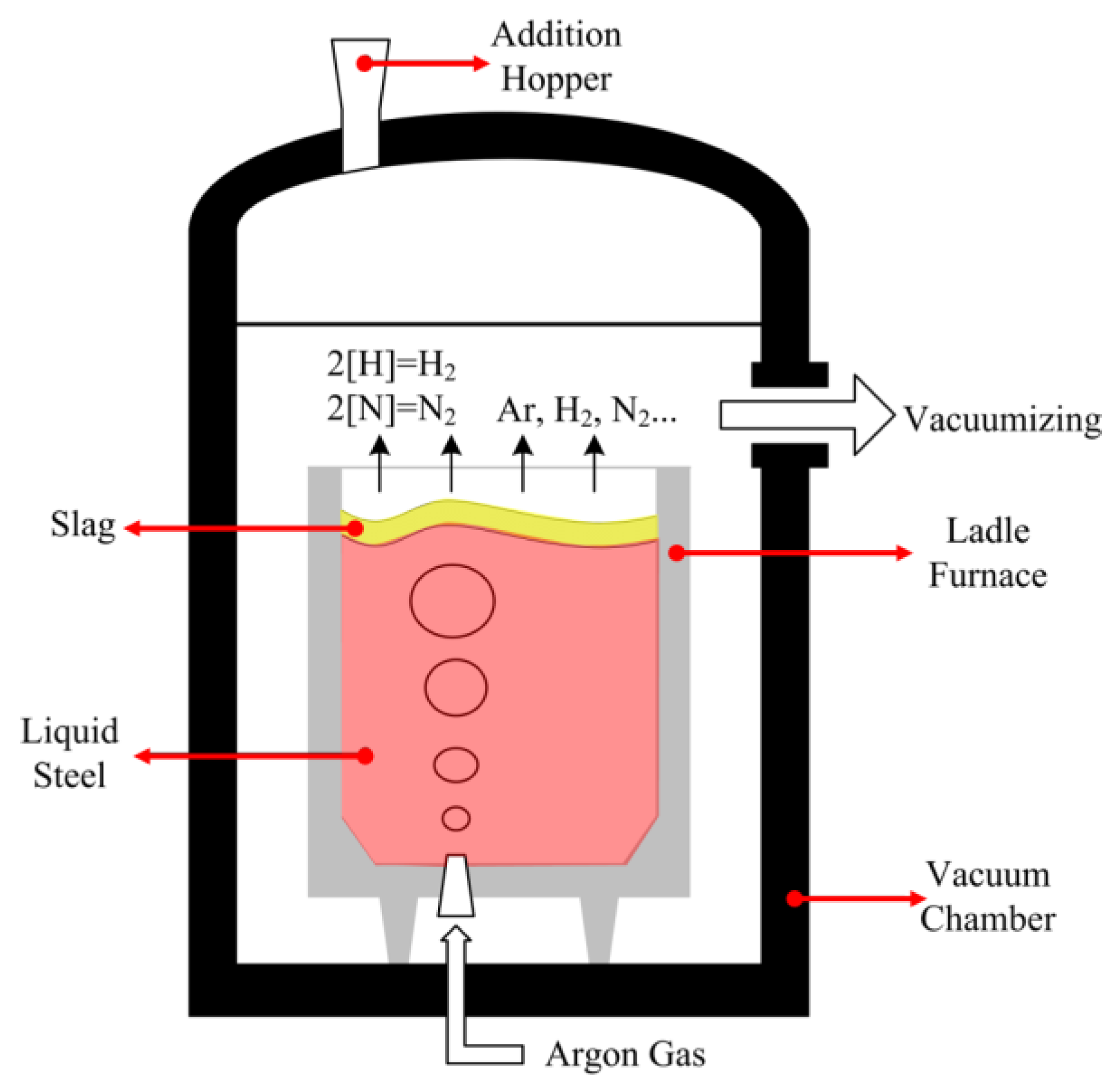
Over the past decades the new materials market has become rapidly competitive. In modern steelmaking, which involves the refining of hot metal in ladles or furnaces and solidifying by continuous casters (CC), clean steels with high quality have been steadily growing because of steel’s mechanical properties have become more and more important for defending steel products against newer competitive materials. In order to produce a satisfactory clean steel with low impurity contents, such as sulfur, phosphorus, non-metallic inclusions, hydrogen, and nitrogen, it is necessary to accurately control the composition and temperature of liquid steel. Steelmakers are urged to improve operating conditions throughout the steelmaking processes to obtain high-purity steel. In practice, the vacuum tank degasser (VTD) is widely used as a secondary steelmaking process to produce steel products with low contents of carbon, hydrogen, and nitrogen. As is schematically illustrated in Figure 1, a refractory lined ladle is installed in a chamber where the ascending gas is pumped out, leading to a very low operating pressure inside the chamber (i.e., 67 Pa). The gas of argon (Ar) is blown into the ladle through the special porous plug(s) or nozzle(s) installed at the bottom of the ladle, and fine bubbles rise from the bottom and disperse into the molten metal. As the argon bubbles rise through the plume, it picks up nitrogen and hydrogen dissolved in the molten metal and leaves the gases maintained at low pressure at the top. In this VTD process, the dissolved impurities in the molten metal were removed partially through two chemical reactions, 2[H] = H2 and 2[N] = N2 (cf. Figure 1).
The aim of VTD system is to obtain liquid steel with the desired composition and temperature. An approach of accelerating the control level of liquid steel in VTD is to forecast the temperature accurately. As the most critical step in the secondary steelmaking process, the VTD has been extensively studied through using various approaches with the goal of better understanding the cause-effect relationships of the vacuum degassing process. Several mathematical models of VTD refining have been developed [1,2,3]. These models were formulated on the basis of differential equations to describe chemical/physical reactions during the production process in the ladle. These mathematical models are local models, dehydrogenation [2] or denitrogenation [3], which depict only part of the property, so it is extremely hard to forecast the temperature of liquid steel using these kinds of white-box models.
An artificial neural network (ANN) is an information process mechanism and can be applied to define the cause-effect relationships between process input parameters and outputs that ‘learn’ directly from historical data. ANNs have been widely applied in the steelmaking process. Gajic et al. [4], for example, have developed the energy consumption model of an electric arc furnace (EAF) based on the feedforward ANNs. Temperature prediction models [5,6] for EAF were established using the neural networks. Rajesh et al. [7] employed feedforward neural networks to predict the intermediate stopping temperature and end blow oxygen in the LD converter steel making process. Wang et al. [8] constructed a molten steel temperature prediction model in a ladle furnace by taking the general regression neural networks as a predictor in their ensemble method. The main feature that makes the neural nets a suitable approach for predicting the temperature drop of liquid steel in VTD is that they are non-linear regression algorithms and can model high dimensional systems. These black-box models offer alternatives to conventional concepts of knowledge representation to solve the prediction problem for an industrial production process system. Volterra polynomial kernel regression (VPKR) is a method to approximate a broad range of input-output maps from sparse and noisy data, which is a central theme in machine learning. The classic Frechét work [9] made contributions to the research topic due to their solid mathematical theory. Moreover, data-driven models based on the VPKR have been found to be useful for nonlinear dynamic systems in industrial applications [10,11]. To address the control problem, the issue could be reduced to solve the nonlinear Volterra integral equations, which have been well studied in heat and power engineering (readers may refer to monograph [12]).
However, in practical manufacturing process applications, black-box prediction is no longer satisfactory. Rule extraction is of vital importance to interpret the understandability of black-box models [13,14,15,16]. The main advantage of rule extraction is that operating decisions can be made for the industry process to promote the controlling level and further improve energy efficiency. Various rule extraction methods have been studied in different application issues. Gao et al. [17], for instance, constructed the rules extraction from a fuzzy-based SVM model for the blast furnace system which used classification and regression trees (CART). Chakraborty et al. [18] proposed a reverse engineering recursive rule extraction (Re-RX) algorithm, which suits for both discrete and continuous attributes in the application issues. Zhou et al. [19] developed a rule extraction mechanism by clustering the process instance data for the manufacturing process design.
In the present work, we propose an integrated method for rule extraction from the VTD black-box model. First is checking the data and eliminating the irrelevant attributes, so not to decrease the model’s expected classification accuracy. Second, fuzzy rules are generated in the form of discrete input attributes (if present) and the target classification. Last but not the least, the rules are refined by generating rules with the continuous attributes (if present). The novelty of the proposed rule extraction approach lies in the generation of rules using the discrete and continuous attributes at different stages. The paper is organized as follows: The extreme learning machine (ELM) network and CART algorithm are briefly presented in the second section. In the third section, the ELM based VTD multiclassifier is established for the end temperature of liquid steel. Section 4 provides the proposed rule extraction method based on the ELM classifier and the rule extraction is shown for the manufacturing process. Finally, conclusions are drawn in the last section.
2. Brief of Related Soft Computing Algorithms
2.1. Extreme Learning Machine
ELM [20] is an efficient learning algorithm for single-hidden layer feedforward neural networks (SLFNs). Based on the least squares method, the ELM algorithm could take place without iterative tuning and reach the globally optimum solution. The output weights between hidden layer and output layer are determined analytically during the learning process [21].
Given a training data set comprising N observations, {xn}, where n = 1, … N, together with corresponding target values, {yn}, the purpose is to predict the value of y for a new value of x. The output function of ELM with L hidden nodes is mathematically represented as:
where βi is the weight vector between the hidden and output layers, ai is the weight vector between the input and hidden layers, bi is the bias of the ith hidden node, G(ai, bi, xj) is the output function of the ith hidden node, and ŷj is the output predictive value.
According to the ELM theory, the main idea of ELM is to predict the training set with zero error, i.e., , which implies that there exists (ai, bi) and βi satisfies the following:
Equation (2) can be rewritten as
where
As defined in ELM, H is the output matrix of hidden layer. The aim is to calculate the output weights β in minimizing the norm of β, as well as the training errors. The mathematical issue can be represented as follows:
where C is a user-specified parameter and ξi is the training error.
Based on the Karush-Kuhn-Tucker (KKT) theorem, to train the ELM is equal to solving the following optimization problem:
where αi is the Lagrange multiplier.
Two different solutions to the dual optimization problem can be achieved with different sizes of the training data set.
1. The training set is not huge:
The corresponding output function of ELM is
2. The training set is huge:
The corresponding output function of ELM is
These two solutions have different computational costs in the implementation of ELM. In the application of the small training data set (N<<L), Equation (9) can increase the learning speed. However, if the size of training data is huge (N>>L), one may prefer to use the Equation (11) instead.
For multiclass cases, the predicted class label of a given test sample is the index number of the highest output node. Let fi(x) denote the output function of the ith output function of the ith output node, i.e., f(x) = [f1(x), …, fm(x)]T, then the predicted class label of input vector x is
2.2. Classification and Regression Trees
The CART decision tree proposed by Breiman et al. [22] is a binary tree structure to construct classification or regression models from data. In this study, we want to search the IF-THEN rules using the classification case of CART. In the CART algorithm, the maximal binary tree is constructed by partitioning the training data space recursively. Then, the maximal binary tree is pruned based on the Occam’s razor principle. To grow the binary tree, the Gini index is used to find the root node with the minimized value of the feature. The procedure of the CART algorithm is presented as follows.
Step 1: Given a training data set, S, comprising N observations, {xi}, where i = 1, 2, …, N, together with corresponding target m classes, {yik}, where k = 1, 2, …, m, set pj (j = 1, 2, …, m) as the probabilities of each class and satisfy . The Gini index Gi(S) is defined as
Step 2: Calculate the Gini indexes of all partition nodes as
where S1 and S2 are the subsets of S divided by a certain condition C and N1 and N2 are the numbers of the patterns in S1 and S2, respectively. For the continuous input variable, the average of two adjacent values is thought as a candidate partition node. Thus, there are total (N − 1) × n possible partition nodes in the data set with n continuous variables.
Step 3: Find the optimal partition node from all the possible partition nodes with the lowest Gini index. The corresponding variable is the root node and the threshold is the branch condition under the root node. Two subsets are produced after the root node. The same procedure is applied recursively to the two subsets to generate the maximal binary tree.
Step 4: Prune the maximal binary tree by cutting off some branches without increasing the cost-complexity, which produces a sequence of subtrees consisting of the root node.
Step 5: Select the optimal subtree from the candidate subtrees using the cross-validation method.
3. ELM-Based Classification for VTD
3.1. Production Data
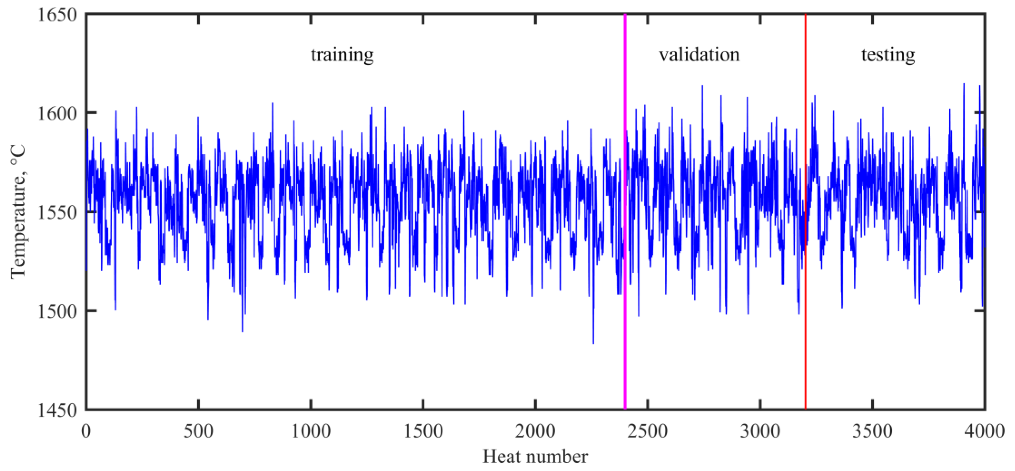
In the present work, the experimental data were collected from a No.2 steelmaking workshop in Baosteel. A total of 4000 observations during normal operations in VTD were collected for modelling purposes. Each observation contained discrete attributes (ladle material, refractory life, and heat status) and 16 continuous process parameters. Of the data, 2400 observations (60%) were used for training, 800 observations (20%) were used for validating, and the remaining 800 observations (20%) were used for testing. Figure 2 shows the evolution of the end temperature in the VTD.
Table 1 tabulates the attribute information from the VTD system, in which the discrete attributes are converted into binary inputs with the use of the one-hot encoding method. The continuous attributes are labeled as C1, C2, …, C16 and the discrete attributes are labeled as D1, D2, …, D9.
3.2. Three-Class of the End Temperature
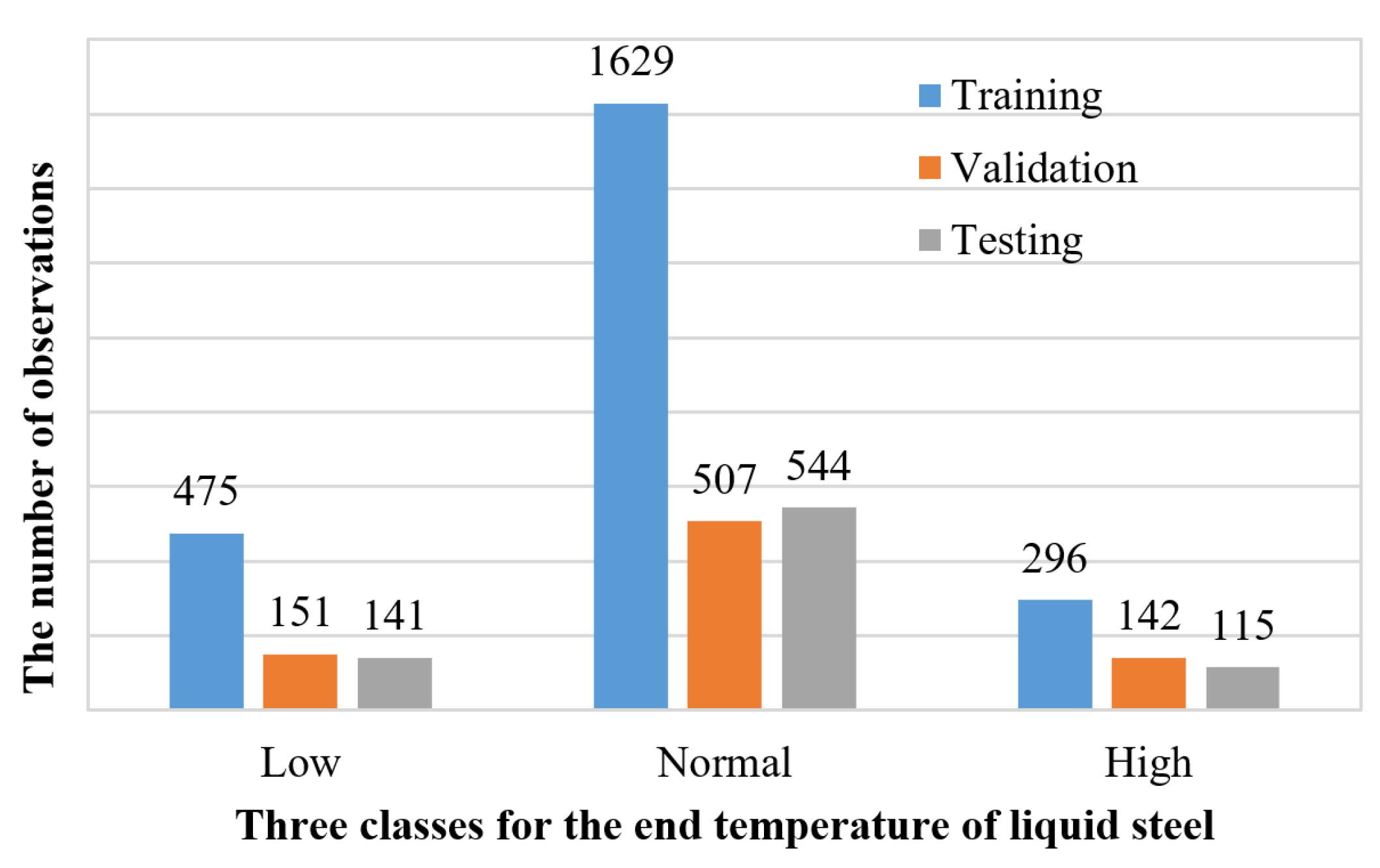
To construct the three-class classifier for the end temperature of liquid steel in the VTD system, the controlled bound of the temperature needs to be determined. In the statistics, a large amount of the individual samples were located within the range [μ − σ, μ + σ], where μ stands for the expected value and σ stands for the standard deviation. To capture the main property of the end temperature in VTD, we formed the normal end temperature bound as [μ − σ, μ + σ], i.e., [1535.6 °C, 1574.3 °C] for the VTD. The experimental data are classified to three classes, as follows: Low end temperature (<1535.6 °C) labeled as class 1, normal end temperature ([1535.6 °C, 1574.3 °C]) labeled as class 2, and high-end temperature (>1574.3 °C) labeled as class 3. Figure 3 shows the sample distributions on the three classes. Class 1 and class 3 represent 19.175% (767 observations) and 13.825% (553 observations) of the data set, respectively, and the remaining 67% (2680 observations) are classified as class 2.
3.3. ELM-Based Three-Class Classification of the End Temperature
To design a three-class classifier for the end temperature of VTD, a three-class ELM classifier was established in this study. For the ELM network, the sigmoid function g(x) = 1/(1 + exp(−x)) was selected as the activation function. The cost parameter C was selected from {2−24, 2−23, …, 224, 225} and the number of hidden nodes L was selected from {10, 20, …, 1000}. In our simulations, all the input attributes were normalized into [0, 1]. The optimal parameter combination (C, L) was determined by the prediction accuracy on validation set. The parameter combination (C, L) was selected with the highest validation set accuracy (VSA). Here, the VSA is defined as the ratio of the number of the correct classifications to the validation set size. With the optimal parameter combination, the ELM-based three-class classifier was used to perform the classification task on the testing data set and the results are tabulated in Table 2. As shown in Table 2, we can get the following information: (1) The training accuracy (TRA) is satisfactory, reaching 80.33% for the VTD; (2) the testing accuracy (TEA) is 71.88% and is encouraging for the end temperature prediction in the VTD system; (3) the predictions for the end temperature in the normal bound are credible for the correct rate, attaining 472/544 = 86.76%, while the predictions for outside the normal bound are unreliable; and (4) overfitting exists due to the large difference between the TRA and the VSA; therefore, methods should be developed to reduce the overfitting. From these results, the three-class classification method for the end temperature is effective in the VTD system.
To reduce the overfitting of the model, feature selection is conducted on the VTD input sets to establish the robust classifier. In this study, a feature pruning method was proposed to remove the irrelevant features from the original attributes set if the classification accuracy increases after pruning. The method first validates the accuracy, A0, of the initial accuracy, Fj, with the input feature set. It than calculates accuracy Anew by removing each feature from Fj. The approach removes the feature ni from Fj if Anew ≥ A0. The mechanism for feature pruning is given below.
The VSA in Table 2, with the 25 inputs, was used as the initial accuracy. If the removal of a feature can make the VSA higher than the previous one, the feature is removed. Finally, 19 features were selected out and are presented in Table 1. Furthermore, to make a comparison, the results with these new features are tabulated in Table 2. It is clear that the feature selection helps to improve the performance of the ELM classifier. The overfitting is reduced and there is a little increase of TEA, which implies that the classification model can be promoted by feature pruning. In addition, the predictions for the end temperature in the normal bound kept reliability for the correct rate, attaining 478/544 = 87.87%.
4. Rules Extraction for VTD
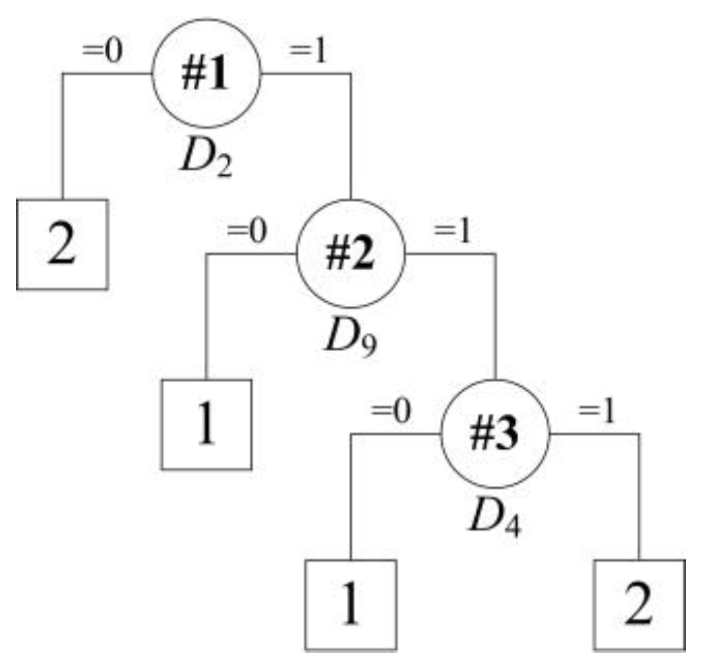
The ELM-based three-class classifier can effectively classify the end temperature into low, normal, and high regions. However, the mechanism in this black-box model is still unknown to the operators for the decision-making propose in a VTD system. To this end, rule extraction is further important for the practical manufacturing process. The correct classified samples by the ELM model after feature selection in the training set were used as the current training set. Thus, the training samples come to 1909 (79.54% of the original training set) in the current training set, while the current testing set was still the original one. As there are continuous and discrete attributes in classification of the end temperature of the VTD system, different approaches should be made in this setting. For the binary discrete attributes, a binary tree is generated using the CART algorithm, as shown in Figure 4.
The following set of rules is obtained after embodying the binary tree rules:
- Rule R1: IF D2 = 0, THEN the predict class = 2;
- Rule R2: IF D2 = 1 and D9 = 0, THEN the predict class = 1;
- Rule R3: IF D2 = 1 and D9 = 1 and D4 = 0, THEN the predict class = 1;
- Rule R4: IF D2 = 1 and D9 = 1 and D4 = 1, THEN the predict class = 2.
The classification results on the current training dataset by application of the CART algorithm using only the binary attributes are summarized in Table 3. The support denotes the percentage of samples that are covered by the rule. The error is the misclassified percentage in a rule.
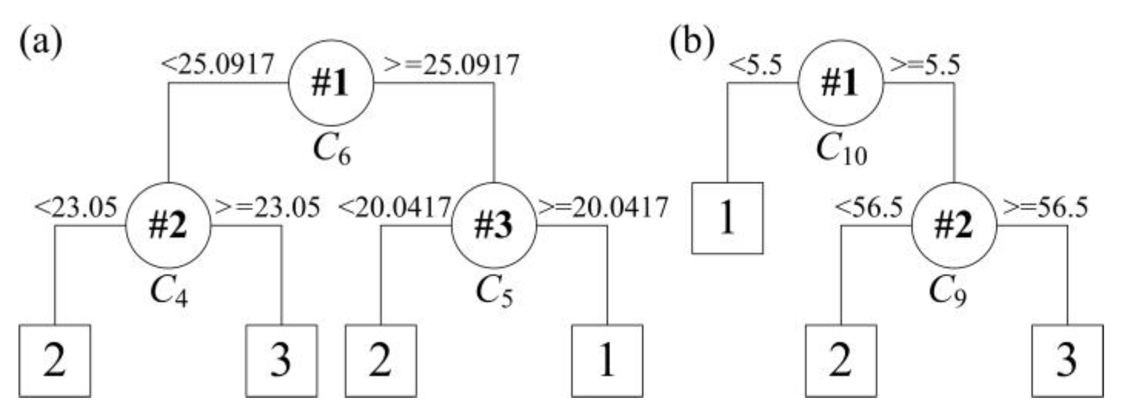
The support threshold δ1 and error threshold δ2 were set to 0.05. From Table 3, it can be seen that the rule R1 and R2 should be refined to improve the classification accuracy. So, rules are generated for the unclassified samples by using the continuous attributes. The binary classification tree can be created by applying the CART algorithm using the continuous attributes. Four rules are obtained for classification of the unclassified samples in rule R1. Similarly for rule R2, three rules are generated for classification of the unclassified samples. The two sub binary trees are depicted in Figure 5.
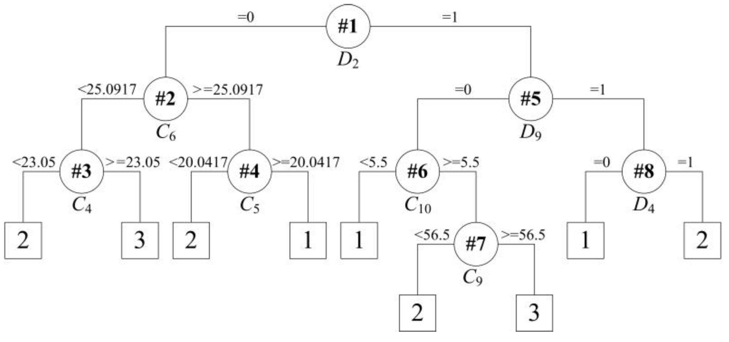
The ultimate binary tree is obtained after embedding the two sub binary trees with continuous attributes into the first binary tree with discrete attributes, which is depicted in Figure 6. The ultimate rules are exhibited as follows:
Rule R1: IF D2= 0, follows:
- Rule R1a: IF C6 < 25.0917 and C4 < 23.05, THEN predict class = 2;
- Rule R1b: IF C6 < 25.0917 and C4 ≥ 23.05, THEN predict class = 3;
- Rule R1c: IF C6 ≥ 25.0917 and C5 < 20.0417, THEN predict class = 2;
- Rule R1d: IF C6 ≥ 25.0917 and C5 ≥ 20.0417, THEN predict class = 1;
Rule R2: IF D2 = 1 and D9 = 0, follows:
- Rule R2a: IF C10 < 5.5, THEN predict class = 1;
- Rule R2b: IF C10 ≥ 5.5 and C9 < 56.5, THEN predict class = 2;
- Rule R2c: IF C10 ≥ 5.5 and C9 ≥ 56.5, THEN predict class = 3;
Rule R3: IF D2 = 1 and D9 = 1 and D4 = 0, THEN the predict class = 1;
Rule R4: IF D2 = 1 and D9 = 1 and D4 = 1, THEN the predict class = 2.
From the above rules, only eight attributes are needed (three discrete features and five continuous features) to judge the end temperature as being low, normal, or high. The discrete attributes describe the ladle conditions and are of vital importance to the end temperature of liquid steel in a VTD. The property of heat transfer through the ladle is different due to the different ladle materials. The refractory life of the ladle represents the thickness of the interior thermal insulation material, which is the main heat absorbing media during the transportation of the liquid steel. The heat status indicates the temperature of the interior thermal insulation material. In the practical manufacturing process, the tap temperature is adjusted according to the heat status of the ladle furnace. This is the temperature correction stage in the VTD system. The five continuous attributes are soft stirring time C6, arrive high vacuum time C4, keep vacuum time C5, wire feed consumption type 2 C10, and wire feed consumption type 1 C9. These features are the key operating parameters in the VTD system and control the vacuum degassing process. All these results reveal that the rules extracted from the ELM-based classification model are reasonable and convenient for use in decision-making in the VTD system.
From the previous discussion, the rule extraction methodology from the ELM-based classification for the VTD system can be summarized as follows (Algorithm 1):
| Algorithm 1: Rule extraction from ELM classification |
| Input: Training data set S = {(xi, ti)}, i = 1, 2, …, N, xi∈Rn, ti∈R, with discrete attributes D and continuous attributes C. |
| Output: A set of classification rules. |
| 1: Calculate the expected value μ and the standard deviation σ of the target series |
| 2: for i = 1 to N do |
| 3: if ti < μ − σ, then, yi = 1. |
| 4: if μ − σ ≤ ti ≤ μ + σ, then, yi = 2. |
| 5: if ti > μ + σ, then, yi = 3. |
| 6: end for |
| 7: Switch the discrete attributes D into binary inputs with the use of the one-hot encoding method. |
| 8: Normalize the continuous attributes C into [0, 1]. |
| 9: Train an ELM using the data set S with all its attributes D and C. |
| 10: Prune the ELM classifier to obtain the new D’ and C’. Let S’ be the set of samples that are correctly classified by the pruned ELM network. |
| 11: If D’ = ϕ, then generate a binary tree using the continuous attributes C’ and stop. |
| 12: Otherwise, generate binary tree rules R using only the D’ with the data set S’. |
| 13: for each rule Ri do |
| 14: if support(Ri) > δ1 and error(Ri) > δ2, then |
| 15: Generate binary tree rules using continuous attributes C’ with the data set Si’ that satisfy the condition of rule Ri. |
| 16: end for |
Further apply the proposed method to predict the end temperature of VTD; the extracted rules are verified by the testing data set. The results are evaluated based on the values of accuracy (the ratio of the correct predictions on the testing data set) and fidelity (the ability of the extracted rules that mimic the black-box model).
where TP, TN, FP, and FN represent the abbreviation of true positives, true negatives, false positives, and false negatives, respectively.
Table 4 shows the classification results using the extracted rules. The accuracy reached 75%, higher than the ELM classifier, which is 72.75% on the testing data set after feature selection. In addition, a large amount of the corrected predictions by the ELM classifiers can also be correctly classified by the extracted rules. That is to say, the extracted rules can accurately mimic the black-box ELM model. Moreover, the extracted rules only need eight features, far less than the 19 features in the ELM classification model. Another notable point is that the extracted rules are explicit information items for classifying the end temperature into low, normal, or high range. Therefore, the extracted rules can be directly used in the VTD system for decision-making with desirable accuracy.
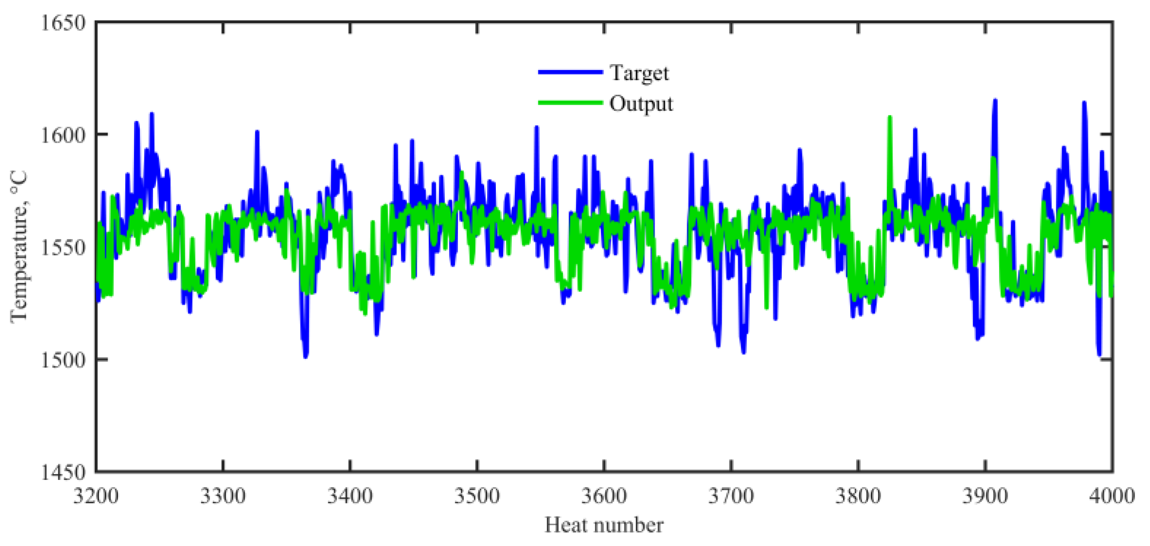
To explain the feasibility and effectiveness of our proposed method, a comparison with the ELM regression model was conducted. It should be noted that the ELM regression model can only predict the numerical values of the end temperature and cannot give the direct three-class classification results. Therefore, the numerical predictions were converted into the classification result according to the temperature divisions. As discussed above, there are eight features reserved in the hybrid rule extraction model. The five continuous attributes are arrive high vacuum time C4, keep vacuum time C5, soft stirring time C6, wire feed consumption type 1 C9, and wire feed consumption type 2 C10. The 3 discrete attributes are ladle material type 2 D2, refractory life type 1 D4 and heat status type 3 D9. Thus, a fair comparison can be conducted if these attributes are fed into the ELM regression model. Figure 7 depicts the prediction results of the end temperature on the testing set. Further switching these numerical prediction values into the three-class classification results can obtain a TEA of 74.12%. From the viewpoint of TEAs, the ELM regression model is weaker than the proposed integrated classification model with the same input attributes. In addition, the ELM regression model trained the non-liner function in the black-box and the rules generated are unclear in this black-box model.
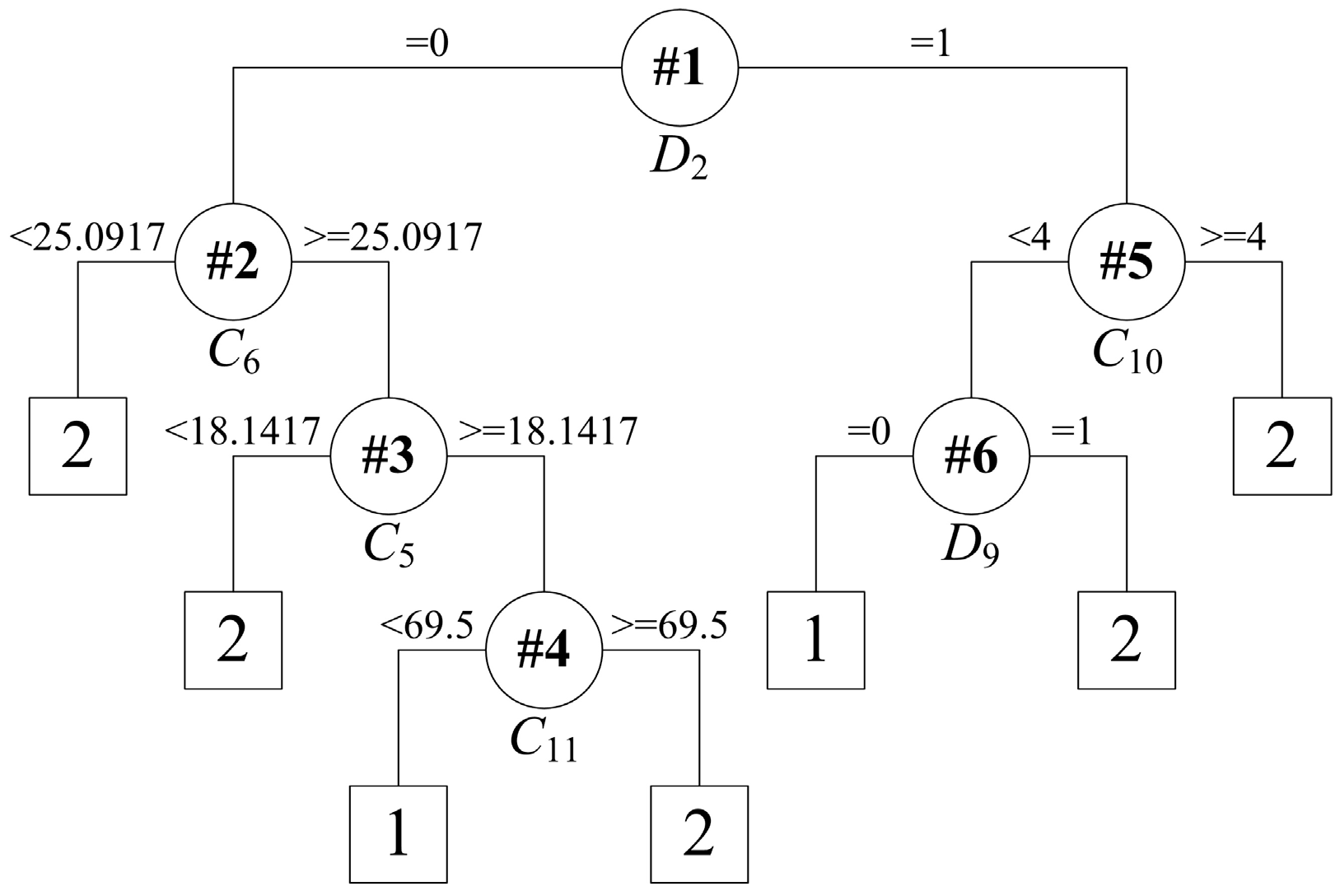
As a rule extraction approach, the CART algorithm can work independently of the trained ELM model. Figure 8 depicts the binary tree built by the CART algorithm using the original training data set with all 25 of the attributes. The testing results are shown in Table 4. Although fewer features are used in the CART model, the extracted rules, as shown in Figure 8, were a little one-sided, with no high-end temperature rule. At this point, they cannot cover all cases reflecting the end temperature range. Thus, the rules extracted directly from the original training data set with all the features have difficulty in capturing the characteristics of the VTD system. This undesirable performance indicates that the combination of the ELM and the CART algorithm is an essential method to extract rules for the VTD system.
From the viewpoint of addressing the end temperature control problem in the VTD system, the proposed strategy provides a novel modeling thought that makes the black-box model transparent to the operators. It integrates the advantages of the ELM classification model and the CART algorithm. The novelty of the current work is to develop a rule extraction method for controlling the end temperature within a certain range. Since process control would be the ultimate purpose and the VTD system control often means controlling the temperature and composition of liquid steel within desirable bounds, the extracted rules can play a role in making transparent decisions versus the black-box model. Compared with the direct numerical prediction methods, such as ELM, the current work can mimic the black-box model with enhanced transparency. Another important contribution made in this work is using CART to improve ELM classification for rule extraction. The direct CART applications [23,24,25] have been widely studied for different technological issues. These developments are probably due to that the CART algorithm is essentially a kind of white-box modelling approach. The CART method can be used to extract rules from data with mixed attributes. However, the one-sided rules obtained using the original training data set in our study cannot be applied to the practical manufacturing process. Therefore, we propose a hybrid method that uses the CART to extract rules from the trained ELM black-box model, through which all-sided rules have been obtained and the advantage of ELM black-box model for the VTD system can be fully mined. Of course, the proposed methodology can be applied to address other industry manufacturing process control issues. Additionally, the classification method and rule extraction algorithm is not limited to ELM and CART algorithms. Other classification algorithms, like ANNs [26] and SVMs [27], and other rule extraction approaches, like C4.5 [28] and the Re-RX algorithm [29], can work as well within the proposed hybrid strategy. For further research, it could be interesting to extend the proposed framework for dealing with other manufacturing problems by testing other combinations, such as ANNs and C4.5, SVMs and Re-RX algorithm, etc.
The main motivation to pursue the current research is that the operation of VTD systems is still a serious problem in practice. The all-sided rules have been extracted from the production data by combining the ELM and CART algorithms. The most important reason is that the features are pruned according to the prediction results of ELM model and the patterns are well confirmed to capture the dynamic properties. Another more important reason is that the CART algorithm is essentially a kind of white-box modeling method to extract process control strategies. Hence, the proposed method presents a novel strategy to obtain a solution for the VTD control issue.
5. Conclusions
In this paper, a method of rules extraction from the trained ELM classification model for the decision-making purposes has been presented. Firstly, a three-class classification problem of the end temperature in the VTD system has been constructed according to the practical control mechanism. Secondly, an ELM multiclassifier has been developed to instruct the end temperature in low, normal, or high ranges. Finally, based on the pruned and correctly classified training data set, rules are extracted with discrete and continuous features utilizing the CART algorithm. The proposed method has the ability to successfully classify the end temperature, which demonstrates the potential for reliable prediction of the end temperature in a VTD system. The extracted rules can act as a potential tool for predicting the end temperature in advance, which will be helpful in precisely controlling the process of VTD systems.
In the future, the proposed model will be further developed. More data sources from different industrial fields and more factors will be applied to this model in order to verify the feasibility and further optimal model parameters to obtain higher predicting accuracies. If the above-mentioned method is proved to be practical, other similar refining processes will be considered to develop a new model based on an integrated methodology for rule extraction from an ELM-Based multi-classifier, and this model is expected to be used as a what-if tool to provide a practical guide in the future.
Author Contributions
Conceptualization, S.W., H.L. and Z.Z.; Funding acquisition, H.L.and Z.Z.; Investigation, S.W.; Methodology, Y.Z. Project administration, Y.Z.; Resources, Y.Z.; Supervision, Y.Z.; Validation, S.W. and H.L.; Writing—original draft, S.W.; Writing—review & editing, Z.Z.
Funding
This research was funded by National Key Research and Development Program, grant number 2017YFB0603800, 2017YFB0603802 and China Scholarship Council, grant number 201706085021.
Conflicts of Interest
The authors declare no conflict of interest. The funders had no role in the design of the study; in the collection, analyses, or interpretation of data; in the writing of the manuscript, or in the decision to publish the results.
References
- Thapliyal, V.; Lekakh, S.N.; Peaslee, K.D.; Robertson, D.G.C. Novel modeling concept for vacuum tank degassing. In Proceedings of the Association for Iron & Steel Technology Conference, Atlanta, GA, USA, 7–10 May 2012; pp. 1143–1150. [Google Scholar]
- Yu, S.; Louhenkilpi, S. Numerical simulation of dehydrogenation of liquid steel in the vacuum tank degasser. Metall. Mater. Trans. B-Process Metall. Mater. Process. Sci. 2013, 44, 459–468. [Google Scholar] [CrossRef]
- Yu, S.; Miettinen, J.; Shao, L.; Louhenkilpi, S. Mathematical modeling of nitrogen removal from the vacuum tank degasser. Steel Res. Int. 2015, 86, 466–477. [Google Scholar] [CrossRef]
- Gajic, D.; Savic-Gajic, I.; Savic, I.; Georgieva, O.; di Gennaro, S. Modelling of electrical energy consumption in an electric arc furnace using artificial neural networks. Energy 2016, 108, 132–139. [Google Scholar] [CrossRef]
- Kordos, M.; Blachnik, M.; Wieczorek, T. Temperature prediction in electric arc furnace with neural network tree. In Proceedings of the International Conference on Artificial Neural Networks, Espoo, Finland, 11–14 June 2011; pp. 71–78. [Google Scholar]
- Fernandez, J.M.M.; Cabal, V.A.; Montequin, V.R.; Balsera, J.V. Online estimation of electric arc furnace tap temperature by using fuzzy neural networks. Eng. Appl. Artif. Intell. 2008, 21, 1001–1012. [Google Scholar] [CrossRef]
- Rajesh, N.; Khare, M.R.; Pabi, S.K. Feed forward neural network for prediction of end blow oxygen in LD converter steel making. Mater. Res. Ibero-Am. J. Mater. 2010, 13, 15–19. [Google Scholar] [CrossRef] [Green Version]
- Wang, X.J.; You, M.S.; Mao, Z.Z.; Yuan, P. Tree-structure ensemble general regression neural networks applied to predict the molten steel temperature in ladle furnace. Adv. Eng. Inform. 2016, 30, 368–375. [Google Scholar] [CrossRef]
- Frechét, M. Sur les fonctionnelles continues. Annales Scientifiques de l’École Normale Supérieure 1910, 27, 193–216. [Google Scholar] [CrossRef] [Green Version]
- Doyle, F.J.; Pearson, R.K.; Ogunnaike, B.A. Identification and Control Using Volterra Models; Springer: London, UK, 2002; pp. 79–103. [Google Scholar]
- Gao, C.H.; Jian, L.; Liu, X.Y.; Chen, J.M.; Sun, Y.X. Data-Driven Modeling Based on Volterra Series for Multidimensional Blast Furnace System. IEEE Trans. Neural Netw. 2011, 22, 2272–2283. [Google Scholar] [PubMed]
- Sidorov, D. Integral Dynamical Models: Singularities, Signals & Control. World Scientific Series on Nonlinear Science Series A; Chua, L.O., Ed.; World Scientific Publishing: Singapore, 2015. [Google Scholar]
- Duch, W.; Setiono, R.; Zurada, J.M. Computational intelligence methods for rule-based data understanding. Proc. IEEE 2004, 92, 771–805. [Google Scholar] [CrossRef] [Green Version]
- Barakat, N.; Bradley, A.P. Rule extraction from support vector machines a review. Neurocomputing 2010, 74, 178–190. [Google Scholar] [CrossRef]
- Chen, Y.C.; Pal, N.R.; Chung, I.F. An integrated mechanism for feature selection and fuzzy rule extraction for classification. IEEE Trans. Fuzzy Syst. 2012, 20, 683–698. [Google Scholar] [CrossRef]
- De Falco, I. Differential evolution for automatic rule extraction from medical databases. Appl. Soft Comput. 2013, 13, 1265–1283. [Google Scholar] [CrossRef]
- Gao, C.H.; Ge, Q.H.; Jian, L. Rule extraction from fuzzy-based blast furnace SVM multiclassifier for decision-making. IEEE Trans. Fuzzy Syst. 2014, 22, 586–596. [Google Scholar] [CrossRef]
- Chakraborty, M.; Biswas, S.K.; Purkayastha, B. Recursive rule extraction from NN using reverse engineering technique. New Gener. Comput. 2018, 36, 119–142. [Google Scholar] [CrossRef]
- Zhou, J.T.; Li, X.Q.; Wang, M.W.; Niu, R.; Xu, Q. Thinking process rules extraction for manufacturing process design. Adv. Manuf. 2017, 5, 321–334. [Google Scholar] [CrossRef] [Green Version]
- Huang, G.B.; Zhou, H.M.; Ding, X.J.; Zhang, R. Extreme learning machine for regression and multiclass classification. IEEE Trans. Syst. Man Cybern. Part B-Cybern. 2012, 42, 513–529. [Google Scholar] [CrossRef] [PubMed]
- Liu, X.Y.; Gao, C.H.; Li, P. A comparative analysis of support vector machines and extreme learning machines. Neural Netw. 2012, 33, 58–66. [Google Scholar] [CrossRef]
- Breiman, L.; Friedman, J.H.; Olshen, R.A.; Stone, C.J. Classification and Regression Trees; Chapman & Hall: London, UK, 1984. [Google Scholar]
- Zimmerman, R.K.; Balasubramani, G.K.; Nowalk, M.P.; Eng, H.; Urbanski, L.; Jackson, M.L.; Jackson, L.A.; McLean, H.Q.; Belongia, E.A.; Monto, A.S.; et al. Classification and regression tree (cart) analysis to predict influenza in primary care patients. BMC Infect. Dis. 2016, 16, 1–11. [Google Scholar] [CrossRef]
- Salimi, A.; Faradonbeh, R.S.; Monjezi, M.; Moormann, C. TBM performance estimation using a classification and regression tree (cart) technique. Bull. Eng. Geol. Environ. 2018, 77, 429–440. [Google Scholar] [CrossRef]
- Cheng, R.J.; Yu, W.; Song, Y.D.; Chen, D.W.; Ma, X.P.; Cheng, Y. Intelligent safe driving methods based on hybrid automata and ensemble cart algorithms for multihigh-speed trains. IEEE Trans. Cybern. 2019, 49, 3816–3826. [Google Scholar] [CrossRef]
- Ng, S.C.; Cheung, C.C.; Leung, S.H. Magnified gradient function with deterministic weight modification in adaptive learning. IEEE Trans. Neural Netw. 2004, 15, 1411–1423. [Google Scholar] [CrossRef] [PubMed]
- Cortes, C.; Vapnik, V. Support-vector networks. Mach. Learn. 1995, 20, 273–297. [Google Scholar] [CrossRef]
- Quinlan, J.R. C4.5: Programs for Machine Learning; Morgan Kaufmann Publishers: Los Altos, CA, USA, 1993. [Google Scholar]
- Setiono, R.; Baesens, B.; Mues, C. Recursive neural network rule extraction for data with mixed attributes. IEEE Trans. Neural Netw. 2008, 19, 299–307. [Google Scholar] [CrossRef] [PubMed]
Figure 1.
Schematic representation of a VTD.

Figure 2.
Evolution of the end temperature in the VTD.

Figure 3.
Distribution of the temperature points in terms of low, normal, and high. The numbers on the top of each column denote the values of the ordinates, for example 475 indicates that there are 475 points that fall into the low temperature range for the training data set. The meaning of the other numbers is analogous.

Figure 4.
Tree structure for rule extraction on the dataset with correct classifications using only discrete attributes.
Figure 4.
Tree structure for rule extraction on the dataset with correct classifications using only discrete attributes.

Figure 5.
Tree structure for rule extraction on the dataset of rule R1 (a) and R2 (b).

Figure 6.
Tree structure for rule extraction on the dataset with correct classifications.

Figure 7.
Numerical predictions of the end temperature through the ELM regression model, based on the testing set.
Figure 7.
Numerical predictions of the end temperature through the ELM regression model, based on the testing set.

Figure 8.
Tree structure for rule extraction on the original training set.


Table 1.
List of candidate input attributes from VTD.
| Attribute Name | Unit | Input Attributes |
|---|---|---|
| Liquid steel weight | t | |
| Tap temperature | °C | |
| Tap to vacuum time | min | |
| Arrive high vacuum time | min | |
| Keep vacuum time | min | |
| Soft stirring time | min | |
| Refining time | min | |
| Argon consumption | m3 | |
| Wire feed consumption | kg | , , , C12 |
| Alloy consumption | kg | , C14, , |
| Ladle material | - | D1, , |
| Refractory life | - | , D5, |
| Heat status | - | , D8, |
1 Attributes with wave line are the input attributes after feature selection.
Table 2.
Evaluation of the predictive performance of the proposed model.
| Inputs | Distribution | End Temperature (°C) | TRA | VSA | TEA | ||
|---|---|---|---|---|---|---|---|
| Low | Normal | High | (%) | (%) | (%) | ||
| 25 | true | 141 | 544 | 115 | 80.33 | 63.75 | 71.88 |
| prediction | 154 | 622 | 24 | ||||
| correct | 95 | 472 | 8 | ||||
| 19 | prediction | 152 | 627 | 21 | 79.54 | 66.13 | 72.75 |
| correct | 97 | 478 | 7 | ||||
Table 3.
Support level and error rate of the rules generated using CART with only discrete attributes.
Table 3.
Support level and error rate of the rules generated using CART with only discrete attributes.
| Rules | #Samples | Correct | Wrong | Support | Error |
|---|---|---|---|---|---|
| Classification | Classification | (%) | (%) | ||
| R1 | 1510 | 1412 | 98 | 79.10 | 6.49 |
| R2 | 322 | 266 | 56 | 16.87 | 17.39 |
| R3 | 8 | 6 | 2 | 0.42 | 25.00 |
| R4 | 69 | 63 | 6 | 3.61 | 8.70 |
| All rules | 1909 | 1747 | 162 | 100 | 8.49 |
Table 4.
Results of rule extraction for VTD system.
| Method | Attributes | Rules | Accuracy (%) | Fidelity (%) |
|---|---|---|---|---|
| Proposed | 8 | 9 | 75 | 89.75 |
| CART | 6 | 7 | 74 | 88.50 |
© 2019 by the authors. Licensee MDPI, Basel, Switzerland. This article is an open access article distributed under the terms and conditions of the Creative Commons Attribution (CC BY) license (http://creativecommons.org/licenses/by/4.0/).
Share and Cite
MDPI and ACS Style
Wang, S.; Li, H.; Zhang, Y.; Zou, Z. An Integrated Methodology for Rule Extraction from ELM-Based Vacuum Tank Degasser Multiclassifier for Decision-Making. Energies 2019, 12, 3535. https://doi.org/10.3390/en12183535
AMA Style
Wang S, Li H, Zhang Y, Zou Z. An Integrated Methodology for Rule Extraction from ELM-Based Vacuum Tank Degasser Multiclassifier for Decision-Making. Energies. 2019; 12(18):3535. https://doi.org/10.3390/en12183535
Chicago/Turabian StyleWang, Senhui, Haifeng Li, Yongjie Zhang, and Zongshu Zou. 2019. "An Integrated Methodology for Rule Extraction from ELM-Based Vacuum Tank Degasser Multiclassifier for Decision-Making" Energies 12, no. 18: 3535. https://doi.org/10.3390/en12183535
Note that from the first issue of 2016, this journal uses article numbers instead of page numbers. See further details here.