Prognostics Comparison of Lithium-Ion Battery Based on the Shallow and Deep Neural Networks Model

School of Automation Engineering, University of Electronic Science and Technology of China (UESTC), Chengdu 611731, China
*
Author to whom correspondence should be addressed.
Energies 2019, 12(17), 3271; https://doi.org/10.3390/en12173271
Submission received: 16 July 2019
/
Revised: 20 August 2019
/
Accepted: 20 August 2019
/
Published: 25 August 2019
Abstract
:Prognostics of the remaining useful life (RUL) of lithium-ion batteries is a crucial role in the battery management systems (BMS). An artificial neural network (ANN) does not require much knowledge from the lithium-ion battery systems, thus it is a prospective data-driven prognostic method of lithium-ion batteries. Though the ANN has been applied in prognostics of lithium-ion batteries in some references, no one has compared the prognostics of the lithium-ion batteries based on different ANN. The ANN generally can be classified to two categories: the shallow ANN, such as the back propagation (BP) ANN and the nonlinear autoregressive (NAR) ANN, and the deep ANN, such as the long short-term memory (LSTM) NN. An improved LSTM NN is proposed in order to achieve higher prediction accuracy and make the construction of the model simpler. According to the lithium-ion data from the NASA Ames, the prognostics comparison of lithium-ion battery based on the BP ANN, the NAR ANN, and the LSTM ANN was studied in detail. The experimental results show: (1) The improved LSTM ANN has the best prognostic accuracy and is more suitable for the prediction of the RUL of lithium-ion batteries compared to the BP ANN and the NAR ANN; (2) the NAR ANN has better prognostic accuracy compared to the BP ANN.
1. Introduction
Lithium-ion batteries have been widely used from portable electronics to battery-driven hybrid vehicles owing to their higher energy density, higher output voltage, lower self-discharge, longer lifetime, higher reliability and other advantages compared to other types of batteries available in the market [1,2,3]. The lithium-ion battery failure consequence have different levels of severity: from performance degradation to catastrophic failure [4]. The lithium-ion battery failure caused several Boeing 787 to be caught fire and caused all airliners to be grounded indefinitely in 2013 [5]. Therefore, It is imperative and highly desired to detect the performance degradation and to predict the remaining useful life (RUL) of lithium-ion batteries. Prognostics and health management (PHM) are the technologies to evaluate the reliability of a system in its actual life cycle conditions to determine the RUL [6,7]. One of the major work of prognostics is to predict RUL [1]. In this paper, we consider the battery will fail when the battery’s capacity drops to 70% of its initial capacity, because both the battery’s capacity and power will drop much faster after this point, and the battery is unreliable and should be replaced [8,9].
Existing methods for lithium-ion batteries’ RUL prediction roughly can be classified into two main categories: the physics-of-failure (PoF)-based method and the data-driven method [1,2]. The PoF-based prognostic methods depend on the battery physical characteristics, i.e., a battery’s material property, its failure mechanism and life cycle loading conditions, and tend to be computationally complex [10]. Thus, the data-driven prognostic approach have widely been used because it does not require the extensive knowledge mentioned before. Among data-driven prognostic approaches, the particle filter (PF) and relevance vector machine (RVM) are two popular lithium-ion batteries’ RUL prognostic approach [1]. PF is a sequential Monte Carlo method, which estimates the state probability distribution function (PDF) from a set of “particles” and their associated weights [1]. Long [2] proposed prognostic approach for lithium-ion batteries RUL based on the Verhulst model, particle swarm optimization (PSO) and particle filter. Miao [11,12] proposed several modified particle filter algorithms for lithium-ion battery RUL prediction. However, RUL prediction accuracy based on PF is limited by the particle degeneracy problem [8,9]. Compared to Support Vector Machine (SVM), RVM is constructed under Bayesian framework and thus has probabilistic outputs [1,13]. An intelligent prediction method for a battery health is proposed based on sample entropy feature, SVM and RVM [14]. Their results showed that RVM is better than SVM in battery health prognostics. However, the training time of RVM is too long and RVM may not ultimately reflect the battery degradation trends [1,2].
In addition to the above methods, artificial neural networks (ANN) were also used in RUL prediction of lithium-ion batteries [1,8,9,15,16,17,18]. ANN generally can be classified to two categories: the shallow ANN, such as the back propagation (BP) ANN and the nonlinear autoregressive (NAR) ANN, and the deep ANN, such as the long short-term memory (LSTM). Wu et al. [15] proposed a RUL prediction method based on transfer components analysis and a feed forward neural network. Pang et al. [16] proposed a lithium-ion battery RUL prediction method based on a nonlinear auto regressive neural network. Liu et al. [17] proposed an adaptive recurrent neural network (ARNN) for system dynamic state prediction and validated that the ARNN showed better learning capability than classical training algorithms, including RVM and PF methods. Rezvani et al. [18] used both recurrent neural network (RNN) and linear prediction error method to estimate the battery capacity and RUL. But the RNN gradients will vanish and will be unable to learn any longer if RNN allows the storage of information over some time [8,9]. The long short-term memory (LSTM) is a deep-learning neural network, which is explicitly designed to learn the long-term dependencies [19]. LSTM has been successfully applied in machine translation [20], travel time prediction [21], and wind power prediction [22]. Though the ANN has been applied in prognostics of lithium-ion batteries in some references [8,15,16,17,18], no one has compared the prognostics of the lithium-ion batteries based on different ANN. Therefore, it is very interesting to compare the prognostics of the lithium-ion batteries based on different ANN, such as BP, NAR, and LSTM. The structure of the BP ANN is relatively simple. The NAR ANN retains the information of the previous data through feedback and delay. The LSTM model has a simple structure and uses it for RUL prediction of lithium-ion batteries. It not only gives the uncertainty of prediction results, but also has short training time and can achieve better prediction results in the early, middle and late stages. At the time of writing, this paper is the first to compare the prognostics of the lithium-ion batteries based on different ANN, i.e., BP, NAR, and LSTM. An improved LSTM NN is also proposed in order to achieve higher prediction accuracy and make the construction of the model simpler.
This paper is organized as follows: Section 2 describes the battery data and evaluation index, Section 3 describes the different ANN models of RUL prediction method based on BP, NAR, and LSTM, Section 4 gives the experimental results and discussion of RUL prognostics, and conclusions is presented in Section 5.
2. Data and Evaluation Index
2.1. Data Description
The lithium-ion battery data we used in the prognostics analysis of this work was retrieved from the NASA Ames Prognostics Center of Excellence (PCoE) data repository [23]. The lithium-ion battery is a 18650 lithium-ion battery with a rated capacity of 2 Ah. A set of li-ion batteries (#B5) were run through three different operational profiles (charge, discharge and impedance) at room temperature (24 °C). The capacity data of a lithium-ion battery is measured in a discharge cycle.
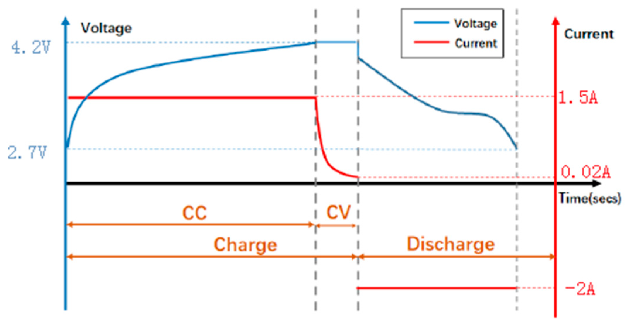
The voltage and current at a charge and discharge cycle is shown in Figure 1. And multiple charging and discharging cycles is to repeat the process until the batteries reached end-of-life (EOL) criteria, which was a 30% fade in rated capacity.
- (a)
- Charging process: Charging was carried out in a constant current model at 1.5 A until the battery voltage reached 4.2 V and then continued in a constant voltage model until the charge current dropped to 0.02 A.
- (b)
- Discharging process: Discharge was carried out at a constant current level of 2 A until the battery fell to 2.7 V for batteries #B5.
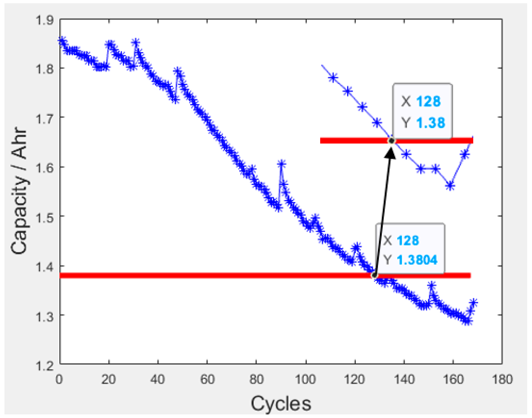
When the actual capacity of the lithium-ion battery drops to 70% of the rated capacity, that is, from 2 Ahr to 1.4 Ahr, the experiment stops, which means that the lithium-ion battery reaches the cut-off life point. The capacity decline curve of the #B5 battery is shown in the Figure 2.
The capacity degradation curve of lithium-ion batteries is obvious nonlinear, non-Gaussian characteristics, as shown in Figure 2. The battery is needed to be charged and discharged continuously, thus the capacity of the battery will degrade over time. Due to the good continuity of the capacity degradation trend, the actual capacity of the battery can be used to characterize the health status of the lithium-ion battery. Therefore, the end of life (EOL) of the lithium-ion battery can be defined as the number of discharge cycles when the actual capacity drops to the specified capacity threshold for the first time. For the sake of simplicity, the capacity threshold is defined as 1.38 Ahr, which is an integer multiple cycles and is near to 70% of the rated capacity.
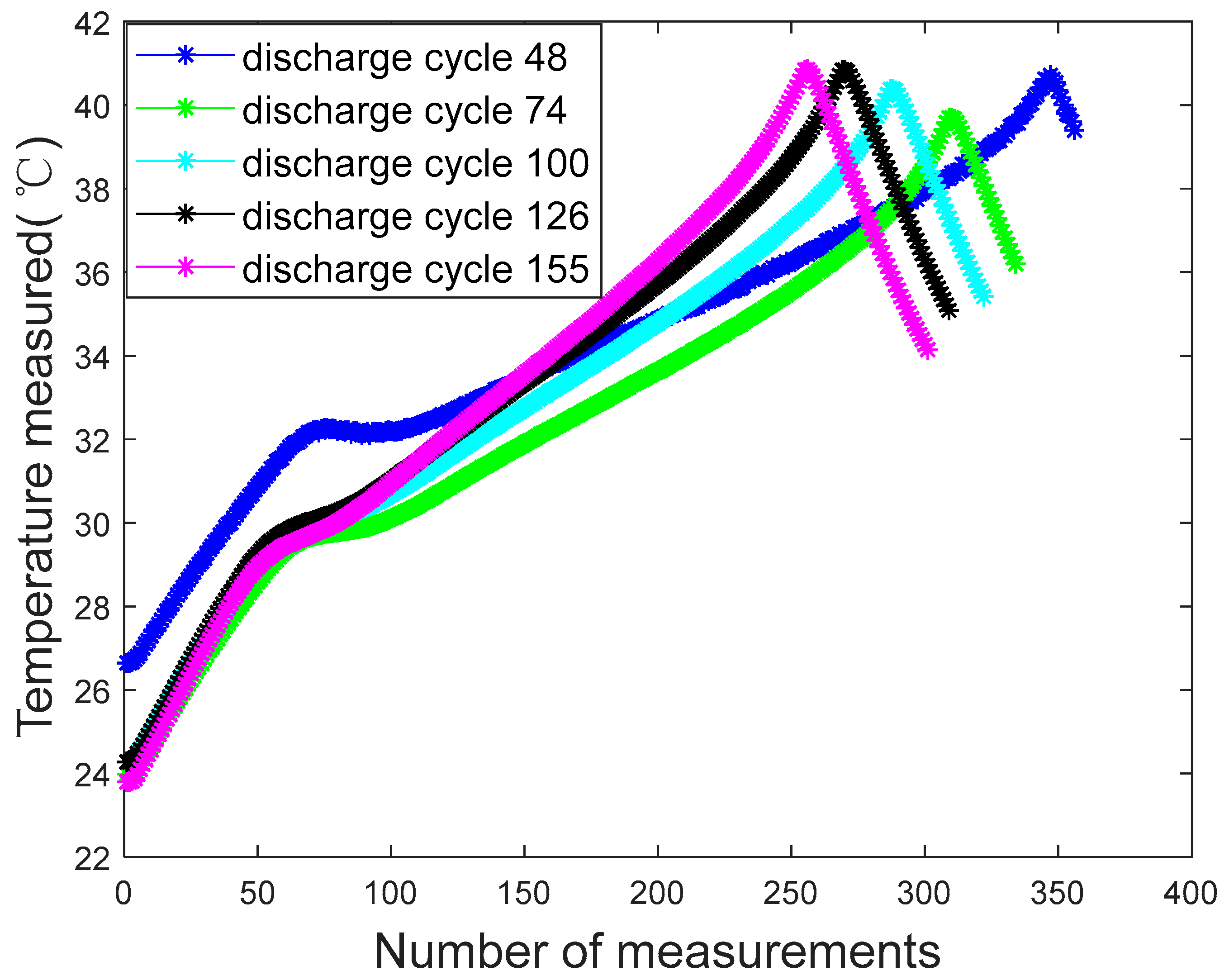
In addition, it will be interesting to observe that the temperature inside the lithium-ion battery changes with the charge and discharge cycle at room temperature (24 °C). As can be seen from the Figure 3, during the discharge process, the temperature of the battery gradually increased at first, then dropped quickly in the end.
2.2. Data Normalized
The input should be normalized by the follow formula:
where is the actual measured values; and are the minimum and maximum in the original sequence correspondingly; is the normalized value, which belong to .
2.3. Evaluation Index
In order to evaluate the prediction accuracy of the network model quantitatively, the absolute error, relative error and root mean square error of the lithium-ion battery RUL prediction can be used for analysis.
where EOP (end of prediction) represents the predicted battery end of life; RUL_ae represents the predicted absolute error; RUL_re (%) represents the predicted relative error; RMSE represents the root mean square error.
When the corresponding input and output of the network model are determined, one of the problems that comes with it is how to determine the number of hidden layers and the number of hidden layer nodes. In general, only the network structure with one hidden layer is considered, because firstly a network included one hidden layer with enough neurons can solve any finite input-output mapping problem; secondly, it is more difficult to increase the prediction accuracy by adding hidden layer than increasing the number of hidden layer nodes in actual training. At present, there is no accurate mathematical formula for the selection of the number of hidden nodes in the NN, and most of them are based on the following empirical model.
where represents the number of hidden layer nodes; represents the number of input layer nodes; represents the number of output layer nodes; is a constant between 1 and 10.
3. Different NN Models
3.1. The BP NN Model
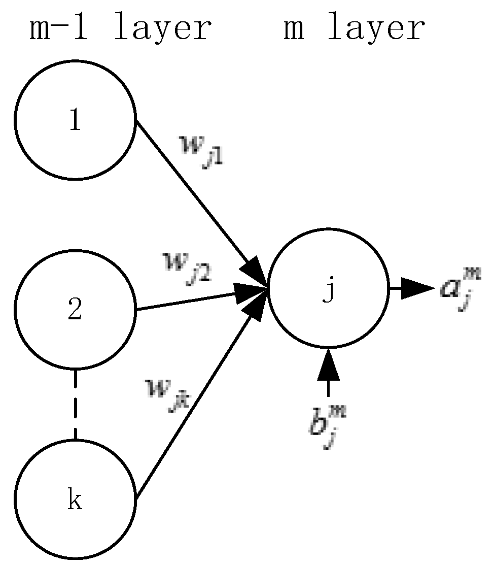
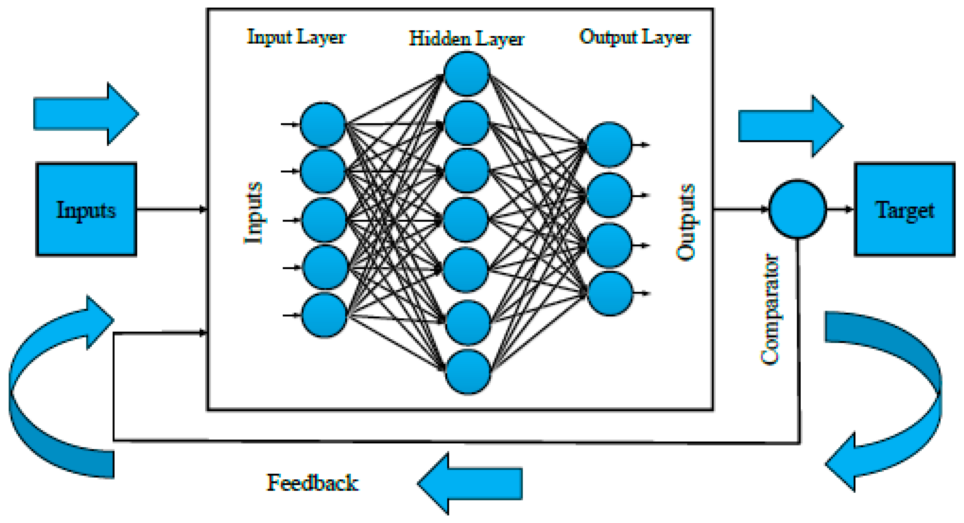
The BP NN belongs to a kind of multilayer feedforward NN. It advances layer by layer according to the weight coefficient during training, and it adjusts the weight and bias of the network dynamically based on the back propagation algorithm. Structurally, it consists of an input layer, an output layer, and a hidden layer; in essence, the BP algorithm uses the squared error sum of the network as the objective function and uses the gradient descent method to calculate the minimum value of the objective function. Its basic structure is shown in the Figure 4:
The neural model in Figure 4 can be expressed mathematically as,
where the input values of a node, , replicate the dendrites of the biological neuron and are multiplied by their respective connection weights, , and then summed. The summation is applied to the function of node , along with the bias , giving as a result the activation value of the node .
3.2. The NAR NN Model
The dynamic NN can add the data saved at the previous time to the calculation of the data at a later time through feedback and delay, so it is more suitable for the prediction of time series. Among them, the NAR NN is a kind of dynamic NN, which has been widely used in practical applications. Its basic structure is shown in Figure 5.
As can be seen in equation (5), the output is defined by , which indicates that the current value of the system is determined by past values.
3.3. The LSTM NN Model
In general, the time series prediction modeling is a difficult problem, because unlike regression prediction modeling, the interdependence between time series makes the problem difficult. As a kind of deep learning network structure, LSTM has the advantage that the context of data is considered in the training process. Compared with the traditional data-driven prediction method, the LSTM network has stronger nonlinear approximation ability. The general structure of the LSTM network is shown graphically in Figure 6.
There is a structure called “gate” in LSTM to remove or increase the ability of information to be passed to the memory unit. A gate is a structure that allows information to pass selectively. It consists of a sigmoid NN layer and a point multiplication operation. The sigmoid layer outputs a value between 0 and 1, describing how much of each part can pass. In a memory unit, there are three types of gates, namely a forgotten gate, an input gate, and an output gate, which are described in detail below.
Forget gate: . takes inputs of and , and outputs a number between 0 and 1 for each state . A = 1stands for retaining the state value completely, whereas A = 0 represents discarding the value completely. The forget gate is calculated as follows:
Input gate and input node: “input gate”, , decides which values to update. “input node”, , creates a new candidate state . The equations to calculate the two outputs are as follows:
Combing (6) and (7) to update the previous internal state into the current state :
Output gate: finally, there is a sigmoid layer called the “output gate”, , that determines what information to output. After putting the internal state through a tanh layer This can be implemented as:
where and are the layer weights and biases, respectively.
3.4. The Improved LSTM Model
The LSTM model selects the historical capacity data of the lithium-ion battery as an input variable to predict the remaining capacity of the lithium-ion battery in the future. Taking the #B5 battery as an example, the length of the capacity data is 168, that is:
The original capacity data is then divided into training sets and testing sets based on the predicted starting point T. The will be normalized by the methods presented in the previous parts and will be got, namely:
In the traditional LSTM prediction methods, and will be defined as the input and output to construct a LSTM model.
Since there are few data samples, a data construction method of the following form is proposed in order to achieve higher prediction accuracy and make the construction of the model simpler. Assuming that the width of the split window is L and m = T − 1, the input and output of the LSTM model can be expressed as:
where belongs to ; represents the normalized data sequence value; represents the input of the network; represents the output label of the corresponding input.
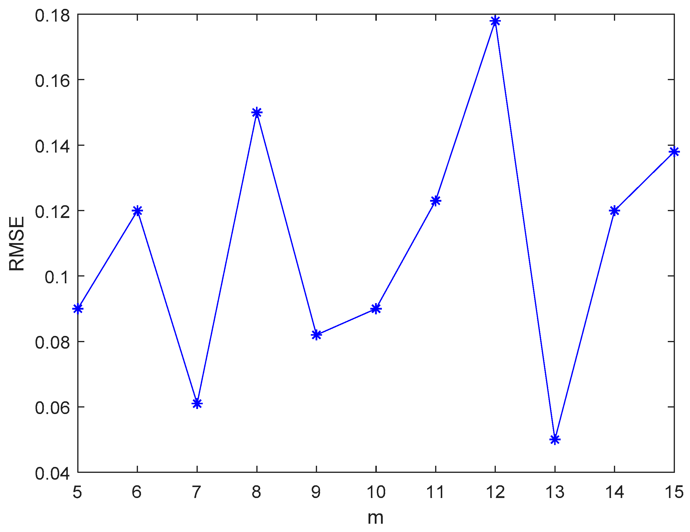
According to our lots of simulation experiments and relative references, the width of the split window is set 12, i.e., l = n = 12, thus m belongs to (5, 15) based on the data processing method in Equations (3) and (12). Under the same conditions, we have studied the variation of the RMSE of the LSTM network with m, as shown in the Figure 7. As can be seen from the Figure 7, when m is equal to 13, the root mean square error of the network is the smallest, so m = 13 in this paper.
4. Results and Discussion
The software package and the version used to implement all three NNs structures is MATLAB2018a. For the LSTM network model in this paper, according to our analysis and pre-experiments mentioned above, l = n = 12, m = 13, α = 8, the learning rate is set 0.005. The predicted starting point is set for #B5. The battery will be predicted 200 times at each prediction starting point and the point not reached failure threshold will be eliminated. Figure 8, Figure 9 and Figure 10 show the prediction results at three different prediction starting points.
The prediction result of LSTM at T1 = 69 is shown in Figure 8. As can be seen in the Figure 8, the prediction result is 124 and the relative error is−4.
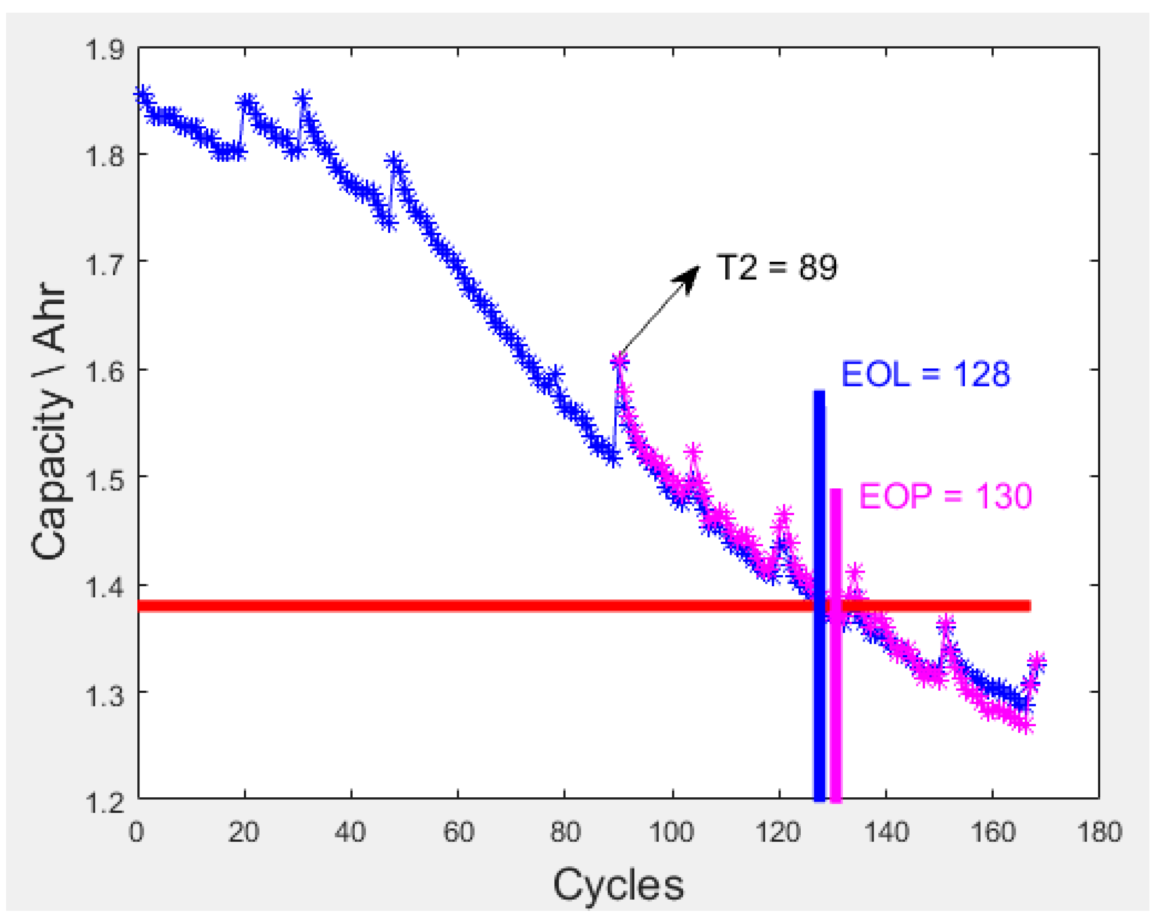
The prediction result of LSTM at T2 = 89 is shown in Figure 9. As can be seen in Figure 9, now the prediction result is 130 and the relative error is 2, which means that the prediction error is gradually decreasing.
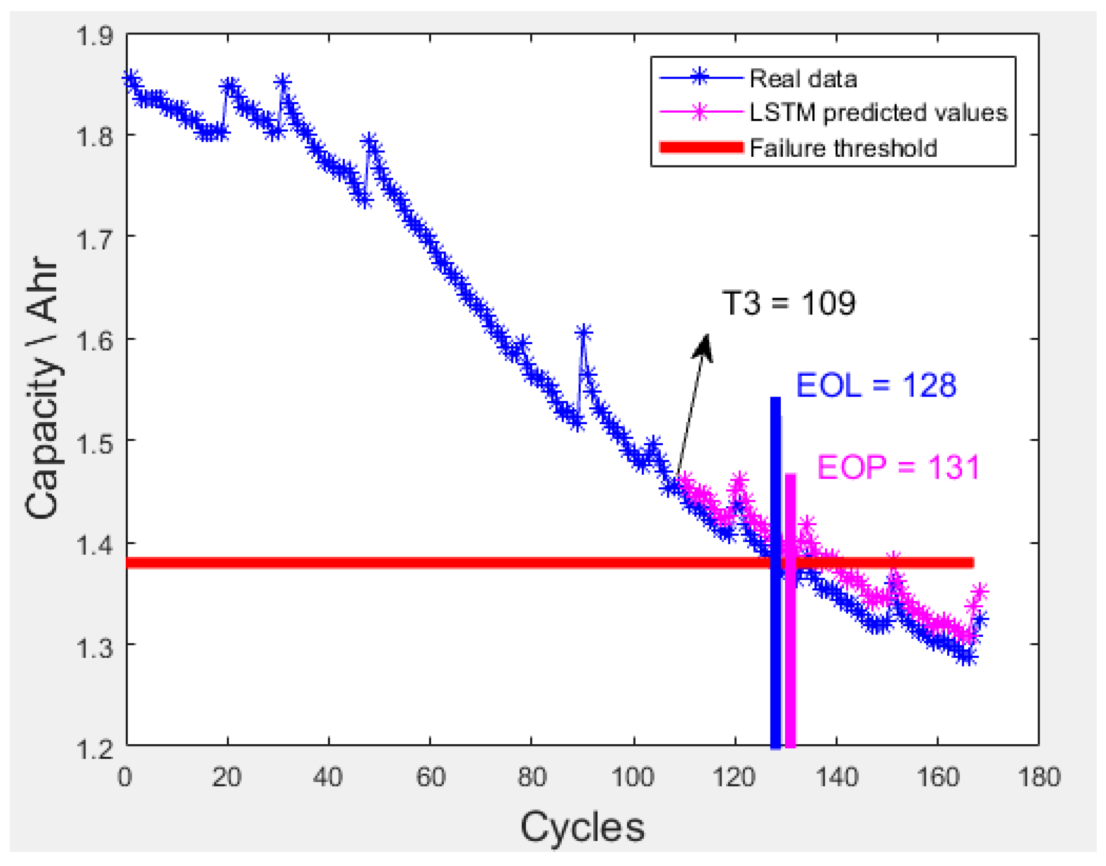
The prediction result of LSTM at T3 = 109 is shown in Figure 10. As can be seen in the Figure 10, the prediction result is 131 and the relative error is 3.
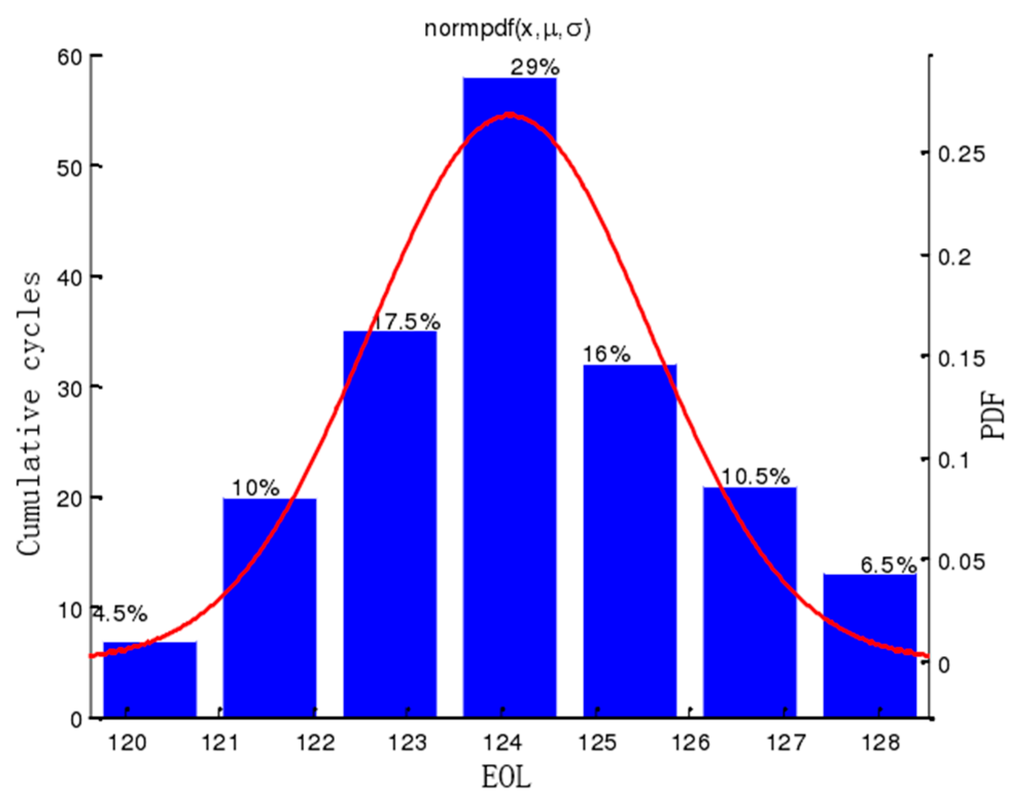
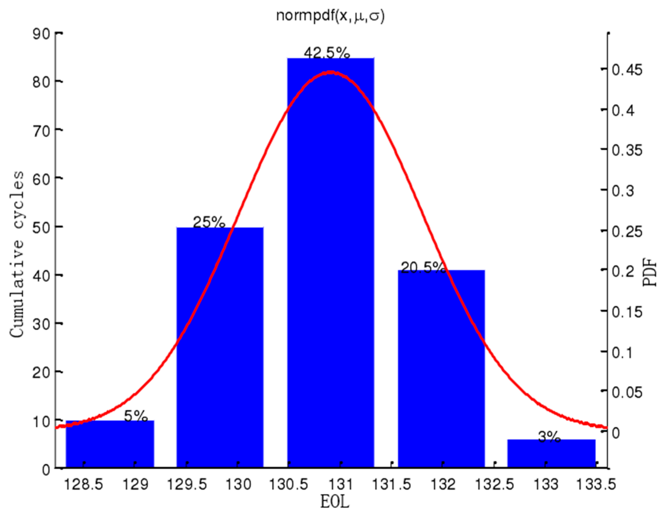
The LSTM model can achieve a good prediction accuracy of the lithium-ion battery capacity, as shown in Figure 8, Figure 9 and Figure 10. In order to observe the prediction effect of the LSTM model under different prediction starting points intuitively, the probability distribution histograms (PDH) of the #B5 battery prediction results at different prediction starting points is shown in Figure 11, Figure 12 and Figure 13.
The probability distribution histograms and the probability distribution curve of the LSTM model after 200 tests is shown in Figure 11. As can be seen in Figure 8 and Figure 11, due to the randomness of the network in initializing weights and bias, the prediction results are not same at each test, but the improved LSTM model proposed in this paper can approach the real life cut-off point of lithium-ion batteries with a high probability from the long-term prediction results, which verify the validity of the model.
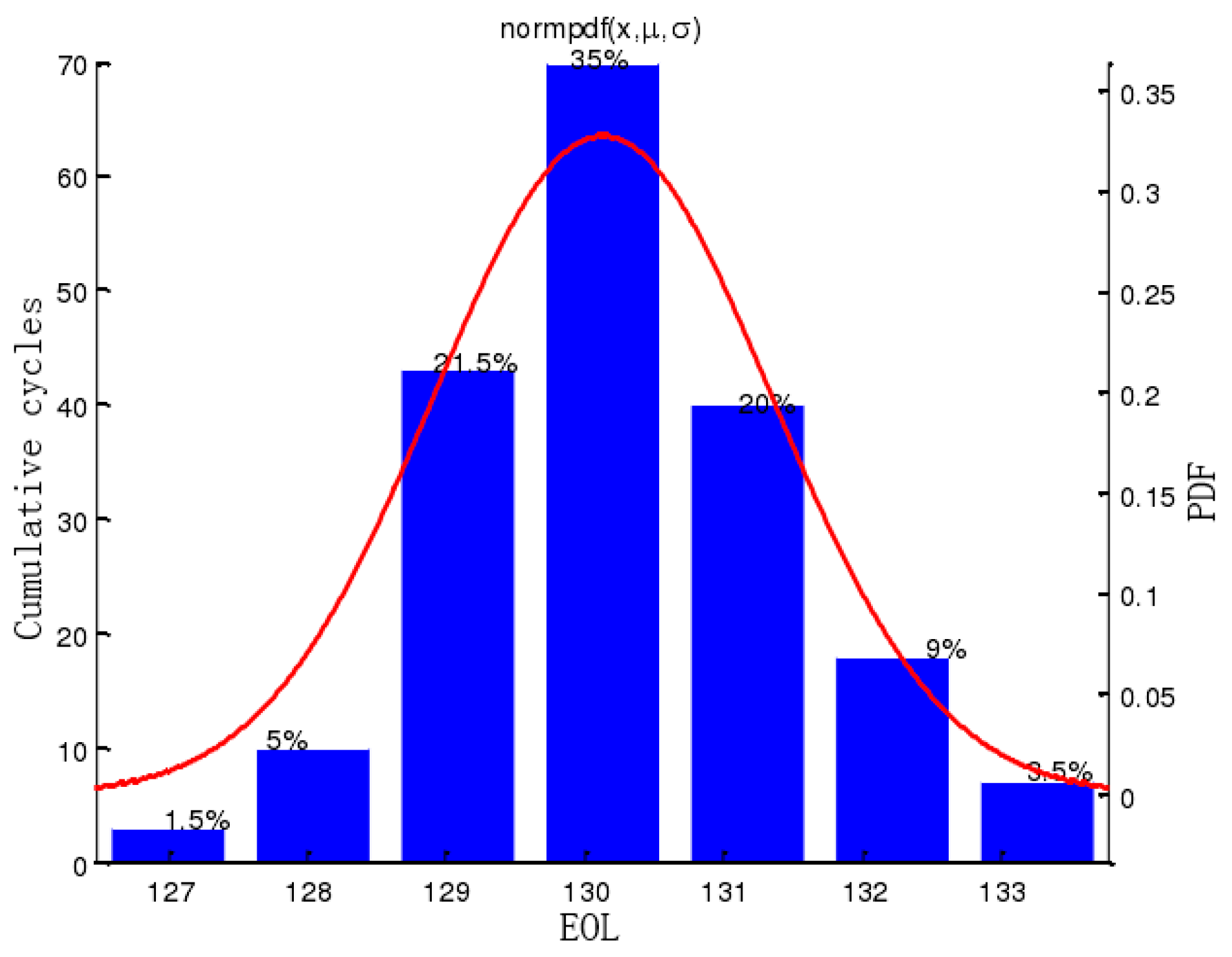
Figure 12 is similar to Figure 11, except that it is a statistical distribution of #B5 with the improved LSTM model after 200 tests at T2 = 89. As seen in Figure 12, the prediction result is 130, which is very close to the real life cut-off point of the lithium-ion battery.
From the probability distribution histogram of the prediction results, when we use 69, 89, 109 as the prediction starting point of the network to predict the remaining service life of the lithium-ion battery, the life expectancy cutoff point of the battery B5 is 124, 130, 131, respectively. The corresponding probabilities are 29%, 35%, and 42.5%, respectively. In addition, we can also see that the normal distribution probability density curve fitted by the prediction results becomes thinner and thinner with the increase of the prediction starting point, which indicates that the accuracy of the prediction is also gradually increasing.
In order to compare the prognostics of the lithium-ion batteries based on different ANN, such as BP, NAR, and LSTM, the comparison results of the three algorithms are shown in Figure 14 and Table 1. The parameters for LSTM and NAR are: n = l = 12, m = 13, α = 8, d = 20.
As can be seen from Table 1, among the three prediction algorithms, LSTM has the highest prediction accuracy. When 80, 90, and 100 are used as prediction starting points respectively, the corresponding absolute errors are 13, 8, and 2, and the relative errors are 10.16%, 6.25%, and 1.56%. From the absolute error, relative error and RMSE corresponding to the prediction results, the LSTM model is indeed more accurate than the static BP network and the dynamic NAR network. By comparing these three different prediction algorithms, we can know that the LSTM network is better for the time series problem of lithium-ion battery life prediction, and the learning ability of the degradation process is stronger. In addition, the NAR ANN has the better prognostic accuracy compared to the BP ANN.
5. Conclusions
An improved LSTM prediction method for lithium-ion battery RUL estimation is proposed in this paper. And the prognostics comparison of lithium-ion battery based on the BP ANN, the NAR ANN and the LSTM ANN has been studied in detail. The experimental results show: (1) compared with the static NN prediction model and the dynamic NN prediction model, the LSTM model based on the deep learning theory can achieve better dependence, lower prediction error and higher prediction accuracy; (2) the NAR ANN has the better prognostic accuracy compared to the BP ANN.
For lithium-ion batteries, the error and accuracy of the prediction results obtained by applying the LSTM model are different at different prediction starting points. By analyzing the prediction results of the B5 using the LSTM model, the more the predicted starting point is, that is, the more samples are trained, the higher the accuracy of the obtained network model, but the longer the training model takes, a balance needs to be struck between prediction accuracy and training time.
Author Contributions
Methodology, B.L.; software and writing original draft, X.L.; editing, X.G.; project administration, Z.L.
Funding
This work was supported in part by National Natural Science Foundation of China under Grants U1830133.
Acknowledgments
The authors would like to thank NASA Ames Prognostics Center of Excellence (PCoE) for their lithium-ion battery experimental data.
Conflicts of Interest
The authors declare no conflict of interest.
References
- Zhang, J.; Lee, J. A review on prognostics and health monitoring of Li-ion battery. J. Power Sources 2011, 196, 6007–6014. [Google Scholar] [CrossRef]
- Long, B.; Xian, W.; Jiang, L.; Liu, Z. An improved autoregressive model by particle swarm optimization for prognostics of lithium-ion batteries. Microelectron. Reliab. 2013, 53, 821–831. [Google Scholar] [CrossRef]
- Xian, W.; Long, B.; Li, M.; Wang, H. Prognostics of Lithium-Ion Batteries Based on the Verhulst Model, Particle Swarm Optimization and Particle Filter. IEEE Trans. Instrum. Meas. 2014, 63, 2–17. [Google Scholar] [CrossRef]
- Eom, S.W.; Kim, M.K.; Kim, I.J.; Moon, S.I.; Sun, Y.K.; Kim, H.S. Life prediction and reliability assessment of lithium secondary batteries. J. Power Sources 2007, 174, 954–958. [Google Scholar] [CrossRef]
- Williard, N.; He, W.; Hendricks, C.; Pecht, M. Lessons Learned from the 787 Dreamliner Issue on Lithium-Ion Battery Reliability. Energies 2013, 6, 4682–4695. [Google Scholar] [CrossRef] [Green Version]
- Vasan, A.S.S.; Long, B.; Pecht, M. Diagnostics and Prognostics Method for Analog Electronic Circuits. IEEE Trans. Ind. Electron. 2013, 60, 5277–5291. [Google Scholar] [CrossRef]
- Long, B.; Xian, W.; Li, M.; Wang, H. Improved diagnostics for the incipient faults in analog circuits using LSSVM based on PSO algorithm with Mahalanobis distance. Neurocomputing 2014, 133, 237–248. [Google Scholar] [CrossRef]
- Ren, L.; Zhao, L.; Hong, S.; Zhao, S.; Wang, H.; Zhang, L. Remaining Useful Life Prediction for Lithium-Ion Battery: A Deep Learning Approach. IEEE Access 2018, 6, 50587–50598. [Google Scholar] [CrossRef]
- Zhang, Y.; Xiong, R.; He, H.; Pecht, M.G. Long short-term memory recurrent neural network for remaining useful life prediction of lithium-ion batteries. IEEE Trans. Vehicl. 2018, 67, 5695–5705. [Google Scholar] [CrossRef]
- Gu, J.; Barker, D.; Pecht, M. Prognostics implementation of electronics under vibration loading. Microelectron. Reliab. 2007, 47, 1849–1856. [Google Scholar] [CrossRef]
- Miao, Q.; Xie, L.; Cui, H.; Liang, W.; Pecht, M. Remaining useful life prediction of lithium-ion battery with unscented particle filter technique. Microelectron. Reliab. 2013, 53, 805–810. [Google Scholar] [CrossRef]
- Zhang, X.; Miao, Q.; Liu, Z. Remaining useful life prediction of lithium-ion battery using an improved UPF method based on MCMC. Microelectron. Reliab. 2017, 75, 288–295. [Google Scholar] [CrossRef]
- Zhao, Q.; Qin, X.; Zhao, H.; Feng, W. A novel prediction method based on the support vector regression for the remaining useful life of lithium-ion batteries. Microelectron. Reliab. 2018, 85, 99–108. [Google Scholar] [CrossRef]
- Widodo, A.; Shim, M.-C.; Caesarendra, W.; Yang, B.-S. Intelligent prognostics for battery health monitoring based on sample entropy. Expert Syst. Appl. 2011, 38, 11763–11769. [Google Scholar] [CrossRef]
- Jia, B.; Guan, Y.; Wu, L. A State of Health Estimation Framework for Lithium-Ion Batteries Using Transfer Components Analysis. Energies 2019, 12, 2524. [Google Scholar] [CrossRef]
- Pang, X.; Huang, R.; Wen, J.; Shi, Y.; Jia, J.; Zeng, J. A Lithium-ion Battery RUL Prediction Method Considering the Capacity Regeneration Phenomenon. Energies 2019, 12, 2247. [Google Scholar] [CrossRef]
- Liu, J.; Saxena, A.; Goebel, K.; Saha, B.; Wang, W. An Adaptive Recurrent Neural Network for Remaining Useful Life Prediction of Lithium-Ion Batteries. In Proceedings of the Annual Conference Prognostics Health Management Society, Portland, OR, USA, 10–14 October 2010; pp. 1–9. [Google Scholar]
- Rezvani, M.; AbuAli, M.; Lee, S.; Lee, J.; Ni, J. A comparative analysis of techniques for electric vehicle battery prognostics and health management (PHM). SAE Tech. Pap. 2011. [Google Scholar] [CrossRef]
- Hochreiter, S.; Schmidhuber, J. Long short-term memory. Neural Comput. 1997, 9, 1735–1780. [Google Scholar] [CrossRef] [PubMed]
- Gers, F.A.; Schmidhuber, J.; Cummins, F. Learning to Forget: Continual Prediction with LSTM. Neural Comput. 2000, 12, 2451–2471. [Google Scholar] [CrossRef] [PubMed]
- Duan, Y.; Lv, Y.; Wang, F.Y. Travel Time Prediction with LSTM Neural Network. In Proceedings of the IEEE 19th International Conference on Intelligent Transportation Systems (ITSC), Rio de Janeiro, Brazil, 1–4 November 2016; pp. 1053–1058. [Google Scholar]
- Funaya, K.; Guo, T.; Xu, Z.; Yao, X.; Chen, H.; Aberer, K. Robust Online Time Series Prediction with Recurrent Neural Networks. In Proceedings of the IEEE International Conference on Data Science and Advanced Analytics (DSAA), Montreal, QC, Canada, 17–19 October 2016; pp. 816–825. [Google Scholar]
- Saha, B.; Goebel, K. Battery Data Set, NASA Ames Prognostics Data Repository; NASA Ames: Moffett Field, CA, USA, 2007. [Google Scholar]
Figure 1.
The voltage and current at a charge and discharge cycle.

Figure 2.
Capacity degradation curves of #B5.

Figure 3.
the battery temperature process change during the discharge cycle.

Figure 4.
The basic structure of the back propagation (BP) network.

Figure 5.
The structure of the nonlinear autoregressive (NAR) network.

Figure 6.
The structure of the long short-term memory (LSTM) network.

Figure 7.
the variation of the RMSE of the LSTM network with m.

Figure 8.
The prediction result of LSTM at T1 = 69.

Figure 9.
The prediction result of LSTM at T2 = 89.

Figure 10.
The predictions result of LSTM at T3 = 109.

Figure 11.
The probability distribution histograms (PDH) of LSTM prediction results at T1 = 69.

Figure 12.
The PDH of LSTM prediction results at T2 = 89.

Figure 13.
The PDH of LSTM prediction results at T3 = 109.

Figure 14.
The comparison of three prediction results.


Table 1.
the comparison of three algorithms of #B5.
| Algorithm | Origin | EOP | RUL_ae | RUL_re (%) | RMSE |
|---|---|---|---|---|---|
| BP | T1 = 80 | 152 | 24 | 18.75 | 0.0586 |
| T2 = 90 | 147 | 19 | 14.84 | 0.0394 | |
| T3 = 100 | 133 | 5 | 3.91 | 0.0233 | |
| NAR | T1 = 80 | 148 | 20 | 15.63 | 0.0493 |
| T2 = 90 | 138 | 10 | 7.81 | 0.0373 | |
| T3 = 100 | 123 | 5 | 3.91 | 0.0282 | |
| LSTM | T1 = 80 | 141 | 13 | 10.16 | 0.0352 |
| T2 = 90 | 132 | 4 | 3.12 | 0.0302 | |
| T3 = 100 | 130 | 2 | 1.56 | 0.0118 |
© 2019 by the authors. Licensee MDPI, Basel, Switzerland. This article is an open access article distributed under the terms and conditions of the Creative Commons Attribution (CC BY) license (http://creativecommons.org/licenses/by/4.0/).
Share and Cite
MDPI and ACS Style
Long, B.; Li, X.; Gao, X.; Liu, Z. Prognostics Comparison of Lithium-Ion Battery Based on the Shallow and Deep Neural Networks Model. Energies 2019, 12, 3271. https://doi.org/10.3390/en12173271
AMA Style
Long B, Li X, Gao X, Liu Z. Prognostics Comparison of Lithium-Ion Battery Based on the Shallow and Deep Neural Networks Model. Energies. 2019; 12(17):3271. https://doi.org/10.3390/en12173271
Chicago/Turabian StyleLong, Bing, Xiangnan Li, Xiaoyu Gao, and Zhen Liu. 2019. "Prognostics Comparison of Lithium-Ion Battery Based on the Shallow and Deep Neural Networks Model" Energies 12, no. 17: 3271. https://doi.org/10.3390/en12173271
Note that from the first issue of 2016, this journal uses article numbers instead of page numbers. See further details here.