Power Quality Disturbances Assessment during Unintentional Islanding Scenarios. A Contribution to Voltage Sag Studies †


Department of Electrical Engineering, Polytechnic University of Catalonia, ETSEIB - Av. Diagonal 647, 08028 Barcelona, Spain
*
Author to whom correspondence should be addressed.
†
This paper is a technically extended version of a conference paper entitled “A novel voltage sag approach during unintentional islanding scenarios: A survey from real recorded events”, presented at ICREPQ’ 19, Tenerife, Spain, April 2019.
Energies 2019, 12(16), 3198; https://doi.org/10.3390/en12163198
Submission received: 10 July 2019
/
Revised: 6 August 2019
/
Accepted: 14 August 2019
/
Published: 20 August 2019
(This article belongs to the Special Issue Analysis for Power Quality Monitoring)
Abstract
:This paper presents a novel voltage sag topology that occurs during an unintentional islanding operation (IO) within a distribution network (DN) due to large induction motors (IMs). When a fault occurs, following the circuit breaker (CB) fault clearing, transiently, the IMs act as generators due to their remanent kinetic energy until the CB reclosing takes place. This paper primarily contributes to voltage sag characterization. Therefore, this novel topology is presented, analytically modelled and further validated. It is worth mentioning that this voltage sag has been identified in a real DN in which events have been recorded for two years. The model validation of the proposed voltage sag is done via digital simulations with a model of the real DN implemented in Matlab considering a wide range of scenarios. Both simulations and field measurements confirm the voltage sag analytical expression presented in this paper as well as exhibiting the high accuracy achieved in the three-phase model adopted.
1. Introduction
Over the last decade, the increasing interest in power quality (PQ) monitoring is becoming a crucial task for distribution operators (DSOs) and, presently, is among the issues of major concern. Since the DNs supply power to the costumers, monitoring the occurring events has become essential; therefore, presently, smart meters allocated in each customer node are playing a pivotal role [1,2]. Regarding the measurement and monitoring of PQ disturbances, several standards have been published within the EN-61000 series; these standards fall within the electromagnetic compatibility field. Particularly, EN61000-4-30 defines how to measure PQ disturbances and the measurement accuracy of the equipment and defines different classes of accuracy. A relevant summary and interpretation of these standards are given in References [3,4,5]. Furthermore, other research has been focused on how to identify the different type of disturbances from occurring events; for instance, in References [6,7,8,9,10,11]. Once PQ disturbances are detected, classifying them and compressing them into separate events is a challenging task and requires advanced tools; see References [12,13,14,15]. Some authors have considered fuzzy logic or neural networks to classify them [16,17,18,19], some others proceed based on clustering the data depending on its origin from offline and prescribed events [20,21], and lastly, certain studies have focused on real-time classification, which results in a successful classification; for instance, see References [22,23,24].
It is understood that PQ is one of the major concerns for DSOs, and probabilistic studies have been carried out to evaluate the grid reliability with statistical and stochastic assessments [25,26,27,28,29]. Such studies have concluded that protective devices and the weakness of the grid as well as the type of loads are crucial factors when carrying out PQ studies. Besides, with the growing interest in distributed generation (DG) and smart grids, their influence on the PQ field is currently under investigation [30,31,32]. It is also important to underline the importance of the PQ reliability indicators; for example, see the evaluations carried out in Reference [33,34,35,36,37,38].
All PQ disturbances are summarized in the standard EN-50160 (see Reference [39]). This standard defines all voltage disturbances as two types: (i) continuous phenomena (e.g., long-time disturbances in the range between ms and minutes), such as voltage drops, voltage swells or frequency oscillations; and (ii) short-duration disturbances such as voltage interruptions, voltage sags, voltage swells, and over-voltage transients (e.g., short-term disturbances in the range between μs to ms). An excellent review of PQ disturbances classification can be found in References [39,40].
Among all PQ disturbances, voltage sags have been the object of study for many years. At first, voltage sags were assumed to be rectangular. Afterwards, it was demonstrated that this was not strictly true, and the type of recovery, as well as the phase-angle-jump, played a significant role [41]. It is relevant to highlight the characterization done by Bollen in Reference [33], as well as in Reference [42]. Furthermore, immunity tests and studies of electrical devices’ behavior towards voltage sags have been thoroughly analyzed in References [43,44,45,46], where the effects of the voltage sags are evaluated. In this direction, several standards have been published; for instance, EN 61000-3-2 (limits for harmonic current emissions, less than 16 A), EN-61000-4-34 (immunity test for high current equipment, more than 16 A), and voltage sags with statistical results are summarized in IEC-61000-2-8. Considering that electrical device sensitivity is an aspect of utmost importance, immunity tests for voltage sags and interruptions are still under study.
Even though standard indices for reliability such as standard average interruption frequency index (SAIFI), standard average interruption duration index (SAIDI) or the reliability curves published by the information technology industry council (ITIC) have been defined, each country has its own regulations regarding the number of interruptions or their duration [47,48]. To deal with voltage sags effects, well-known equipment such as dynamic voltage restorers or an uninterruptible power supply are used [49,50], or even the use of FACTS [51].
Mainly, the origin of voltage sags in DNs and transmission networks (TNs) are faults; given their random nature in time and location, their magnitude, type and recovery can change along the grid. A fault in the system can produce either a voltage sag or an interruption, depending on where the fault originates; that is, depending on the type of network and configuration which is feeding the fault. Thereby, if several lines are feeding the fault, and if we assume that each one has its own CB, the faulted line/section will experience an interruption, whereas the adjacent section will experience a voltage sag. Commonly, the DN configuration is radial (i.e., there is only one source); therefore, if a fault appears and no DG is considered, the only source is the main grid. Therefore, costumers located downstream of the CB will experience a voltage sag during the fault, and once it is cleared, a supply interruption is expected. It will be demonstrated that the last assumption in the presence of large IMs may not be strictly true because an unintentional IO can occur before the CB reclosing.
As a matter of fact, this unexpected IO is the guiding principle of the voltage sag studied in the present paper. The unintentional IO begins once a fault is cleared and ends when the CB recloses to restore the electrical supply; typically, this reclosing time in DNs is between 500 ms and 1 s. Once the fault is cleared, transiently, IMs act as generators due to their remnant kinetic energy until the CB recloses the circuit. This phenomenon is partially analyzed in bus transfer during industry operations; for example, see Reference [52]. To achieve seamless transitions in this fast bus transfer, a microprocessor-based scheme has been implemented in Reference [53]. Nevertheless, none of these studies has considered the produced IO in the DN due to the IMs, on which the current PQ assessment is focused. Therefore, this paper makes a contribution to voltage sag characterization studies.
The paper is structured as follows: Section 2 reviews the present voltage sag characterization. In Section 3, the main features of the proposed voltage sag are detailed as well as its analytical expression. Section 4 shows the test system under investigation and the three-phase Matlab/Simulink model adopted. Section 5 displays the simulation results derived from the model. Section 6 discusses the model validation comparing the analytical form presented in Section 3, with both simulation results and field measurements. Lastly, Section 7 summarizes the main conclusions of the paper.
2. Voltage Sag Review
2.1. Introduction
Since voltage sags are a short-duration reduction of the root-mean-square (RMS) voltage, it can be said that their characterization depends on (i) their magnitude (i.e., voltage characteristic), (ii) their duration, (iii) their type, (iv) the type of recovery, (v) the phase-angle-jump, and (v) their origin. Nevertheless, the origin of the voltage sag will, in fact, dictate its type and its recovery. Moreover, voltage sags can change their type and become evolutionary voltage sags because the fault conditions can change (i.e., faults can evolve from one type of fault to another during the same event). Other parameters such as the point-on-wave in both the initiation and the recovery have been the object of study in Reference [54]. Besides this, an interesting analysis is done by Bastos et al. in Reference [55].
On the other hand, the data extracted from a measured sag are gained from the sag type characteristic voltage (i.e., the complex voltage) and by the positive–negative factor as published in References [56,57]. Particularly, according to Reference [56], there is a need to compress the three-phase voltage sag event into a single event, which is still under study by the IEEE project group P1159.2. Furthermore, a two-type contribution has been made in Reference [57], considering a three-phase–three-angle method. To obtain the main characteristics from a measured voltage sag, relevant methods are available in the literature, among which are the following:
- Complex voltage: This method uses symmetrical components to evaluate the type of sag; thus, comparing the angle between the definite sequence and the negative sequence, the sag type is obtained. The voltage characteristic is computed with the complex sum and difference of the positive and negative sequence-voltage.
- RMS voltage: These algorithms use the RMS voltage as input; thus, the computation of the six RMS values of the phase-to-phase and phase-to-neutral voltages is proposed. Therefore, the voltage characteristic, the voltage sag type and the positive-negative factor are extracted from these six voltage time-domain values.
- Advanced features: Within this group, a considerable number of articles have been published, and the main aim is to extract features from the voltage waveform considering a wide range of measurements and classify them with an algorithm that helps to compress the data. From all studies, the most appropriate methods are summarized in Reference [58]. Furthermore, Cai et al. in Reference [59] developed a mapping strategy for multiple disturbances.
In Reference [40], the authors focus on voltage sag characterization; thus, a general distinction is made considering balanced and unbalanced voltage sags originating from faults (i.e., short-circuits). Nonetheless, in this study, other sources of voltage sags, such as induction or synchronous motors during their starting process, are considered. Moreover, a further classification is included in Reference [60], where the voltage sag produced during transformer energization is evaluated.
Previously, in faults originated by short-circuits, between the fault inception and the fault recovery, the voltage characteristic has been considered constant; see Figure 1. However, this voltage characteristic may not be constant during the voltage sag; for instance, see Figure 3 of Reference [61]. One reason for this voltage characteristic increasing or decreasing during the fault could be that the impedance seen from the source changes during the disturbance. Another cause for a decrease in the residual voltage during the voltage sag can occur in the presence of IMs. In such a way, immediately following a fault, the IMs tend to contribute towards the fault (e.g., roughly one or two cycles) so that the drawn current decreases in time and the voltage value also decreases; this phenomenon is thoroughly detailed in Reference [62].
To summarize, the studied sources of voltage sags are listed as follows:
- Short-circuits (constant retained voltage);
- Motors start—either synchronous or induction motors (non-constant retained voltage);
- Transformer energization (non-constant retained voltage);
- Short-circuits in the presence of IMs (non-constant retained voltage);
- Sudden load changes—e.g., composite load connections (non-constant retained voltage).
2.2. Voltage Sag Main Features
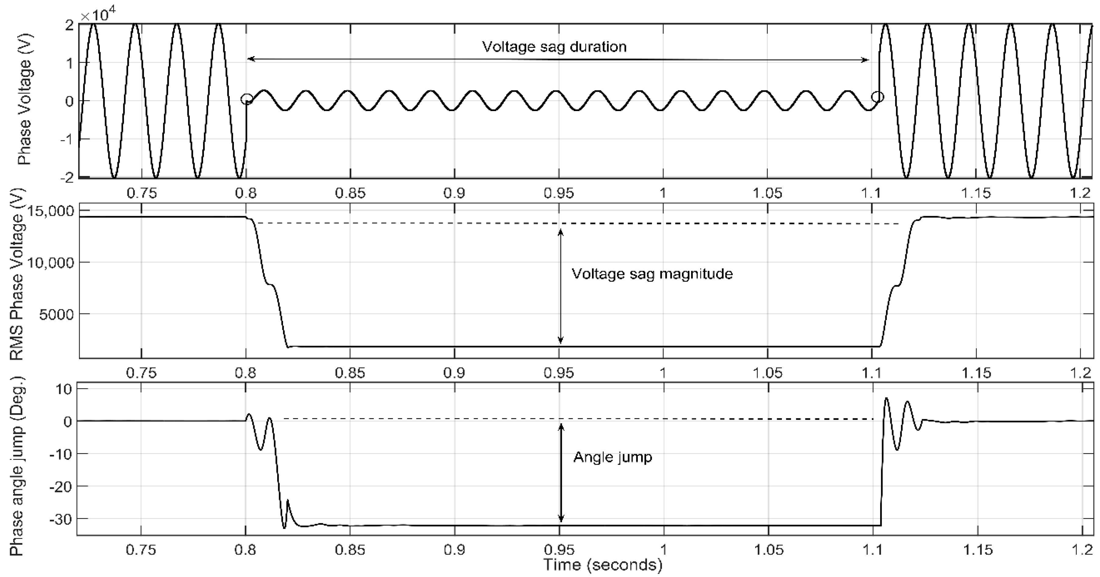
This subsection will show the main characteristics of voltage sags graphically in order to compare these parameters with the proposed voltage sag of the subsequent Section 3. Although the voltage sag representation of Figure 1 is not innovative, this figure and its analysis are necessary to highlight the improvement made with the proposed voltage sag as the object of study.
In Figure 1, the three principal magnitudes are shown in different plots. The first plot depicts the phase voltage waveform of the faulted phase. In this waveform, the beginning and the end of the fault can be observed as well as the point-on-wave in both the initiation and clearing (these two points are within two circles in the voltage waveform). The retained voltage—that is, the magnitude of the voltage sag—is shown in the second plot of Figure 1, and lastly, the phase-angle-jump is observable in the third plot of the same figure. For this particular event, the duration is 300 ms, and it originated due to a single-line-to-ground fault (SLG), which belongs to voltage sag type A in the characterization done by Bollen [63], the retained voltage is 0.12 pu, and the phase-angle-jump is −30 degrees, which means that the grid is predominantly inductive.
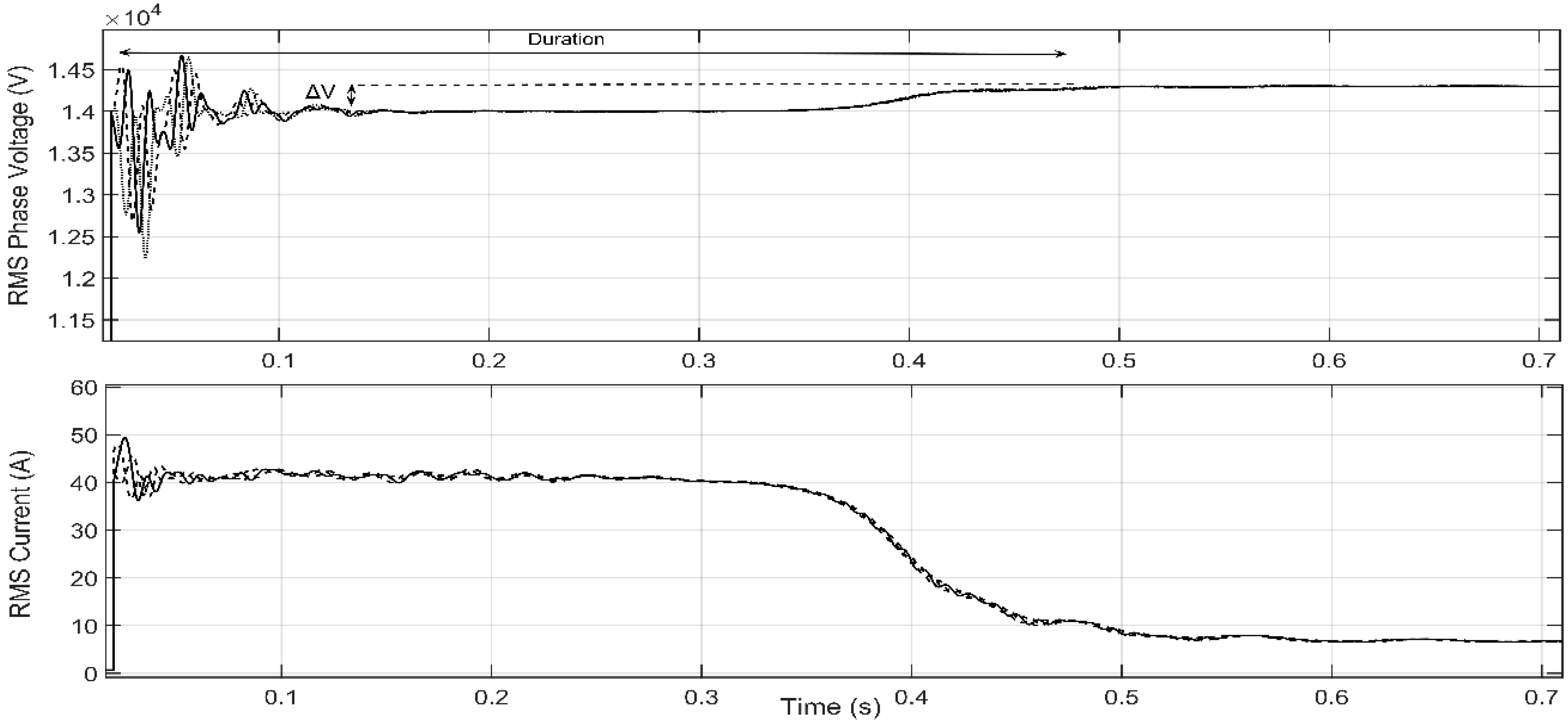
Figure 2 show the voltage sag produced by IMs starting; in this case, a group of 4 IMs of 160 kW have been simulated (all the IM data are detailed in Appendix A). It can be seen that the duration of the event is 500 ms, the voltage depth is 0.96 pu, and the voltage sag is balanced. In these cases, the strength of the grid plays a pivotal role. The first plot depicts the RMS phase voltage, and the second depicts the current.
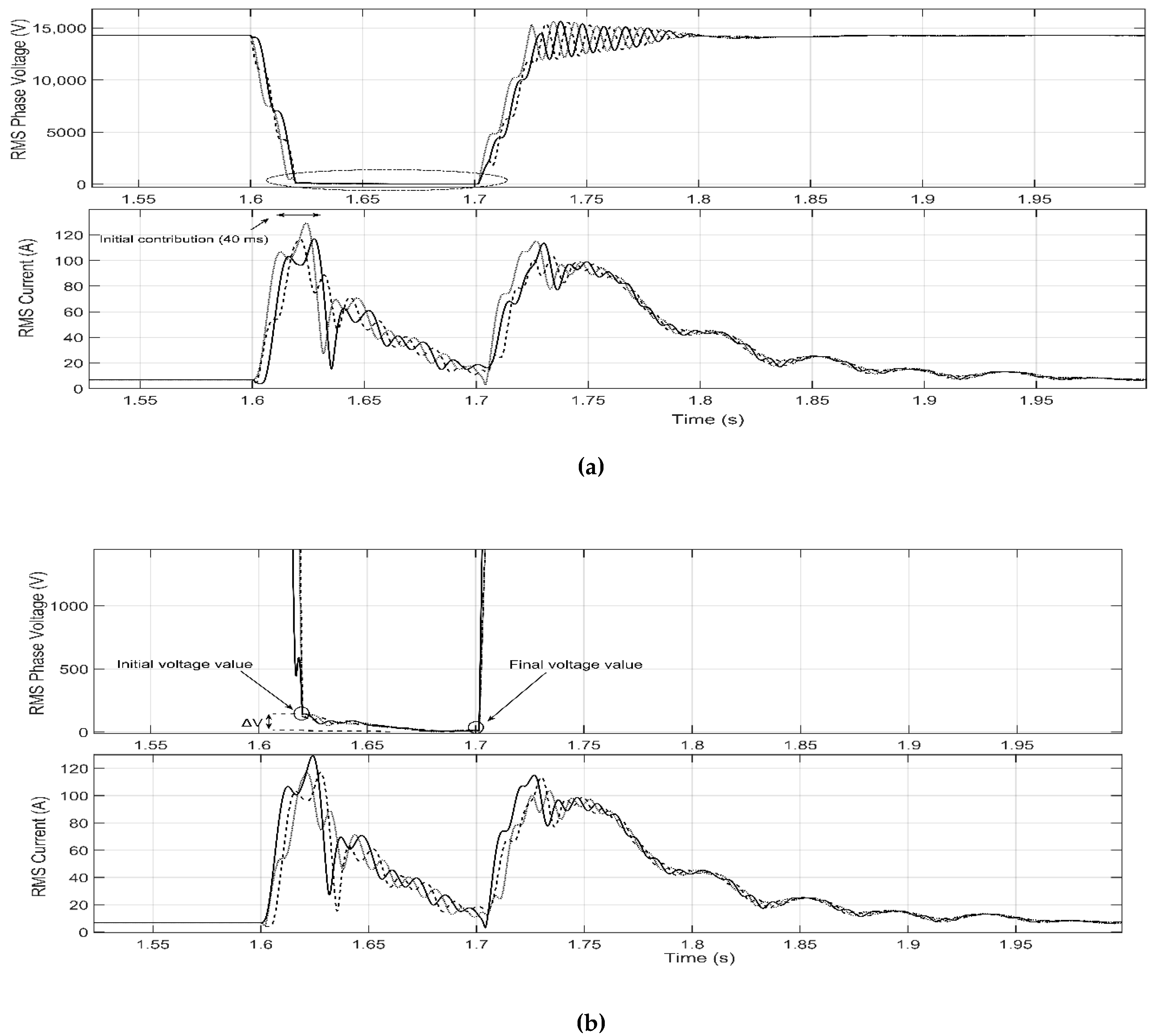
In Figure 3a, an example of the voltage sag produced when an IM contributes to a three-phase fault is shown. In the figure, the three-phase fault (Type A) is plotted. Nevertheless, to properly observe the voltage variation, in Figure 3b, the voltage sag is enlarged. In this figure, the decrease in the voltage characteristic during the event can be observed.
This voltage reduction during the voltage sag is due to the brief IM contribution towards the fault, which starts at t = 1.62 s, and in 2 cycles, the current starts to decrease. In these cases, the voltage variation due to this effect is ΔV = 125 V.
Taking into consideration that the loss of speed during the fault is low, the voltage sag due to the post-fault reacceleration is negligible (see the voltage characteristics between t = 1.7 s and t = 1.9 s in Figure 3a).
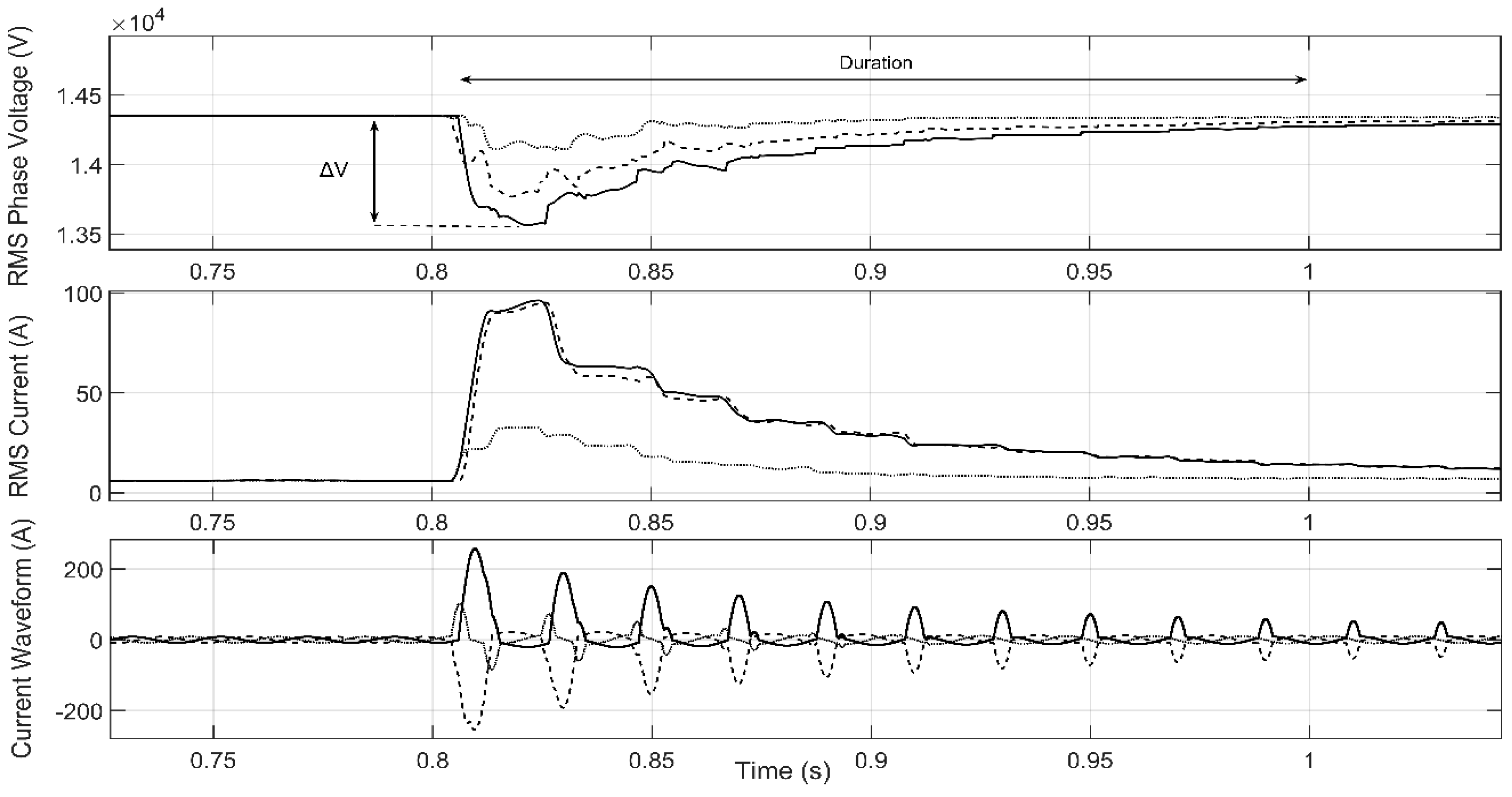
Figure 4 depicts the voltage sag produced when a transformer is energized; due to the current drawn by the transformer, transiently, the voltage drops to 0.94 pu. As can be seen, the voltage characteristic is not constant; it reaches a minimum value at t = 0.82 and starts to increase until t = 1s when the voltage sag is absolutely recovered. This voltage sag is unbalanced due to the current unbalance produced by the high content of current harmonics. Observing the third plot of Figure 4, the high content of harmonics of the current waveform can be seen; these harmonics are a direct consequence of the transformer core saturation [64].
To summarize, in this section, voltage sags with constant and non-constant retained voltage have been evaluated, which helps to clarify the voltage sag topology presented in this paper.
3. Voltage Sag Modelling
3.1. General Overview
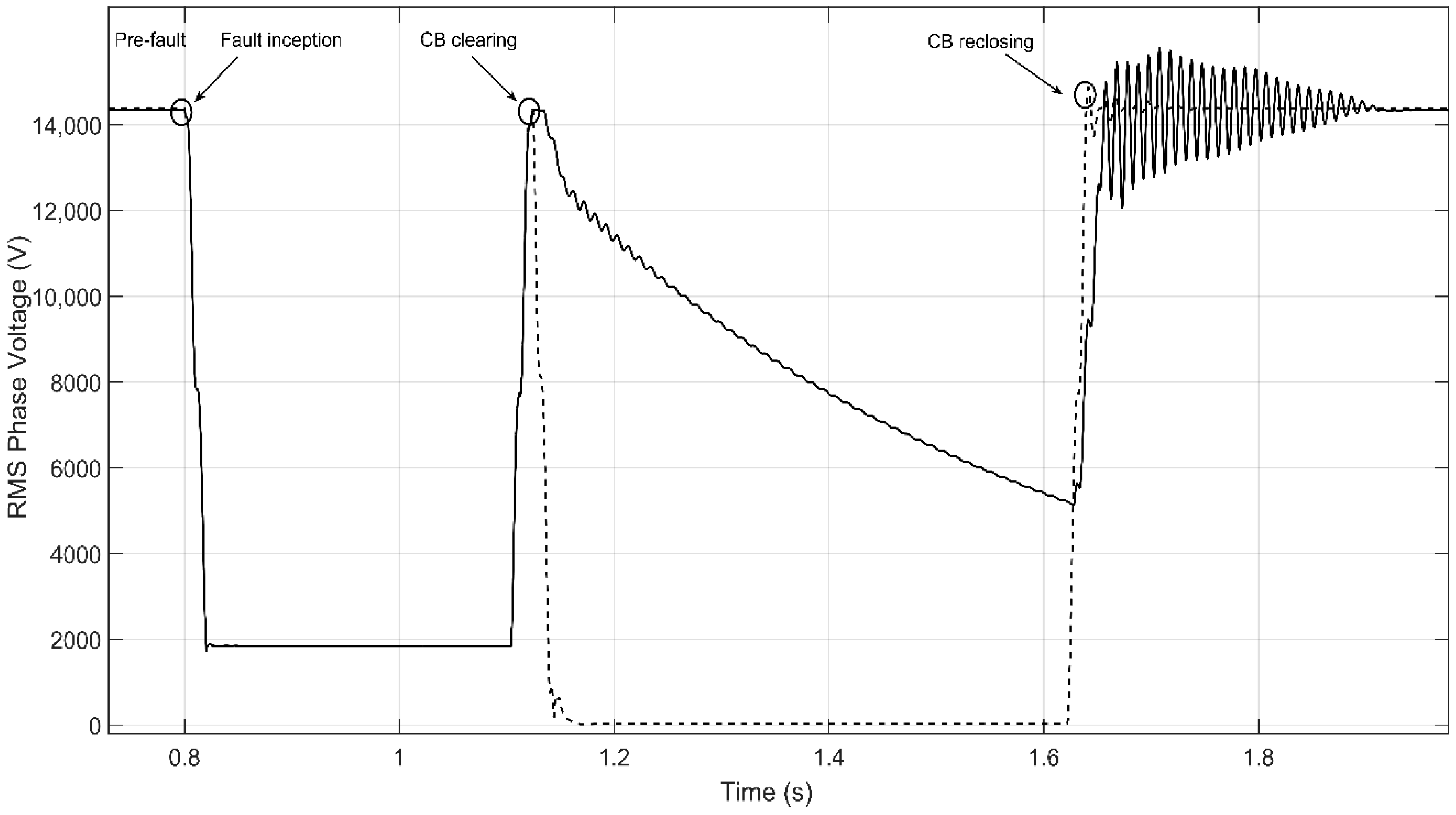
The current section is divided into four parts. The first introduces a general overview of the proposed voltage sag, the second analyses the analytical expression that follows the voltage sag magnitude, the third part examines its duration, and finally, the fourth part focuses on the recovery process once the CB recloses the circuit. Before the voltage sag modelling guidelines are analyzed in the further subsections, to observe the importance of this phenomenon clearly, Figure 5 shows the difference between one scenario with IMs and another one with the same rated apparent power when removing the IMs.
As can be seen in Figure 5, during the process between the clearing time (t = 1.1 s) and the CB reclosing (t = 1.6 s), in the case in which high IMs are present, a voltage sag appears. Meanwhile, when the IMs are removed, as expected, an interruption occurs.
3.2. Voltage Sag Magnitude: Analytical Expression
The analytical expression that follows the voltage sag during the island is, in fact, the IM stator voltage, which in turn depends on the stator current and its mechanical speed. Therefore, to obtain this expression, the IM equations have to be recalled. In a steady state, the IM acts as a motor and is being supplied by the grid and running at a specific point of operation. This point of operation is defined by the slip, the mechanical load torque coupled with the rotor shaft and the mechanical speed. These parameters dictate the initial kinetic energy of the machine before the fault appears. When a fault occurs, depending on the characteristics of the originated voltage sag (i.e., voltage sag magnitude and duration), the IM will lose speed according to this severity. Once the CB clears the fault, IMs, due to their stored kinetic energy, transiently act as generators. The pre-islanding conditions will dictate the voltage sag magnitude during the IO. Hence, the IMs’ initial kinetic energy is expressed as Equation (1)
where EKin_initial is the initial kinetic energy prior to the CB opening, JT is the total moment of inertia (considering the rotor inertia and mechanical load) and ωpre_islanding is the mechanical speed before the island is formed. The IM set of electrical equations are considered in stator reference and expressed in Park’s transformation to avoid the dependence of the coupling inductance with the mechanical angle θm Equations (2)–(5):
where V and i represent the voltage and current, respectively, M is the coupling inductance, L represents the inductance of the windings, ωm is the mechanical speed, ψ is the reference angle (stator reference in this case), is the IM pole pairs, θm is the rotor angle, the sub-indices s and r denote stator and rotor, respectively and dq refers to the direct and quadrature components of the Park’s transformation. The relation between abc and dq can be expressed as in Equation (6)
Following the CB opening, due to the lack of supply, the equilibrium between torques is broken, its speed derivative becomes negative, and therefore only the dynamic torque drives the machine. Moreover, the feeder loads which remain within the island represent a load torque for the IMs when acting as generators. Thereby, the electrical loads act as a torque decelerating the machines. The mechanical expressions acting as generators once the IMs are removed from the grid are computed as Equations (7) and (8):
where Γem is the electromagnetic torque, Γb is the friction torque, Γres is the mechanical load torque, θm is the angular position, JT is the total moment of inertia (considering the rotor inertia and mechanical load), and Γeload represents the equivalent torque developed by the feeder-load electrical power. If we consider load voltage dependence, constant impedance and constant current load models have to be considered; thereby, electrical loads are divided into P1, which is assumed to be the sum of all constant impedance loads, and P2, the sum of all constant current loads within the island. It follows that
where the sum of all constant impedance and constant currents considering n low voltage (LV) nodes is computed as Equation (10):
By integrating the IM speed derivative and mechanical angle with respect to time (7) and (8) during the island, the temporal evolution of ωm (t) and θm (t), are given by Equations (11) and (12):
where ti is the instant when the CB opens and tf when the CB recloses. Similarly, by integrating the current derivatives with respect to time in Equations (2)–(5), the temporal evolution of isd(t), isq(t), ird(t), and irq(t) is given by Equations (13)–(16):
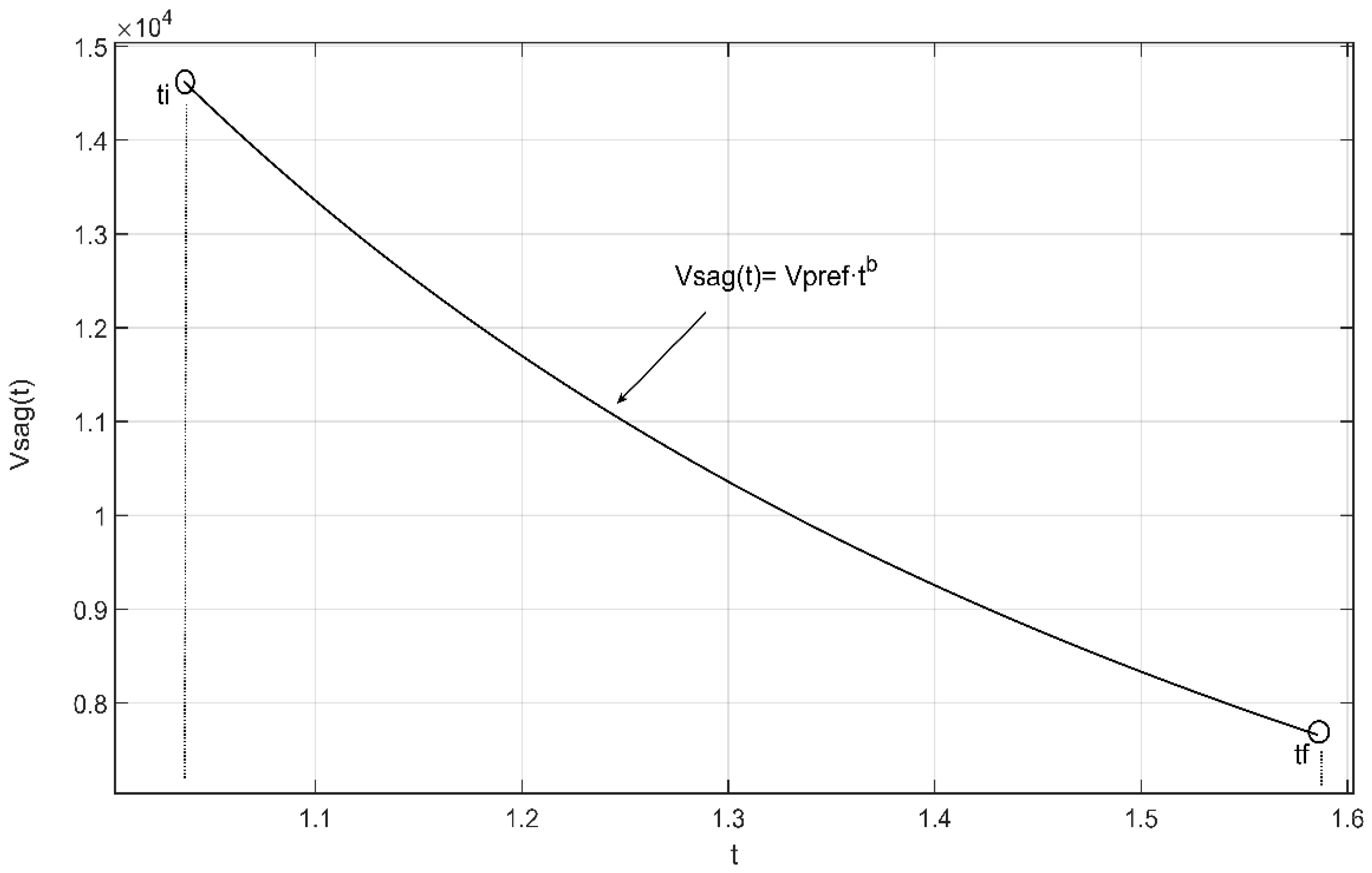
By solving the described set of Equations (11) and (12) and Equations (13)–(16) between ti and tf, the function that follows the voltage sag with respect to time is given by the IM stator voltages Vsd and Vsq. Furthermore, by solving Equations (11) and (12), one can observe that the IM mechanical speed decays exponentially due to the lack of supply; as a consequence, this decay is also observed in the stator voltages. Since the voltage sag magnitude is given by the IM stator voltage, its function has to be a negative exponential. In such a way, the voltage sag analytical expression with respect to time follows:
where Vsag(t) is the RMS phase voltage value, Vpre_fault is the RMS pre-fault phase voltage value, and b is a non-dimensional coefficient. Given the natural tendency of the IM to decelerate due to the lack of grid supply, this coefficient has to be below zero. Note that b values close to zero correspond to low loaded feeders, whereas large negative b values correspond to large loaded feeders. Figure 6 plots the function that follows the analytical expression for a given b value. It is crucial to highlight the fact that, as mentioned earlier, the analytical expression of the voltage sag magnitude is given by the IM stator voltages, which result from solving the differential Equations (11)–(16). Therefore, the b factor of Equation (17) can be obtained after this set of equations have been solved. Hence, Equation (17) provides a general expression to model this voltage sag which is performed after solving the differential equations of the system. Note, however, that depending on the terms in Equation (11) (i.e., the feeder-load power, the load torque and the friction torque), several b values can be obtained. Particularly, in Figure 6, ti = 1.04 s, tf =1.54 s and b= −1.52. It is relevant to highlight the fact that, as discussed above, this curve expression is only valid between ti and tf, where in fact the voltage sag characteristic is of interest.
3.3. Voltage Sag Duration
Voltage sag duration is defined as the period between the fault inception and the fault clearing; see the first plot of Figure 1. The voltage sag duration depends directly on the protective device’s settings. Particularly for the voltage sag described here, the voltage sag duration depends on the preset reclosing that takes place after a fault is cleared. This preset reclosing operation is widely implemented in DN relays, principally to avoid the need to operate the CB for non-permanent faults manually (e.g., self-extinguished faults). Commonly, DSOs set the first reclosing between 0.5 and 1 s.
3.4. Voltage Sag Recovery
Voltage recovery takes place at the instant when the CB clears a fault, as previously mentioned; depending on the type of voltage sag, it can be either abrupt (one stage recovery) or discrete (multi-stage recovery). Nonetheless, in the present voltage sag topology, the recovery is dictated by the CB reclosing following a preset time after the CB clearing. It is worth pointing out that, in this case, unlike the recovery due to short-circuits, the recovery can be defined in two steps.
The first step is due to the CB zero-crossing, which has to occur at the same instant for the three-phases, and the second is the recovery until the voltage reaches the pre-fault value. In fact, this is due to the high current drawn by the IM as a result of the out-of-phase reclosing and the subsequent IM reacceleration. The transient due to the out-of-phase reclosing is dictated by the difference in voltage amplitude between the grid and islanding as well as by the difference in frequency between the grid and islanding [52].
4. System Under Investigation
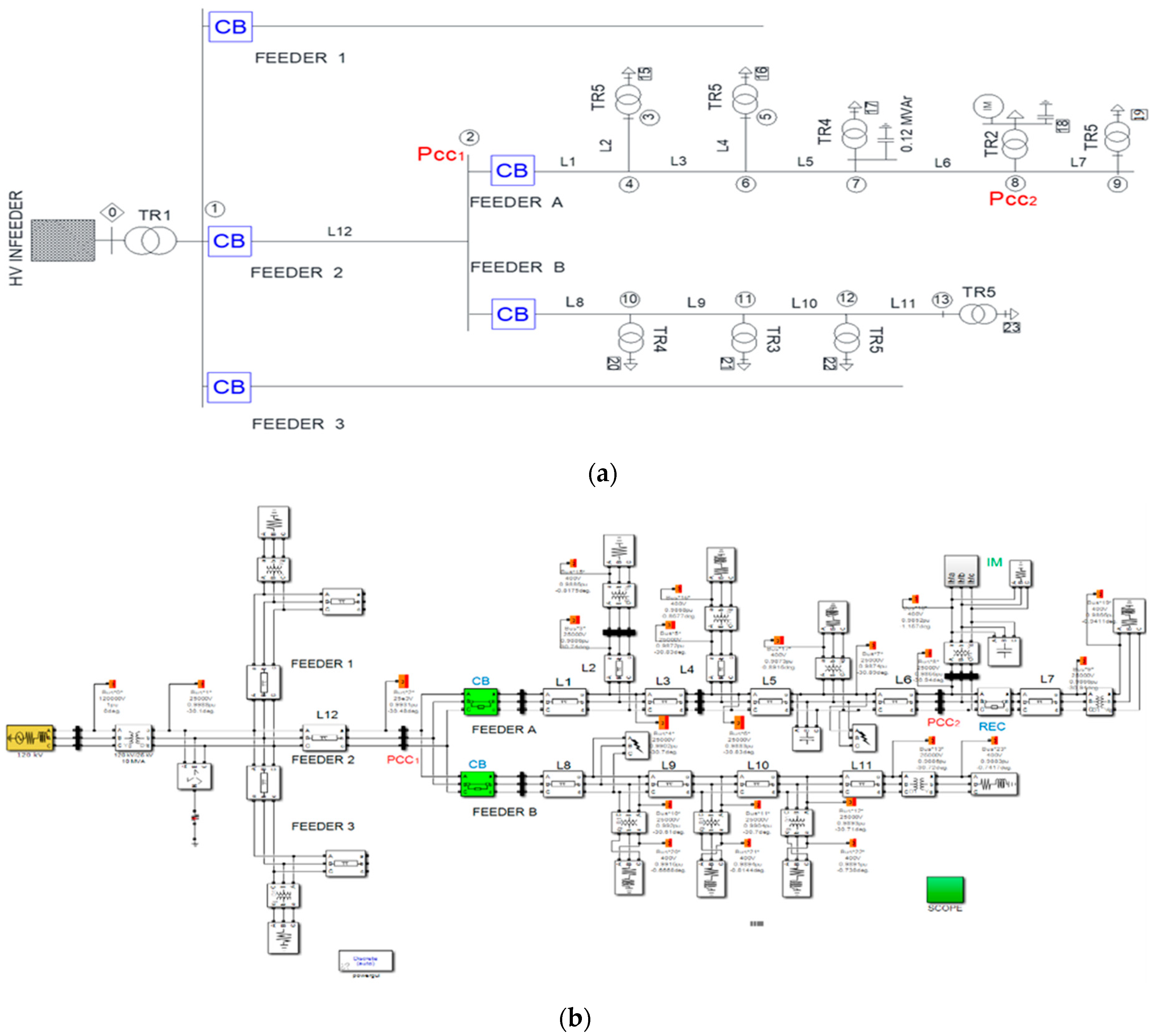
The system by which measurements have been recorded is a real DN which operates radially with an infeeder from a transmission system at 120 kV. The single-line diagram of the system is depicted in Figure 7a. As shown in the figure, the substation wye/delta transformer supplies three medium voltage (MV) feeders, Feeder 2 and Sub-Feeders A and B, forming the system analyzed in this work. It is relevant to point out that Feeders 1 and 3 are not detailed, because they are not relevant to the task due to their radial configuration and also because Feeder 1 is the faulted one in which the unintentional IO object of study occurs. The end-users are supplied at an LV of 0.4 kV through their MV/LV Dyn 11 transformers.
The MV system is grounded via a zig-zag transformer with a resistance of 23 Ω that limits the fault current to 630 A. The short circuit capacity at the 120 kV busbar is 1000 MVA. The main system parameters and the IMs data are detailed in Appendix A.
The equipment used to record the events comprise the protective relays installed at both PCC1 and PCC2. The fault recorder registers voltage and current signals with 32 samples per cycle. The overcurrent relays are equipped with an oscillography function; in PCC1, the relay registration is set to 400 ms, while in PCC2, this value is set to 600 ms. More information about the relays and their recording characteristics can be obtained from the manufacturer data available in Reference [65]. These relays record the voltage, currents, powers and frequency during the event. For each event, a pre-trigger of 200 ms is used in order to obtain the pre-fault active and reactive powers; thus, it is possible to compute the feeder-load power before the fault.
5. Simulation Results
This section will summarize the results of the simulations carried out in the three-phase Matlab/Simulink model adopted based on the single-line diagram of the real DN; see Figure 7b. The result discussion will be done by analysing the main features of the proposed voltage sag separately. Therefore, the further three subsections are as follows: (Section 5.1) gives the voltage sag magnitude, (Section 5.2) gives the voltage sag duration, and lastly (Section 5.3) gives the voltage recovery. The main parameters of the simulated scenarios are detailed in each subsection; nevertheless, the relay settings, fault characteristics and IM point of operation, which are the same for all simulations, are detailed below:
- An SLG fault with a fault resistance of 5 Ω is simulated at node 7; the implemented settings of the CB located at PCC1 (header of Feeder A, see Figure 7b) are listed in Table 1, where Iof represents an admissible overload factor; Ithreshold is the steady-state current threshold; and n, k, t are parameters of the curve. Particularly, the equation where the parameters mentioned above are used is defined in Equation (18). Besides, the most frequent curves for overcurrent protection are detailed in Reference [66]. The operation time T of the phase overcurrent relay is defined by Equation (18).where factor k is adjustable and typically ranges between 0.05 and 1.6, and n and t factors are used to choose the slope of the relay curves.
- IM is running under no-load torque at the time the fault occurs.
5.1. Voltage Sag Magnitude
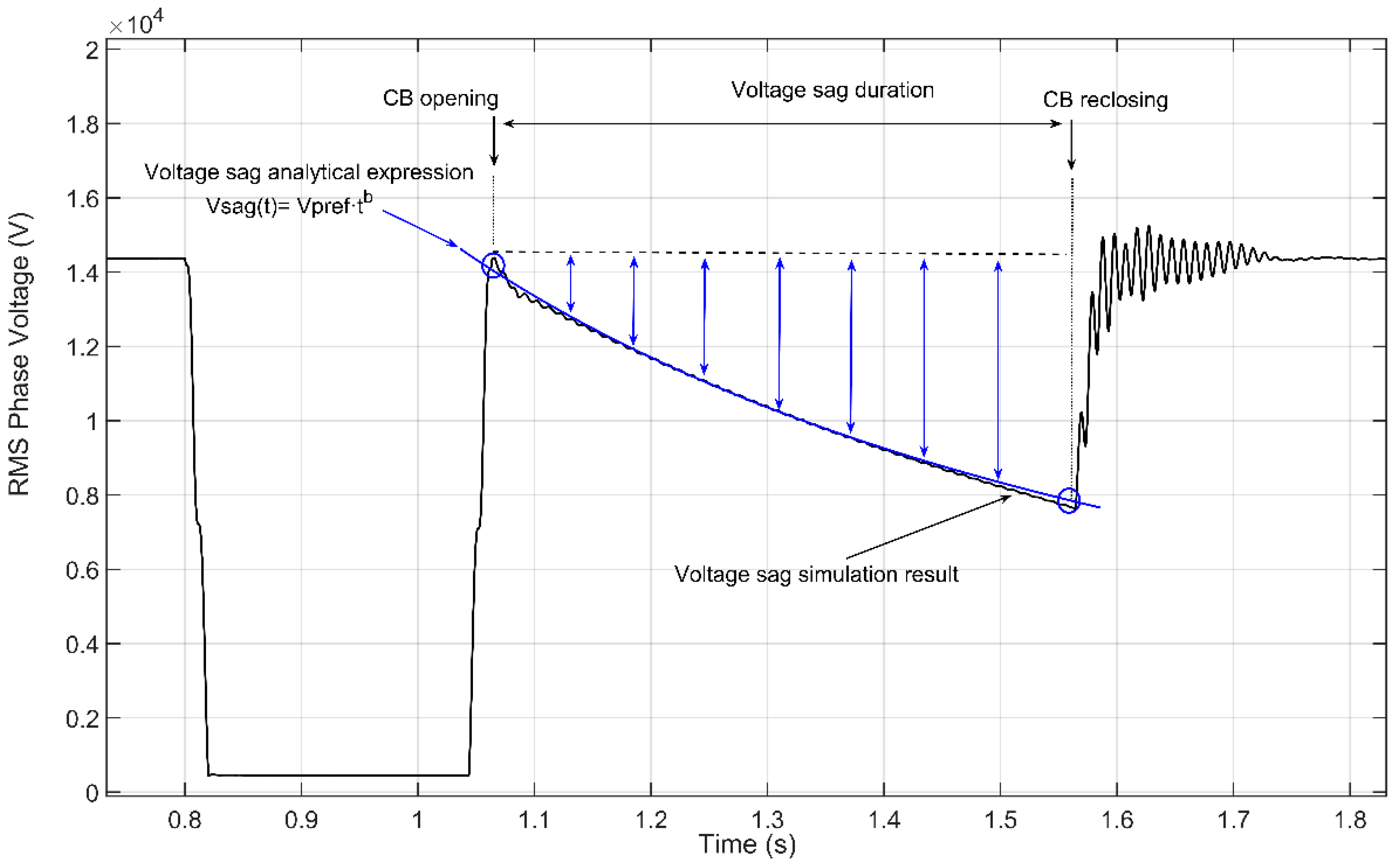
This part evaluates the simulation results with different values of feeder loads in order to analyze the different originated voltage sag characteristics and compare them with the previously described analytical expression. Figure 8 shows, as an example, one particular scenario and the analytical function that follows the voltage sag characteristic. In this simulation, the load feeders have been set to 53 kW. In the figure, the solid black line represents the simulation results, the solid blue line represents the analytical function of the voltage sag magnitude, and solid blue double arrows indicate the magnitude of the sag, which increases between ti (t = 1.05 s) and tf (t = 1.55 s).
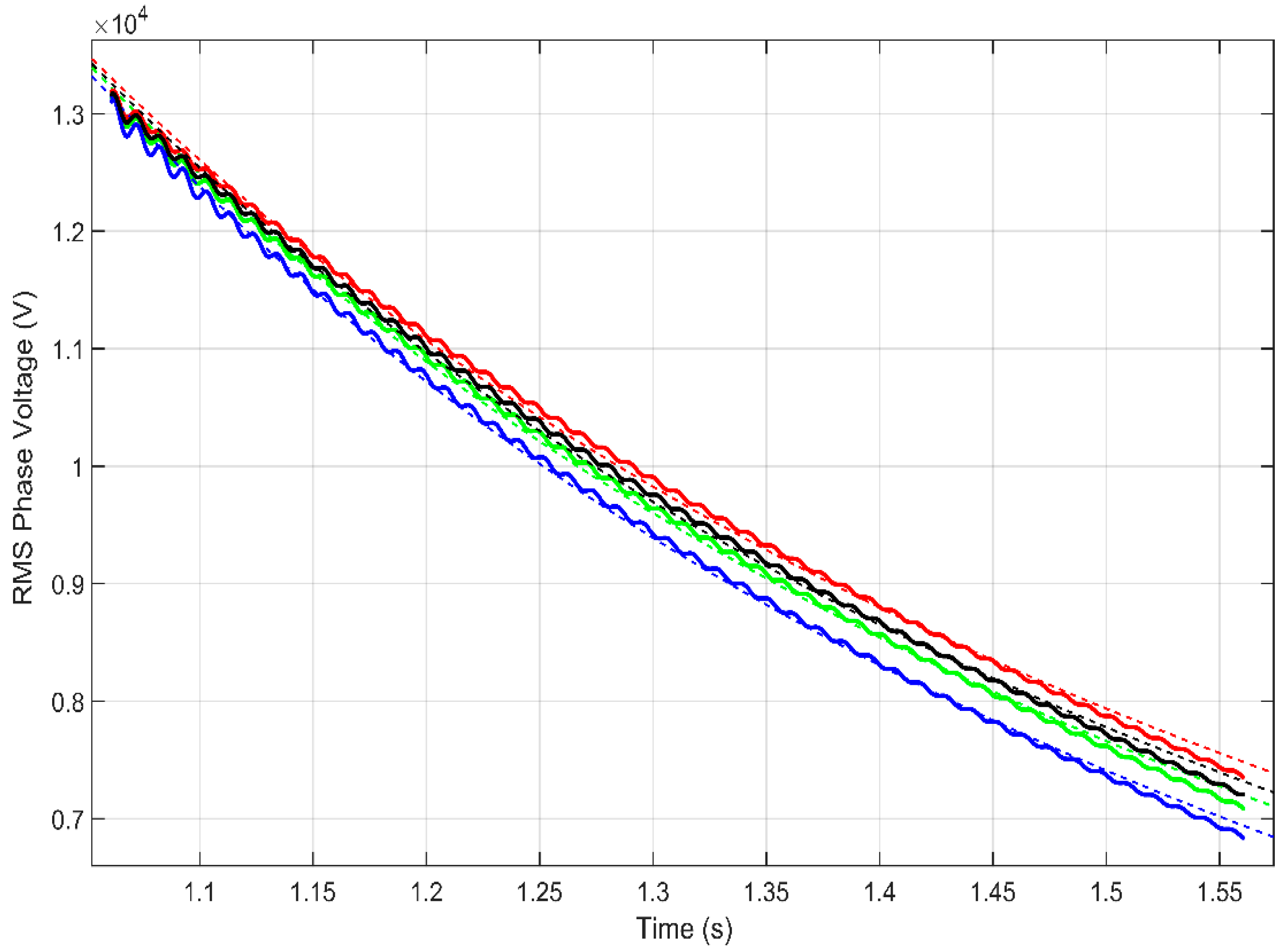
Moreover, four simulations have been performed with different feeder-load values in each one in order to observe different curve slopes. In Figure 9, four curves are displayed: the solid curves are the voltage magnitude of four voltage sags which result from simulations, and the dashed lines represent the function which fits the voltage sag magnitude according to each particular b value. Table 2 summarizes the main values of the simulated scenarios.
5.2. Voltage Sag Duration
In this section, four CB reclosing times have been tested to observe the duration of the voltage sag with a fixed value of feeder loads of 140 kW. From Figure 10, it can be seen that, depending on the reclosing time, as expected, the duration is higher, and consequently the voltage magnitude decreases with time. For all simulations, the initial time corresponds to 0.4 s when the CB clears the fault, and the sag recovery takes place depending on the reclosing time for each scenario.
5.3. Voltage Sag Recovery
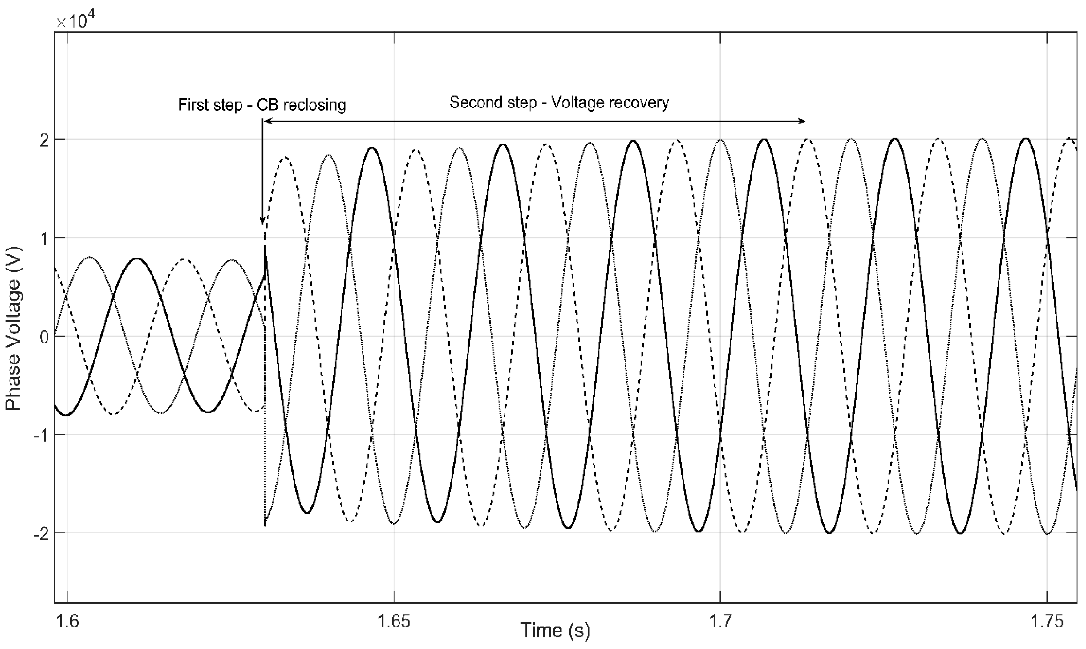
By observing Figure 11, as expected, the recovery takes place for all phases at the same instant, t = 1.63, when the CB recloses the circuit; however, the voltage amplitude is not recovered until 80 ms after this. Thereby, it has been demonstrated that defining the recovery process of this voltage sag accurately has to be done with two steps: the first is when the CB recloses the circuit, and the second is when the voltage reaches the pre-fault value.
6. Voltage Sag Model Validation
This section is focused on validating the proposed voltage sag, which has been analytically modelled in Section 3 by comparing simulation results with field measurements. For reasons of brevity, among all available real events, only two have been selected. Each event will be discussed separately detailing the voltage sag characteristics, and Table 3 summarizes the main features of these two events. Note that, since the voltage magnitude is non-constant, the voltage value of the fifth column of Table 3 is referred to the last RMS value before the reclosing takes place. Monitors have been installed at nodes PCC1 and PCC2 (See Figure 7a), and field measurements have been recorded at the highest voltage side of the MV/LV transformer in PCC2 where the IMs are allocated. In both Figure 12 and Figure 13, the three-phase voltages are compared, and simulation results are depicted in solid lines while field measurements are plotted in dashed lines.
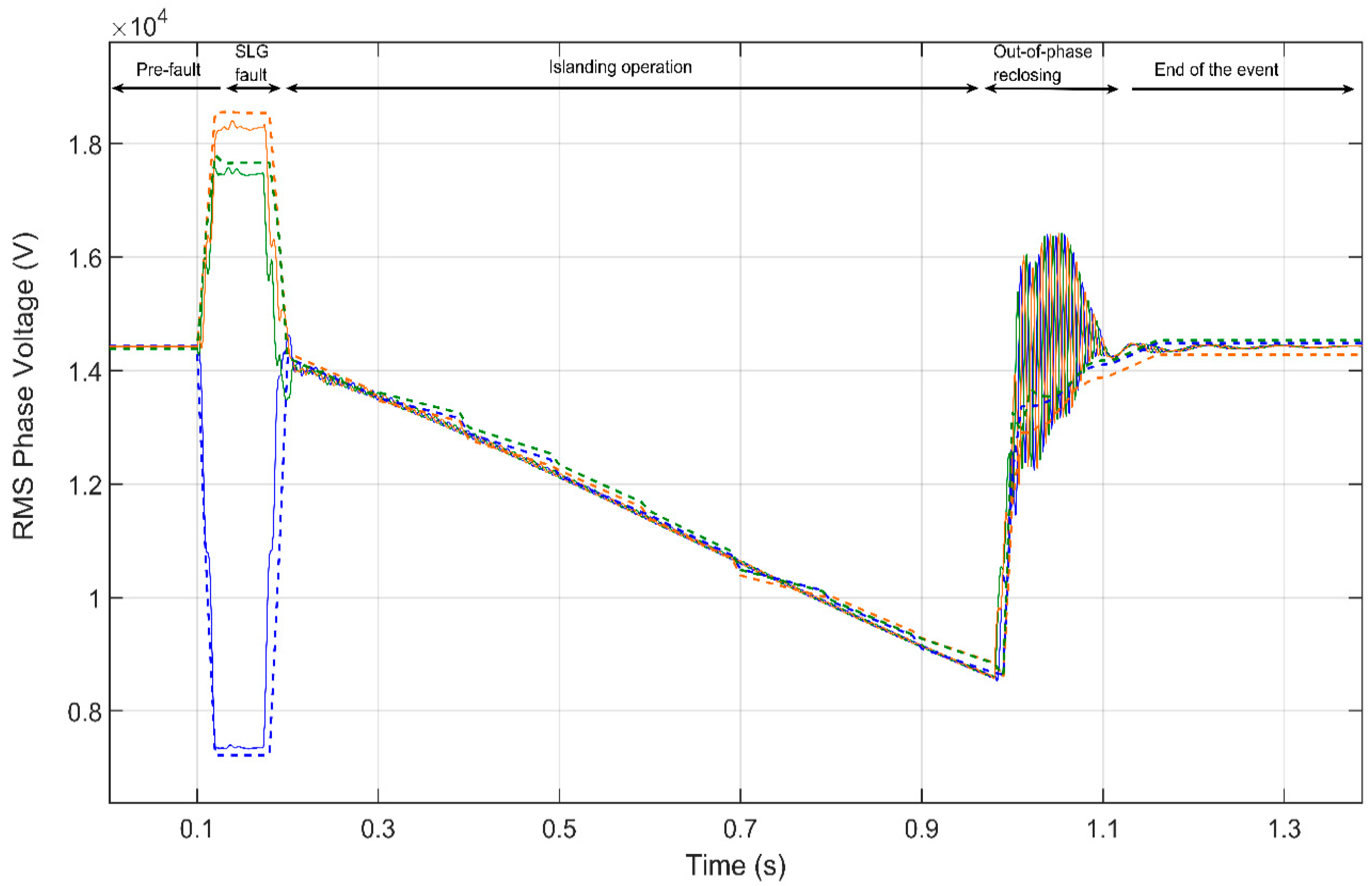
Event I: In Figure 12, the event starts in pre-fault conditions under a steady state until the SLG fault occurs at phase b in node 8 (See Figure 7a) at 0.1 s, and it is cleared within 100 ms. At that moment, the IMs were running under no-load torque, and the active-power value of the feeder loads was 810 kW. The voltage sag duration was 800 ms, coinciding with the CB reclosing time; at that time, the phase voltage was 8.78 kV for all phases in both simulation and field measurements. In this event, the voltage sag characteristic is defined by b = −1.05.
Event II: In Figure 13, the event starts in pre-fault conditions under a steady state until the SLG fault occurs at Phase C between Nodes 7 and 8 (Line 6) at 0.1 s, and it is cleared within 100 ms. At that moment, the IMs were running under no-load torque, and the active-power value of the feeder loads was 900 kW. The voltage sag duration was 800 ms, coinciding with the CB reclosing time; at that time, the phase voltage was 6 kV for all phases in both simulation and field measurements. In this event, the voltage sag characteristic is defined by b = −1.7. As in Event I, the recovery takes place in two stages: firstly, at the same instant for the three-phases due to the CB reclosing (t = 1 s), and the second step takes place at t = 1.12 s when the voltage is fully recovered.
It is essential to point out that after the first step of the recovery, between field measurements and simulations, a slight difference in the RMS phase voltage can be seen; this difference is due to the frequency dependence of the phase locked loop (PLL) measurement unit used in the simulation model and is also a result of the frequency oscillation during the recovery. Therefore, if the voltage waveform is taken into consideration instead of its computed RMS value, the simulation fits the recorded measurements equally for both events, and no oscillation appears. By observing the voltage of the waveform of Figure 11 in Section 5, one can observe that no oscillation occurs.
7. Conclusions
This paper makes a contribution to voltage sags characterization studies by presenting a novel voltage sag typology which occurs during unintentional IOs. Hence, the voltage sag has been analytically modelled, simulated and subsequently validated with field measurements recorded in a real DN.
As discussed in this paper, this voltage sag is defined as balanced, a non-constant retained voltage characterizes its magnitude, its duration is dictated by the CB reclosing, and its recovery takes place in a two-step process. One of the main goals of the present contribution is to describe the voltage sag non-constant voltage magnitude, which expands the present voltage sag typology. An analytical expression to model this voltage sag has been provided. It is seen that the voltage sag magnitude follows a negative exponential curve, and its slope is defined by b; this parameter is linked with the IM’s mechanical loss of speed. It has also been found that the higher the feeder loads value, the higher b is, and consequently, the higher the slope of the voltage sag is.
In Section 6, the voltage sag model validation has been carried out with two real events; the comparison between the simulations and these events undoubtedly underscore the appropriateness of the presented analytical expression, as well as evidencing the accuracy of the three-phase Matlab/Simulink model adopted.
Further work will be focused on the equipment sensitivity analysis for this particular voltage sag via hardware-in-the-loop testing.
Author Contributions
All the authors have contributed equally to this study.
Funding
This research was funded by the Catalonian College of engineers, grant number EICPhD-2018.
Acknowledgments
The authors want to acknowledge the financial support and the willingness of sharing field measurements by the Spanish DSO Electrica Serosense Distribuidora. The authors would also like to thank the Catalonian College of Engineers for the grant received to carry out this research.
Conflicts of Interest
The authors declare no conflicts of interest.
Appendix A

Table A1.
Test system parameters.
| Transformers | |||||||
| Vp/Vs (kV) | S (MVA) | ε (%) | Lm/Rm (H/kΩ) | ||||
| Substation transformer | TR1 | 120/25 kV | 10 | 10.4 | 78; 313 | ||
| Distribution transformers | TR2 | 25/0.4 kV | 1 | 6 | 180; 370 | ||
| TR3 | 25/0.4 kV | 0.63 | 5.1 | 350; 480 | |||
| TR4 | 25/0.4 kV | 0.4 | 4.3 | 404; 694 | |||
| TR5 | 25/0.4 kV | 0.25 | 4.1 | 811; 1666 | |||
| Distribution Lines | |||||||
| Lines | Nodes | Length (km) | Parameters: Z1/Z0 (Ω/km); C0 (μF/km) | Loadability (A) | |||
| L1 | 2–4 | 5 | 0.306+j0.405/0.38+j1.62 | 300 | |||
| L2 | 4–3 | 3.3 | 1.07+j0.441/1.3+j1.76, | 120 | |||
| L3 | 4–6 | 4.3 | 0.306+j0.405/0.38+j1.62 | 300 | |||
| L4 | 6–5 | 4 | 1.07+j0.441/1.3+j1.76 | 120 | |||
| L5 | 6–7 | 2.5 | 0.306+j0.405/0.38+j1.62 | 300 | |||
| L6 | 7–8 | 2 | 0.306+j0.405/0.38+j1.62 | 300 | |||
| L7 | 8–9 | 7 | 0.687+j0.416/0.8+j1.66 | 200 | |||
| L8 | 2–10 | 3.8 | 0.127+j0.114/0.17+j0.45; 0.229 | 389 | |||
| L9 | 10–11 | 4.43 | 0.208+j0.123/0.278+j0.492; 0.192 | 320 | |||
| L10 | 11–12 | 4 | 0.687+j0.416/0.8+j1.66 | 200 | |||
| L11 | 12–13 | 3.3 | 0.687+j0.416/0.8+j1.66 | 200 | |||
| L12 | 1–2 | 0.28 | 0.306+j0.405/0.38+j1.62 | 300 | |||
Table A2.
Induction motor (IM) data.
| Internal Parameters | Values | Rated Parameters | Values |
|---|---|---|---|
| Ls | 0.0078 H | P | 160 kW |
| Lr | 0.0078 H | 𝓅 | 1 |
| Rr | 0.0077 Ω | f | 50 Hz |
| Rs | 0.0137 Ω | V | 400 V |
| Lm | 0.0076 H | J | 2.9 kgm2 |
References
- Moreno-Munõoz, A.; González de la Rosa, J.J. Integrating power quality to automated meter reading. IEEE Ind. Electron. Mag. 2008, 2, 10–18. [Google Scholar] [CrossRef]
- Ali, S.; Wu, K.; Weston, K.; Marinakis, D. A machine learning approach to meter placement for Power Quality Estimation in Smart Grid. IEEE Trans. Smart Grid 2016, 7, 1552–1561. [Google Scholar] [CrossRef]
- Broshi, A. Monitoring Power Quality Beyond EN 50160 and IEC 61000-4-30. In Proceedings of the 2007 9th International Conference on Electrical Power Quality and Utilisation, EPQU, Barcelona, Spain, 9–11 October 2007. [Google Scholar]
- Gosbell, V.J.; Baitch, A.; Bollen, M.H. The Reporting of Distribution Power Quality Surveys. In Proceedings of the CIGRE/IEEE PES International Symposium Quality and Security of Electric Power Delivery Systems, CIGRE/PES 2003, Montreal, QC, Canada, 8–10 October 2003; pp. 48–52. [Google Scholar]
- Florencias-Oliveros, O.; Agüera-Pérez, A.; González-De-La-Rosa, J.-J.; Palomares-Salas, J.-C.; Sierra-Fernández-Álvaro, J.-M.; Montero, J. Cluster Analysis for Power Quality Monitoring. Qualitative Analysis Based in Higher-Order Statistics for the Smart Grid. In Proceedings of the 2017 11th IEEE International Conference on Compatibility, Power Electronics and Power Engineering (CPE-POWERENG), Cadiz, Spain, 4–6 April 2017. [Google Scholar]
- Mei, F.; Ren, Y.; Wu, Q.; Zhang, C.; Pan, Y.; Sha, H.; Zheng, J. Online Recognition Method for Voltage sags based on a deep belief network. Energies 2018, 12, 43. [Google Scholar] [CrossRef]
- Guerrero-Rodríguez, J.M.; Cobos-Sánchez, C.; González-de-la-Rosa, J.J.; Sales-Lérida, D. An Embedded Sensor Node for the Surveillance of. Energies 2019, 12, 1561. [Google Scholar] [CrossRef]
- de la Rosa, J.J.; Muñoz, A.M.; de Castro, A.G.; López, V.P.; Sánchez Castillejo, J.A. A web-based distributed measurement system for electrical power quality assessment. Meas. J. Int. Meas. Confed. 2010, 43, 771–780. [Google Scholar] [CrossRef]
- Cisneros-Maga, R.A.; Medina, A.; Anaya-Lara, O. Time-domain voltage sag state estimation based on the unscented kalman filter for power systems with nonlinear components. Energies 2018, 11, 1411. [Google Scholar] [CrossRef]
- Otcenasova, A.; Bodnar, R.; Regula, M.; Hoger, M.; Repak, M. Methodology for determination of the number of equipment malfunctions due to voltage sags. Energies 2017, 10, 401. [Google Scholar] [CrossRef]
- Bollen, M.H.; Styvaktakis, E.; Gu, I.Y. Categorization and analysis of power system transients. IEEE Trans. Power Deliv. 2005, 20, 2298–2306. [Google Scholar] [CrossRef]
- de la Rosa, J.; Sierra-Fernández, J.; Palomares-Salas, J.; Agüera-Pérez, A.; Montero, Á. An application of spectral kurtosis to separate hybrid power quality events. Energies 2015, 8, 9777–9793. [Google Scholar] [CrossRef]
- Florencias-Oliveros, O.; González-de-la-Rosa, J.J.; Agüera-Pérez, A.; Palomares-Salas, J.C. Reliability monitoring based on higher-order statistics: A scalable proposal for the smart grid. Energies 2019, 12, 55. [Google Scholar] [CrossRef]
- Shen, Y.; Abubakar, M.; Liu, H.; Hussain, F. Power Quality Disturbance Monitoring and Classification Based on Improved PCA and Convolution Neural Network for Wind-Grid Distribution Systems. Energies 2019, 12, 1280. [Google Scholar] [CrossRef]
- Saini, M.K.; Kapoor, R. Classification of power quality events—A review. Int. J. Electr. Power Energy Syst. 2012, 43, 11–19. [Google Scholar] [CrossRef]
- Reaz, M.B.; Choong, F.; Sulaiman, M.S.; Mohd-Yasin, F.; Kamada, M. Expert system for power quality disturbance classifier. IEEE Trans. Power Deliv. 2007, 22, 1979–1988. [Google Scholar] [CrossRef]
- Youssef, A.M.; Abdel-Galil, T.K.; El-Saadany, E.F.; Salama, M.M.A. Disturbance Classification Utilizing Dynamic Time Warping Classifier. IEEE Trans. Power Deliv. 2004, 19, 272–278. [Google Scholar] [CrossRef]
- Valtierra-Rodriguez, M.; De Jesus Romero-Troncoso, R.; Osornio-Rios, R.A.; Garcia-Perez, A. Detection and classification of single and combined power quality disturbances using neural networks. IEEE Trans. Ind. Electron. 2014, 61, 2473–2482. [Google Scholar] [CrossRef]
- Huang, C.H.; Lin, C.H.; Kuo, C.L. Chaos synchronization-based detector for power-quality disturbances classification in a power system. IEEE Trans. Power Deliv. 2011, 26, 944–953. [Google Scholar] [CrossRef]
- Manikandan, M.S.; Samantaray, S.R.; Kamwa, I. Detection and classification of power quality disturbances using sparse signal decomposition on hybrid dictionaries. IEEE Trans. Instrum. Meas. 2015, 64, 27–38. [Google Scholar] [CrossRef]
- Massignan, J.A.; London, J.B.; Bessani, M.; Maciel, C.D.; Delbem, A.C.; Camillo, M.H.; de Lima Soares, T.W. In-field Validation of a Real Time Monitoring tool for distribution feeders. IEEE Trans. Power Deliv. 2017, 33, 1798–1808. [Google Scholar] [CrossRef]
- Cai, L.; Thornhill, N.F.; Kuenzel, S.; Pal, B.C. Real-Time Detection of Power System Disturbances Based on k-Nearest Neighbor Analysis. IEEE Access 2017, 5, 5631–5639. [Google Scholar] [CrossRef]
- Perez, E.; Barros, J. A proposal for on-line detection and classification of voltage events in power systems. IEEE Trans. Power Deliv. 2008, 23, 2132–2138. [Google Scholar] [CrossRef]
- Borghetti, A.; Bosetti, M.; Nucci, C.A.; Paolone, M.; Abur, A. Integrated use of time-frequency wavelet decompositions for fault location in distribution networks: Theory and experimental validation. IEEE Trans. Power Deliv. 2010, 25, 3139–3146. [Google Scholar] [CrossRef]
- Faried, S.O.; Member, S.; Aboreshaid, S.; Member, S. Stochastic Evaluation of Voltage Sags in Series Capacitor Compensated Radial Distribution Systems. IEEE Trans. Power Deliv. 2003, 18, 744–750. [Google Scholar] [CrossRef]
- Quality, E.P. Stochastic Estimation of Voltage Sag Due to Faults in the Power System by Using PSCAD/EMTDC Software as a Tool for Simulation. Power Qual. 2007, 13, 59–63. [Google Scholar]
- Martínez-Velasco, J.A. Computer-based voltage Dip Assessment in transmission and distribution networks. Electr. Power Qual. Util. J. 2008, 14, 31–38. [Google Scholar]
- Martinez-Velasco, J.A.; Martin-Arnedo, J. Voltage sag studies in distribution networks—Part I: System modeling. IEEE Trans. Power Deliv. 2006, 21, 1670–1678. [Google Scholar] [CrossRef]
- Martinez-Velasco, J.A.; Martin-arnedo, J. Voltage Sag Studies in Distribution Networks—Part II: Voltage Sag Assessment. IEEE Trans. Power Deliv. 2006, 21, 1679–1688. [Google Scholar] [CrossRef]
- Martinez-Velasco, J.A.; Martin-arnedo, J. EMTP model for analysis of distributed generation impact on voltage sags. IET Gener. Transm. Distrib. 2007, 1, 112–119. [Google Scholar]
- Bollen, M.H.J.; Bahramirad, S.; Khodaei, A. Is There a Place for Power Quality in the Smart Grid? In Proceedings of the International Conference on Harmonics and Quality of Power, ICHQP, Bucharest, Romania, 25–28 May 2014. [Google Scholar]
- Bollen, M.H.J.; Olguin, G.; Martins, M. Voltage dips at the terminals of wind power installations. Wind Energy 2005, 8, 307–318. [Google Scholar] [CrossRef]
- Sabin, D.D.; Bollen, M.H. Overview of IEEE Std 1564-2014 Guide for Voltage Sag Indices. In Proceedings of the International Conference on Harmonics and Quality of Power, ICHQP, Bucharest, Romania, 25–28 May 2014. [Google Scholar]
- Dash, P.K.; Padhee, M.; Barik, S.K. Estimation of power quality indices in distributed generation systems during power islanding conditions. Int. J. Electr. Power Energy Syst. 2012, 36, 18–30. [Google Scholar] [CrossRef]
- Martinez-Velasco, J.A.; Martin-Arnedo, J. Voltage Sag Studies in Distribution Networks—Part III: Voltage Sag Index Calculation. IEEE Trans. Power Deliv. 2006, 21, 1689–1697. [Google Scholar] [CrossRef]
- Otcenasova, A.; Bolf, A.; Altus, J.; Regula, M. The Influence of Power Quality Indices on Active Power Losses in a Local Distribution Grid. Energies 2019, 12, 1389. [Google Scholar] [CrossRef]
- Golovanov, N.; Lazaroiu, G.C.; Roscia, M.; Zaninelli, D. Power quality assessment in small scale renewable energy sources supplying distribution systems. Energies 2013, 6, 634–645. [Google Scholar] [CrossRef]
- Markiewicz, H.; Klajn, A. EN 50160—Voltage Characteristics in Public Distribution Systems. Cenelec, 1 July 2001. Available online: https://standards.globalspec.com/std/9943573/EN2050160 (accessed on 9 July 2019).
- Bollen, M.H. Understanding Power Quality Problems; IEEE press: Piscataway, NJ, USA, 2000. [Google Scholar]
- Bollen, M.H.; Gu, I.Y. Signal Processing of Power Quality Disturbances; John Wiley & Sons: Hoboken, NJ, USA, 2005. [Google Scholar]
- Rönnberg, S.; Bollen, M. Power quality issues in the electric power system of the future. Electr. J. 2016, 29, 49–61. [Google Scholar] [CrossRef]
- Yalçinkaya, G. Characterization of voltage sags in industrial distribution systems. IEEE Trans. Ind. Appl. 1998, 34, 682–688. [Google Scholar] [CrossRef]
- CIGRE/CIRED/UIE Joint Working Group C4.110. Voltage Dip Immunity of Equipment and Installations. CIGRE. Publ., 2010; pp. 1–18. Available online: http://www.uie.org/sites/default/files/CIGRE%20TB412%20voltage%20dip%20immunity%20of%20equipment%20and%20installations.pdf (accessed on 9 July 2019).
- Bollen, M.H.; Cundeva, S.; Gordon, J.M.; Djokic, S.Z.; Stockman, K.; Milanovic, J.V.; Neumann, R.; Ethier, G. Voltage dip immunity aspects of power-electronics equipment—Recommendations from CIGRE/CIRED/UIE JWG C4.110. Proceeding of the International Conference on Electrical Power Quality and Utilisation, EPQU, Ohrid, Macedonia, 6–8 September 2011. [Google Scholar]
- Pedra, J.; Bogarra, S.; Córcoles, F.; Monjo, L.; Rolán, A. Testing of three-phase equipment under voltage sags. IET Electr. Power Appl. 2015, 9, 287–296. [Google Scholar]
- Bollen, M.H. Characterisation of voltage sags experienced by three-phase adjustable-speed drives. IEEE Trans. Power Deliv. 1997, 12, 1666–1671. [Google Scholar] [CrossRef]
- Milanović, J.V.; Gupta, C.P. Probabilistic assessment of financial losses due to interruptions and voltage sags—Part II: Practical implementation. IEEE Trans. Power Deliv. 2006, 21, 925–932. [Google Scholar] [CrossRef]
- Dolara, A.; Leva, S. Power quality and harmonic analysis of end user devices. Energies 2012, 5, 5453–5466. [Google Scholar] [CrossRef]
- Yang, Y.; Xiao, X.; Guo, S.; Gao, Y.; Yuan, C.; Yang, W. Energy storage characteristic analysis of voltage sags compensation for UPQC based on MMC for medium voltage distribution system. Energies 2018, 11, 923. [Google Scholar] [CrossRef]
- Tien, D.; Gono, R.; Leonowicz, Z. A multifunctional dynamic voltage restorer for power quality improvement. Energies 2018, 11, 1351. [Google Scholar] [CrossRef]
- Roncero-Sánchez, P.; Acha, E. Design of a control scheme for distribution static synchronous compensators with power-quality improvement capability. Energies 2014, 7, 2476–2497. [Google Scholar] [CrossRef]
- Beckwith, T.R.; Hartmann, W.G. Motor bus transfer: Considerations and methods. IEEE Trans. Ind. Appl. 2006, 42, 602–611. [Google Scholar] [CrossRef]
- Muralimanohar, P.K.; Haas, D.; McClanahan, J.R.; Jagaduri, R.T.; Singletary, S. Implementation of a Microprocessor-Based Motor Bus Transfer Scheme. IEEE Trans. Ind. Appl. 2018, 54, 4001–4008. [Google Scholar] [CrossRef]
- Varadarajan, M.; Swarup, K.S. Advanced Voltage Sag Characteristics: Point on Wave. Gener. Transm. Distrib. IET 2007, 1, 324. [Google Scholar]
- Bastos, A.F.; Lao, K.W.; Todeschini, G.; Santoso, S. Accurate Identification of Point-on-Wave Inception and Recovery Instants of Voltage Sags and Swells. IEEE Trans. Power Deliv. 2019, 34, 551–560. [Google Scholar] [CrossRef]
- Wang, Y.; Bagheri, A.; Bollen, M.H.; Xiao, X.Y. Single-Event Characteristics for Voltage Dips in Three-Phase Systems. IEEE Trans. Power Deliv. 2017, 32, 832–840. [Google Scholar] [CrossRef]
- Madrigal, M.; Rocha, B.H. A contribution for characterizing measured three-phase unbalanced voltage sags algorithm. IEEE Trans. Power Deliv. 2007, 22, 1885–1890. [Google Scholar] [CrossRef]
- Bollen, M.H. Algorithms for characterizing measured three-phase unbalanced voltage dips. IEEE Trans. Power Deliv. 2003, 18, 937–944. [Google Scholar] [CrossRef]
- Cai, D.; Li, K.; He, S.; Li, Y.; Luo, Y. On the application of joint-domain dictionary mapping for multiple power disturbance assessment. Energies 2018, 11, 347. [Google Scholar] [CrossRef]
- Zhang, L.; Bollen, M.H. Method for Characterisation of Three-Phase Unbalanced Dips (Sags) from Recorded Voltage Waveshapes. In Proceedings of the 21st International Telecommunications Energy Conference, INTELEC’99 (Cat. No. 99CH37007), Copenhagen, Denmark, 9 June 1999; p. 188. [Google Scholar]
- Bollen, M.H.; Styvaktakis, E. Characterization of Three-Phase Unbalanced Dips (as Easy as One-Two-Three?). In Proceedings of the International Conference on Harmonics and Quality of Power, ICHQP, Orlando, FL, USA, 1–4 October 2000; Volume 1, pp. 81–86. [Google Scholar]
- Bollen, M.H. Influence of motor reacceleration on voltage sags. IEEE Trans. Ind. Appl. 1995, 31, 667–674. [Google Scholar] [CrossRef]
- IEEE Power Engineering Society; IEEE Power Electronics Society; IEEE Industry Applications Society; Bollen, M.H. Understanding Power Quality Problems: Voltage Sags and Interruptions; IEEE Press: Piscataway, NJ, USA, 2000. [Google Scholar]
- Martinez, J.A.; Walling, R.; Mork, B.A.; Martin-Arnedo, J.; Durbak, D. Parameter determination for modeling system transients-Part III: Transformers. IEEE Trans. Power Deliv. 2005, 20, 2051–2062. [Google Scholar] [CrossRef]
- Ormazabal Protection and Automation. EkorRPS-Multifunctional Protection. Available online: https://www.ormazabal.com/es/tu-negocio/productos/ekorrps (accessed on 9 July 2019).
- Benmouyal, G.; Meisinger, M.; Burnworth, J.; Elmore, W.A.; Freirich, K.; Kotos, P.A.; Leblanc, P.R.; Lerley, P.J.; McConnell, J.E.; Mizener, J.; et al. IEEE standard inverse-time characteristic equations for overcurrent relays. IEEE Trans. Power Deliv. 1999, 14, 868–871. [Google Scholar] [CrossRef]
Figure 1.
Example of a constant voltage sag produced by a single-line-to-ground (SLG) fault and its characteristics.
Figure 1.
Example of a constant voltage sag produced by a single-line-to-ground (SLG) fault and its characteristics.

Figure 2.
Example of a non-constant voltage sag produced by an induction motor (IM) start.

Figure 3.
Example of a non-constant voltage sag produced for a three-phase fault with IMs. (a) RMS voltage and current during the event; (b) enlarged section of the voltage sag characteristic.
Figure 3.
Example of a non-constant voltage sag produced for a three-phase fault with IMs. (a) RMS voltage and current during the event; (b) enlarged section of the voltage sag characteristic.

Figure 4.
Example of a non-constant voltage sag produced by transformer energization.

Figure 5.
Comparison between scenarios, distribution network (DN) with IMs (solid line) and without IMs (dashed line).
Figure 5.
Comparison between scenarios, distribution network (DN) with IMs (solid line) and without IMs (dashed line).

Figure 6.
Voltage sag analytical function for a given b parameter.

Figure 7.
Test system under study. (a) One-line diagram of the test system.; (b) Matlab/Simulink implementation of the test system.
Figure 7.
Test system under study. (a) One-line diagram of the test system.; (b) Matlab/Simulink implementation of the test system.

Figure 8.
Voltage sag magnitude comparison between simulation results and the proposed analytical curve.
Figure 8.
Voltage sag magnitude comparison between simulation results and the proposed analytical curve.

Figure 9.
Voltage sag magnitude of the four simulated scenarios with different feeder-load values.

Figure 10.
Voltage sag duration for the four simulated reclosing times.

Figure 11.
Two-step voltage sag recovery.

Figure 12.
Event I comparison. Solid (simulation)/dashed (measurements): orange (Phase A), blue (Phase B) and green (Phase C).
Figure 12.
Event I comparison. Solid (simulation)/dashed (measurements): orange (Phase A), blue (Phase B) and green (Phase C).

Figure 13.
Event II comparison. Solid (simulation)/dashed (measurements): orange (Phase A), blue (Phase B) and green (Phase C).
Figure 13.
Event II comparison. Solid (simulation)/dashed (measurements): orange (Phase A), blue (Phase B) and green (Phase C).
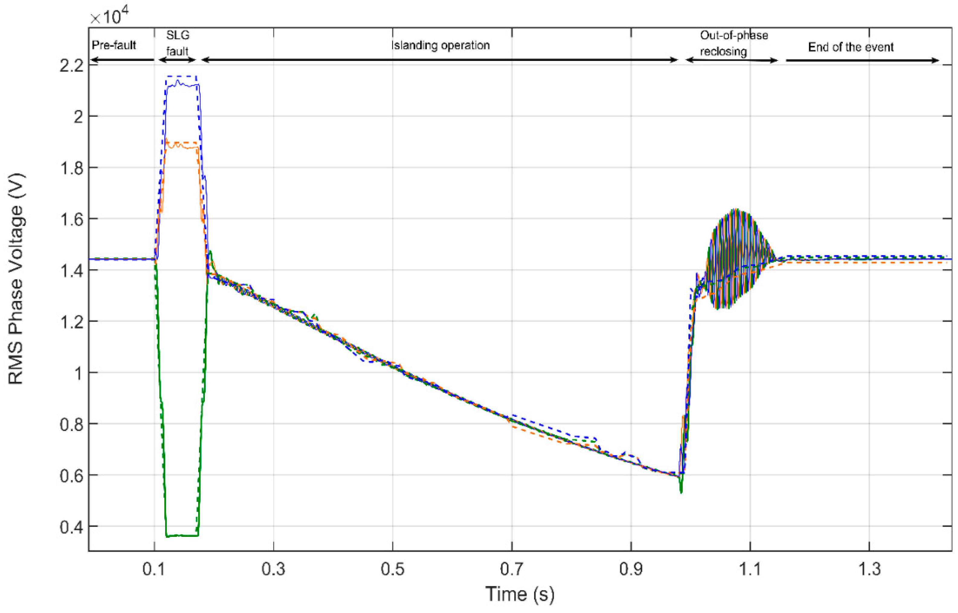
Table 1.
Overcurrent relay parameters.
| ANSI Code | k | n | t | Ithreshold (A) | Iof | ANSI Curve |
|---|---|---|---|---|---|---|
| 50 | 0.05 | 0.02 | 0.14 | 100 | 1.25 | Standard inverse |
Table 2.
Simulated scenarios and resulting parameters of Section 5.1.
Table 2.
Simulated scenarios and resulting parameters of Section 5.1.
| Scenarios | Color | Feeder Loads (kW) | b | ΔV (pu) | Duration (ms) |
|---|---|---|---|---|---|
| 1 | Red | 64 | −1.492 | 0.49 | 500 |
| 2 | Black | 80 | −1.54 | 0.5 | 500 |
| 3 | Green | 100 | −1.576 | 0.51 | 500 |
| 4 | Blue | 128 | −1.655 | 0.53 | 500 |
Table 3.
Voltage sags characteristic summary for Events I and II.
| Event | Beginning (h) | Ending (h) | b | Sag Magnitude (pu) | Sag Duration (ms) |
|---|---|---|---|---|---|
| I | 17:01:09.776 | 17:01:10.636 | −1.05 | 0.61 | 800 |
| II | 11:49:04.702 | 11:49:05.456 | −1.7 | 0.41 | 800 |
© 2019 by the authors. Licensee MDPI, Basel, Switzerland. This article is an open access article distributed under the terms and conditions of the Creative Commons Attribution (CC BY) license (http://creativecommons.org/licenses/by/4.0/).
Share and Cite
MDPI and ACS Style
Serrano-Fontova, A.; Casals Torrens, P.; Bosch, R. Power Quality Disturbances Assessment during Unintentional Islanding Scenarios. A Contribution to Voltage Sag Studies. Energies 2019, 12, 3198. https://doi.org/10.3390/en12163198
AMA Style
Serrano-Fontova A, Casals Torrens P, Bosch R. Power Quality Disturbances Assessment during Unintentional Islanding Scenarios. A Contribution to Voltage Sag Studies. Energies. 2019; 12(16):3198. https://doi.org/10.3390/en12163198
Chicago/Turabian StyleSerrano-Fontova, Alexandre, Pablo Casals Torrens, and Ricard Bosch. 2019. "Power Quality Disturbances Assessment during Unintentional Islanding Scenarios. A Contribution to Voltage Sag Studies" Energies 12, no. 16: 3198. https://doi.org/10.3390/en12163198
Note that from the first issue of 2016, this journal uses article numbers instead of page numbers. See further details here.