Probabilistic Power Flow for Hybrid AC/DC Grids with Ninth-Order Polynomial Normal Transformation and Inherited Latin Hypercube Sampling

Abstract

This paper proposes a new probabilistic power flow method for the hybrid AC/VSC-MTDC (Voltage Source Control-Multiple Terminal Direct Current) grids, which is based on the combination of ninth-order polynomial normal transformation (NPNT) and inherited Latin hypercube sampling (ILHS) techniques. NPNT is utilized to directly handle historical records of uncertain sources to build the accurate probability model of random inputs, and ILHS is adopted to propagate the randomness from inputs to target outputs. Regardless of whether the underlying probability distribution is known or unknown, the proposed method has the ability to adaptively evaluate the sample size according to a specific operational scenario of the power systems, thus achieving a good balance between computational accuracy and speed. Meanwhile, the frequency histograms, probability distributions, and some more statistics of the results can be accurately and efficiently estimated as well. The modified IEEE 118-bus system, together with the realistic data of wind speeds and diverse consumer behaviors following irregular distributions, is used to demonstrate the effectiveness and superiority of the proposed method.

1. Introduction

The Voltage Source Converter based Multiple Terminal Direct Current (VSC-MTDC) technique has become the most feasible solution to the integration of remotely located large wind farms (WFs), as it can effectively support the AC grid, facilitate the integration of fluctuant wind power, and improve the transfer efficiency [1]. With more and more WFs integrated into AC grids by using VSC-MTDC, the fluctuant wind power will significantly increase the stochastic nature of the power system, thus further exacerbating the operational condition of the hybrid AC/VSC-MTDC grids [2]. Nevertheless, the deterministic power flow (DPF) cannot fully account for the random variables. Hence, the probabilistic power flow (PPF) methods for the hybrid AC/VSC-MTDC grid are rising with the aim of accurately evaluating the impact of probabilistic uncertainties.

In power system operation, the PPF analysis treats the uncertainties (such as wind speeds and loads) as input variables, and it focuses on accurately obtaining the statistical information of outputs including mean, standard deviation, frequency histogram, and even probability density function (PDF) based on the results within an acceptable computational time. To achieve this goal, the following problems are necessary to be considered and addressed:

(1)

the probability model of input variables needs to be accurately built based on the historical records, regardless of whether the underlying distribution is known or unknown;

(2)

the probabilistic method holds a good balance between computation accuracy and speed;

(3)

the mean, standard deviation, frequency histogram, and even the PDF of output results obtained from PPF calculation can be comprehensively available.

The first problem is the issue of handling random input variables. With the construction of a VSC-MTDC system, the power grid will constantly expand, and massive uncertain sources will emerge [3]. These uncertain sources in a hybrid AC/VSC-MTDC grid may follow arbitrary distributions since they are distributed in a wide geographic space and affected by various complex factors e.g., meteorological conditions. Meanwhile, the correlation amongst these random variables of adjacent areas cannot be neglected. Hence, the established probability model of input variables in the hybrid AC/VSC-MTDC grid should have the ability to consider correlated random variables following diverse even irregular distributions. However, the uncertain sources in PPF calculation were assumed to follow some common probability distributions. Under such assumption, the loads were subject to Gaussian distributions in [4,5,6]; and, the wind speeds were set to follow Weibull distributions in [7,8,9]. Subsequently, based on the selected common distributions with their analytical expressions, the NATAF transformation can be applied to establish the correlation relationship amongst random input variables [7,8,10]. In a few cases, the established probability model according to assumption makes sense. Unfortunately, the loads and wind speeds in a practical hybrid AC/VSC-MTDC grid may not follow common distributions but irregular distributions. Based on the assumption of input variables following common distributions, the approximated probability model will bring significant error, resulting in an accuracy loss.

The polynomial normal transformation technique is not only able to handle the random variables following irregular distributions but also has the ability to deal with the correlations among these variables. In [11], the third-order polynomial normal transformation (TPNT) is introduced into the PPF analysis for pure AC grid to directly deal with historical records of wind speeds and loads. To improve the accuracy in the approximations of some irregular distributions, Headrick proposes the fifth-order polynomial normal transformation (FPNT) [12]. However, these two techniques are still limited to a portion of distribution types and hence are unable to accurately model some distributions of wind speeds and loads that follow irregular or extremely uncommon distributions in practice. In this paper, a ninth-order polynomial normal transformation (NPNT) technique [13,14] is firstly employed to model the random variables existing in the hybrid AC/VSC-MTDC grid. Owing to the ability to take the extra fifth/seventh to tenth moments into consideration, the NPNT can accommodate many distributions which are difficult for TPNT/FPNT, and correlation issue of multiple random variables modeling can be also addressed well by means of NPNT.

Probabilistic modeling on the random input variables is just the initial step of the PPF analysis for hybrid AC/VSC-MTDC grid discussed herein, the following critical step is to propagate the randomness from inputs to target outputs by means of probabilistic methods [15]. As the DPF of the hybrid AC/VSC-MTDC grid is quite time-consuming and more complex than DPF of pure AC grid, the selected probabilistic methods should keep a good balance between computation accuracy and speed. Generally, probabilistic methods in the power system can be classified into three groups: analytical method, approximate method, and Monte Carlo Simulation (MCS) [16]. The major advantage of analytical methods is fast computing speed. However, most of the analytical methods assumed that the original models were linear and the uncertain sources were uncorrelated, resulting in poor accuracy [17]. The basic idea of the approximate method is to select critical samples to approximate input PDFs, and then these samples are fed into the DPF model [7,18]. Generally, the approximate method could improve the computational efficiency, while maintaining acceptable accuracy. Unfortunately, frequency histograms and PDFs of results cannot be directly obtained by use of these methods, which is quite restricted for further results analysis.

The MCS method could provide the “accurate” results (including statistical moments and PDFs), which are usually applied to validate the other methods. Unfortunately, the computational burden of such method is extremely heavy. In order to overcome this issue, MCS based on the conventional Latin hypercube sampling (CLHS) [19] is proposed, which generates the samples in a stratified way to cover the input PDFs more evenly and largely, thus getting a higher efficiency and accuracy in PPF analysis. Meanwhile, moments and PDFs of PPF results can be directly obtained by use of CLHS [11]. The drawback of the CLHS lies in that the highly structured form of the sample set hiders it from directly adding an additional sample set to an already obtained sample set [20,21]. That is to say, unlike conventional MCS, the size of CLHS cannot be increased simply by generating additional samples, since the new sample set (including the original and the additional sample set) cannot preserve the stratification properties that make CLHS so effective [22]. This naturally results in a problem regarding how many samples are required for PPF of the complex hybrid AC/DC grids with diverse operational scenarios. In particular, for a practical power system operation, a small sample may not yield the accurate PPF results, while a large sample will decrease the efficiency.

In order to address the deficiency issues mentioned above, an inherited Latin hypercube sampling (ILHS) method [22] is proposed to extend sample size, making full use of the existing samples generated by CLHS. The ILHS does not only inherit the advantages of CLHS but also possesses higher computational efficiency and flexibility compared with CLHS. In this paper, a PPF method with combining the NPNT and ILHS is proposed for the first time for the power system, particularly such hybrid AC/VSC-MTDC grid, to overcome the limitations of PPF methods aforementioned. The main contributions of this paper are as follows:

(1)

Based on historical records, the proposed method has the ability to handle random variables following irregular distributions even with correlations.

(2)

Based on an acceptable computational accuracy for a specific operational scenario of the hybrid AC/VSC-MTDC grid, the proposed method could adaptively evaluate the sample size, achieving a good balance between computational accuracy and speed.

(3)

The statistical moments (such as means and standard deviations) and PDFs of the PPF results can be accurately and directly obtained by means of the proposed method.

The remainder of the paper is organized as follows. The DPF model of the hybrid AC/VSC-MTDC grid is given in Section 2. Section 3 introduces the formulation and procedure of the NPNT method. The CLHS and ILHS are introduced in Section 4. Section 5 describes the procedure of combining ILHS and NPNT for PPF analysis on a hybrid AC/VSC-MTDC grid. Section 6 presents the case studies and the discussions, followed by conclusions in Section 7.

2. Power Flow Calculation for Hybrid AC/VSC-MTDC Grid

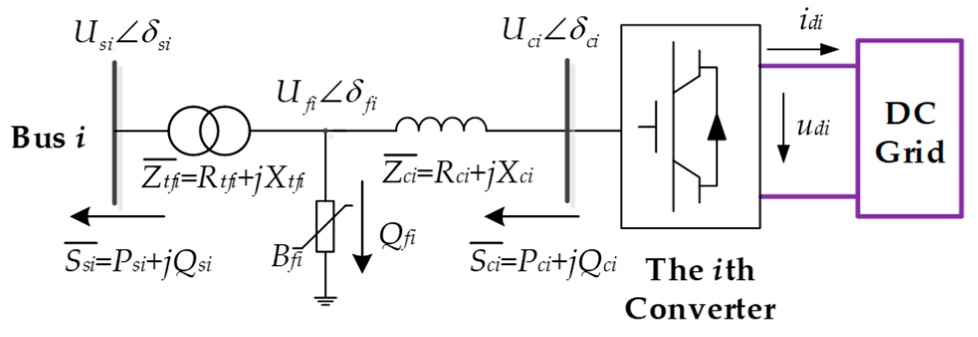
2.1. VSC Model

In general, the i^th VSC in VSC-MTDC is viewed as a controllable voltage source $\overline{U_{\mathit{ci}}}{=U}_{\mathit{ci}}\angle {\delta }_{\mathit{ci}}$ with connecting an impedance $\overline{Z_{\mathit{ci}}}{=R}_{\mathit{ci}}{+\mathit{jX}}_{\mathit{ci}}$, as shown in Figure 1. Then, the converter is connected with a filter and a transformer. The AC bus i is connected with the filter B_fi through the transformer represented by $\overline{Z_{\mathit{tfi}}}{=R}_{\mathit{tfi}}{+\mathit{jX}}_{\mathit{tfi}}$. The apparent power from the converter and flowing to AC bus $\overline{U_{\mathit{si}}}{=U}_{\mathit{si}}\angle {\delta }_{\mathit{si}}$, respectively, are $\overline{S_{\mathit{ci}}}{=P}_{\mathit{ci}}{+\mathit{jQ}}_{\mathit{ci}}$ and $\overline{S_{\mathit{si}}}{=P}_{\mathit{si}}{+\mathit{jQ}}_{\mathit{si}}$. The equations of the power flow injecting to AC bus can be expressed as [23]:

$$\{\begin{array}{l}{P}_{si}=-U_{si}^2{G}_{tfi}^{}+U_{si}^{}{U}_{fi}^{}[G_{tfi}^{}\cos ({\delta }_{si}^{}-{\delta }_{fi}^{})+B_{tfi}^{}\sin ({\delta }_{si}^{}-{\delta }_{fi}^{})]\hfill \\ Q_{si}=U_{si}^2{B}_{tfi}^{}+U_{si}^{}{U}_{fi}^{}[G_{tfi}^{}\sin ({\delta }_{si}^{}-{\delta }_{fi}^{})-B_{tfi}^{}\cos ({\delta }_{si}^{}-{\delta }_{fi}^{})]\hfill \end{array},$$

(1)

where $\overline{U_{\mathit{fi}}}=U_{\mathit{fi}}\angle {\delta }_{\mathit{fi}}$ is the voltage at the filter.

The corresponding equations of power flowing from the i^th converter can be written as:

$$\{\begin{array}{l}{P}_{ci}=U_{ci}^2{G}_{ci}^{}-U_{ci}^{}{U}_{fi}^{}[G_{ci}^{}\cos ({\delta }_{fi}^{}-{\delta }_{ci}^{})-B_{ci}^{}\sin ({\delta }_{fi}^{}-{\delta }_{ci}^{})]\hfill \\ Q_{ci}=-U_{ci}^2{B}_{ci}^{}+U_{ci}^{}{U}_{fi}^{}[G_{ci}^{}\sin ({\delta }_{fi}^{}-{\delta }_{ci}^{})-B_{ci}^{}\cos ({\delta }_{fi}^{}-{\delta }_{ci}^{})]\hfill \end{array}.$$

(2)

The filter generates the reactive power which can be expressed as:

$$Q_{fi}=-U_{fi}^2{B}_{fi}^{}.$$

(3)

The active power balance of the i^th converter can be written as:

$$P_{ci}+P_{DCi}+P_{Loss\_i}=0.$$

(4)

Generally, the $P_{\mathit{DCi}}$ is determined as:

$$P_{Dci}=u_{di}{\displaystyle \sum _{\begin{array}{l}j=1\\ j\ne i\end{array}}^n{Y}_{dij}}\times (u_{di}-u_{dj}),$$

(5)

where u_di is the DC voltage at the i^th converter, and Y_dij is the conductance matrix of DC grids.

The can be obtained by:

$$P_{L\mathrm{oss}\_i}=K_A+K_B{I}_{ci}+K_C{I}_{Ci}^2,$$

(6)

where K_A, K_B, and K_C are constant parameters in [23], and $I_{\mathit{ci}}$ is the AC current magnitude.

2.2. Control Modes of VSC

To keep the active power balance of VSC-MTDC system, at least one VSC should be selected as an active power regulator with using the constant $u_{\mathit{di}}$ control mode. The control modes of VSC are shown as follows:

(1)

the constant $u_{\mathit{di}}$, Q_si control ($u_{\mathit{di}}-Q_{\mathit{si}}$);

(2)

the constant $u_{\mathit{di}}$, U_si control ($u_{\mathit{di}}-U_{\mathit{si}}$);

(3)

the constant P_si, Q_si control ($P_{\mathit{si}}-Q_{\mathit{si}}$);

(4)

the constant P_si, U_si control ($P_{\mathit{si}}-U_{\mathit{si}}$).

In a practical power system, the increasing WFs are integrated into the main AC grid through the advanced VSC-MTDC system. Unfortunately, the output power of WFs generally varies. The constant control modes shown above are not suitable for the VSCs on WF side (WFVSC). To handle this problem, a dual-mode control strategy (DMC) is introduced for WSVSC in [24]. DMC control mode cannot only actively adjust the VSC to adapt the varying output of a WF but also has the ability to maintain the voltage of the WSVSC AC, thus improving the frequency and voltage stability of the WFs. Hence, the DMC control mode is adopted in case studies of this paper. The detailed control modes and methods can be accessed in [25,26].

2.3. Power Flow Calculation for Hybrid AC/VSC-MTDC Grids

The DPF problem of the hybrid AC/VSC-MTDC grid is usually solved by using the sequential method. In [24], the detailed procedures of DPF calculation for hybrid AC/VSC-MTDC were given. Actually, the DPF calculation for hybrid AC/DC grids can be viewed as an implicit function with multi-dimensional random input and output variables, which can be expressed as:

Y = H(X),

(7)

where X represents input variables (such as loads, traditional generation and WFs’ output power), while Y denotes output variables that mainly includes the voltages and branch flow of AC and DC grids. Therefore, if the randomness of wind power and load in hybrid AC/VSC-MTDC grid is considered, the model above will become a PPF problem.

3. Ninth-Order Polynomial Normal Transformation for Random Inputs Modeling

The uncertain sources like wind speeds are affected by diverse factors such as meteorological and geographical conditions, and hence they may not follow the common distributions but being subject to irregular distributions. Meanwhile, the correlations amongst these variables cannot be neglected. In this section, the NPNT is introduced to handle this problem based on historical records.

3.1. Polynomial Coefficients Evaluation for Modeling the Uncertainties

The key idea of polynomial normal transformation lies in that polynomial arithmetic of standard normal random variable is used to model random variable following arbitrary distribution. According to [13], the ninth-order polynomial normal transformation can be formulated as

$$\{\begin{array}{l}{x}_o={\mu }_x+{\sigma }_x{x}_{}\hfill \\ x_{}=a_0+a_{1}z+\cdots +a_k{z}^k+\cdots +a_9{z}^9\hfill \end{array},$$

(8)

where $x_o$ is a continuous random variable in practical power grid like wind speeds, ${\mu }_x$ and ${\sigma }_x$ are mean and standard deviation value of input uncertain variables, respectively, $x$ denotes the normalized random variable. $z$ is a standard normal random variable, and $a_k$ ($k$ = 1, 2, …, 9) are the undetermined coefficients. If the suitable $a_k$ ($k$ = 1, 2, …, 9) are obtained, the stochastic variables following irregular distributions can be stimulated.

In general, the statistical moments are used to denote the data characteristics of random variables. The probability weighted moment (PWM) in this paper is used to characterize the uncertainties. Reference [27] presents a method to obtain the PWMs of uncertain input variables by using historical records of uncertainties. Sorting the input random variables into an ascending order $x_1\le \cdots \le x_i\cdots \le x_n$, the PWM ${\beta }_r$ can be solved by

$${\beta }_r=\frac{1}{n}{\displaystyle \sum _{i=r+1}^n\frac{(i-1)(i-2)\cdots (i-r)}{(n-1)(n-2)\cdots (n-r)}}{x}_i.$$

(9)

The first 10 PWMs (${\beta }_0{-\beta }_9$) of random variables can be calculated by Equation (9). By using Equations (10) and (11), the polynomial coefficients $a_k$ ($k$ = 0, 1, …, 9) can be easily obtained.

$$A_{r,k}^z={\displaystyle {\int }_{-\infty }^{+\infty }{z}^k\cdot {\mathsf{\Phi }}^r\left(z\right)\cdot \phi \left(z\right)dz}$$

(10)

$$\left(\begin{array}{ccccc}{A}_{0,0}^z& \cdots & A_{0,k}^z& \cdots & A_{0,9}^z\\ ⋮& \cdots & ⋮& \cdots & ⋮\\ A_{r,0}^z& \cdots & A_{r,k}^z& \cdots & A_{r,9}^z\\ ⋮& \cdots & ⋮& \cdots & ⋮\\ A_{9,0}^z& \cdots & A_{9,k}^z& \cdots & A_{9,9}^z\end{array}\right)\cdot \left(\begin{array}{c}{a}_0\\ ⋮\\ a_k\\ ⋮\\ a_9\end{array}\right)=\left(\begin{array}{c}{\beta }_0\\ ⋮\\ {\beta }_k\\ ⋮\\ {\beta }_9\end{array}\right),$$

(11)

where $\mathsf{\Phi }\left(z\right)$ and $\phi \left(z\right)$, respectively, are the cumulative distribution function (CDF) and PDF of the standard normal variable. $A_{r,k}^z$ (r = 0, 1, …, 9; k = 0, 1, …, 9) is a constant value which can be evaluated by numerical integration. Note that the polynomial coefficients of NPNT can be easily obtained, as Equation (11) is linear.

3.2. Correlation Coefficients Estimation in Standard Normal Space

Generally, the correlations among uncertain sources cannot be ignored. Suppose that $x_1$, $x_2$ are two correlated and normalized random variables following arbitrarily distributions. Using the procedure of polynomial coefficients calculation introduced above, $x_1$ and $x_2$ can be expressed as

$$\begin{array}{c}{x}_1=a_{1,0}+\dots +a_{1,i}{z}_1^i+\dots +a_{1,9}{z}_1^9\\ x_2=a_{2,0}+\dots +a_{2,i}{z}_2^i+\dots +a_{2,9}{z}_2^9\end{array}$$

(12)

If the correlation coefficient ${\rho }_z$ between $z_1$, $z_2$ (following standard normal distributions) can be determined, the correlated $x_1$, $x_2$ can be simulated by using correlated standard normal random variables. To obtain the ${\rho }_z$ the functional relationship between ${\rho }_x$ and ${\rho }_z$ is established, which is

$$\begin{array}{cc}\hfill {\rho }_x{\sigma }_1{\sigma }_2+{\mu }_1{\mu }_2& =E\left(x_1{x}_2\right)\hfill \\ & =E\left[\left({\displaystyle \sum _{i=0}^9{a}_{1,i}{z}_1^i}\right)\left({\displaystyle \sum _{j=0}^9{a}_{2,i}{z}_2^j}\right)\right]\hfill \end{array}$$

(13)

where ${\mu }_r$ and ${\sigma }_r$ are the means and standard deviations of $x_r$ (r = 1, 2), respectively.

The product moments ${E(z}_1^i{z}_2^j)$ can be expressed as a polynomial of ${\rho }_z$ which is introduced in detail in [13]. Note that the correlation coefficient ${\rho }_x$ between $x_1$, $x_2$ can be obtained by historical records. Hence, the correlation coefficient ${\rho }_z$ can be determined by solving Equation (13).

3.3. NPNT for Modeling Multiple Random Variables in Hybrid AC/VSC-MTDC Grid

Actually, the normalized m-dimension random variable $x_i$ in X can be formulated as $x_i={{\displaystyle \sum }}_{k=0}^9{a}_{i,k}{z}_i^k$. Then, based on the ρ_x(i,j) of ${\mathit{R}}_{\mathit{X}}{=[\rho }_x{(i,j)]}_{i,j=1}^n$, the ρ_z(i,j) (i≠j) of ${\mathit{R}}_{\mathit{Z}}{=[\rho }_z{(i,j)]}_{i,j=1}^n$ can be easily obtained. Note that R_Z is the equivalent correlation matrix of R_X in the standard normal space. Then, random matrix X can be simulated by:

(1)

obtain the standard normal random variables $\mathit{Z}$ with the correlation matrix ${\mathit{R}}_{\mathit{Z}}$;

(2)

calculate the correlated multivariate random vector X by using correlated standard normal vector $\mathit{Z}$.

The detailed procedures of modeling multiple random variables by NPNT can be accessed in [13]. The key advantage of using NPNT in PPF analysis for AC/VSC-MTDC grids lies in that NPNT merely uses historical records of uncertain sources without assuming the PDFs of uncertainties in advance. That is to say, it is able to accurately handle correlated random variables, regardless of whether the underlying distribution is known or unknown.

4. Inherited Latin Hypercube Sampling Technique

The powerful NPNT can be adopted to build an accurate probability model of random inputs based on practical recordings. Then, the next crucial step is to propagate the randomness from inputs to target outputs by using the sampling technique with the DPF model of hybrid AC/VSC-MTDC grid. In this section, the CLHS is briefly introduced, followed by the detailed introduction of ILHS.

4.1. Conventional Latin Hypercube Sampling Technique

In general, the sampling and permutation are the two major steps of CLHS [19]. The purpose of sampling is to obtain representative samples that could reflect the distribution regions of input random variables, and then the permutation technique is used to control the correlation of generated samples. The q^th CDF F_q value of input variables X_p,q ranges from 0 to 1, which is divided into $P^{\mathit{num}}$ non-overlapping intervals. Note that $P^{\mathit{num}}$ (1, 2, …, p) donates sample size, and $Q^{\mathit{num}}$ (1, 2, …, q) represents the number of input variables. The procedure of CLHS is given below.

Procedure 1: CLHS

1. Sampling: (1) Generate a random matrix with uniform distribution U = [up,1, up,2, …, up,q].

(2) Obtain the sample point matrix on uniform distribution R = [rp,1, rp,2, …, rp,q] by using rp,q = (p − up,q).

(3) The sample values on the qth original distribution can be obtained by Xp,q = $F_q^{-1}$ (rp,q). 2. Permutation (1) Cholesky decomposition is adopted herein to obtain the permutation matrix of sample points, making the correlations trend closer to theoretical values [28].

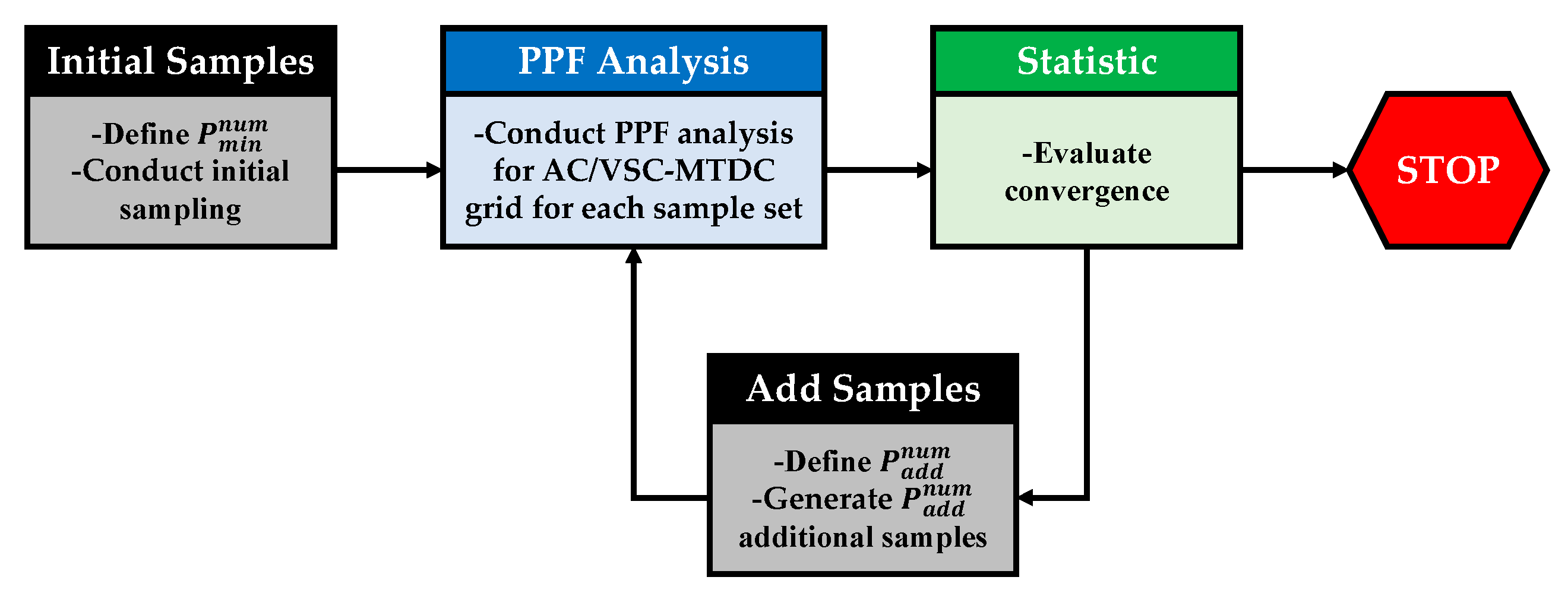
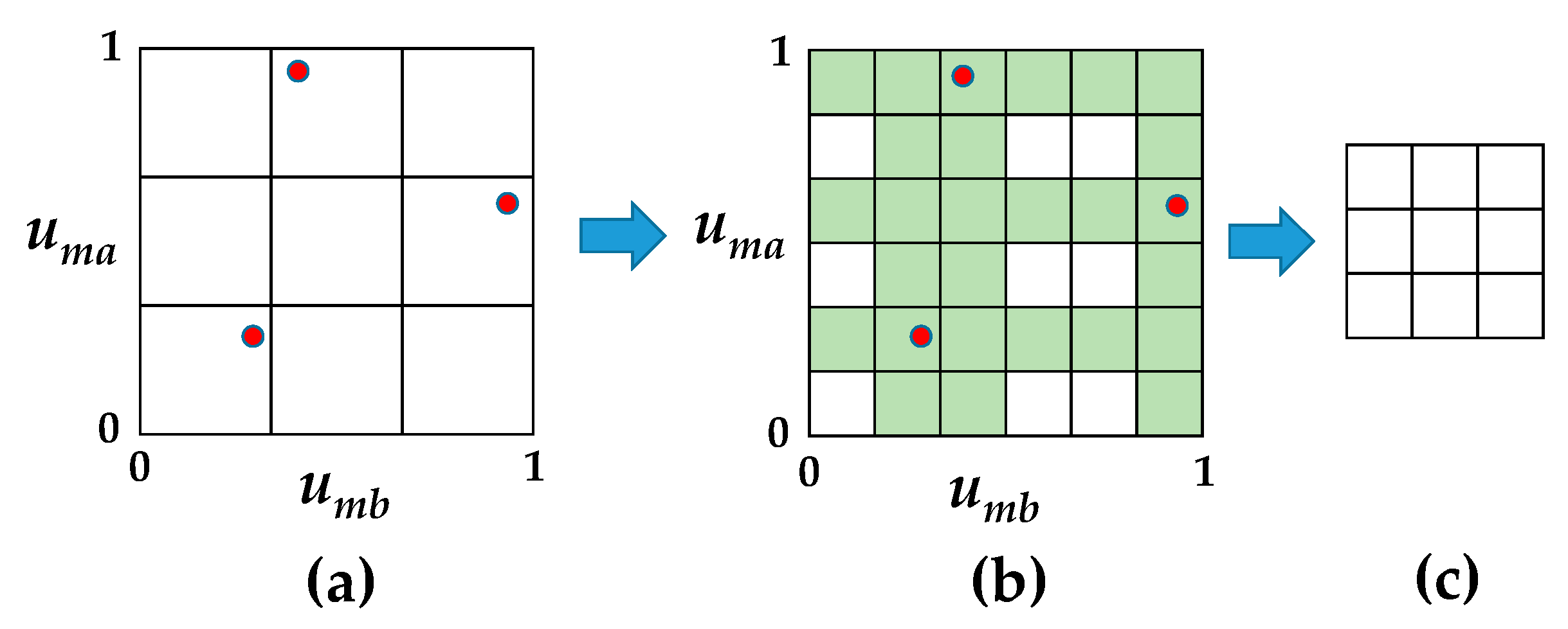
4.2. Inherited Latin Hypercube Sampling Design

It is well-known that CLHS exhibits higher computational speed than the MCS method. However, the drawback of CLHS lies in that its highly structured form makes it difficult to directly add extra samples to an already generated sample matrix [21]. This naturally leads to a question regarding how many samples are sufficient in PPF analysis for the complex hybrid AC/VSC-MTDC grid based on CLHS. Actually, a small sample may not guarantee accurate PPF results, while a large sample will decrease the computational efficiency. Therefore, the extension work makes sense to further improve the computational flexibility of CLHS.

Figure 2 shows the schematic diagram of the ILHS method. The basic idea of ILHS lies in that it is desirable to start with a small sample size for conducting PPF analysis of a hybrid AC/VSC-MTDC grid as an initial step and then gradually extend the sample size if deemed necessary. As well known, refining the existing sample matrix instead of recreating a totally new one could reuse obtained CLHS’s results, leading to a significant improvement in the computational efficiency for PPF analysis. This is extremely meaningful for PPF analysis of the hybrid AC/VSC-MTDC grid since DPF simulation of the hybrid AC/VSC-MTDC grid is more expensive than the pure AC grid. Meanwhile, based on a given convergence criterion for a specific operational scenario of the hybrid AC/VSC-MTDC grid, the ILHS could adaptively change the sample size, thus obtaining higher computational accuracy and efficiency. Furthermore, the moments and PDFs can also be accurately and directly obtained by use of ILHS.

To illustrate the key idea of ILHS, the two variables u_ma, u_mb following uniform distributions are defined. It is assumed that three sample points are generated in the first step by using CLHS, as shown in Figure 3a. The next step for ILHS is to generate new sample points while inheriting obtained sample points. It is assumed that six sample points are needed. That is to say, three additional sample points should be generated by ILHS. The variables u_ma, u_mb can be divided into six non-overlapping intervals, as shown in Figure 3b. The spaces represented by the inherited sample points are shaded with green. If shaded spaces are removed from Figure 3b, the unrepresented variable space will emerge as a blank space, as shown in Figure 3c.

Actually, the three additional sample points can be filled into the blank space in Figure 4a. By using CLHS, the positions of the three additional sample points can be easily determined. It can be observed that inherited sample points (denoted by red dots) and the additional sample points (represented by black square dots) form the new sample set covering the input probability space more evenly and largely, as shown in Figure 4b. Then, these new sample sets can be permutated and transformed into the original probability space. It is valuable to note that, in PPF analysis based on ILHS, the obtained PPF results corresponding to inherited sample points can be reused, thus resulting in the improvement of accuracy while retaining the computational efficiency. The main implement steps of ILHS in handling multiple variables are elaborated as Algorithm 1 [22].

Algorithm 1: ILHS

NOTE: it is assumed that the PPF analysis based on CLHS has been executed as the first step with using the sample size $P^{\mathit{num}}$. Hence, the inherited sample set ${\mathit{U}}_{}^{}=\left[{\mathit{u}}_{\mathit{p},\mathbf{1}}^{}, {\mathit{u}}_{\mathit{p},\mathbf{2}}^{}, \dots ,{\mathit{u}}_{\mathit{p},\mathit{q}}^{}\right]$ is viewed as the input variables in ILHS. Procedure: (1) C_criterion = 1. (2) k = 2, where k represents the iterations. (3) While C_criterion = 1. (4) Divide the uniform distributions into kP intervals with equal probability. (5) Generate sample points in unrepresented variable space. (6) Obtain the new sample set ${\mathit{U}}_{}^{\mathit{new}}=\left[{\mathit{u}}_{\mathit{k}\mathit{p},\mathbf{1}}^{}, {\mathit{u}}_{\mathit{k}\mathit{p},\mathbf{2}}^{}, \dots ,{\mathit{u}}_{\mathit{k}\mathit{p},\mathit{q}}^{}\right]$ on uniform distributions. (7) The new sample set is permutated by using Cholesky decomposition. (8) Select the samples in the unrepresented variable space and transform these samples into original probability space. (9) Feed the transformed samples into DPF module of hybrid AC/VSC-MTDC grids. (10) Analyze the results (the results include the newly obtained and inherited PPF outputs). (11) If $\left|(I_Y^k-I_Y^{k-1})/I_Y^k\right|\le \beta$, where $I_Y^k$ denotes the statistical moments of PPF outputs after the kth extension, $\beta$ represents the threshold value. (12) C_criterion = 0 (13) Else (14) k = k + 1; (15) End (16) End

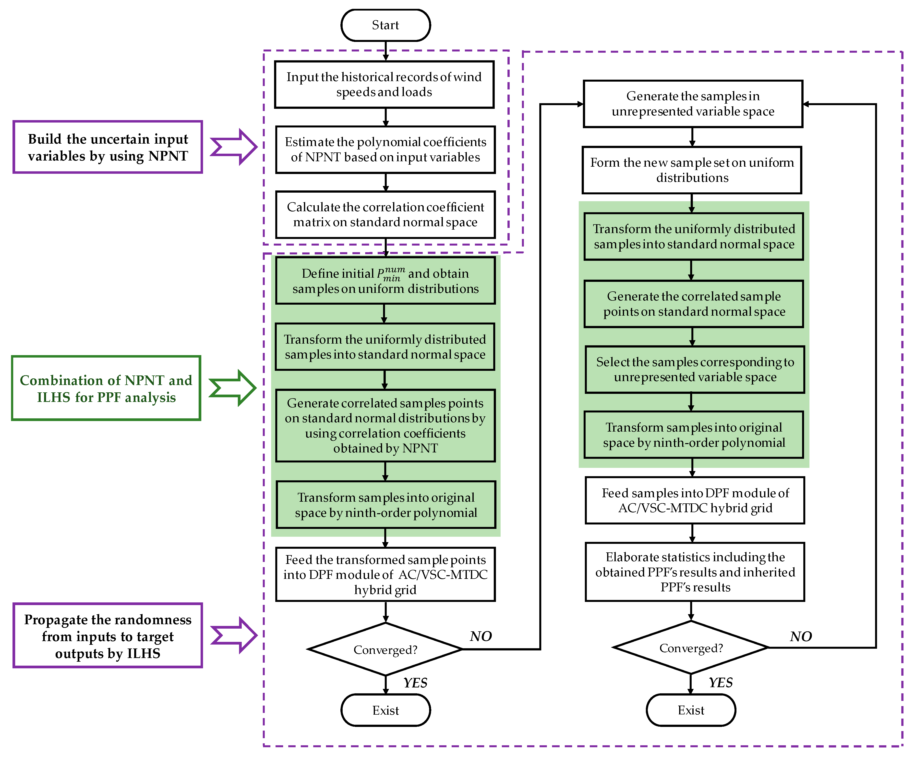
5. Combination of NPNT and ILHS for PPF Analysis of Hybrid AC/VSC-MTDC Grid

The procedures of combining NPNT and ILHS for conducting PPF analysis on a hybrid AC/VSC-MTDC grid is presented in Figure 5. As the initial step for PPF analysis, modeling of random inputs is critical. However, the direct information about probabilistic characteristics of inputs is rather limited in realistic engineering applications, while the raw statistical data is more or less available in practice; moreover, even if raw data is sufficient for fitting the PDF but not always in a common PDF type, thus leading to an accuracy loss. Therefore, NPNT is used to handle the raw statistical data and build the probability model of random inputs.

Once the accurate input probability model is built, the next step is to propagate the randomness from the input probability model to target outputs by means of ILHS. The steps of combining TPNT and CLHS methods are introduced in [11]. The similar idea can be applied to the combination of NPNT and ILHS herein as well. In addition, the basic idea of combining NPNT and CLHS or ILHS methods is summarized as (1) obtain the samples on uniform distributions; (2) transform these samples into standard normal space; (3) transform the samples of standard normal space into original space by using ninth-order polynomial. The core steps are highlighted in the green part of Figure 5. The advantages of the proposed method are shown below.

(1)

The proposed method can deal with the random variables following irregular distributions even with correlations merely based on historical records.

(2)

The results obtained in the previous simulations can be reused by the proposed method, thus improving the computational speed and efficiency.

(3)

The proposed method has a better adaptability and flexibility for diverse operational scenarios of the complex AC/VSC-MTDC grids as it is able to adaptively evaluate sample size adequacy, based on an acceptable accuracy.

(4)

The statistical moments (such as means and standard deviations) and PDFs of PPF results could be accurately and directly obtained by use of the proposed method.

6. Case Studies

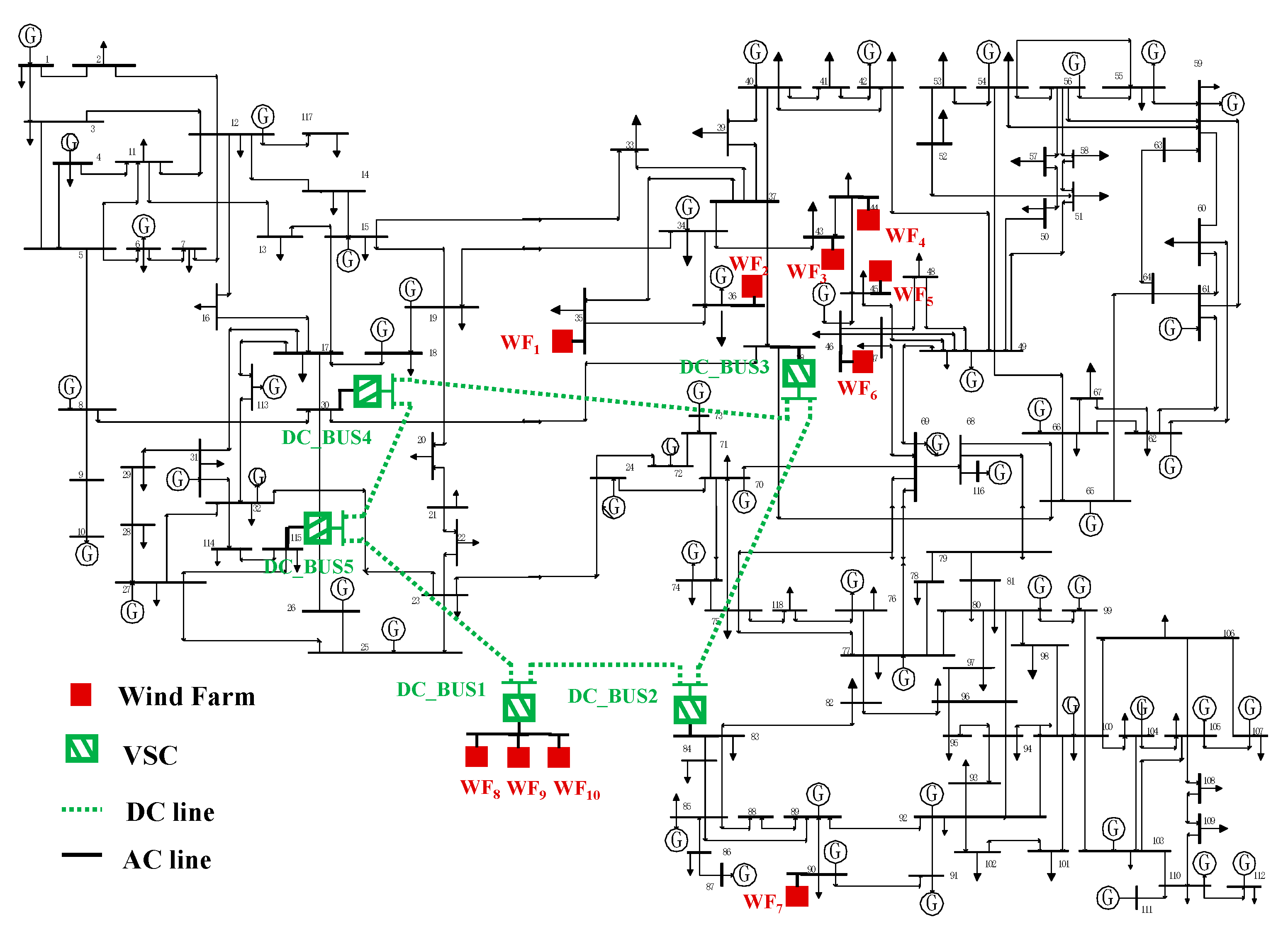
6.1. System, Data, and Scenarios

The modified IEEE 118-bus system was applied in this paper to demonstrate the effectiveness and superiority of the proposed method. As shown in Figure 6, seven additional wind farms (including WF₁, WF₂, WF₃, WF₄, WF₅, WF₆, and WF₇) were added to the modified IEEE 118-bus system respectively at buses 35, 36, 43, 44, 45, 46, and 90. Meanwhile, the wind farms WF₈, WF₉, and WF₁₀ were connected to the AC grid at bus 30, 38, 84, and 115 through a five-terminal DC grid incorporating VSCs. The parameters of the IEEE 118-bus system can be found in Matpower 6.0 [29]. The parameters of the VSCs and DC lines are given in [3]. In this paper, the control modes of the VSCs are presented in

Table 1. Control modes of VSCs.

DC Bus	Control Modes	udi (p.u)	Usi (p.u)	Psi (p.u)	Qsi (p.u)
1	DMC	\	1.00	\	\
2	$P_{\mathit{si}}-Q_{\mathit{si}}$	\	\	0.98	0.3
3	$u_{\mathit{di}}-Q_{\mathit{si}}$	1.00	\	\	0.38
4	$P_{\mathit{si}}-U_{\mathit{si}}$	\	1.00	0.65	\
5	$P_{\mathit{si}}-Q_{\mathit{si}}$	\	\	0.65	0.3

. Note that the base power of the AC and DC grids were set to be 100 MVA.

In a practical power system, different areas may have different types of loads with diverse characteristics and following various distributions. In this paper, it was assumed that the loads in the test system can be categorized into three groups: commercial load, industrial load, and residential load. Assumed that the same type of load has a similar probability characteristic. In order to simulate the probability characteristic of such practical loads, the realistic historical records of commercial load, industrial load, and residential load in a southern provincial power grid of China were used. The procedures for modeling different types of loads are given in Appendix A. The types of loads in the test system are presented in

Table 2. Types of loads at different buses in the modified IEEE 118-bus system.

	Commercial Loads	Industrial Loads	Residential Loads
Locations	Loads at buses 75, 76, 77, 78, 79, 80, 82, 83, 84, 85, 86, 88, 90, 91, 92, 93, 94, 95, 96, 97, 98, 99, 100, 101, 102, 103, 104, 105, 106, 107, 108, 109, 110, 112, 116, and 118	Loads at buses 1, 2, 3, 4, 6, 7, 8, 11, 12, 13, 14, 15, 16, 17, 18, 19, 33, 34, 35, 36, 39, 40, 41, 42, 43, 44, 45, 46, 47, 48, 49, 50, 51, 52, 53, 54, 55, 56, 57, 58, 59, 60, 62, 66, 67, 74, 113, 115, and 117	Loads at buses 20, 21, 22, 23, 24, 27, 28, 29, 31, 32, 70, 72, 73, and 114

.

The realistic wind speeds may not follow common distributions like Weibull distributions. The data of wind speeds are based on historical records in a southern provincial power grid of China, which is applied to the wind farms in this case study. An emphasis is put on that the historical records of wind speed and load are collected from the same area. It was assumed that the correlation coefficients amongst wind speeds at wind farms WF₁, WF₂, WF₃, WF₄, WF₅, WF₆, and WF₇ were 0.3, and correlation coefficients amongst wind speeds at wind farms WF₈, WF₉, and WF₁₀ were 0.4. Moreover, assuming that the correlation coefficients among commercial loads were set to be 0.2, the correlation coefficients among residential loads were 0.25, and the correlation coefficients between any two industrial loads were set to be 0.1. The rated capacities of these wind farms were set to 100 MW, and the power factors of these wind farms were set to be 0.95. The wind farm output model in 7 was applied in this case study.

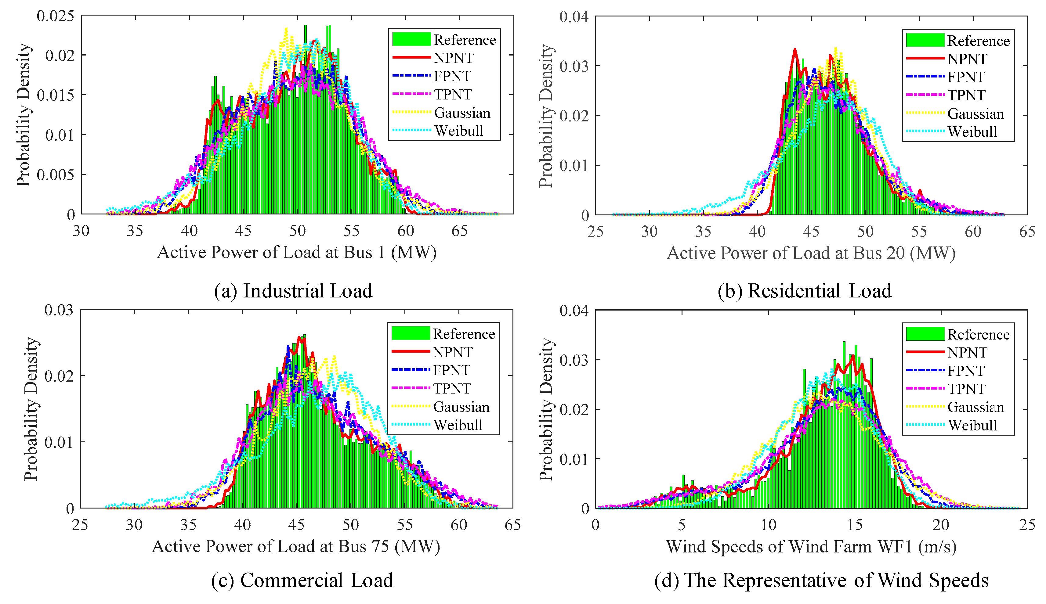
6.2. Performance Evaluation on Probability Model of Random Inputs

The frequency histogram was applied as a major metric to evaluate the accuracy of NPNT for modeling of uncertain inputs. A frequency histogram similarity index (FHSI) [30] was used in this paper to denote the degree of overlap between any two frequency histograms obtained by means of reference method and the methods in comparison, which is

$$FHSI=\left(1-\frac{1}{2}{\displaystyle \sum _{i=1}^{N_s}[{(Bi{n}_i^{reference}-Bi{n}_i^{compared})}_{}^2+{(Pe{r}_i^{reference}-Pe{r}_i^{compared})}_{}^2{]}_{}^{\frac{1}{2}}}\right)\times 100\%,$$

(14)

where ${\mathit{Bin}}_i^{\mathit{reference}}$ and ${\mathit{Bin}}_i^{\mathit{compared}}$ respectively are the values of locations of each Bin interval, while ${\mathit{Per}}_i^{\mathit{reference}}$ and ${\mathit{Per}}_i^{\mathit{compared}}$ denote percentages of the number of samples fall in each Bin interval. $N_s$ represents the number of Bin intervals. Actually, the number of Bins in frequency histogram must be identical, and 100 was applied for all tests in this paper. The range of FHSI is between 0 and 1. A larger FHSI represents that the obtained frequency histogram is closer to the reference’s, indicating the higher accuracy is achieved in terms of modeling uncertain variables. FHSI >90% is regarded as “accurate” in this paper.

In order to evaluate the performance of NPNT, the frequency histograms of loads and wind speeds obtained by historical records were regarded as the references for validation. To further demonstrate the superiority of NPNT, the results fit by NPNT were compared with those obtained from TPNT, FPNT, Gaussian, and Weibull distributions. The Gaussian and Weibull distributions were frequently used in the probabilistic analysis of the power system, which were directly applied to fit the historical records in this paper. Note that the number of samples of historical records is 9000; accordingly, in Figure 7, NPNT, FPNT, TPNT, Gaussian, and Weibull distributions generate 9000 samples as well for a fair comparison.

Figure 7 presents the frequency histograms of the active power of load at bus 1, bus 20, bus 75, and wind speeds obtained by historical records, NPNT, FPNT, TPNT, Gaussian, and Weibull distributions. Obviously, the frequency histograms obtained by historical records cannot be fitted well with Gaussian and Weibull distributions. The reason for this lies in that the random variables in the practical power system may not follow common distributions but irregular distributions. Furthermore, frequency histograms obtained using FPNT and TPNT are biased compared with the reference results obtained by using historical records. Meanwhile, it is obvious that the frequency histograms of NPNT can fit very well with the frequency histograms of reference results. Compared with FPNT and TPNT, NPNT has the ability to control the first to tenth moments of historical records, leading to the improvement in the accuracy of modeling random inputs.

The accuracy index FHSIs obtained by NPNT, FPNT, TPNT, Gaussian, and Weibull distributions also support the conclusions given above, as shown in

Table 3. Frequency histogram similarity indexes (FHSIs) obtained by NPNT, FPNT, TPNT, Gaussian, and Weibull distributions.

Methods, The Number of Samples	NPNT, 9000	FPNT, 9000	TPNT, 9000	Gaussian, 9000	Weibull, 9000
Load at bus1	94.36%	88.70%	86.92%	85.74%	86.42%
Load at bus20	94.01%	88.66%	85.62%	85.03%	76.48%
Load at bus75	94.34%	90.37%	87.28%	85.63%	78.61%
WF1	92.87%	85.05%	81.43%	76.66%	83.29%
WF2	94.05%	90.05%	88.05%	74.32%	84.05%
WF3	94.32%	88.32%	86.32%	78.19%	83.25%
WF4	93.28%	89.28%	87.28%	76.24%	83.28%
WF5	94.21%	90.21%	86.21%	77.36%	82.21%
WF6	93.92%	90.92%	87.92%	79.56%	84.92%
WF7	93.61%	89.61%	87.61%	74.23%	83.61%
WF8	94.49%	90.49%	86.49%	79.12%	82.49%
WF9	93.89%	89.89%	87.89%	72.26%	83.89%
WF10	93.59%	90.59%	87.59%	75.46%	84.59%

. Using common distributions (such as Gaussian and Weibull distributions) may not fit well with frequency histograms obtained by historical records in practice. For example, the maximum and average values of FHSIs obtained Gaussian and Weibull distributions respectively are 85.74%, 78.45% (for Gaussian distribution) and 86.42%, 82.85% (for Weibull distribution). The average values of FHSIs obtained by NPNT, FPNT, and TPNT, respectively, are 93.92%, 89.40%, and 86.66%. Actually, most FHSIs of NPNT are greater than 93.5%, qualifying the NPNT as “accurate.” NPNT allows the accuracy control of higher-order moments, which yields a more accurate simulation of input random variables. Hence, in the next section, NPNT is applied to simulate correlated random variables in PPF analysis.

6.3. Performance Evaluation of Proposed PPF Method

In this section, the performance of the proposed PPF method will be comprehensively evaluated. The reference results are obtained by using the MCS based NPNT method, in which the MCS generates 50,000 sample points. It is sufficient to yield reliable PPF results. The proposed method in this paper is combined NPNT with ILHS, which is denoted as NPNT-ILHS.

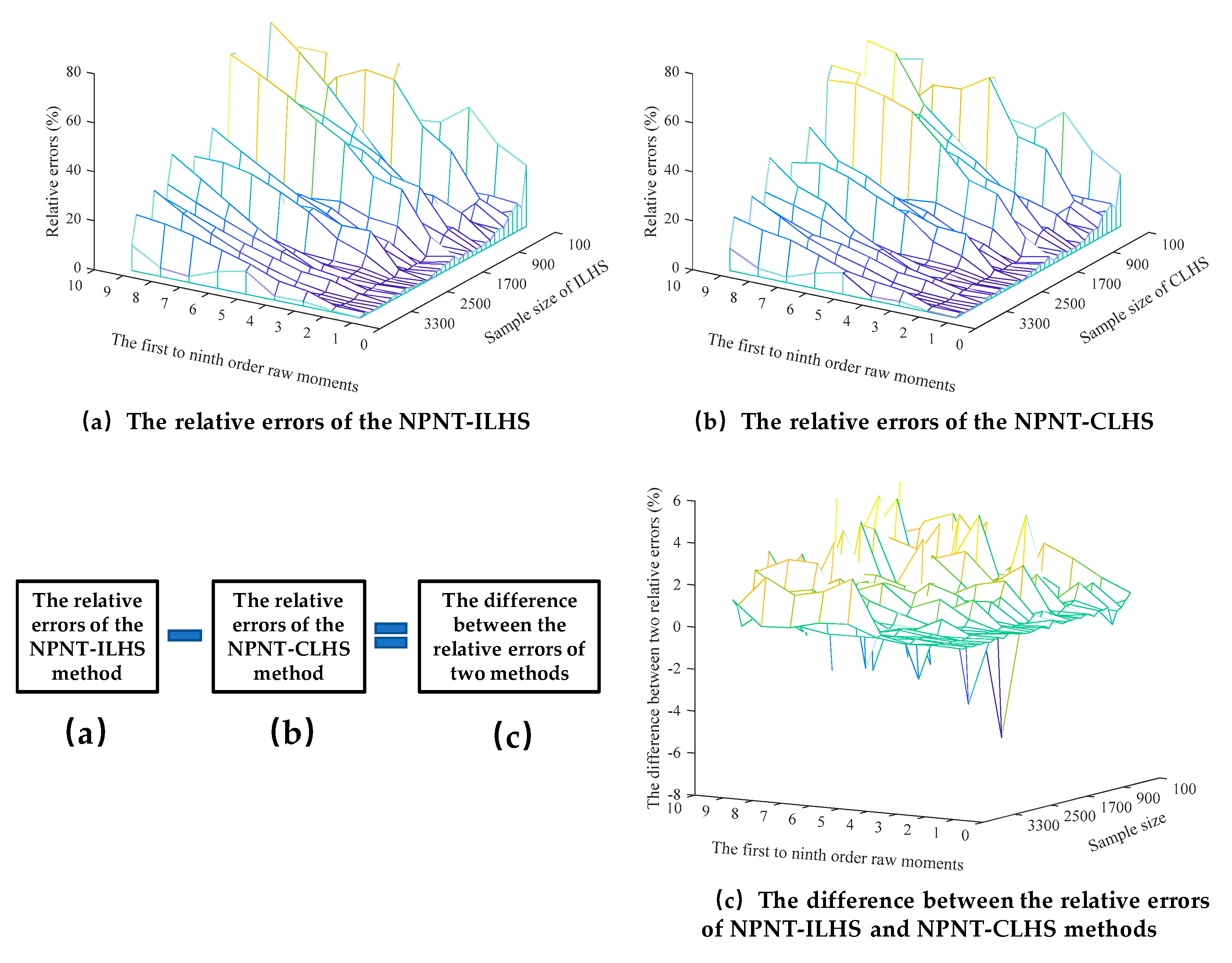
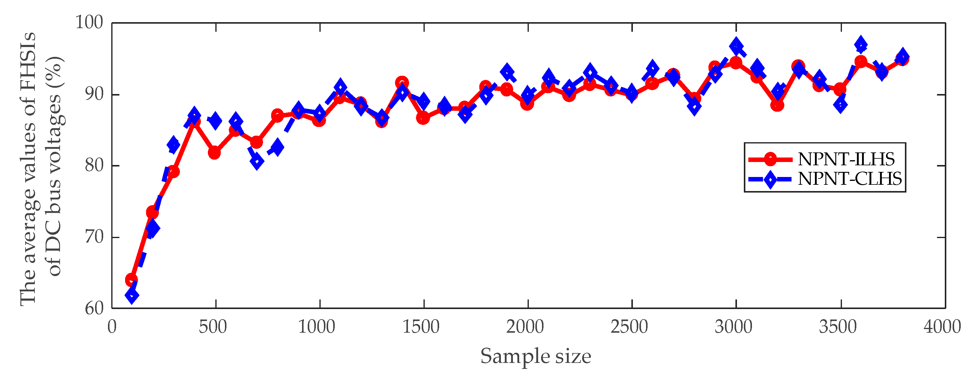
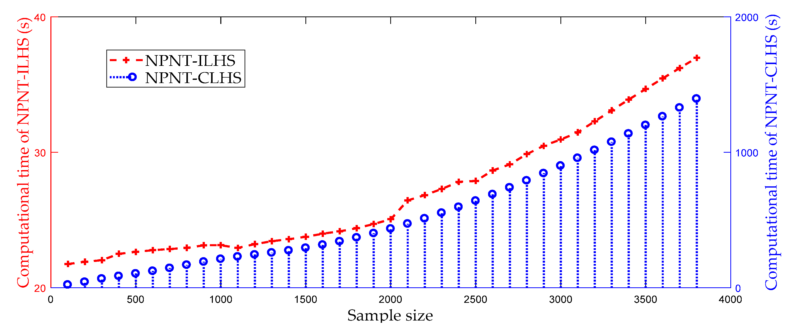
6.3.1. Comparison with the CLHS Method

In this subsection, the CLHS is combined with NPNT to form the NPNT-CLHS method for comparison. The proposed method NPNT-ILHS adds 100 samples in each iteration until convergence is reached. The average value of the first to ninth order raw moments of VSC3′s output active power is set to be the convergence criterion; meanwhile, the threshold value is set to 5%.

The relative errors of the first to ninth raw moments of VSC3′s output active power obtained by using NPNT-ILHS and NPNT-CLHS methods are shown in Figure 8. Meanwhile, Figure 9 presents the average values of FHSIs of DC bus voltages corresponding to different sample sizes. It can be investigated that the computational accuracy of the NPNT-CLSH method and proposed method NPNT-ILSH are almost the same. The difference between the relative errors of the first to ninth raw moments of VSC3′s output active power is given in Figure 8c. Obviously, most of the values in Figure 8c are smaller than 4%. With using 3600, 3700, and 3800 samples, the average values of FHSIs of DC bus voltages, respectively, are 94.32%, 92.15%, and 94.07% for NPNT-CLHS while 94.09%, 92.47%, and 93.89% for NPNT-ILHS (as shown in Figure 9). The numerical results indicate that the computational accuracy of the proposed method is very close to the NPNT-CLSH’s. On the other hand, it can be found in Figure 8a,b and Figure 9 that the convergence trend of NPNT-CLHS and NPNT-ILHS methods are nearly identical.

When the samples are increased from 100 to 3800 with an interval 100, the computational time of NPNT-ILSH and NPNT-CLHS methods are shown in Figure 10. When the sample size is 100, 200, 300, 400, and 500, the computational time of NPNT-ILSH and NPNT-CLHS methods, respectively, are 21.75, 21.91, 22.05, 22.24, and 22.51 s for NPNT-ILHS, while 21.71, 42.36, 65.98, 85.75, and 103.89 s for NPNT-CLHS. It can be found from Figure 10 that the computational time of the NPNT-ILHS method is lower than 40 s in each iteration; however, the computational time of the NPNT-CLHS method is higher than 400 s in most trials. The total computational time of the NPNT-ILSH (1021 s) is less than 5% of NPNT-CLHS methods (20,588 s). Evidently, the proposed method NPNT-ILSH can significantly save computational time, compared with the NPNT-CLHS method. The key reason for this lies in that, in PPF analysis, the NPNT-ILHS method can refine the obtained sample matrix and thus reuse the obtained PPF results, leading to the improvement of computational efficiency for PPF calculation. As for the NPNT-CLHS method, however, it could not estimate the reasonable sample size for a specific operational scenario of a hybrid AC/VSC-MTDC grid in advance and thus it needs to repeatedly undertake trials using the total new sample matrix, resulting in an unusually heavy computational burden.

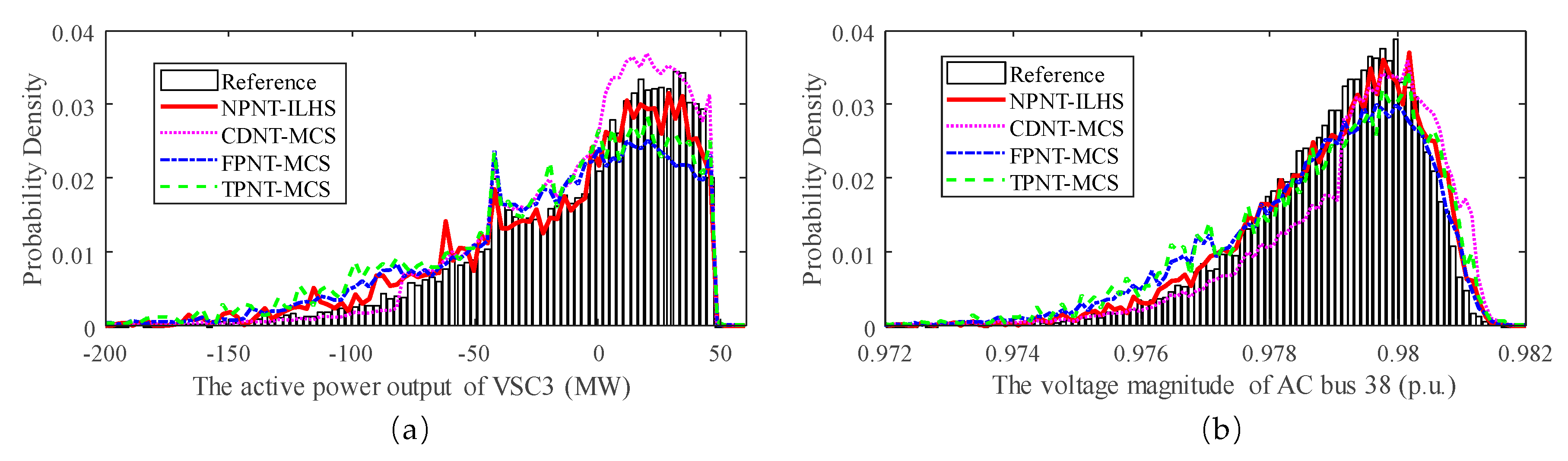
6.3.2. Comparison of PPF Methods with Using Different Input Probability Models

The test in this subsection is mainly used for comparison in terms of computation accuracy. The comparison methods include CDNT-MCS, TPNT-MCS, and FPNT-MCS, as shown in

Table 4. The comparison methods.

Sampling Methods (Sample Size)	Methods of Building the Input Probability Model	Short Name
MCS (50,000)	Common distributions + NATAF transformation	CDNT-MCS
MCS (50,000)	TPNT	TPNT-MCS
MCS (50,000)	FPNT	FPNT-MCS

. These methods use the same sampling method MCS, and the sample size is 50,000. The methods of building input probability model are different. Common distributions and NATAF transformation are used to build the input probability model in CDNT-MCS, while input random variables are handled by using TPNT and FPNT in TPNT-MCS and FPNT-MCS. Note that the convergence criterion and the threshold value are same as the ones of the NPNT-ILHS method presented in Section 6.3.1.

Figure 11 presents the contours of frequency histograms of the VSC3′s active power output and AC bus 38′s voltage magnitude obtained by NPNT-ILHS, CDNT-MCS, TPNT-MCS, and FPNT-MCS methods. Evidently, compared with CDNT-MCS, TPNT-MCS, and FPNT-MCS methods, the proposed method NPNT-ILHS can fit very well with reference’s frequency histogram. As shown in

Table 5. FHSIs obtained by using NPNT-ILHS, CDNT-MCS, FPNT-MCS, and FPNT-MCS.

PPF Methods	VSC3′s Active Power Output	Voltage Magnitude of AC Bus 38	Voltage Magnitude of AC Bus 45	Voltage Magnitude of DC Bus 2
NPNT-ILHS	93.35%	94.16%	93.13%	93.46%
CDNT-MCS	83.37%	84.66%	83.33%	82.15%
FPNT-MCS	88.87%	89.78%	87.93%	87.15%
TPNT-MCS	84.23%	85.78%	85.67%	86.12%

, the FHSIs obtained by using NPNT-ILHS, CDNT-MCS, FPNT-MCS, and FPNT-MCS are presented. The average FHSI values of NPNT-ILHS, CDNT-MCS, FPNT-MCS, and FPNT-MCS method respectively are 93.35%, 83.33%, 88.43%, and 85.45%. The maximum FHSI value of the proposed method NPNT-ILHS achieves 94.16%. Actually, the good performance of the proposed method NPNT-ILHS in PPF analysis is guaranteed, which mainly lies in two reasons. Firstly, the accurate probability model of input variables following irregular distributions can be built based on the NPNT method. This provides a good base for ILHS to propagate the randomness from inputs to target outputs. Secondly, based on a given convergence precision for a specific operational scenario of the hybrid AC/VSC-MTDC grid, the ILHS could adaptively assess the sample size, thus getting higher computational accuracy while holding a good efficiency.

However, frequency histograms obtained by CDNT-MCS, TPNT-MCS, and FPNT-MCS methods are biased compared with those obtained by the reference method in Figure 11. The computation errors of these methods are mainly caused by inaccurate probability model of random input variables. It is demonstrated in Section 6.2 of this paper that the historical records may not follow the common distributions. Hence, the CDNT-MCS method, based on the assumption of input variables following common distributions, will bring error into PPF analysis. Although TPNT-MCS and FPNT-MCS methods build the probability model according to historical records, the frequency histogram of the reference’s result cannot be fitted very well by using these two methods. The FHSIs of voltage magnitude of AC bus 45 of TPNT-MCS and FPNT-MCS methods respectively are 85.67% and 87.93%, which are lower than the FHSI value (93.13%) obtained by proposed method NPNT-ILHS. Moreover, the NPNT has the ability to control the first to the tenth moments of historical records and it is able to build more accurate probability model of inputs, thus leading to an increase in computational accuracy.

6.3.3. Comparison with other PPF Methods

The point estimation method (PEM) is a popular method for solving the PPF problem. In [31], the PEM is combined with TPNT to deal with the PPF problem in pure AC grid. The similar idea can be applied in this paper as well. In this subsection, two PEMs [32] (including 2n+1 PEM and 4n+1 PEM) are combined with NPNT to form the NPNT-2PEM and NPNT-4PEM methods for comparing with proposed method NPNT-ILHS. Meanwhile, two convergence criterions are defined for NPNT-ILHS method to obtain different PPF results with different purposes.

(1)

NPNT-ILHS(a): the convergence criterion for NPNT-ILHS(a) is introduced in Section 6.3.1.

(2)

NPNT-ILHS(b): The average value of the first to third order raw moments of VSC3′s output active power is set to be convergence criterion; meanwhile, the threshold value equals to 5%.

The relative errors of the first to ninth raw moments of DC bus 2′s voltage magnitude is given in

Table 6. The relative errors (%) of the first to the ninth raw moments of DC bus 2′s voltage magnitude.

The Relative Errors (%)	NPNT-ILHS(a)	NPNT-ILHS(b)	NPNT-2PEM	NPNT-4PEM
The first order raw moment	0.05	0.48	0.93	0.35
The second order raw moment	0.51	3.16	3.44	1.37
The third order raw moment	1.91	11.98	12.43	9.70
The fourth order raw moment	1.69	24.14	26.88	15.49
The fifth order raw moment	9.48	21.09	23.21	22.90
The sixth order raw moment	6.84	32.15	35.61	26.49
The seventh order raw moment	2.51	41.98	48.91	29.31
The eighth order raw moment	3.54	50.45	60.37	31.65
The ninth order raw moment	10.46	68.45	70.14	39.39

.

Table 7. The average values of relative errors (%) of DC bus and AC bus voltage magnitudes.

Statistic Moments	Relative Errors (%)	NPNT-ILHS(a)	NPNT-ILHS(b)	NPNT-2PEM	NPNT-4PEM
The first order raw moment	The average values of errors of DC bus voltages	0.07	0.68	1.05	0.47
	The average values of errors of AC bus voltages	0.13	0.64	0.98	0.41
The second order raw moment	The average values of errors of DC bus voltages	0.58	3.04	3.56	1.54
	The average values of errors of AC bus voltages	0.43	2.84	3.19	1.49
The third order raw moment	The average values of errors of DC bus voltages	1.84	11.56	15.69	9.56
	The average values of errors of AC bus voltages	1.65	11.04	14.77	9.38

presents the average values of relative errors of DC bus and AC bus voltage magnitudes obtained by means of NPNT-2PEM, NPNT-4PEM, NPNT-ILHS(a), and NPNT-ILHS(b) methods. Meanwhile, the computational time and the number of samples of these methods are given in

Table 8. The computational time and the number of samples.

PPF Methods	Reference Method	NPNT-ILHS(a)	NPNT-ILHS(b)	NPNT-2PEM	NPNT-4PEM
Time (s)	11,132.75	1024.13	88.26	49.64	99.06
The number of samples	50,000	3800	400	219	437

. The relative errors of the ninth order raw moment of DC bus 2′s voltage magnitude obtained using NPNT-2PEM, NPNT-4PEM, NPNT-ILHS(a), and NPNT-ILHS(b) methods, respectively, are 70.14%, 39.39%, 10.46%, and 68.45%. The average values of relative errors of the third order raw moment of AC bus voltage magnitudes obtained by using NPNT-2PEM, NPNT-4PEM, NPNT-ILHS(a), and NPNT-ILHS(b) methods, respectively, are 15.69%, 9.56%, 1.84%, and 12.56%. The computational time of NPNT-2PEM, NPNT-4PEM, NPNT-ILHS(a), and NPNT-ILHS(b) methods respectively are, 49.64, 99.06, 1024.13, and 88.26 s. The NPNT-ILHS(a) shows the highest accuracy with the lowest computational efficiency. The computational accuracy of NPNT-ILHS(b) is higher than NPNT-2PEM’s but lower than NPNT-4PEM’s. Accordingly, the computational time of NPNT-ILHS(b) stands between NPNT-2PEM and NPNT-4PEM methods.

The proposed method NPNT-ILHS also shows more flexibility compared with NPNT-2PEM and NPNT-4PEM method as it can adaptively assess the sample size according to the given convergence level in a specific operational scenario of the hybrid AC/VSC-MTDC grids. For example, if the accurate PDFs of PPF results are required in an operational scenario, a more strict convergence target can be set for the proposed method NPNT-ILHS (like NPNT-ILHS(a)) to achieve the satisfactory accuracy while keeping the relatively low computational cost. However, the PEM methods have no ability to accurately estimate the PDFs in the complex AC/DC grids, and the MCS method is extremely time-consuming (the computational time of the reference method is 11,132.75 s). On the other hand, if the accurate high order moments of PPF results are not required for an operational scenario, the proposed method could flexibly set a relaxed convergence (like NPNT-ILHS(b)) to save computational time. Unfortunately, the PEM method seems rigid compared with the proposed method NPNT-ILHS, as the PEM method cannot smoothly adjust to select the number of sample points. Hence, the proposed method in this paper has a better adaptability and flexibility for diverse operational scenarios of the complex AC/VSC-MTDC grids.

6.3.4. Performance Evaluation with Different Correlation Levels

The correlations between wind speeds are non-negligible in modern power systems. It is assumed that the correlation coefficients between wind speeds at WF8, WF9, and WF10 increase from 0.0 to 1.0 at intervals of 0.1. Note that the defined simulation conditions given in Section 6.1 of case studies will be still used in subsequent calculations, and the convergence criterion for NPNT-ILHS was introduced in Section 6.3.1.

Table 9. The average errors of the first to third raw moments of DC bus voltages with different correlation coefficients.

Average Errors (%)	DC Bus 1	DC Bus 2	DC Bus 3	DC Bus 4	DC Bus 5
The first raw moments	0.56	0.09	0	0.05	0.08
The second raw moments	1.39	0.28	0	0.32	0.35
The third raw moments	3.97	1.82	0	1.75	1.83

and

Table 10. The maximum errors of the first to third raw moments of DC bus voltages with different correlation coefficients.

Maximum Errors (%)	DC Bus 1	DC Bus 2	DC Bus 3	DC Bus 4	DC Bus 5
The first raw moments	0.97	0.15	0	0.19	0.21
The second raw moments	1.89	0.37	0	0.45	0.48
The third raw moments	4.94	2.03	0	2.17	2.09

present the maximum and average errors of the first to third raw moments of DC bus voltages obtained using the proposed method against the reference results when the correlation coefficients between wind speeds at wind farms WF8, WF9, and WF10 increase from 0.0 to 1.0 at intervals of 0.1. These results above reveal that the average errors (regarding the first to third raw moments) of DC bus voltages are lower than 4%, while the maximum errors of the first to third raw moments of DC bus voltages are lower than 5%. Obviously, the test results illustrate the good accuracy and robustness of the proposed method in handling various correlation levels.

7. Conclusions

A new PPF method based on NPNT and ILHS, particularly for the hybrid AC/DC grids, was proposed in this paper. The correlated random variables following arbitrary distributions can be accurately considered and handled by means of the proposed method. Meanwhile, based on an acceptable computational accuracy for a specific operational scenario of the AC/VSC-MTDC hybrid grid, the proposed method could adaptively evaluate the sample size, achieving a good balance between computational accuracy and speed. Furthermore, the means, standard deviations, and PDFs of the results can be accurately and efficiently estimated by using the proposed method. A modified IEEE 118-bus system, with the realistic data of wind speeds and diverse consumer behaviors following irregular distributions, was applied to verify the effectiveness and superiority of the proposed method NPNT-ILHS. The conclusions can be drawn as follows:

(1) Practical historical records of uncertain sources such as wind speeds and loads may not follow the common distributions but irregular distributions. Most FHSIs of NPNT are greater than 93.5%, indicating that the NPNT could accurately deal with the correlated random variables following either common or irregular distributions.

(2) The inaccurate probability models of random input variables will cause the computation errors in PPF analysis for the AC/VSC-MTDC hybrid grids. Compared with the average FHSI values of CDNT-MCS (83.33%), TPNT-MCS (85.45%), and FPNT-MCS (88.43%) methods, the average FHSI value of proposed method NPNT-ILHS achieves 93.35%, illustrating the good computational accuracy of the proposed PPF method. Actually, modeling of random inputs is extremely critical for PPF analysis. Thus, the authors are seeking a more advanced polynomial normal transformation model to further improve the performance of the proposed PPF method.

(3) The computational accuracy of NPNT-CLHS and NPNT-ILHS methods are quite close. However, the total computational time of the NPNT-ILSH (1021 s) is less than 5% of NPNT-CLHS methods (20,588 s). Compared with the NPNT-CLHS method, the proposed method could significantly improve the computational efficiency for the complex AC/VSC-MTDC hybrid grid.

(4) Compared with NPNT-2PEM and NPNT-4PEM methods, the proposed method NPNT-ILHS has a better adaptability and flexibility. Furthermore, under the operation scenarios with different correlation levels, the maximum errors of the first to third raw moments of DC bus voltages of proposed method are lower than 5%, indicating the good accuracy and robustness in handling various correlation levels of operational scenarios.

References

1. Wang, W.; Barnes, M. Power Flow Algorithms for Multi-Terminal VSC-HVDC with Droop Control. IEEE Trans. Power Syst. 2014, 29, 1721–1730. [Google Scholar] [CrossRef]
2. Peng, S.; Tang, J.; Li, W. Probabilistic Power Flow for AC/VSC-MTDC Hybrid Grids Considering Rank Correlation among Diverse Uncertainty Sources. IEEE Trans. Power Syst. 2017, 32, 4035–4044. [Google Scholar] [CrossRef]
3. Feng, W.; Le Tuan, A.; Tjernberg, L.B.; Mannikoff, A.; Bergman, A. A New Approach for Benefit Evaluation of Multiterminal VSC–HVDC Using a Proposed Mixed AC/DC Optimal Power Flow. IEEE Trans. Power Deliv. 2014, 29, 432–443. [Google Scholar] [CrossRef]
4. Abdullah, M.A.; Agalgaonkar, A.P.; Muttaqi, K.M. Probabilistic load flow incorporating correlation between time-varying electricity demand and renewable power generation. Renew. Energy 2013, 55, 532–543. [Google Scholar] [CrossRef]
5. Xie, Z.Q.; Ji, T.Y.; Li, M.S.; Wu, Q.H. Quasi-Monte Carlo Based Probabilistic Optimal Power Flow Considering the Correlation of Wind Speeds Using Copula Function. IEEE Trans. Power Syst. 2017, 6, 64–73. [Google Scholar] [CrossRef]
6. Amid, P.; Crawford, C. A Cumulant-Tensor Based Probabilistic Load Flow Method. IEEE Trans. Power Syst. 2018, 63, 64–73. [Google Scholar] [CrossRef]
7. Li, Y.; Li, W.; Yan, W.; Yu, J.; Zhao, X. Probabilistic Optimal Power Flow Considering Correlations of Wind Speeds Following Different Distributions. IEEE Trans. Power Syst. 2014, 29, 1847–1854. [Google Scholar] [CrossRef]
8. Xiao, Q. Comparing three methods for solving probabilistic optimal power flow. Electr. Power Syst. Res. 2015, 124, 92–99. [Google Scholar] [CrossRef]
9. Shargh, S.; Khorshid Ghazani, B.; Mohammadi-Ivatloo, B.; Seyedi, H.; Abapour, M. Probabilistic multi-objective optimal power flow considering correlated wind power and load uncertainties. Renew. Energy 2016, 94, 10–21. [Google Scholar] [CrossRef]
10. Zhu, Z.; Lu, S.; Peng, S. An Improved Stochastic Response Surface Method Based Probabilistic Load Flow for Studies on Correlated Wind Speeds in the AC/DC Grid. Energies 2018, 11, 3501. [Google Scholar] [CrossRef]
11. Chen, J.; Cai, D.; Shi, D. Probabilistic load flow computation with polynomial normal transformation and Latin hypercube sampling. IET Gener. Trans Distrib. 2013, 7, 474–482. [Google Scholar]
12. Headrick, T.C. Fast fifth-order polynomial transforms for generating univariate and multivariate nonnormal distributions. Comput. Stat. Data Anal. 2002, 40, 685–711. [Google Scholar] [CrossRef]
13. Xiao, Q. Generating correlated random vector by polynomial normal transformation. Methodology 2013, 29, 300–306. [Google Scholar]
14. Zou, B.; Xiao, Q. Solving Probabilistic Optimal Power Flow Problem Using Quasi Monte Carlo Method and Ninth-Order Polynomial Normal Transformation. IEEE Trans. Power Syst. 2014, 29, 300–306. [Google Scholar] [CrossRef]
15. Mohandes, B.; El Moursi, M.S.; Hatziargyriou, N.D.; El Khatib, S. A Review of Power System Flexibility with High Penetration of Renewables. IEEE Trans. Power Syst. 2019, 34, 3140–3155. [Google Scholar] [CrossRef]
16. Prusty, B.R.; Jena, D. A critical review on probabilistic load flow studies in uncertainty constrained power systems with photovoltaic generation and a new approach. Renew. Sustain. Energy Rev. 2017, 69, 1286–1302. [Google Scholar] [CrossRef]
17. Yu, H.; Chung, C.Y.; Wong, K.P.; Lee, H.W.; Zhang, J.H. Probabilistic Load Flow Evaluation with Hybrid Latin Hypercube Sampling and Cholesky Decomposition. IEEE Trans. Power Syst. 2009, 24, 661–667. [Google Scholar] [CrossRef]
18. Aien, M.; Fotuhi-Firuzabad, M.; Aminifar, F. Probabilistic Load Flow in Correlated Uncertain Environment Using Unscented Transformation. IEEE Trans. Power Syst. 2012, 27, 2233–2241. [Google Scholar] [CrossRef]
19. Chen, Y.; Wen, J.; Cheng, S. Probabilistic Load Flow Method Based on Nataf Transformation and Latin Hypercube Sampling. IEEE Trans. Sustain. Energy 2013, 4, 294–301. [Google Scholar] [CrossRef]
20. Sallaberry, C.J.; Helton, J.C.; Hora, S.C. Extension of Latin hypercube samples with correlated variables. Reliab. Eng. Syst. Saf. 2008, 93, 1047–1059. [Google Scholar] [CrossRef] [Green Version]
21. Tong, C. Refinement strategies for stratified sampling methods. Reliab. Eng. Syst. Saf. 2006, 91, 1257–1265. [Google Scholar] [CrossRef]
22. Wang Gary, G. Adaptive Response Surface Method Using Inherited Latin Hypercube Design Points. J. Mech. Des. 2003, 125, 210–223. [Google Scholar] [CrossRef]
23. Beerten, J.; Cole, S.; Belmans, R. Generalized Steady-State VSC MTDC Model for Sequential AC/DC Power Flow Algorithms. IEEE Trans. Power Syst. 2012, 27, 821–829. [Google Scholar] [CrossRef]
24. Guan, L.; Fan, X.; Liu, Y.; Wu, Q.H. Dual-Mode Control of AC/VSC-HVDC Hybrid Transmission Systems with Wind Power Integrated. IEEE Trans. Power Deliv. 2015, 30, 1686–1693. [Google Scholar] [CrossRef]
25. Mohan, R. Power Electronics: Converters, Applications and Design; John Wiley and Sons: Hoboken, NJ, USA, 1994. [Google Scholar]
26. Antchev, M. Technologies for Electrical Power Conversion, Efficiency and Distribution, Methods and Processes; IGI Globa: New York, NY, USA, 2010. [Google Scholar]
27. Greenwood, J.A.; Landwehr, J.M.; Matalas, N.C.; Wallis, J.R. Probability Weighted Moments: Definition and Relation to Parameters of Several Distributions Expressable in Inverse Form. Water Resour. Res. 1979, 15, 1049–1054. [Google Scholar] [CrossRef]
28. Yan, C.; Jinyu, W.; Shijie, C. Probabilistic Load Flow Analysis Considering Dependencies Among Input Random Variables. Proc. Csee 2011, 31, 80–87. [Google Scholar]
29. Zimmerman, R.D.; Murillosanchez, C.E.; Thomas, R.J. MATPOWER: Steady-State Operations, Planning, and Analysis Tools for Power Systems Research and Education. IEEE Trans. Power Syst. 2011, 26, 12–19. [Google Scholar] [CrossRef]
30. Tang, J.; Ni, F.; Ponci, F.; Monti, A. Dimension-Adaptive Sparse Grid Interpolation for Uncertainty Quantification in Modern Power Systems: Probabilistic Power Flow. IEEE Trans. Power Syst. 2015, 31, 1–13. [Google Scholar] [CrossRef]
31. Huan, Y.; Bin, Z. A Three-point Estimate Method for Solving Probabilistic Power Flow Problems with Correlated Random Variables. Autom. Electr. Power Syst. 2012, 31, 80–87. [Google Scholar]
32. Morales, J.M.; Perez-Ruiz, J. Point Estimate Schemes to Solve the Probabilistic Power Flow. IEEE Trans. Power Syst. 2007, 22, 1594–1601. [Google Scholar] [CrossRef]
Figure 1. A steady-state model of a Voltage Source Converter station.
Energies 12 03088 g001
Figure 2. The schematic diagram of inherited Latin hypercube sampling (ILHS).
Energies 12 03088 g002
Figure 3. Inherited design points and underrepresented variable space. (a): Three samples generated in uniform distributions; (b): The uniform distributions with six non-overlapping intervals ; (c): The unrepresented variable space .
Energies 12 03088 g003
Figure 4. Mapping the new sample points in unrepresented space. (a): The samples generated in the unrepresented variable space; (b): Six samples in uniform distributions.
Energies 12 03088 g004
Figure 5. The flow chart of combining ninth-order polynomial normal transformation (NPNT) and ILHS for probabilistic power flow (PPF) analysis on the AC/DC grid.
Energies 12 03088 g005
Figure 6. The modified IEEE-118 bus system with a VSC-MTDC system.
Energies 12 03088 g006
Figure 7. Frequency histograms obtained by historical records, NPNT, fifth-order polynomial normal transformation (FPNT), third-order polynomial normal transformation (TPNT), Gaussian, and Weibull distributions.
Energies 12 03088 g007
Figure 8. The relative errors of the first to ninth raw moments of VSC3′s output active power obtained by using NPNT-ILHS and NPNT-conventional Latin hypercube sampling (CLHS) methods.
Energies 12 03088 g008
Figure 9. The average values of FHSIs of DC bus voltage obtained by using ILHS and CLHS methods.
Energies 12 03088 g009
Figure 10. The computational time of NPNT-ILHS and NPNT-CLHS with gradually increasing sample points (the sample size is increased from 100 to 3800 at an interval 100).
Energies 12 03088 g010
Figure 11. Frequency histograms of PPF results: (a) the frequency histograms of the VSC3′s active power output; (b) the frequency histograms of voltage magnitude of AC bus 38.
Energies 12 03088 g011