A Short-Term Data Based Water Consumption Prediction Approach
by
 , , and
Rafael Benítez
1, 
Carmen Ortiz-Caraballo
2,
Juan Carlos Preciado
3,
José M. Conejero
3,*,
Fernando Sánchez Figueroa
4 and
Alvaro Rubio-Largo
5 1
Departamento Matemáticas para la economía y la empresa, Universidad de Valencia, 46022 Valencia, Spain
2
Departamento de Matemáticas, Universidad de Extremadura, 10071 Cáceres, Spain
3
Departamento Ingeniería Sistemas Informáticos y Telemáticos, Universidad de Extremadura, 10071 Cáceres, Spain
4
Homeria Open Solutions, Cáceres, 10071 Cáceres, Spain
5
NOVA Information Management School, Universidade Nova de Lisboa, 1070-312 Lisbon, Portugal
*
Author to whom correspondence should be addressed.
Energies 2019, 12(12), 2359; https://doi.org/10.3390/en12122359
Submission received: 5 April 2019
/
Revised: 23 May 2019
/
Accepted: 12 June 2019
/
Published: 19 June 2019
(This article belongs to the Special Issue Urban Water and Energy Management)
Abstract
:A smart water network consists of a large number of devices that measure a wide range of parameters present in distribution networks in an automatic and continuous way. Among these data, you can find the flow, pressure, or totalizer measurements that, when processed with appropriate algorithms, allow for leakage detection at an early stage. These algorithms are mainly based on water demand forecasting. Different approaches for the prediction of water demand are available in the literature. Although they present successful results at different levels, they have two main drawbacks: the inclusion of several seasonalities is quite cumbersome, and the fitting horizons are not very large. With the aim of solving these problems, we present the application of pattern similarity-based techniques to the water demand forecasting problem. The use of these techniques removes the need to determine the annual seasonality and, at the same time, extends the horizon of prediction to 24 h. The algorithm has been tested in the context of a real project for the detection and location of leaks at an early stage by means of demand forecasting, and good results were obtained, which are also presented in this paper.
1. Introduction
The management of water distribution networks is not an easy task. In Europe, there are more than 3.5 million kilometers of pipes [1]. In the United States, each day, more than 42 billion Litres of water are lost from sources by community water utilities [2]. It is estimated that the amount of water in the world that is lost or unaccounted for is typically higher than 30 percent of the global production [3]. Water loss may be due to different reasons, e.g., leakage, metering errors, or fraud, leakage usually being the major cause.
Recently, a wide variety of technologies has been deployed that have the potential to change the paradigm of the management of water distribution networks, turning them into smart water networks (SWN). An SWN consists of a large number of devices that measure a wide range of parameters present in distribution networks in an automatic and continuous way. Among these data, you can find flow, pressure, or totalizer measurements that, when processed with the appropriate algorithms, allow for the detection of leakages at an early stage. These algorithms are mainly based on water demand forecasting.
In the literature, we find different techniques to cope with the problem of predicting water demand. They successfully solve the problem at different levels; however, they present two drawbacks: (i) the incorporation of different seasonalities is quite unwieldy; and (ii) not very large fitting horizons.
In this work, we apply a pattern similarity-based algorithm [4,5,6] to the water demand forecasting problem in order to remove the need for determining annual seasonality and extending the prediction to 24 h.
The algorithm was tested in the context of a bigger project. This project set out to demonstrate the benefits offered by an SWN in its ability to respond to several challenges, one of them being the detection and location of leaks at an early stage by means of demand forecasting. Moreover, model-driven development [7,8] techniques were applied to generate a great part of the software code that implements the systems for accessing the results obtained automatically.
One of the demonstration sites of the project was a mid-sized city (with a population of around 175,000 people) in Spain, where the algorithm was tested in three different scenarios. These scenarios were chosen based on different profiles: (a) an industrial estate in the outskirts of the city where there are almost no domestic end-users of the water supply; (b) a neighborhood in the center of the city with high buildings where there are thousands of families, so the density of end-users is very high; and (c) a suburb zone where most homes are either low-rise buildings or single-family homes, so the density of users is very low. Moreover, in this last scenario, many of those single-family homes have private backyards, which is very relevant to the water usage pattern.
Several authors have considered time horizons of 24 h or more. However, to our knowledge, in most cases, the usual measurement frequency has been 24 measurements/day. Only in a few cases were higher frequencies considered, and they were at most 15 min. In our case, although the time horizon is short (24 h), the frequency is very high. With a one-minute frequency, we found that neural network approaches were unfeasible, and even more classic methods such as ARIMA and dynamic harmonic regression were too expensive (computationally). The method we present deals with the problem of forecasting with a 24 h horizon and, at the same time, forecasting the next 1440 values of the series (thus, using a one-minute frequency).
To determine the performance of the approach, the following Goodness of Fit (GoF) parameters were considered: MAPE (Mean Average Percentage Error), RMSE (Root Mean Squared Error), and FOB (Fraction Out of Bounds). The results obtained are satisfactory and endorse the contributions provided by this work, which are: (a) there is no need to estimate the annual seasonality; (b) the algorithm is easy to implement, and it is not very time consuming; (c) as the historical record increases, the performance of the algorithm will improve; and (d) the method is robust enough to deal with minor data issues (small segments of missing data). This keeps the algorithm from making false alarms.
Before describing our approach, we briefly review previous work on water demand forecasting.
Related Work
Several approaches may be found in the literature to deal with the problem of water demand prediction. In [9], the authors presented a survey about urban water demand forecasting where they analyzed the approaches published between 2000 and 2010. Their main goal was to identify the models and techniques that were better positioned for particular problems related to water decision-making. In this section, we focus on reviewing the most relevant methods published since 2010 to date (to the best of our knowledge).
The work in [10] presented a comparison of the accuracy provided by different multi-step ahead models for daily water demand prediction based on both individual and combined univariate time series. It provided implementations of the Holt–Winter Auto-Regressive Integrated Moving Average (ARIMA), as well as the Generalized Auto-Regressive Conditional Heteroskedasticity (GARCH) models with the aim of testing the impact of two seasonal effects on data variability. Concretely, the author tested a within-week cycle of seven days and a within-year cycle of 365 days. The results obtained evidenced the utility of combining optimal forecast approaches, mainly in short-term predictions.
In [11], the authors dealt with the prediction of water demand in a southeastern Spanish city, concretely in an urban area. They identified support vector regression techniques as the most accurate based on the results obtained. They also observed that the next models with better results were Multivariate Adaptive Regression Splines (MARS), Projection Pursuit Regression (PPR), and Random Forest (RF).
Adamowski and Karapataki [12] compared the results obtained by three different multilayer perceptron Artificial Neural Networks (ANNs) with those obtained by a multiple linear regression method for weekly water demand forecasting. The three ANNs used different learning algorithms: Resilient back-Propagation (RP), Levenberg–Marquardt (LM), and Conjugate Gradient Powell–Beale (CGPB). They observed that LM-ANNs provided better results than CGPB- and RP-ANNs.
Similarly, the work in [13] also employed ANNs in the forecasting of water demand for Araraquara, in the city of São Paulo, in Brazil. The authors tried to identify the model that fit better by using hourly consumption data. In particular, the models used were: a Multilayer Perceptron with Back-Propagation algorithm (MLP-BP), a Dynamic Neural Network (DAN2), and two hybrid ANNs. They claimed that DAN2 provided better results than the MLP-BP model. These hybrid neural network models associate the Fourier series with the ANN. This association consists of modeling by ANN the residuals of the Fourier series forecast. The joint ANN MLP-BP and Fourier series model is termed ANN-H, and the joint DAN2 and Fourier series model is called DAN2-H.
Adamowski et al. [14] presented the utilization of coupled Wavelet-neural network models (WA-ANNs) for predicting water demand in an urban area of Montreal, Canada. Additionally, the authors focused on the summer months. Two different methods were combined for developing the models, discrete wavelet transforms and artificial neural networks. The authors decomposed the water series into a set of component series that provided most of the useful information. Based on this decomposition, most of the noise was removed from the series, so that quasi-periodic and periodic signals could be extracted from the series.
A prediction for the following 48-h water demand with 15-min time steps was described in [15]. The approach is based only on previous water demand and static calendar data so that the model used may be easily implemented without the need for weather input, like the work presented here. Additionally, the 15-min time steps are also helpful in special conditions, e.g., when one-hour time steps are too coarse and detailed optimizations are needed.
Romano and Kapelan [16] proposed an adaptive water demand forecasting method to support smart water distribution systems with a near real-time management approach (up to 24 h ahead). The authors used evolutionary ANNs to analyze water demand time series by using a data-driven and self-learning system that was evaluated in the U.K. for a real scenario.
In [17], the authors focused on water reutilization and energy consumption reduction by providing a water forecasting simulator. This tool was developed by using a multi-layer perceptron combined with demand forecasting and operating simulation (for integrating multiple water resources) modules.
A least-squares Support Vector Machine (SVM) was used in [18] to predict water demand. In this case, a teaching learning-based optimization algorithm was applied to take advantage of swarm intelligence in the adjustment of the SVM hyperparameters.
The work in [19] proposed a water demand prediction system focused on large-scale drinking water networks. The authors also compared several forecasting methods, namely seasonal ARIMA, the Box-Cox statistical transformation, and SVM, and finally, several time series models were presented (and statistically validated).
Unsupervised (time series clustering) and Supervised (SVR) machine learning techniques were used in [20], where the authors tried to detect patterns related to urban water demand based on the combination of these two approaches. The results obtained provided reliable short-term (hourly) forecasts.
In [21], the authors described a methodology to quantify, diagnose, and reduce not only structural modeling, but also errors in predictions for water forecasting models. As an example, they claimed that simplistic Gaussian residual assumptions were not appropriate for demand forecasting.
Bai et al. [22] followed a strategy based on the usage of Model Predictive Control (MPC) to build a Variable Structure SVR (VS-SVR) that allows the prediction of daily urban water demand. The promising results obtained were based on the combination of the MPC’s robustness and the SVR’s nonlinearity.
The approach in [23] dealt with the improvement of hourly streamflow forecasting performance by proposing a methodology for the development of ANN-based models where an enhanced learning strategy was used. For this purpose, the authors considered several ANNs: radial basis function network, self-organizing map, SVM, and back propagation network.
Candelieri and Archetti [24] used real data acquired from the city of Milan (considering different sources) to test an approach for short-term prediction of water consumption. The approach was based on a two-stage learning schema. While the first stage concerned time-series data clustering, the second stage related to SVM for regression.
Sub-hourly, hourly, and daily water predictions were provided by the approach presented in [25]. In particular, the approach was based on coupled Seasonal ARIMA (SARIMA) models with data assimilation that were tailored to be applied to three different datasets (all of them with different quality characteristics). The results obtained provided insights about demand seasonality, more suitable model structures, or the best sizes for the training datasets.
Unlike the previous works, in [26], the authors presented a meta-analysis to evaluate the impact on the accuracy of the forecasting of several factors considered in different primary studies. The results obtained could be used by decision-makers (or, in general, other professionals) to establish adequate policies.
A new approach based on genetic expression programming (with phase space reconstruction) was introduced in [27]. Unlike other works, random input factors were not selected, and the authors used average mutual information in order to discern the adequate water demand lag time for phase space reconstruction of the input factors.
The work in [28] compared the performance of different models for water demand prediction, namely times series models, a feed-forward back-propagation neural network, and a hybrid model. These models were compared pairwise by using the Akaike information criterion that provided an estimation of their quality for short-term predictions.
Gagliardi et al. [29] used both homogeneous and non-homogeneous Markov chains to build two different models for water demand forecasting. The results evidenced a better performance for short-term predictions by the homogeneous chain, whilst the non-homogeneous one was in line with the artificial neural networks.
In [30], Candelieri introduced an approach applied in two steps to evaluate not only urban water demand (aggregated level), but also single customer’s information (individual level). The approach applied time series clustering and SVM regression to deal with two different well-known problems: urban water prediction and anomalies’ identification.
Pacchin et al. [31] proposed a model for the prediction in distribution networks of short-term water demand. The model used a set of coefficients to forecast the water demand for the next 24 h. These coefficients were updated whenever the prediction was calculated by using the data of the previous 24 h of water demand. Moreover, this information was combined with the data of the same day and time, but for previous weeks.
In the work in [32], the authors used support vector regression, as claimed as one of the best methods for short-term water predictions. Additionally, they built a Fourier time series process that allowed enhancing the prediction. The combination of both processes was used to build a tool that provides several contributions, namely elimination of errors and the part of bias inherent in a fixed regression structure whenever new time series data are incorporated into the analysis.
Alvisi and Franchini [33] applied the Model Conditional Processor (MCP) to the water demand forecasting problem in order to evaluate the predictive uncertainty in water networks. Based on the application of the MCP, they were able to combine more than one forecasting model and to obtain a probability distribution of short-term demands, which depended on the values forecasted by each model combined. That distribution was then used to infer the future demand and predictive uncertainty (based on its variance).
The MCP technique was used by Anele et al. [34] to evaluate the knowledge improvement obtained by the utilization of several predictive models and, thus, being able to estimate Predictive Uncertainty (PU) in future water demand predictions. The authors observed that MCP is suitable for water short-term predictions due to the extraction of the PU connected to the MCP forecast obtained. This information is of utmost importance for the estimation of risks associated with a decision made by water distributors or administrators.
Navarrete-López et al. [35] presented a novel framework based on adapting epidemiology data analysis methodologies to solve challenges from water utility management. They showed several reduction tools for time series analyses based on a Symbolic Approximate (SAX) coding technique able to solve simple datasets. The authors tested their approach with datasets from a Brazilian water utility, providing key knowledge for enhancing water management and hydraulic operation of the distribution system. They concluded that SAX is able to: (i) extract regular consumption patterns, (ii) support anomaly detection, and (iii) work with long time series, as well as be an accurate framework for computing similarities.
As we have seen, a number of approaches have been widely used for forecasting; however, the inclusion of several seasonalities is quite cumbersome, and the fitting horizons are not very large. In turn, we propose the application of pattern similarity-based techniques [4,5,6] to the water demand forecasting problem. The main reason for selecting these techniques is their ability to cope with the aforementioned difficulties simultaneously: they remove the need to determine the annual seasonality by constructing the input and output patterns in which the series has been normalized, and at the same time, since the considered signal segments encompass a full day, the forecast horizon is 24 h.
Other authors have faced a similar forecast horizon length problem using two different approaches, which are in some sense similar to the one we will consider in this work. For example, the Water Demand Forecast (-WDF) introduced in [31] uses a moving window of three weeks to obtain average parameters for similar days (based on the day of week) giving a forecast horizon of 24 h, regardless of the data sample frequency. Another approach given in [36] used a generalized regression neural network (see [37]), which makes use of Gaussian radial basis functions to approximate a target function in multidimensional spaces (i.e., directly providing the whole forecasting horizon as an output).
The rest of the paper is organized as follows. Section 2 describes the data sites used in our tests and the preprocessing procedure carried out before starting the data analysis. In addition, Section 2 presents the forecasting pattern-based methodology, including the input/output patterns and the confidence bounds. In Section 3, the results are presented together with a discussion, in which we will compare the results obtained by our method to the last two methods mentioned above (-WDF and GRNN). Finally, the conclusions and future work are outlined in Section 4.
2. Material and Methods
The main goal of this section is to present the different locations that were used in the study (all of them with different features), as well as the method used to preprocess the data before performing our analysis. Moreover, the section includes the description of several concepts related to the study, such as the trends of seasonalities, the input/output patterns, and the proposed algorithm.
2.1. Data Locations
The three different locations that were used in this study were all managed by the same water company, which carried out the measurements of data at the beginning of the pipe network for those three sites.
- Location 1: Manufacturing (industrial) site:This first location was characterized by the presence of many factories and industrial companies and the lack of water supply to domestic end-users. As usually, this site was located at the outskirts of the city.
- Location 2: Downtown site:The second site was located in the very center of the city with many shops and high apartment buildings where thousands of families live. In other words, this area maintained a high number of end-users since the population density was really high.
- Location 3: Residential (suburb) site:The third area was located in a suburb of the city where most homes are single-family or low-rise and, thus, the number of water supply domestic end-users was not very high due to a low population density. However, it is worth remarking that a great proportion of the homes located in this area contained private backyards, which usually implies a significant impact on the water usage pattern.
In all sites, the data time series spanned from 1 January 2014–19 September 2016, with a one-minute sampling frequency, accounting for more than 1,428,900 measurements at each site. The measurements performed in each area and time stamp were composed by the minimum, maximum, and average flows (in L/min), as the data example described in Table 1 shows. These data correspond to the the first six measurements for the manufacturing area. The column timestampprovides the local time (CET). This column also shows +01 or +02 for specifying the differences from Coordinated Universal Time (UTC).
2.2. Data Preprocessing
Before applying the data analysis that will be described later, a data preprocessing approach (see Table 2) was needed. Concretely, this approach included different data cleaning and repairing tasks so that the data were not only reconstructed, but were also used to infer new features. This process is not presented here since the whole data cleaning approach was described in [38]. Based on this data cleaning approach, we considered that the time series used in the analysis had been previously repaired and the data were complete. Nevertheless, for the sake of speeding up the modeling process, a basic cleaning approach based on the utilization of two threshold values was used. In that sense, any flow value higher or lower than the upper and lower thresholds, respectively, was not considered, and a NA (Not Available) value was assigned instead. Notice that 100 L/min and L/min were initially considered as the upper and lower thresholds, respectively, since after a close exploratory data analysis, it was observed that values above and below those thresholds were, in most cases, due to flawed measurements.
2.3. Trends and Seasonalities
The pattern-based forecasting method used in this work is usually applied when time series based on seasonalities are considered, e.g., data with daily and weekly patterns. While the former refers to the daily variation in the series, the latter concerns the similar patterns that signals may follow over different weeks according to the week day (e.g., every Monday, the consumption may follow a pattern due to specific reasons).
Note that seasonalities may be considered according to different patterns: (i) every weekday may follow a particular pattern; (ii) there may be differences in those patterns between work (Monday–Friday) or weekend days (Saturday and Sunday); (iii) different patterns may be identified for the first or last days of the week, and so on.
For the sake of simplicity, for the algorithm development, the most restrictive pattern distribution was considered in this work, i.e., each day of the week follows a different pattern (as is shown in Section 3.1).
Based on the concepts of the seasonal part (), trend (), and random remainder (), a time series may be described as their sum as follows:
This decomposition of into those parts is commonly used for time series analysis since it provides knowledge about the signal structure. In particular, seasonal trend decomposition based on Loess(Locally Estimated Scatterplot Smoothing), also known as STLdecomposition, is one of the standard implementations for the additive seasonal decomposition [39].
In our analysis, we used the STL decomposition in order to determine the main seasonalities present in our signals, which is of paramount importance in the implementation of the proposed algorithm, as will be seen later.
2.4. Input/Output Patterns
In [4,5,6], Grzegorz Dudek described a procedure for short-term electric load forecasts. This procedure has been used as the basis for our work, and we will describe it below. As a general rule, we will use boldface Latin letters to denote vectors and regular Latin letters to denote scalars. The method is based on the split of the water flow time series into daily segments :
where N represents the number of days in the series, and the observations per day are represented by n. For instance, n would be 1440 for a sampling frequency of one minute.
Note that each is included in a day class . Holidays and other abnormal days are not considered by the approach. Exogenous variables such as weather conditions are not taken into account by the model either. That would imply building additional models to correct the water flow forecast obtained by the base model when those exogenous variables are considered.
First, for each daily segment , a normalized signal , which will be called the input pattern (or query pattern), is defined as follows:
where denotes the average value of the water flow at day i. Notice that from Equation (1), we know that vectors are normalized, and they all have zero mean and the same variance.
Next, a second transformation over the original signal is performed. This second normalized signal , called the output pattern, is defined by:
where represents the forecasting horizon. The output pattern relates the values of the water flow on a day i with the future values of the water flow, represented by the terms . The objective will be to obtain an estimation for the output pattern. From such estimation, the value of the water flow for day i and time , , can be obtained from Equation (2):
Although different options are feasible in our approach, we usually apply a forecasting horizon of one day () for making the predictions, and therefore, .
2.5. Applied Algorithm
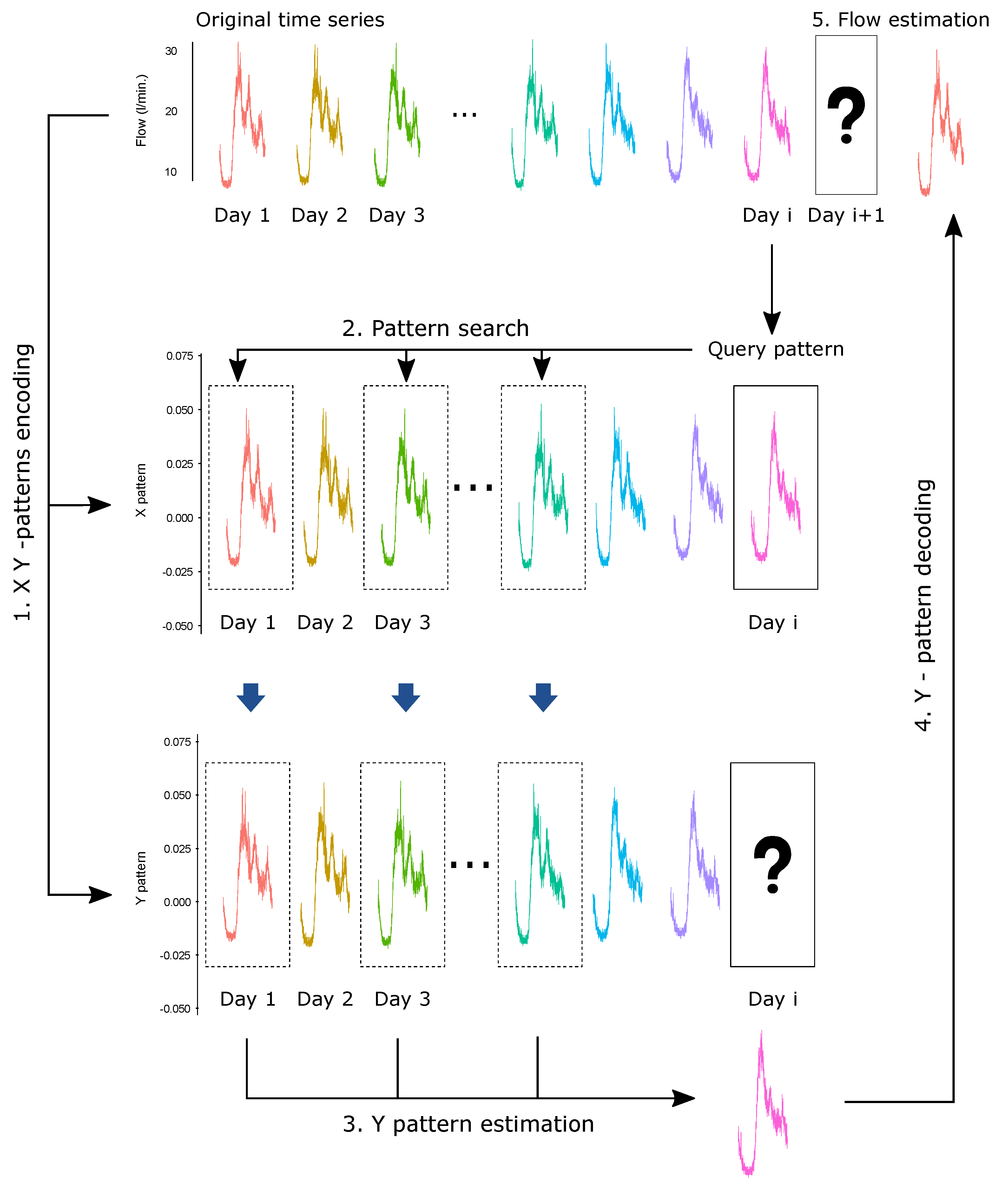
Figure 1 and Figure 2 summarize the water flow forecast procedure presented here. This procedure has the following steps:
- Assume we are at the day, and we want to make a forecast for the next () day.
- Taking as input the data in the history record, the k-nearest neighbors of the query pattern are selected among days of the same class (same day of the week) so that the next day is not an atypical one (such as holiday). In particular, given the query pattern corresponding to a weekday of class (from Monday–Sunday), we define the set:where is the weekday class of day j. Now, we compute the Euclidean distances:and then reorder the indexes j so the Euclidean distances are increasing, i.e., . Finally, we define the set of indexes of the k-nearest neighbors as:
- The estimate is calculated by:where represents the index set of the k x-patterns nearest to the query pattern that were obtained by the previous step.
- Equation (3) is used to transform and to obtain the water flow estimate .
2.6. Confidence Bounds
In order to measure the variability of the estimation due to random fluctuations, some confidence bounds must be calculated together with the estimation .
Notice that the water flow estimation for a concrete day is a linear transformation of the estimated y pattern for that day, according to Equation (3). Then, the estimation for the y pattern, for a given day i and a given hour t (within day i), is obtained by using Equation (4):
Considering that this estimation provides a mean value, for each , a given confidence interval for the mean may be obtained:
where is the confidence level, denotes the two-tailed critical value for Student’s t-distribution with degrees of freedom, and denotes the sample variance of the k values used for the calculation of :
with:
3. Results and Discussion
This section firstly describes the details about the algorithm’s application and its main parameters, as well as the goodness of fit measures considered. Secondly, the results obtained are presented and discussed.
3.1. Algorithm Application and Parameters
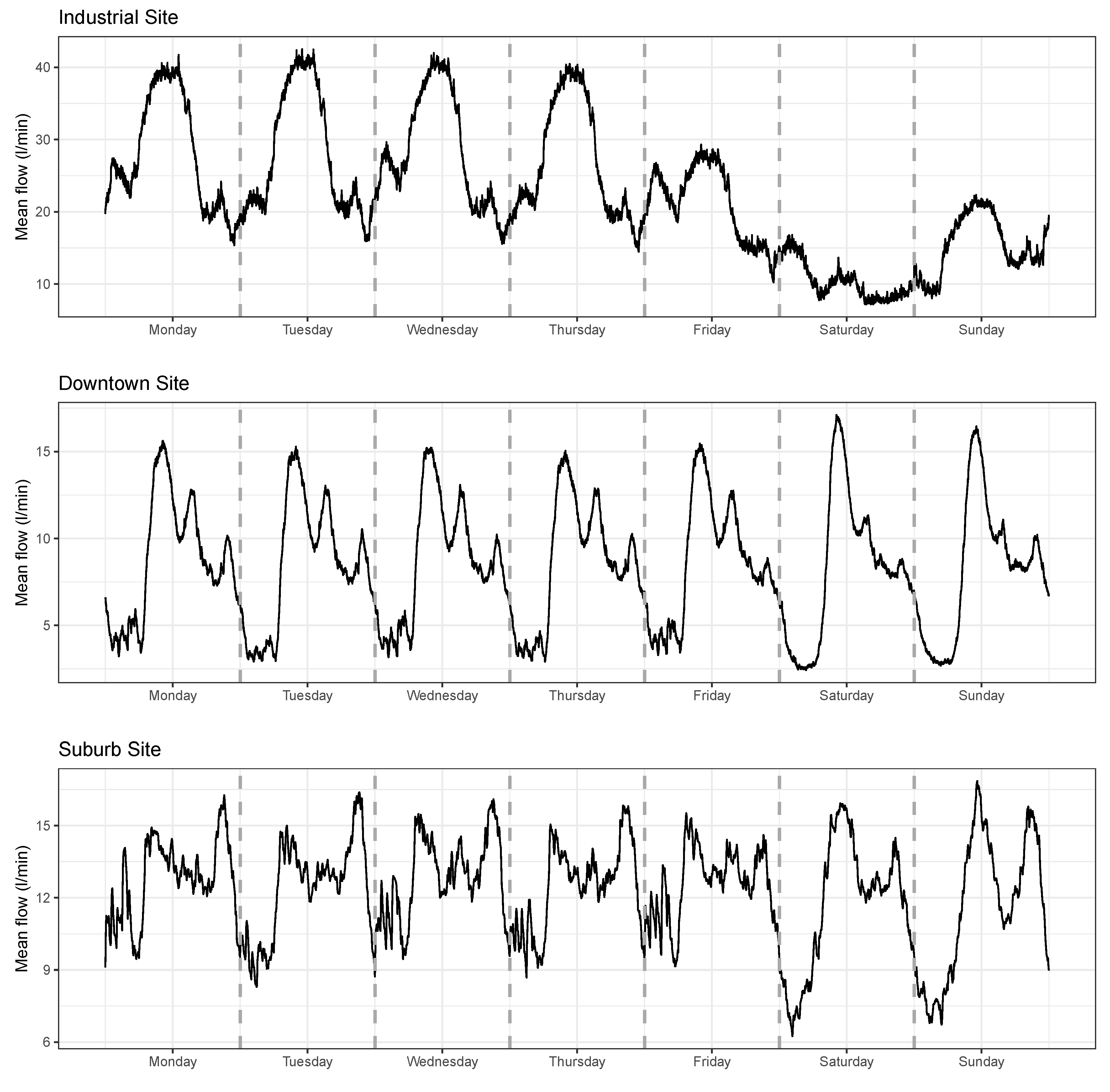
A simple exploratory analysis of the average water flows for each day of the week (see the Appendix A) allows us to infer that for the manufacturing area, four different patterns may be distinguished: Monday–Thursday, Friday, Saturday, and Sunday. On the other hand, in the downtown area, two patterns could be observed: work days (Monday–Friday) and weekends (Saturday–Sunday). Finally, for the residential area, we found far more irregular patterns. Thus, for the sake of simplicity, for the development of the algorithm, we considered the most restrictive pattern distribution (residential area) with a different pattern for each day of the week.
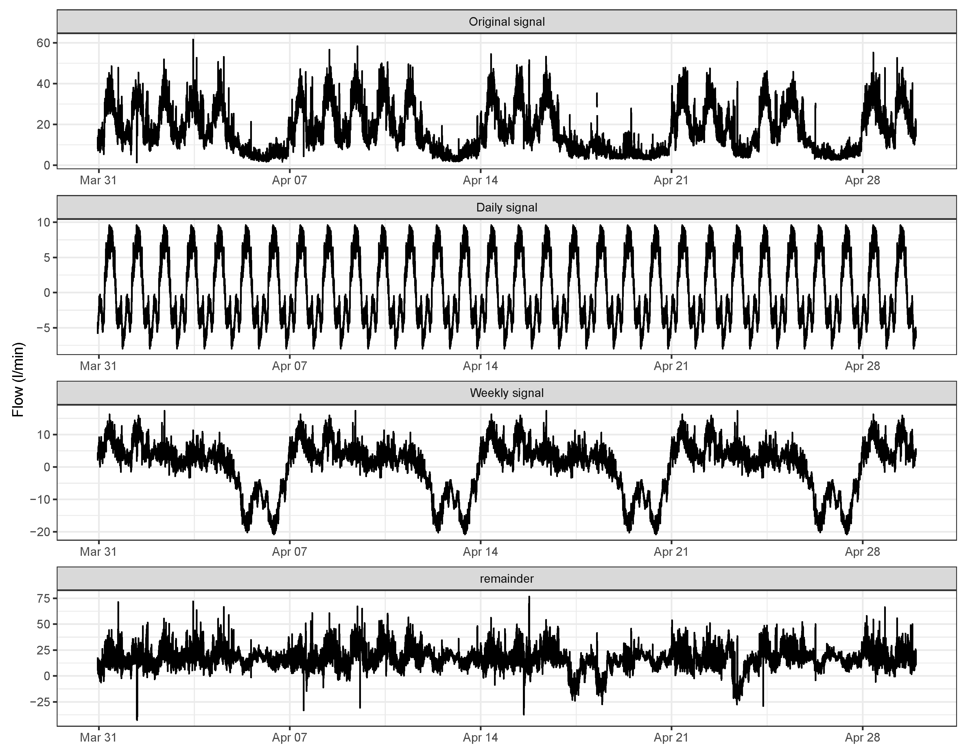
An STL decomposition for a sample month, created with R [40], is presented in Figure 3. Observe that two different seasonalities are represented in this decomposition: one with a 24-hour period and the other one with a seven-day period. While the former provides insights into the daily water flow cycle pattern, the latter does the same with respect to the weekly pattern, clearly separating the weekly pattern into two main groups: Monday–Friday and Saturday–Sunday cycles. Observe also that some oscillations are present in the remainder. These oscillations give grounds to be considered as additional information instead of simple white noise. In other words, a new STL decomposition over the signal remainder could be carried out to search for other seasonalities.
Concerning holidays, it is obvious that completely different patterns are found for such days. However, the inclusion of a holiday pattern into a model based on periodicities is not easy and cumbersome to implement since holidays’ distribution varies every year, and it is beyond the scope of this work.
The algorithm was applied in a wide range of days: all the days from 15 February 2014 to 18 September 2016. The first measurements were not used for the algorithm since they were needed as historical data for the application of the k-nearest neighbors approach. In particular, seven weeks of historical data were used due to us searching for the five nearest neighbors (see the details below). The parameters that were used for the three locations considered in the study were the next: (i) number of nearest neighbors: for all years; (ii) the threshold limits: L/min, L/min; and (iii) the confidence level for the confidence band estimation: 90% (i.e., ).
It is worth remarking about the importance of the number of neighbors parameter. On the one hand, a small value of this parameter may produce a pattern that is not representative enough for a true pattern of the forecasted day; however, on the other hand, a too high value could cause the neighbors to be “far away” from the query pattern, and the days considered for the estimation could be very different.
3.2. Goodness of Fit Measures
The Goodness of Fit (GoF) parameters that were used in the study for evaluating the approach’s performance are the following:
- MAPE (Mean Average Percentage Error): The MAPE for the estimation on day i is defined as:
- RMSE (Root Mean Squared Error): The RMSE for the estimation on day i is defined as:
- FOB (Fraction Out of Bounds): The FOB for the estimation on day i is defined as:where denotes the number of measurements on day i inside the confidence band and is the number of measurements that lie outside this confidence band.
Notice that the MAPE measure of prediction is a widely-accepted GoF indicator in this type of forecasting approach. Nevertheless, it also presents some weaknesses for those cases where measurements are close to zero (very low). Those cases may generate MAPE values greater than 100%. These situations are frequent in our study since the water flow measurements in the first hours of the day are really low in contrast to the measurements obtained in the maximum demand hours where the water flow values are much higher. Thus, the high values obtained for the MAPE parameter during the low flow times influence the daily average to result in values much greater than those that the goodness of the fit would suggest after an eye-based inspection.
RMSE is an indicator (as an absolute measure) of the deviation of the forecasted value with respect to the actual one. In other words, high values for this parameter denote a high discrepancy between prediction and observation. However, low values for this parameter do not signify a concordance between the model and measurement, especially for low water flow values.
Finally, the FOB parameter provides an overall measure of the pattern followed by a particular day of a concrete class (day of the week) in order to identify what should be considered a typical day of the class.
3.3. Results
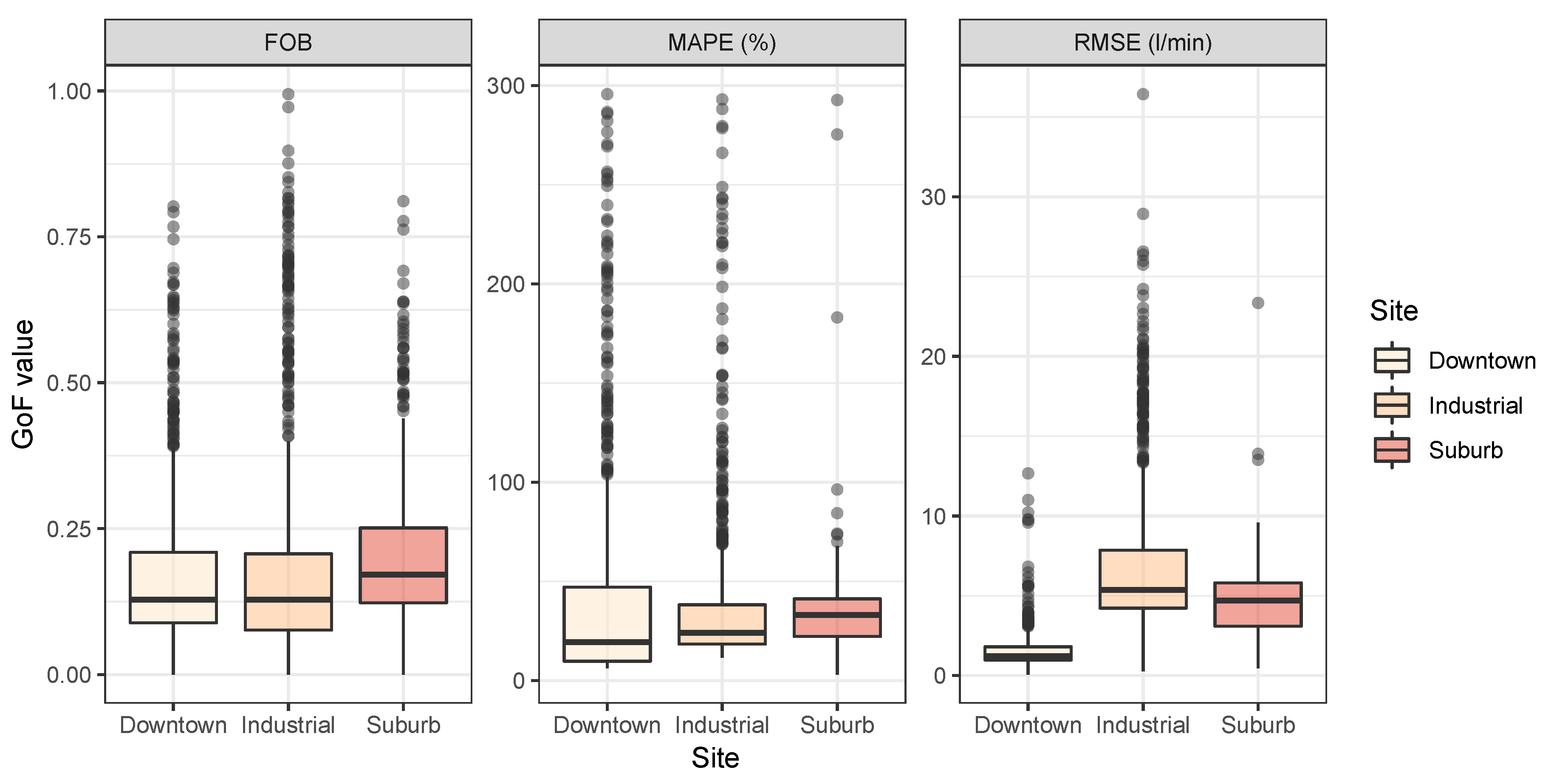
Figure 4 provides a general view of the three GoF parameters values obtained for the three locations considered in this study. We may observe that small global values were obtained for all of them. In particular, in 75% of the cases, the predictions provided values for FOB, MAPE, and RMSE lower than 0.20, 39%, and 7.86 L/min, respectively, for the manufacturing area; values lower than 0.21, 50%, and 1.80 L/min for the downtown location; and lower than 0.25, 41%, and 5.82 L/min for the residential site (see Table 3).
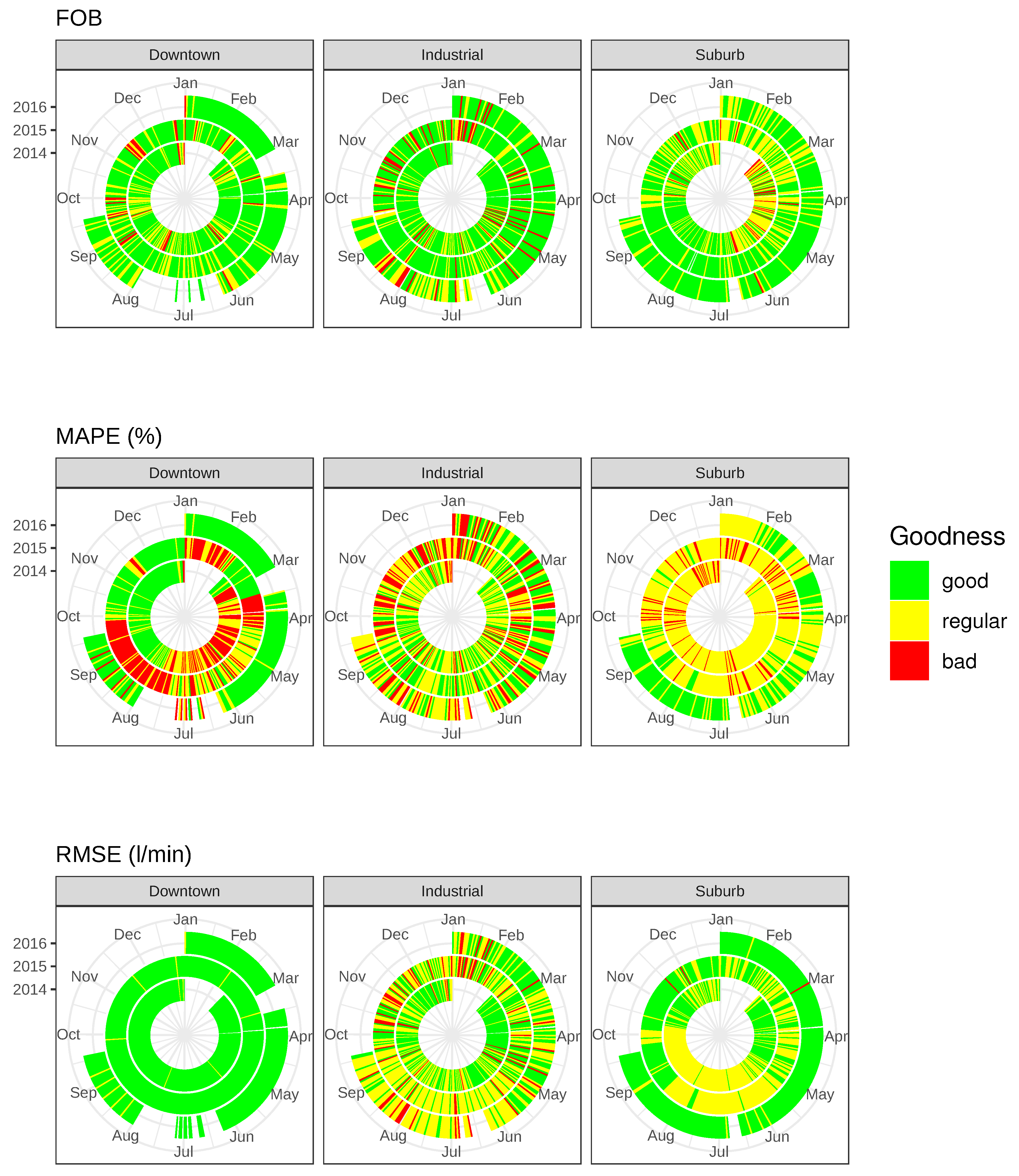
Obviously, for the cases where parameters took higher values, a deeper analysis would be needed to determine the reasons (although the errors presented small values in the overall outcomes). For this purpose, daily values were considered and represented in scatter plots, where they were classified into three different categories: good, regular, and bad (Figure 5).
3.4. Discussion
Based on the accurate results obtained in the general cases by the forecasting method applied here, we concluded that the method was suitable for water flow daily predictions. However, there were also some predictions where the values obtained were not so close to the actual measurements or that behaved worse than we expected. These concrete situations are discussed here.
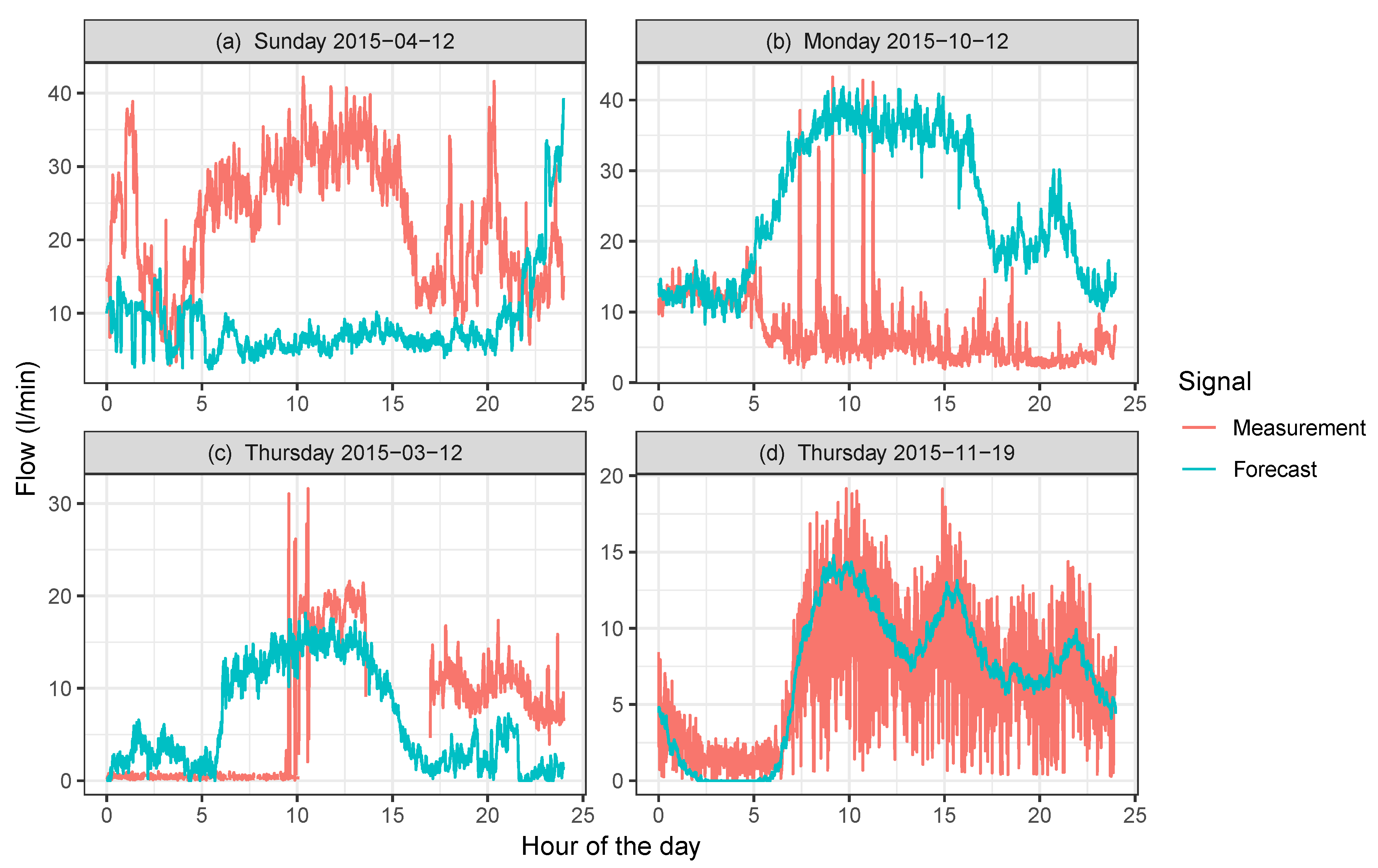
For the manufacturing location, as was expected, the days where patterns were more difficult to identify and, thus, to forecast, were Sundays (see Figure 6a), since we observed more than one pattern for this kind of day. This trend was not observed for Saturdays, which, surprisingly, followed a common pattern. Considering this situation, we used the preceding Saturday X pattern for each Sunday and searched for the k-nearest neighbors of that Saturday pattern. Due to the similarity of all the patterns, independently of the corresponding Y pattern (for the next Sunday), we observed that in many cases, the kY patterns obtained were almost random. Based on this observation, we concluded that it did not reflect the characteristic Y pattern for that day mainly due to the fact that there were several different potential Y patterns related to a given X pattern.
We also identified some problems when anomalous days were considered, e.g., holidays. Concretely, in those situations where the forecasted day, the day before or the day after, was a holiday, we observed that the forecasting approach presented some limitations for obtaining predictions. This problem was also replicated even if those days were not holidays, but an anomalous day followed one of the k-nearest neighbors considered for the X pattern for the query day. The results obtained in those cases were also distorted by that anomalous day (see Figure 6b).
Finally, and confirming our initial intuition, we observed that better measurements produced more accurate forecasts. Notice that gaps in measurements for a particular day may introduce errors and mispredictions for the algorithm (see Figure 6c), even though these gaps may be modeled as NAs (days with Non-Available data). These kinds of days should be also considered as anomalous days and flagged so that they are not included in the forecasting approach.
Regarding the downtown area, it was the location where more accurate results were obtained. This is mainly due to the high number of people that live in this area, composed of high buildings in the very center of the city considered. Note that the water flow time series for that area were regularized because of the great number of inhabitants making use of the water supply at the same time (see Appendix A Figure A1). This area provided two patterns according to the different days of the week (work days or weekends), though they looked even similar. Based on these patterns and the regularity of the signal, the results obtained denote that the forecasting procedure was even more reliable in this area. This assumption is also confirmed by the GoF parameters that provided good results in general, except for MAPE. However, as previously mentioned, this parameter was not considered because of the flaws when values close to zero were measured.
Nevertheless, for the downtown location, we also identified some anomalous situations in the predictions mainly based on the misbehavior of the time series. For example, a high frequency random component that overlapped the signal was observed 19 November 2015 (see Figure 6d). Due to this random fluctuation, the FOB value was increased to 0.51 (red flag). However, thanks to the pattern followed by the forecasted and measured values, which were similar, the original signal was well predicted. This is the reason why RMSE remained small (RMSE = 2.8 L/min) even though FOB was high.
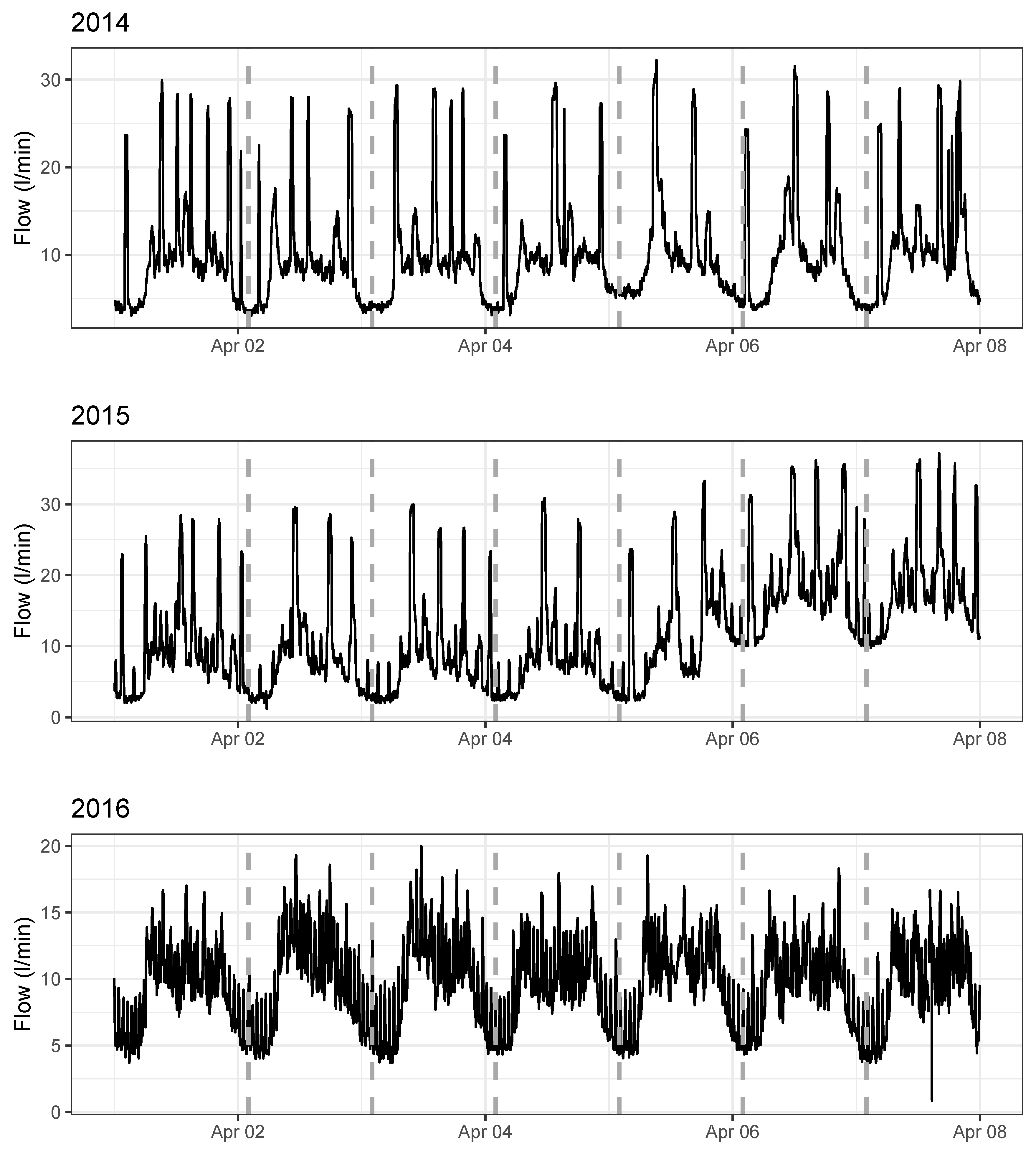
Finally, the location with the worst results for the forecasting approach was the residential area. This also confirmed our initial intuition, since: (i) the area was composed by many single-family houses with gardens; (ii) it is not a big area, and the number of concurrent water supply users (hundreds) is smaller than for the other two locations (e.g., thousand of end users in case of the downtown area). Both reasons make the consumption of each domestic user have an important weight in the signal, and so for the variance. The final result is a highly irregular time series where we may observe, for instance, that no regular patterns are followed for the same week in different years, e.g., 8–14 July for 2014, 2015, and 2016 in Figure A2. In other words, regular patterns may not be foreseen.
Although fairly good overall results were obtained for this area, the main characteristic of these signals remained highly unpredictable since their distribution were mainly random, due to sudden peaks in the water flow.
To illustrate this situation, Figure 7 represents two different days obtained by the forecasting approach: 21 and 22 October 2014, which were flagged as “green” and “red”, respectively, in the FOP plot (see Figure 5). Although these forecasts seem similar in quality, in the former, the peaks keep inside the confidence bands, whilst, in the latter, they fall outside these bands. This caused differences in the FOB for similar predictions even though the RMSE values obtained were very small for both cases (4.39 L/min and 5.08 L/min, respectively).
An important conclusion provided by the study is that there is no need for estimating the annual seasonality when the pattern similarity algorithm is used. This is due to the signal normalization procedure (obtaining the X-Y patterns), which deseaonalizes time series. Thus, this is an interesting contribution of the method.
Notice also that the pattern similarity algorithm may be easily implemented, and it is not time consuming. In particular, filtering the training data is the step that requires more time since they represent all the same days of the week in the historical record as the query day. Moreover, this filter must also consider anomalous days, i.e., neither the query day, nor the next one are holidays. This part of the algorithm is handled by database processing languages (e.g., SQL) that make it possible to accelerate the process.
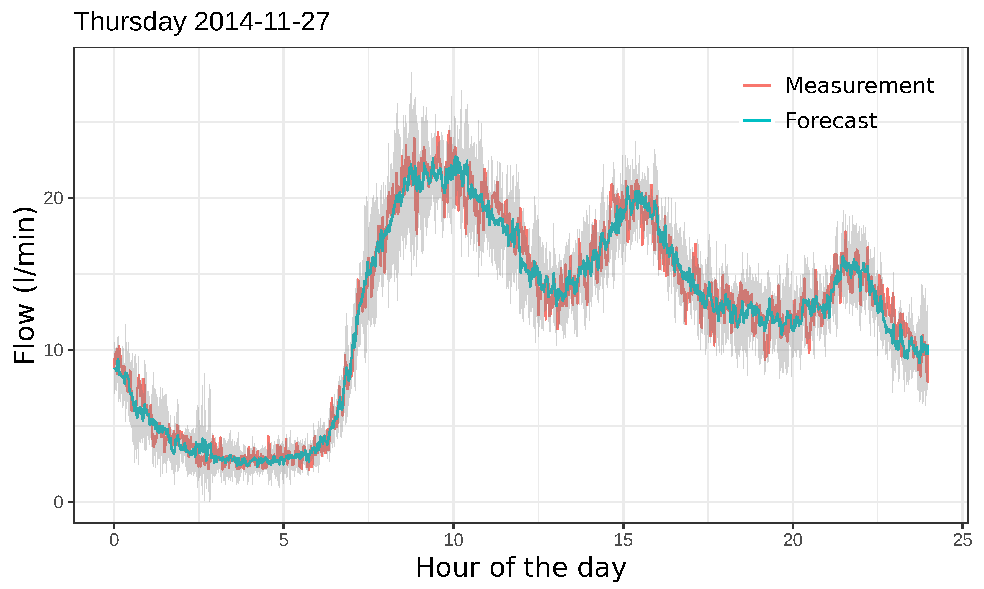
Moreover, we observed that when proper data were available (a high volume of historical data and with good quality), the forecasts obtained for the water flow of a particular day provided good predictions of the future behavior of that kind of day (see Figure 8). These good results were not altered even when the query day had small segments of missing data, since we observed that the method still behaved robustly in dealing with those anomalies. This keeps the algorithm from generating false alarms.
Finally, as the pattern-similarity method is based on forecasting the future water flow based on obtaining knowledge from past similar situations, the predictions will be even more accurate as the historical database increases in size. In other words, the more the algorithm is used in the future, the better results it will obtain.
3.5. Comparison with Previous Work
As has been stated in the Introduction, the main problem we faced was coping with a forecast horizon, which although it may seem short (in engineering terms, it was just a one-day ahead forecast), the high sampling frequency of the data (one-minute frequency) compelled us to discard some classical time series forecasting methods. For example, a direct ARIMA is absolutely unfeasible because it is well known that ARIMA models work well when the order of the auto-regressive term is not very large. Since our time series contained two principal seasonalities that were weekly and annual, one-minute frequency data would yield ARIMA orders of 10,800 (in the best case). Another approach that could overcome this difficulty while sticking to the ARIMA methodology is using Fourier regression to fit the seasonal parts of the data and to model the residuals with an ARIMA. However, the problem would be that in order to fit the annual seasonality correctly, we would need at least one year of data to be fit and then use this huge historical data to feed the ARIMA. We found this approach to be prohibitive computationally expensive.
Other classical options are neural networks. For time series forecasting, recurrent neural networks such as long-short-term memory NNs and gated recurrent units NNs, which were originally designed for sequential data (e.g., speech recognition and natural language processing), have also been used for time series forecasting. However, their use for arbitrarily large forecast horizons has been quite limited.
This section shows a comparison of the Short-Term Pattern Similarity (STPS) technique used here with other similar approaches that also allowed the same forecast horizon at a reasonable computational price. Concretely, Water Demand Forecast (-WDF) [31] and Generalized Regression Neural Network (GRNN) [6] approaches were analyzed.
As was mentioned in Section 1, -WDF relies on a moving window of three weeks used to obtain average parameters for similar days (based on the day of the week). In other words, the approach provides predictions from one, two, and three earlier weeks. In that sense, this approach has similarities to STPS in terms of the calculations of average patterns based on the same days of the week. However, unlike the -WDF approach that just considers three weeks before as the available window, the method presented here uses the k nearest neighbors of the query pattern obtained from the data in the historical record.
On the other hand, the GRNN approach has similarities to STPS with respect to data preprocessing [36] since: firstly, it is also based on the X-Y pattern similarity that allows removing seasonal components; secondly, it also applies the nearest k-neighbors technique. However, it also presents differences with respect to our approach, namely it uses a neural network with an intermediate layer with a single neuron and weights based on radial basis functions. This approach also provides an average of certain Y patterns as the results, but with weights provided by a Gaussian kernel [36].
Feed-forward neural networks or long-short-term memory networks are other examples of forecasting approaches based on ANNs that have been recently developed. However, these approaches could not be compared with that presented here since 24 h is commonly claimed to be a short-term period for a forecast, whilst the number of predicted values for high frequency data series was really high (1440). Thus, the application of an ANN approach in our study would require a 1440-node output layer and hidden and input layers with also a high number of nodes. This kind of network would require a huge amount of training data.
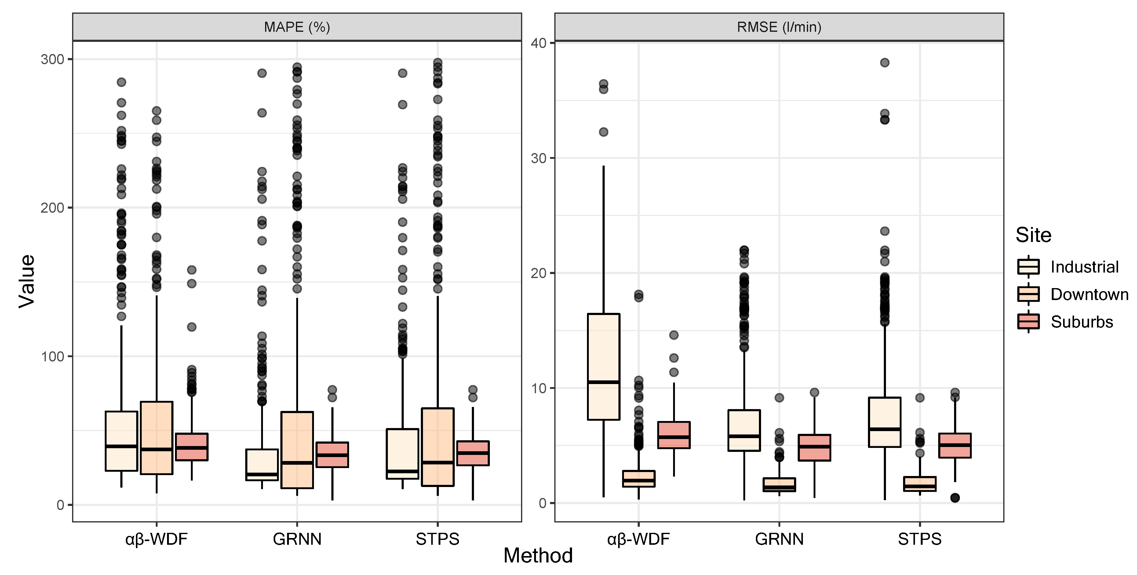
For performing this comparison with the related approaches, all the data from 2015 were taken into account, since the historical record was complete for that year. Then, MAPE and RMSE error parameters introduced in [31] were calculated. The reason for using these two values is that the MAPE value may become really high due to: (i) each day having a high number of predicted values (1400) and (ii) the water demand being almost null in some periods of the day. Thus, the RMSE was also used since it may provide adequate values to determine the prediction accuracy in such situations.
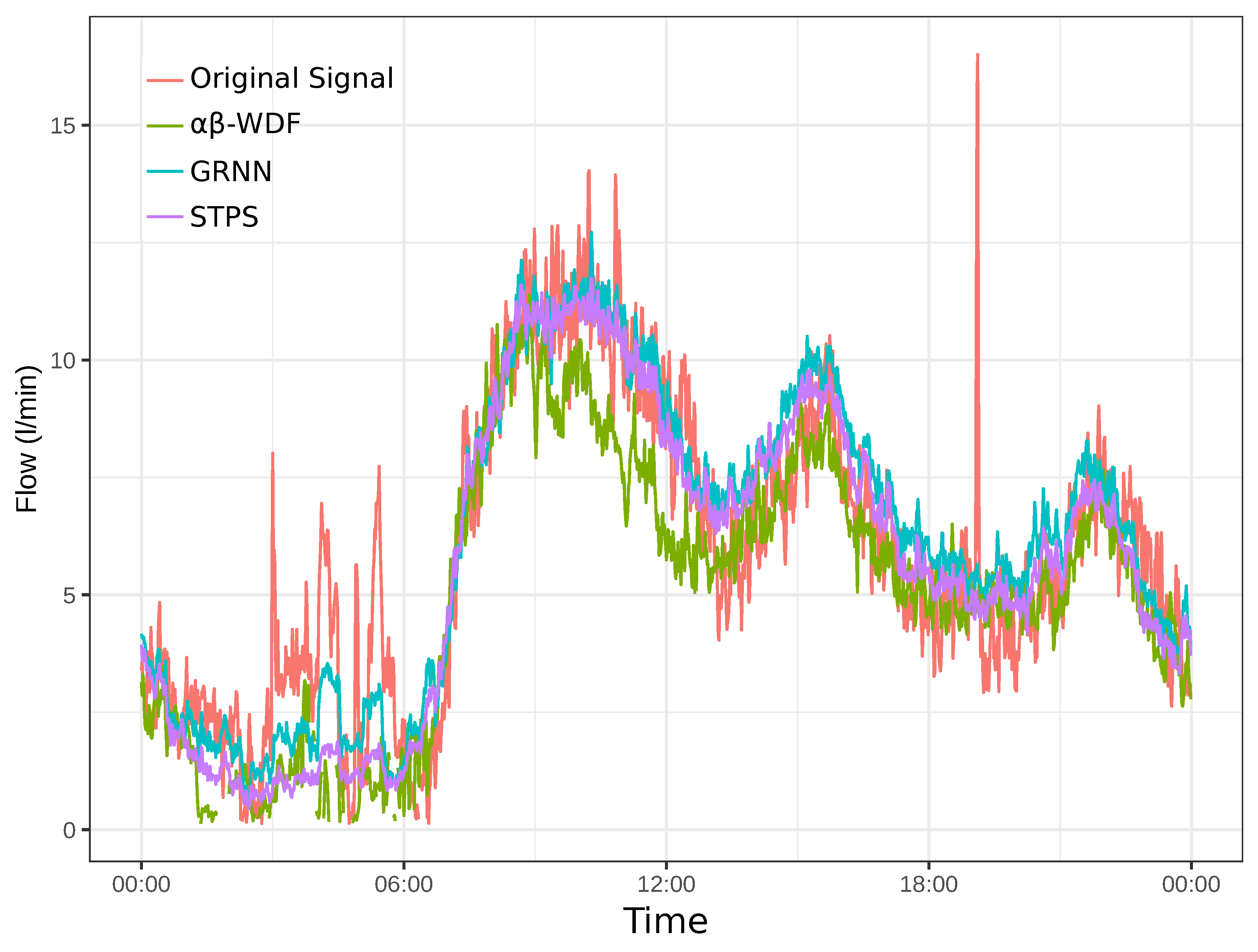
Finally, Figure 9 shows a comparison among the measured and predicted values for the different approaches considered here. These values were obtained for a randomly picked day (1 June 2015) and for the downtown area. Similarly, Figure 10 compares the MAPE and RMSE values obtained for the three scenarios and for each approach. Note that those approaches that presented better results were STPS and GRNN, whilst -WDF provided poorer predictions for the three locations.
4. Conclusions and Future Work
As has been shown in the study, an accurate forecast of time series relies heavily on the regularity of the signals. The more regular a signal is, the easier it will be to predict. Flow measurements in water pipes are an example of time series that, in principle, show regular patterns because they depend on human activity, which is highly regular. However, this regularity is formed by the overlapping of several periodic signals of different periods; most importantly, the daily, weekly, and annual periods.
Classical statistical tools for time series analysis have been widely used for forecasting this class of time series. However, as has been mentioned in the paper, the inclusion of several seasonalities is quite cumbersome, and the fitting horizons are not very large.
Pattern similarity techniques, such as the one presented here, cope with these two difficulties at the same time; they remove the need to determine the annual seasonality by constructing the X and Y patterns in which the series has been normalized, and at the same time, since the signal segments considered encompassed a full day, the forecast horizon was 24 h.
Although the results obtained in the work were quite convincing and promising, there were some drawbacks that we would like to handle in the future. Avoiding the problems with anomalous days, namely holidays and abnormal days, is the first issue to be considered. Holidays can be handled as long as the historical record contains enough data to construct training sets from which to obtain the nearest neighbors. In the case of abnormal days, they could be flagged as anomalous, once they have been identified, and they may be removed from the possible training subsets in the forecasting of other days.
For those locations where there is not regularity in the signal (e.g., the residential area in this study), the approach could also consider shorter prediction windows, e.g., 4–6 h. However, this hypothesis still needs further work in order to be deeply analyzed.
Moreover, it is noteworthy that the method proposed here allows us to determine in advance what a standard day would look like, given the information of the current day. This would be very helpful for detecting anomalies, such as water leaks, in the water distribution network. Future work would be to couple the water flow time series with the water pressure time series in order to design a water leak detection algorithm, which, combined with the high frequency data available, would allow us to detect and repair water leaks swiftly. This, in a country like Spain, where the concern for the use and saving of water is increasing and where the problems derived from the lack of water and droughts are seemingly going to be aggravated in the coming years, would represent a remarkable advance.
Finally, we plan to apply the approach to other cities where collaborations have been maintained based on the project that this research is framed on, e.g., Leeuwarden (Holland), Reading (United Kingdom), or Lille (France).
Author Contributions
Conceptualization, J.C.P., F.S.F., and J.M.C.; data curation, R.B. and C.O.-C.; formal analysis, R.B. and A.R.-L.; research, R.B., A.R.-L., J.C.P., and J.M.C.; methodology, R.B. and J.C.P.; project administration, F.S.F. and J.C.P.; resources, R.B. and A.R.-L.; software, F.S.F., J.C.P., and J.M.C.; supervision, R.B., F.S.F., and J.C.P.; validation, R.B., C.O.-C., and A.R.-L.; visualization, R.B. and C.O.-C.; writing, original draft, R.B., A.R.-L., and J.C.P.; writing, review and editing, A.R.-L., F.S.F., and J.M.C.
Funding
The authors wish to acknowledge the collaborative funding support from (i) Consejería de Economía e Infraestructuras (Junta de Extremadura, Spain), European Regional Development Fund (ERDF), GR18112, IB16055, and IB18034 projects; (ii) RTI2018-098652-B-I00 project (MCIU/AEI/FEDER, UE).
Conflicts of Interest
The authors declare no conflict of interest.
Appendix A
This section presents some supplementary information related to the study presented.
Figure A1.
Mean flow vs. day of the week. For each of the three sites, the average for each minute of each weekday is plotted.
Figure A1.
Mean flow vs. day of the week. For each of the three sites, the average for each minute of each weekday is plotted.

Figure A2.
Comparison of the same week of April over the three sampled years (2014, 2015, and 2016) for the suburb site.
Figure A2.
Comparison of the same week of April over the three sampled years (2014, 2015, and 2016) for the suburb site.

References
- W-SMART Team. Background and FP7 Goals. Available online: https://sw4eu.com/background-fp7-goals/ (accessed on 14 March 2018).
- Alliance for Water Efficiency. Water Loss Control—Efficiency in the Water Utility Sector. Available online: http://www.allianceforwaterefficiency.org/Water_Loss_Control_Introduction.aspx (accessed on 14 March 2018).
- Center for Neighborhood Technology (CNT). The Case for Fixing the Leaks: Protecting People and Saving Water while Supporting Economic Growth in the Great Lakes Region (2013). 2013. Available online: https://www.cnt.org/publications/the-case-for-fixing-the-leaks-protecting-people-and-saving-water-while-supporting (accessed on 14 March 2018).
- Dudek, G. Pattern similarity-based methods for short-term load forecasting—Part 1: Principles. Appl. Soft Comput. 2015, 37, 277–287. [Google Scholar] [CrossRef]
- Dudek, G. Pattern similarity-based methods for short-term load forecasting—Part 2: Models. Appl. Soft Comput. 2015, 36, 422–441. [Google Scholar] [CrossRef]
- Dudek, G. Pattern-based local linear regression models for short-term load forecasting. Electr. Power Syst. Res. 2016, 130, 139–147. [Google Scholar] [CrossRef]
- Meliá, S.; Gómez, J.; Pérez, S.; Díaz, O. A Model-Driven Development for GWT-Based Rich Internet Applications with OOH4RIA. In Proceedings of the Eighth International Conference on Web Engineering, ICWE 2008, Yorktown Heights, NY, USA, 14–18 July 2008; pp. 13–23. [Google Scholar] [CrossRef]
- Martínez, Y.; Cachero, C.; Meliá, S. MDD vs. traditional software development: A practitioner’s subjective perspective. Inf. Softw. Technol. 2013, 55, 189–200. [Google Scholar] [CrossRef]
- Donkor, E.A.; Mazzuchi, T.A.; Soyer, R.; Roberson, J.A. Urban Water Demand Forecasting: Review of Methods and Models. J. Water Resour. Plan. Manag. 2014, 140, 146–159. [Google Scholar] [CrossRef]
- Caiado, J. Performance of Combined Double Seasonal Univariate Time Series Models for Forecasting Water Demand. J. Hydrol. Eng. 2010, 15, 215–222. [Google Scholar] [CrossRef] [Green Version]
- Herrera, M.; Torgo, L.; Izquierdo, J.; Pérez-García, R. Predictive models for forecasting hourly urban water demand. J. Hydrol. 2010, 387, 141–150. [Google Scholar] [CrossRef]
- Adamowski, J.; Karapataki, C. Comparison of Multivariate Regression and Artificial Neural Networks for Peak Urban Water-Demand Forecasting: Evaluation of Different ANN Learning Algorithms. J. Hydrol. Eng. 2010, 15, 729–743. [Google Scholar] [CrossRef] [Green Version]
- Odan, F.K.; Reis, L.F.R. Hybrid water demand forecasting model associating artificial neural network with Fourier series. J. Water Resour. Plan. Manag. 2012, 138, 245–256. [Google Scholar] [CrossRef]
- Adamowski, J.; Fung Chan, H.; Prasher, S.O.; Ozga-Zielinski, B.; Sliusarieva, A. Comparison of multiple linear and nonlinear regression, autoregressive integrated moving average, artificial neural network, and wavelet artificial neural network methods for urban water demand forecasting in Montreal, Canada. Water Resour. Res. 2012, 48. [Google Scholar] [CrossRef]
- Bakker, M.; Vreeburg, J.; van Schagen, K.; Rietveld, L. A fully adaptive forecasting model for short-term drinking water demand. Environ. Model. Softw. 2013, 48, 141–151. [Google Scholar] [CrossRef]
- Romano, M.; Kapelan, Z. Adaptive water demand forecasting for near real-time management of smart water distribution systems. Environ. Model. Softw. 2014, 60, 265–276. [Google Scholar] [CrossRef] [Green Version]
- Kim, J.Y.; Jung, J.H.; Yoon, Y.H.; An, J.S.; Kim, W.J.; Oh, H.J. Development of Demand Prediction Simulator Based on Multiple Water Resources. APCBEE Procedia 2014, 10, 224–228. [Google Scholar] [CrossRef] [Green Version]
- Ji, G.; Wang, J.; Ge, Y.; Liu, H. Urban water demand forecasting by LS-SVM with tuning based on elitist teaching-learning-based optimization. In Proceedings of the 26th Chinese Control and Decision Conference (2014 CCDC), Changsha, China, 31 May–2 June 2014; pp. 3997–4002. [Google Scholar]
- Sampathirao, A.K.; Grosso, J.M.; Sopasakis, P.; Ocampo-Martinez, C.; Bemporad, A.; Puig, V. Water demand forecasting for the optimal operation of large-scale drinking water networks: The Barcelona Case Study. IFAC Proc. Vol. 2014, 47, 10457–10462. [Google Scholar] [CrossRef]
- Candelieri, A.; Archetti, F. Identifying Typical Urban Water Demand Patterns for a Reliable Short-term Forecasting—The Icewater Project Approach. Procedia Eng. 2014, 89, 1004–1012. [Google Scholar] [CrossRef]
- Hutton, C.J.; Kapelan, Z. A probabilistic methodology for quantifying, diagnosing and reducing model structural and predictive errors in short term water demand forecasting. Environ. Model. Softw. 2015, 66, 87–97. [Google Scholar] [CrossRef]
- Bai, Y.; Wang, P.; Li, C.; Xie, J.; Wang, Y. Dynamic Forecast of Daily Urban Water Consumption Using a Variable-Structure Support Vector Regression Model. J. Water Resour. Plan. Manag. 2015, 141, 04014058. [Google Scholar] [CrossRef]
- Wu, M.C.; Lin, G.F. An Hourly Streamflow Forecasting Model Coupled with an Enforced Learning Strategy. Water 2015, 7, 5876–5895. [Google Scholar] [CrossRef] [Green Version]
- Candelieri, A.; Soldi, D.; Archetti, F. Short-term forecasting of hourly water consumption by using automatic metering readers data. Procedia Eng. 2015, 119, 844–853. [Google Scholar] [CrossRef]
- Arandia, E.; Ba, A.; Eck, B.; McKenna, S. Tailoring Seasonal Time Series Models to Forecast Short-Term Water Demand. J. Water Resour. Plan. Manag. 2016, 142, 04015067. [Google Scholar] [CrossRef]
- Sebri, M. Forecasting urban water demand: A meta-regression analysis. J. Environ. Manag. 2016, 183, 777–785. [Google Scholar] [CrossRef] [PubMed]
- Shabani, S.; Yousefi, P.; Adamowski, J.; Naser, G. Intelligent Soft Computing Models in Water Demand Forecasting. In Water Stress in Plants; InTech: London, UK, 2016. [Google Scholar] [Green Version]
- Anele, A.; Hamam, Y.; Abu-Mahfouz, A.; Todini, E. Overview, comparative assessment and recommendations of forecasting models for short-term water demand prediction. Water 2017, 9, 887. [Google Scholar] [CrossRef]
- Gagliardi, F.; Alvisi, S.; Kapelan, Z.; Franchini, M. A probabilistic short-term water demand forecasting model based on the Markov Chain. Water 2017, 9, 507. [Google Scholar] [CrossRef]
- Candelieri, A. Clustering and Support Vector Regression for Water Demand Forecasting and Anomaly Detection. Water 2017, 9, 224. [Google Scholar] [CrossRef]
- Pacchin, E.; Alvisi, S.; Franchini, M. A short-term water demand forecasting model using a moving window on previously observed data. Water 2017, 9, 172. [Google Scholar] [CrossRef]
- Brentan, B.M.; Luvizotto, E., Jr.; Herrera, M.; Izquierdo, J.; Pérez-García, R. Hybrid regression model for near real-time urban water demand forecasting. J. Comput. Appl. Math. 2017, 309, 532–541. [Google Scholar] [CrossRef]
- Alvisi, S.; Franchini, M. Assessment of predictive uncertainty within the framework of water demand forecasting using the Model Conditional Processor (MCP). Urban Water J. 2017, 14, 1–10. [Google Scholar] [CrossRef]
- Anele, A.O.; Todini, E.; Hamam, Y.; Abu-Mahfouz, A.M. Predictive uncertainty estimation in water demand forecasting using the model conditional processor. Water 2018, 10, 475. [Google Scholar] [CrossRef]
- Navarrete-López, C.; Herrera, M.; Brentan, B.; Luvizotto, E.; Izquierdo, J. Enhanced Water Demand Analysis via Symbolic Approximation within an Epidemiology-Based Forecasting Framework. Water 2019, 11, 246. [Google Scholar] [CrossRef]
- Dudek, G. Neural networks for pattern-based short-term load forecasting: A comparative study. Neurocomputing 2016, 205, 64–74. [Google Scholar] [CrossRef]
- Specht, D.F. A general regression neural network. IEEE Trans. Neural Netw. 1991, 2, 568–576. [Google Scholar] [CrossRef] [PubMed]
- Agua, A. Propuesta Algoritmo de Estimación de Caudales; Technical Report; Acciona Agua: Madrid, Spain, 2016. [Google Scholar]
- Cleveland, R.B.; Cleveland, W.S.; McRae, J.E.; Terpenning, I. STL: A seasonal-trend decomposition procedure based on loess. J. Off. Stat. 1990, 6, 3–73. [Google Scholar]
- R Core Team. R: A Language and Environment for Statistical Computing; R Foundation for Statistical Computing: Vienna, Austria, 2016. [Google Scholar]
Figure 1.
Scheme of the pattern-similarity method.

Figure 2.
Flow-chart of the algorithm applied.

Figure 3.
One-month STL(seasonal trend decomposition based on Locally Estimated Scatterplot Smoothing (LOESS)) decomposition. The different plots show, from top to bottom, the original signal (raw data), the seasonal (both daily and weekly), and the remainder components.
Figure 3.
One-month STL(seasonal trend decomposition based on Locally Estimated Scatterplot Smoothing (LOESS)) decomposition. The different plots show, from top to bottom, the original signal (raw data), the seasonal (both daily and weekly), and the remainder components.

Figure 4.
Distributions of the values of the goodness of fit parameters FOB, MAPE, and RMSE at the three site (downtown, industrial site, and suburb) over the entire period of study, 2014–2016.
Figure 4.
Distributions of the values of the goodness of fit parameters FOB, MAPE, and RMSE at the three site (downtown, industrial site, and suburb) over the entire period of study, 2014–2016.

Figure 5.
Daily values of the FOB (top plot), MAPE, and RMSE (middle plot) at the three sites from 2014 (inner circles) to 2016 (outer circles). The values are gathered into three different categories: good (green shading), regular (yellow shading), and bad (red shading), depending on the values taken by the GoF measure. For FOB, the categories are respectively defined by the intervals , , and ; for MAPE, the categories are defined by , , and ; and for RMSE, the intervals defining the categories are (units in L/min) , , and .

Figure 6.
Examples of troublesome signals. In (a), the forecasted day was on Sunday, 12 April 2015, for the industrial site. For this site, Saturdays were very similar, and Sundays differed depending on other factors (e.g., the time of the year). This led to an improper forecasting since the k Saturdays closest to 11 April 2015 were not followed by Sundays similar to the forecasted day. In (b), the forecast was for Monday, 2 November 2015, for the industrial site. This day was a holiday. In this case, since the day before was a Sunday, the predicted values were the average of k normal Mondays, which obviously had a very different behavior. In (c), the effect of missing data in both the prediction and query days is visible. When there were missing data in the query day, since only the remaining data were considered, the neighbors were improperly obtained, and thus, one might obtain a misleading neighbor, which would yield erroneous forecasting results. When data are missing for the forecasting day, there cannot be accurate predictions. In (d), the forecasting for the downtown site on 19 November 2015 is depicted. The water flow measurements showed a very large random component, which greatly increased its variance. However, the general pattern of the series was well predicted.

Figure 7.
Comparison of two forecasts for the suburban site. The first one (left plot) was flagged as “green” in the FOB plot (FOB = 0.08), while the second (right plot) was flagged as “red” (FOB = 0.51). The grey band represents the 10% pointwise confidence bands.
Figure 7.
Comparison of two forecasts for the suburban site. The first one (left plot) was flagged as “green” in the FOB plot (FOB = 0.08), while the second (right plot) was flagged as “red” (FOB = 0.51). The grey band represents the 10% pointwise confidence bands.

Figure 8.
Example of a good forecast for the downtown site. The grey band represents the 10% pointwise confidence band.
Figure 8.
Example of a good forecast for the downtown site. The grey band represents the 10% pointwise confidence band.

Figure 9.
Forecasting for the downtown site for Wednesday, 1 June 2015. The red line denotes the measured values, the green line the predicted values by the -WDF (Water Demand Forecast) approach, the blue line the prediction of GRNN (Generalized Regression Neural Network), and the violet line the predicted values by our approach (STPS, Short-Term Pattern Similarity).

Figure 10.
Boxplot of the goodness of fit parameter comparison among the -WDF, GRNN, and STPS approaches for the three measured sites.
Figure 10.
Boxplot of the goodness of fit parameter comparison among the -WDF, GRNN, and STPS approaches for the three measured sites.


Table 1.
Structure of the raw data from the industrial site (first six measurements).
| Industrial Site | |||
|---|---|---|---|
| timestamp | average | maximum | minimum |
| 2014-01-01 00:00:00+01 | 3.278 | 4.031 | 2.919 |
| 2014-01-01 00:01:00+01 | 3.591 | 5.064 | 3.049 |
| 2014-01-01 00:02:00+01 | 4.875 | 5.352 | 4.518 |
| 2014-01-01 00:03:00+01 | 4.263 | 5.074 | 3.475 |
| 2014-01-01 00:04:00+01 | 3.966 | 5.004 | 3.406 |
| 2014-01-01 00:05:00+01 | 3.771 | 4.031 | 3.188 |
| ⋯ | ⋯ | ⋯ | ⋯ |
Table 2.
Structure of the preprocessed data from the industrial site (first six measurements).
| Industrial Site | ||
|---|---|---|
| average | time | weekday |
| 3.278 | 2014-01-0100:00:00 | Wednesday |
| 3.591 | 2014-01-01 00:01:00 | Wednesday |
| 4.875 | 2014-01-01 00:02:00 | Wednesday |
| 4.263 | 2014-01-01 00:03:00 | Wednesday |
| 3.966 | 2014-01-01 00:04:00 | Wednesday |
| 3.771 | 2014-01-01 00:05:00 | Wednesday |
| ⋯ | ⋯ | ⋯ |
Table 3.
The 75% quantile for the Goodness of Fit (GoF) parameters at the three sites over the entire period. FOB, Fraction Out of Bounds.
Table 3.
The 75% quantile for the Goodness of Fit (GoF) parameters at the three sites over the entire period. FOB, Fraction Out of Bounds.
| Site | GoF | ||
|---|---|---|---|
| FOB (Ratio) | MAPE (%) | RMSE (L/min) | |
| Industrial | 0.20 | 39 | 7.86 |
| Downtown | 0.21 | 50 | 1.80 |
| Suburbs | 0.25 | 41 | 5.82 |
© 2019 by the authors. Licensee MDPI, Basel, Switzerland. This article is an open access article distributed under the terms and conditions of the Creative Commons Attribution (CC BY) license (http://creativecommons.org/licenses/by/4.0/).
Share and Cite
MDPI and ACS Style
Benítez, R.; Ortiz-Caraballo, C.; Preciado, J.C.; Conejero, J.M.; Sánchez Figueroa, F.; Rubio-Largo, A. A Short-Term Data Based Water Consumption Prediction Approach. Energies 2019, 12, 2359. https://doi.org/10.3390/en12122359
AMA Style
Benítez R, Ortiz-Caraballo C, Preciado JC, Conejero JM, Sánchez Figueroa F, Rubio-Largo A. A Short-Term Data Based Water Consumption Prediction Approach. Energies. 2019; 12(12):2359. https://doi.org/10.3390/en12122359
Chicago/Turabian StyleBenítez, Rafael, Carmen Ortiz-Caraballo, Juan Carlos Preciado, José M. Conejero, Fernando Sánchez Figueroa, and Alvaro Rubio-Largo. 2019. "A Short-Term Data Based Water Consumption Prediction Approach" Energies 12, no. 12: 2359. https://doi.org/10.3390/en12122359
Note that from the first issue of 2016, this journal uses article numbers instead of page numbers. See further details here.