Fault-Tolerant Control for Actuator Faults of Wind Energy Conversion System

Abstract

The problem of robust fault-tolerant control for actuators of nonlinear systems with uncertain parameters is studied in this paper. Takagi–Sugeno (T-S) fuzzy model is used to describe the wind energy conversion system (WECS). Fuzzy dedicated observer (FDO) and fuzzy proportional integral observer (FPIO) are established to reconstruct the system state and actuator fault, respectively. Fuzzy Robust Scheduling Fault-Tolerant Controller (FRSFTC) is designed by parallel distributed compensation (PDC) method, so as to realize the purpose of active fault tolerance for actuator faults and ensure the robust stability of the system. The stability of the closed-loop system is proved by Taylor series, Lyapunov function, and Linear Matrix Inequalities (LMIs). Finally, the simulation results verify that the proposed method is feasible and effective applied to WECS with doubly fed induction generators (DFIG).

1. Introduction

With the development of science and technology, many high-level comprehensive complex nonlinear systems have been applied at a large scale. It is becoming increasingly important to have certain fault tolerance for the control system to ensure the safety and reliability of the control system. As an important green energy, wind energy development and use has become a focus in the global energy field [1,2,3,4]. The wind energy conversion system (WECS) is a typical large and complex nonlinear system with random and intermittent wind force. A WECS fault can be categorized into three types—transmission system fault, converter fault, and power grid fault—among which the transmission system, because of its structural characteristics, produces tooth surface wear, fatigue erosion, broken teeth and bearing resistance, planetary wheel cracking, and other problems [5,6]. Therefore, the transmission system has the highest probability of failure, which has the greatest impact on the WECS performance. To ensure the safe and efficient operation of wind turbines, fault-tolerant control (FTC) becomes a hotspot of research regarding WECS.

Currently, in the fault-tolerant control of WECS, the H∞ infinity fault-tolerant control method for WECS was studied based on the random piece wise affine (PWA) model. The modeling and fault-tolerant control of WECS under random wind load were solved [7]. The research illustrates that this method has better fault tolerance for sensor and actuator gain faults in WECS; the angle estimation of the pitch system is carried out by Kalman filter, to detect the fault of the blade pitch system and achieve satisfactory detection results [8]. The results show that this method can improve the efficiency of wind energy capture; on the basis of the adaptive fault observer, a state feedback fault-tolerant controller was designed to ensure the good performance of the system in normal operation in case of failure [9].

The essence of T-S fuzzy model is to use if-then fuzzy inference rules to describe the nonlinear system. Each inference rule stands for the dynamics of the local regional linear model. Using the membership function to connect the local linear models to obtain the overall fuzzy linear model, and then achieve the purpose of system modeling. In recent years, T-S fuzzy model has been widely used in controller design and system performance analysis of uncertain nonlinear systems due to its advantages such as simple structure and strong approximation, which enables it to approximate almost any complex nonlinear system [10,11,12,13,14,15]. A reliable hybrid H∞/passive control problem for T-S fuzzy time-delay systems was studied based on the semi-Markov jump model (SMJM) [16]; T-S model was used to describe the offshore wind power system, and proposing an active fault-tolerant tracking control method for sensor faults [17]; T-S modeling of doubly fed wind power system was also carried out [18,19]. For the actuator or sensor faults of the system, fault-tolerant controllers were established based on fuzzy synovial observer and fuzzy observer, respectively. However, the robust stability of the system cannot be fully guaranteed because the uncertainty generated by the system were not taken into account in the literature.

In this study, T-S fuzzy model is used to describe the WECS, and the unmeasurable state variables and uncertainties in the system are taken into account. Based on the T-S fuzzy model, the system state is estimated effectively by fuzzy dedicated observer (FDO). Fuzzy proportional integral observer (FPIO) is designed for system actuator fault to realize accurate reconstruction of fault signal. According to the estimated fault information, a robust scheduling fault-tolerant controller is designed by using parallel distributed compensation (PDC) method to realize real-time compensation for actuator faults of uncertain nonlinear systems. Taylor series and Lyapunov stability theory are used to prove the necessary and sufficient conditions to keep the closed-loop stability of the system. Finally, the feedback gain matrices are obtained via addressing Linear Matrix Inequalities (LMIs). Simulation results further verify the proposed control strategy is reliability and effectiveness applied to WECS.

2. Problem Description

2.1. Design of TS Fuzzy Model

A series of fuzzy rules are established for the nonlinear system with uncertainty. Each rule represents one of the subsystems, so the T-S model structure of uncertain parameters fuzzy system Equation (1) is described as follows:

$R^i$: If $z_1(t)\mathrm{is}{F}_1^i\mathrm{and}{z}_2(t)\mathrm{is}{F}_2^i\dots \mathrm{and}{z}_k(t)\mathrm{is}{F}_k^i$, then

$$\begin{array}{l}\dot{x}(t)=(A_i+\Delta A_i)x(t)+(B_i+\Delta B_i)u(t)\\ y(t)=C_{i}x(t)\hspace{1em}\hspace{1em}\hspace{1em}\hspace{1em}\hspace{1em}\hspace{1em}\hspace{1em}\hspace{1em}\hspace{1em}i=1,2\dots r\end{array}$$

(1)

where $R^i$ is the $i\mathrm{th}$ fuzzy inference rule, $z(t)={\left[z_1(t)z_2(t)\dots z_k(t)\right]}^T$ denotes the premise variables, $F_j^i$ is the fuzzy sets; $i=1,2,\dots ,r$ is the number of system fuzzy inference rules, $j=1,2\dots k$, $x(t)\in R^n$ is the state of the system, $u(t)\in R^m$ represents the control input, $y(t)\in R^p$ is the system output; $A_i\in R^{n\times n}$, $B_i\in R^{n\times m}$ and $C_i\in R^{p\times n}$ are the parameter matrices of the system, $\Delta A_i$ and $\Delta B_i$ are the uncertain real value matrices. It is assumed that the uncertainty norm of the system is bounded. The entire equation of state of the whole fuzzy T-S system Equation (2) can be obtained after inverse fuzzification:

$$\begin{array}{l}\dot{x}(t)={\displaystyle \sum _{i=1}^r{u}_i(z(t))}\left[(A_i+\Delta A_i)x(t)+(B_i+\Delta B_i)u(t)\right]\\ y(t)={\displaystyle \sum _{i=1}^r{u}_i(z(t))}{C}_{i}x(t)\end{array}$$

(2)

where $h_i(z(t))={\displaystyle \coprod _{j=1}^k{F}_j^i}(z_j(t))$, $u_i(z(t))=\frac{h_i(z(t))}{{\displaystyle \sum _{i=1}^r{h}_i(z(t))}}$. Hence, $F_j^i\left(z_j(t)\right)$ represents the membership function of $z_j(t)$ on fuzzy sets $F_j^i$, $h_i(z(t))$ is the weight of rule $i$, $h_i(z(t))$ and $u_i(z(t))$ satisfies the following condition: $h_i(z(t))\ge 0$, ${\displaystyle \sum _{i=1}^N{h}_i(z(t))}>0$, $i=$ 1, 2,…, $r$, $0<u_i(z(t))<1$, ${\displaystyle \sum _{i=1}^{Nr}{u}_i(z(t))}=1$.

Considering the failure of the system actuator, the system model (2) is rewritten as follows:

$$\begin{array}{l}\dot{x}(t)={\displaystyle \sum _{i=1}^r{u}_i(z(t))}\left[(A_i+\Delta A_i)x(t)+(B_i+\Delta B_i)u(t)+D_{i}d(t)\right]\\ y(t)={\displaystyle \sum _{i=1}^r{u}_i(z(t))}{C}_{i}x(t)\end{array}$$

(3)

where $D_i=B_i{\overline{D}}_i$, ${\overline{D}}_i\in R^{m\times q}$ represents the known actuator fault matrix, $d(t)\in R^{q\times 1}$ is the time-varying signal of actuator fault $\left(q<n\right)$, the premise variable $z_1(t)z_2(t)\dots z_k(t)$ is measurable and fault independent.

In this paper, let

$${\displaystyle \sum _{i=1}^r{u}_i(z(t))}\Delta A_i=\Delta A=\left(\begin{array}{ccc}\Delta a_{11}& \dots & \Delta a_{1n}\\ ⋮& \ddots & ⋮\\ \Delta a_{n1}& \cdots & \Delta a_{nn}\end{array}\right),{\displaystyle \sum _{i=1}^r{u}_i(z(t))}\Delta B_i=\Delta B=\left(\begin{array}{ccc}\Delta b_{11}& \dots & \Delta b_{1m}\\ ⋮& \ddots & ⋮\\ \Delta b_{n1}& \cdots & \Delta b_{nm}\end{array}\right)$$

Furthermore, the system model (3) can be expressed as:

$$\begin{array}{l}\dot{x}(t)={\displaystyle \sum _{i=1}^r{u}_i(z(t))}\left[(A_i+\Delta A)x(t)+(B_i+\Delta B)u(t)+D_{i}d(t)\right]\end{array}$$

(4)

$$y(t)={\displaystyle \sum _{i=1}^r{u}_i(z(t))}{C}_{i}x(t)$$

(5)

2.2. Uncertain Fuzzy Parameters

System uncertainty $l\mathrm{th}$ fuzzy rule is described by:

Rule $l$: If $\Delta a_{11}is{N}_{\Delta a_{11}}^{l}and\dots and\Delta a_{nn}is{N}_{\Delta a}^l{}_{{}_{nn}}and\Delta b_{11}is{N}_{\Delta b_{11}}^{l}and\Delta b_{nm}is{N}_{\Delta b_n{}_m}^l$, then $\Delta A=\Delta {\tilde{A}}_l$, $\Delta B=\Delta {\tilde{B}}_l$.

The output of fuzzy uncertainty can be expressed as:

$$\Delta A={\displaystyle \sum _{l=1}^s{h}_l(\Delta A,\Delta B)}\Delta {\tilde{A}}_l,\Delta B={\displaystyle \sum _{l=1}^{\mathrm{s}}{h}_l(\Delta A,\Delta B)}\Delta {\tilde{B}}_l$$

(6)

where ${\displaystyle \sum _{l=1}^s{h}_l(\Delta A,\Delta B)}=1$, $h_l(\Delta A,\Delta B)\in \left[01\right]\mathrm{for}\forall 1$, $h_l(\Delta A,\Delta B)=\frac{{\varpi }_l(\Delta a,\Delta b)}{{\displaystyle \sum _{l=1}^s{\varpi }_l(\Delta a,\Delta b)}}$.

$${\varpi }_l(\Delta a,\Delta b)=N_{\Delta a_{11}}^l(\Delta a_{11})\times \dots \times N_{\Delta a_{nn}}^l(\Delta a_{nn})\times N_{\Delta b_{11}}^l(\Delta b_{11})\times \dots \times N_{\Delta a_{nm}}^l(\Delta a_{nm})$$

(7)

$s=2^c$ represents the number of fuzzy rules; the scalar c stands for the number of uncertain elements in $\Delta A$ and $\Delta B$, $\Delta {\tilde{A}}_l$ and $\Delta {\tilde{B}}_l$ are given by:

$$\Delta {\tilde{A}}_l=\left(\begin{array}{ccc}\Delta a_{{}_{11}}^{\max or\min }& \dots & \Delta a_{{}_{1n}}^{\max or\min }\\ ⋮& \ddots & ⋮\\ \Delta a_{{}_{n1}}^{\max or\min }& \cdots & \Delta a_{{}_{nn}}^{\max or\min }\end{array}\right),\Delta {\tilde{B}}_l=\left(\begin{array}{ccc}\Delta b_{{}_{11}}^{\max or\min }& \dots & \Delta b_{{}_{1m}}^{\max or\min }\\ ⋮& \ddots & ⋮\\ \Delta b_{{}_{n1}}^{\max or\min }& \cdots & \Delta b_{{}_{nm}}^{\max or\min }\end{array}\right)$$

Define fuzzy weights: ${\displaystyle \sum _{i=1}^r{u}_i(z(t))}={\displaystyle \sum _{l=1}^s{h}_l(\Delta A,\Delta B)}={\displaystyle \sum _{i=1}^r{\displaystyle \sum _{l=1}^s{u}_i(z(t))}}{h}_l(\Delta A,\Delta B)=1$.

In the following, Let’s write $h_l(\Delta A,\Delta B)$ and $u_i(z(t))$ as $h_l$ and $u_i$ respectively for the sake of simplifying writing, from Equations (4)–(6), the system model (3) becomes:

$$\dot{x}(t)={\displaystyle \sum _{i=1}^r{\displaystyle \sum _{l=1}^s{u}_i{h}_l}}\left[(A_i+\Delta {\tilde{A}}_l)x(t)+(B_i+\Delta {\tilde{B}}_l)u(t)+D_{i}d(t)\right]$$

(8)

$$y(t)={\displaystyle \sum _{i=1}^r{u}_i}{C}_{i}x(t)$$

(9)

2.3. Nonlinear FPIO

For T-S fuzzy system actuator fault, FPIO is designed based on T-S fuzzy model. Where the $i\mathrm{th}$ fuzzy rule $R^i$ is: If $z_1(t)\mathrm{is}{F}_1^i\mathrm{and}{z}_2(t)\mathrm{is}{F}_2^i\dots \mathrm{and}{z}_{\psi }(t)\mathrm{is}{F}_{\psi }^i$, then

$$\begin{array}{l}{\dot{\widehat{x}}}_u(t)=A_i{\widehat{x}}_u(t)+B_{i}u(t)+K_i(y(t)-{\widehat{y}}_u(t))+D_i\widehat{d}(t)\\ {\widehat{y}}_u(t)=C_i{\widehat{x}}_u(t)\hspace{1em}\hspace{1em}\hspace{1em}\hspace{1em}\hspace{1em}\hspace{1em}\hspace{1em}\hspace{1em}\hspace{1em}i=1,2,\dots ,p\end{array}$$

(10)

The estimated value of actuator fault time-varying signal $d(t)$ can be expressed by:

$$\widehat{d}(t)=G_i(y(t)-{\widehat{y}}_u(t))=G_i\tilde{y}(t)$$

(11)

where ${\dot{\widehat{x}}}_u(t)$ represents the estimated state by FPIO, $K_i$ are observation error matrices, $G_i$ are their integral gains to be designed, $y(t)$ is the output vector, ${\widehat{y}}_u(t)$ is the final output of the FPIO, $\tilde{y}(t)$ is the output estimation error. After defuzzification, the final output of FPIO Equation (12) is described as follows:

$$\begin{array}{l}{\dot{\widehat{x}}}_u(t)={\displaystyle \sum _{i=1}^r{u}_i}[A_i{\widehat{x}}_u(t)+B_{i}u(t)+K_i(y(t)-{\widehat{y}}_u(t))+D_i\widehat{d}(t)]\\ {\widehat{y}}_u(t)={\displaystyle \sum _{i=1}^r{u}_i{C}_i{\widehat{x}}_u(t)}\\ \widehat{d}(t)={\displaystyle \sum _{i=1}^r{u}_i}{G}_i(y(t)-{\widehat{y}}_u(t))={\displaystyle \sum _{i=1}^r{u}_i}{G}_i\tilde{y}(t)\end{array}$$

(12)

2.4. TS Fuzzy of Fuzzy Dedicated Observer (FDOS)

Since the system state variables cannot be directly measured, it is necessary to design a fuzzy observer to reconstruct the system state. Assuming that the state of the system model (1) is observable, and the following fuzzy observer Equation (13) is designed based on the T-S fuzzy model:

$R^i$: $\mathrm{If}{z}_1(t)\mathrm{is}{F}_1^i\mathrm{and}{z}_2(t)\mathrm{is}{F}_2^i\dots \mathrm{and}{z}_{\psi }(t)\mathrm{is}{F}_{\psi }^i$, then

$$\begin{array}{l}{\dot{\widehat{x}}}_o(t)=A_i{\widehat{x}}_o(t)+B_{i}u(t)+N_i(y(t)-{\widehat{y}}_o(t))+D_i\widehat{d}(t)\\ {\widehat{y}}_o(t)=C_i{\widehat{x}}_o(t)\hspace{1em}\hspace{1em}\hspace{1em}\hspace{1em}\hspace{1em}\hspace{1em}\hspace{1em}\hspace{1em}\hspace{1em}\hspace{1em}i=1,2,\dots ,p\end{array}$$

(13)

where ${\widehat{x}}_o(t)$ is the estimated state by the fuzzy dedicated observer (FDOS), ${\widehat{y}}_o(t)$ is the estimate output of the FDOS, $N_i\in K^{n\times 1}$ are the observer gain matrices. The inferred FDOS states Equation (14) can be obtained:

$$\begin{array}{l}{\dot{\widehat{x}}}_o(t)={\displaystyle \sum _{i=1}^r{u}_i}[A_i{\widehat{x}}_o(t)+B_{i}u(t)+N_i(y(t)-{\widehat{y}}_o(t))+D_i\widehat{d}(t)]\\ {\widehat{y}}_o(t)={\displaystyle \sum _{i=1}^r{u}_i}{C}_i{\widehat{x}}_o(t)\end{array}$$

(14)

3. Design of Robust Scheduling Fault-Tolerant Controller

Assuming that the state of fuzzy system (1) is locally controllable, a local state feedback controller based on T-S fuzzy model (1) is designed for each subsystem based on the principle of PDC. The $j\mathrm{th}$ rule input by the controller is:

Rule $j$: If ${\mathrm{g}}_1(t)\mathrm{is}{M}_{1j}\mathrm{and}{g}_2(t)\mathrm{is}{M}_{2j}\dots \mathrm{and}{g}_k(t)\mathrm{is}{M}_{kj}$, then

$$u(t)=-L_j{\widehat{x}}_o(t)-{\overline{D}}_j\widehat{d}(t)+r(t)\hspace{1em}\hspace{1em}\hspace{1em}j=1,2,\dots ,p$$

(15)

where $L_j\in R^{m\times n}$ are the feedback gain vector of rule $j$, $r(t)\in k^{m\times 1}$ is the reference input signals vector. Therefore, the overall Fuzzy Robust Scheduling Fault-Tolerant Controller (FRSFTC) can be expressed as:

$$u(t)={\displaystyle \sum _{j=1}^p{u}_j(g(t))}\left[-L_j{\widehat{x}}_o(t)-{\overline{D}}_j\widehat{d}(t)+r(t)\right]\hspace{1em}\hspace{1em}\hspace{1em}j=1,2,\dots ,p$$

(16)

The preconditions of the designed fuzzy scheduling fault-tolerant controller are the same as those of the system model uncertainties. The $l\mathrm{th}$ rule is expressed by:

Rule $l$: If $\Delta a_{11}is{N}_{\Delta a_{11}}^{l}and\dots and\Delta a_{nn}is{N}_{\Delta a}^l{}_{{}_{nn}}and\Delta b_{11}is{N}_{\Delta b_{11}}^{l}and\Delta b_{nm}is{N}_{\Delta b_n{}_m}^l$, then

$$u(t)={\displaystyle \sum _{j=1}^p{u}_j(g(t))}\left[-L_j{}_l{\widehat{x}}_o(t)-{\overline{D}}_j\widehat{d}(t)+r(t)\right]$$

(17)

$u_j(g(t))$ is abbreviated as $u_j$,The control output of the proposed FRSFTC is procured as:

$$u(t)={\displaystyle \sum _{j=1}^p{\displaystyle \sum _{l=1}^s{u}_j{h}_l}}\left[-L_{jl}{\widehat{x}}_o(t)-{\overline{D}}_j\widehat{d}(t)+r(t)\right]$$

(18)

Define the closed-loop equation of the system Equation (20) and estimation error Equation (19):

$$e_1(t)=x(t)-{\widehat{x}}_o(t)$$

(19)

$$\dot{x}(t)={\displaystyle \sum _{i=1}^r{\displaystyle \sum _{l=1}^s{u}_i{h}_l}}(A_i+\Delta {\tilde{A}}_l)x(t)+{\displaystyle \sum _{i=1}^r{\displaystyle \sum _{l=1}^s{u}_i{h}_l}}{D}_{i}d(t)+{\displaystyle \sum _{i=1}^r{\displaystyle \sum _{l=1}^s{u}_i{h}_l}}(B_i+\Delta {\tilde{B}}_l)u(t)$$

(20)

Substituting the Equation (18) into Equation (20), the closed-loop equation of the system Equation (20) in case of actuator failure can be represented by:

$$\dot{x}(t)={\displaystyle \sum _{i=1}^r{\displaystyle \sum _{l=1}^s{u}_i{h}_l}}(A_i+\Delta {\tilde{A}}_l)x(t)+{\displaystyle \sum _{i=1}^r{\displaystyle \sum _{l=1}^s{u}_i{h}_l}}{D}_{i}d(t)+{\displaystyle \sum _{i=1}^r{\displaystyle \sum _{l=1}^s{u}_i{h}_l}}(B_i+\Delta {\tilde{B}}_l){\displaystyle \sum _{j=1}^p{\displaystyle \sum _{l=1}^s{u}_j{h}_l}}\left[-L_j{}_l{\widehat{x}}_o(t)-{\overline{D}}_j\widehat{d}(t)+r(t)\right]$$

(21)

$$\mathrm{Using}\tilde{d}(t)=d(t)-\widehat{d}(t)$$

(22)

According to Equations (19) and (22), it is easy to obtain that:

$$\dot{x}(t)={\displaystyle \sum _{i=1}^r{\displaystyle \sum _{j=1}^p{\displaystyle \sum _{l=1}^s{u}_i{u}_j{h}_l}}}[((A_i+\Delta {\tilde{A}}_l)-(B_i+\Delta {\tilde{B}}_l)L_{jl})x(t)+(B_i+\Delta {\tilde{B}}_l)L_{ji}{e}_1(t)+D_j\tilde{d}(t)+(B_i+\Delta {\tilde{B}}_l)r(t)]$$

(23)

Then the system state error is estimated as:

$$\begin{array}{ll}{\dot{e}}_1(t)& =\dot{x}(t)-{\dot{\widehat{x}}}_o(t)\\ & ={\displaystyle \sum _{i=1}^r{\displaystyle \sum _{j=1}^p{\displaystyle \sum _{l=1}^s{u}_i{u}_j{h}_l}}}[((A_i+\Delta {\tilde{A}}_l)-(B_i+\Delta {\tilde{B}}_l)L_{jl})x(t)+(B_i+\Delta {\tilde{B}}_l)e_1(t)\\ & \hspace{1em}+D_j\tilde{d}(t)+(B_i+\Delta {\tilde{B}}_l)r(t)]-{\displaystyle \sum _{i=1}^r{u}_i}[A_i{\widehat{x}}_o(t)+B_{i}u(t)+N_i(y(t)-{\widehat{y}}_o(t))+D_i\widehat{d}(t)]\\ & ={\displaystyle \sum _{i=1}^r{\displaystyle \sum _{j=1}^p{\displaystyle \sum _{l=1}^s{u}_i{u}_j{h}_l}}}\left[\left(\Delta {\tilde{A}}_l-\Delta {\tilde{B}}_l{L}_{jl}\right)x(t)+\left(A_i-N_i{C}_j+\Delta {\tilde{B}}_l{L}_{jl}\right)e_1(t)+\Delta {\tilde{B}}_{l}r(t)+D_j\tilde{d}(t)\right]\end{array}$$

(24)

$$\mathrm{Using}{e}_2(t)=x(t)-{\widehat{x}}_u(t)$$

(25)

Then

$$\begin{array}{ll}{\dot{e}}_2(t)& =\dot{x}(t)-{\dot{\widehat{x}}}_u(t)\\ & ={\displaystyle \sum _{i=1}^r{\displaystyle \sum _{j=1}^p{\displaystyle \sum _{l=1}^s{u}_i{u}_j{h}_l}}}[((A_i+\Delta {\tilde{A}}_l)-(B_i+\Delta {\tilde{B}}_l)L_{jl})x(t)+(B_i+\Delta {\tilde{B}}_l)e_1(t)\\ & \hspace{1em}+D_j\tilde{d}(t)+(B_i+\Delta {\tilde{B}}_l)r(t)]-{\displaystyle \sum _{i=1}^r{u}_i}[A_i{\widehat{x}}_u(t)+B_{i}u(t)+K_i(y(t)-{\widehat{y}}_u(t))+D_i\widehat{d}(t)]\\ & ={\displaystyle \sum _{i=1}^r{\displaystyle \sum _{j=1}^p{\displaystyle \sum _{l=1}^s{u}_i{u}_j{h}_l}}}\left[\left(\Delta {\tilde{A}}_l-\Delta {\tilde{B}}_l{L}_{jl}\right)x(t)+\left(A_i-K_i{C}_j+\Delta {\tilde{B}}_l{L}_{jl}\right)e_2(t)+\Delta {\tilde{B}}_{l}r(t)+D_j\tilde{d}(t)\right]\end{array}$$

(26)

Assuming $d(t)$ is time varying, we have:

$$\dot{\tilde{d}}(t)=\dot{d}(t)-\dot{\widehat{d}}(t)=\dot{d}(t)-{\displaystyle \sum _{i=1}^r{u}_i}{G}_i{C}_i{e}_2(t)$$

(27)

Combining Equations (23), (24), (26) and (27), The following new augmented fuzzy system Equation (28) is obtained:

$$X(t)={\displaystyle \sum _{i=1}^r{\displaystyle \sum _{j=1}^p{\displaystyle \sum _{l=1}^s{u}_i{u}_j{h}_l}}}(H_{ijl}+\Delta {\tilde{H}}_{ijl})x(t)+(S_i+\Delta {\tilde{S}}_l)r(t)+Y\varphi (t)$$

(28)

With: $X(t)=\left[\begin{array}{cccc}x(t)& e_1(t)& e_2(t)& \tilde{d}(t)\end{array}\right]$, $S_i=\left[\begin{array}{cccc}{B}_i& 0& 0& 0\end{array}\right]$, $\Delta {\tilde{S}}_l=\left[\begin{array}{cccc}\Delta \tilde{B}& \Delta \tilde{B}& \Delta \tilde{B}& 0\end{array}\right]$, $Y=\left[\begin{array}{cccc}0& 0& 0& I\end{array}\right]$, $\varphi (t)=\left[\dot{d}(t)\right]$ and

$$H_{ijl}=\left[\begin{array}{cccc}{A}_i-B_i{L}_{jl}& B_i{L}_{jl}& 0& D_j\\ 0& A_i-N_i{C}_j& 0& D_i\\ 0& 0& A_i-K_i{C}_j& D_i\\ 0& 0& -G_i{C}_i& 0\end{array}\right],\Delta {\tilde{H}}_{ijl}=\left[\begin{array}{cccc}\Delta {\tilde{A}}_l-\Delta {\tilde{B}}_l{L}_{jl}& \Delta {\tilde{B}}_l{L}_{jl}& 0& 0\\ \Delta {\tilde{A}}_l-\Delta {\tilde{B}}_l{L}_{jl}& \Delta {\tilde{B}}_l{L}_{jl}& 0& 0\\ \Delta {\tilde{A}}_l-\Delta {\tilde{B}}_l{L}_{jl}& \Delta {\tilde{B}}_l{L}_{jl}& 0& 0\\ 0& 0& 0& 0\end{array}\right]$$

Lemma 1.

For uncertain parameters, the actuator fault fuzzy control system (28), if the inequality$\mu \left[{\rm T}{H}_{ijl}{{\rm T}}^{-1}\right]\le -\Vert {\rm T}\Delta H_{ijl}{{\rm T}}^{-1}\Vert \max -\tau$is true, Then, the system (28) is globally asymptotically stable, where$\tau$is designed as positive value,${\rm T}$is an appropriate dimensional transformation symmetric matrix.

Proof. 

For system (28), it can be obtained according to Taylor formula

$$\begin{array}{r}d\Vert TX(t)\Vert /dt\le {\displaystyle \sum _{i=1}^r{\displaystyle \sum _{j=1}^p{\displaystyle \sum _{l=1}^s{u}_i{u}_j{h}_l}}}(\mu \left[T{H}_{ijl}{T}^{-1}\right]+\Vert T\Delta H_{ijl}{T}^{-1}\Vert )\Vert TX(t)\Vert \\ +\Vert {\displaystyle \sum _{i=1}^r{\displaystyle \sum _{l=1}^s{u}_i{h}_{l}T\left(S_i+\Delta {\tilde{S}}_l\right)r(t)}}\Vert +\Vert {\displaystyle \sum _{i=1}^r{\displaystyle \sum _{l=1}^s{u}_i{h}_{l}TY\varphi (t)}}\Vert \end{array}$$

(29)

$$\mathrm{where}\mu \left[T{H}_{ijl}{T}^{-1}\right]=\underset{\Delta t\to 0^{+}}{\lim }\frac{\Vert I+T{H}_{ijl}{T}^{-1}\Delta t\Vert -1}{\Delta t}={\lambda }_{\max }\left(\frac{T{H}_{ijl}{T}^{-1}+{\left(T{H}_{ijl}{T}^{-1}\right)}^{*}}{2}\right)$$

(30)

where ${\lambda }_{\max }(.)$ denotes the largest eigen value, * represents the conjugate transpose. Assuming the fault is bounded, let $\Vert \dot{d}(t)\Vert \le d_{a\max }$, $0\le d_{a\max }<+\infty$. since $\varphi (t)=\dot{d}(t)$. accordingly, we can get that:

$$\Vert \varphi (t)\Vert \le d_{a\max },0\le d_{a\max }<+\infty$$

(31)

If the following inequality

$$\mu \left[{\rm T}{H}_{ijl}{{\rm T}}^{-1}\right]\le -\Vert {\rm T}\Delta H_{ijl}{{\rm T}}^{-1}\Vert \max -\tau$$

(32)

are satisfied, where $\tau$ is a nonzero positive constant. According to Equations (29) and (31), it can be obtained that:

$$\frac{d\Vert TX(t)\Vert }{dt}\exp (\tau (t-t_0))\le {\displaystyle \sum _{i=1}^p{\displaystyle \sum _{l=1}^s{u}_i{h}_l(\Vert T(S_i+\Delta {\tilde{S}}_l)r(t)\Vert +\Vert TY\varphi (t)\Vert )}}\exp (\tau (t-t_0))$$

(33)

where $t_0<t$ is an arbitrary initial time. If (31) is satisfied, then the system (28) is globally asymptotically stable when $t\to \infty$, $\Vert X(t)\Vert \to 0$. supposing $r(t)=0,\varphi (t)=0$ and $r(t)\ne 0,\varphi (t)\ne 0$, According to (31) and (32), it is easy to see that:

$$\Vert T\stackrel{⌢}{Y}\varphi (t)\Vert \ge {\max }_i{\Vert T\stackrel{⌢}{Y}\varphi (t)\Vert }_{\max }\ge \Vert TY\varphi (t)\Vert$$

(34)

$$\Vert TX(t)\Vert \le \Vert TX(t_0)\Vert e^{-\tau (t-t_0)}+\frac{\Vert T({\stackrel{⌢}{S}}_i+\Delta {\stackrel{⌢}{\tilde{S}}}_l)r(t)\Vert }{\tau }(1-e^{-\tau (t-t_0)})+\frac{\Vert T\stackrel{⌢}{Y}\varphi (t)\Vert }{\tau }(1-e^{-\tau (t-t_0)})$$

(35)

where $\Vert T({\stackrel{⌢}{S}}_i+\Delta {\stackrel{⌢}{\tilde{S}}}_l)r(t)\Vert \ge {\max }_i{\Vert T(S_i+\Delta {\tilde{S}}_l)r(t)\Vert }_{\max }\ge \Vert T(S_i+\Delta {\tilde{S}}_l)r(t)\Vert$. From (35) is bounded, when $r(t)$ and $\varphi (t)$ are bounded, we can get that the system is also bounded, therefore the system is stable. □

Theorem 1.

For the fuzzy control system as presented by system (28), supposing that there are matrices$X_i,$$M_{a11},$$W_j$and$O_i$such that the controller and observer gains of the fuzzy system are set to$L_j=W_{jl}{M}_{a11}{}^{-1},$$N_i=P_{{}_{a22}}^{-1}{O}_i$and${\overline{E}}_i=P_2^{-1}{X}_i,$and satisfy the following inequality:

$$\begin{array}{l}{M}_{a11}{A}_i^T+A_i{M}_{a11}-{(B_i{W}_{jl})}^T-B_i{W}_{jl}<0\\ A_i^T{P}_{a22}+P_{a22}{A}_i-{(O_i{C}_j)}^T-O_i{C}_j<0\\ H_{bi}^T{P}_2+P_2{H}_{bi}-(X_i{\overline{C}}_j)-X_i{\overline{C}}_j<0\end{array}$$

(36)

Then the closed-loop system (28) is globally asymptotically stable.

Proof. 

Fault-tolerant control is designed to find controller and observer gain $L_j$, $N_i$, $K_i$ and $G_i$ in order that the asymptotic convergence of $X(t)$ tends to zero, if $r(t)=0,\varphi (t)=0$ and to ensure a bounded state based on (31), if $r(t)\ne 0,\varphi (t)\ne 0$, this problem is transformed into finding matrix $P$ verifying $V(t)<0$.

Define the Lyapunov function as follows:

$$V(t)=X{(t)}^{T}PX(t)$$

(37)

$$P{H}_{ijl}+H_{{}_{ijl}}^{T}P<0\hspace{1em}\forall i,j,l$$

(38)

From system (28), matrix $H_{ijl}$, $\Delta {\tilde{H}}_{ijl}$, $S_i$, $\Delta {\tilde{S}}_l$, $P$ and $Y$ can be expressed as:

$$\begin{array}{c}{H}_{ijl}=\left[\begin{array}{cc}{H}_{aijl}& H_{cij}\\ 0_{2\times 2}& H_b{}_i-{\overline{E}}_i{\overline{C}}_j\end{array}\right],\Delta H_{ijl}=\left[\begin{array}{cc}\Delta {\overline{A}}_{ila}& 0_{2\times 2}\\ \Delta {\overline{A}}_{ilb}& 0_{2\times 2}\end{array}\right],S_i=\left[\begin{array}{c}{\overline{B}}_i\\ 0\end{array}\right],\Delta {\tilde{S}}_l=\left[\begin{array}{c}{\mathsf{\Psi }}_a\\ {\mathsf{\Psi }}_b\end{array}\right],{\mathsf{\Psi }}_a=\left[\begin{array}{c}\Delta {\tilde{B}}_l\\ \Delta \tilde{B}\end{array}\right],\\ {\mathsf{\Psi }}_b=\left[\begin{array}{c}\Delta \tilde{B}\\ 0\end{array}\right],H_{aijl}=\left[\begin{array}{cc}{A}_i-B_i{L}_{jl}& B_i{L}_{jl}\\ 0& A_i-N_i{C}_j\end{array}\right],H_{cij}=\left[\begin{array}{cc}0& D_j\\ 0& D_j\end{array}\right],H_{bi}=\left[\begin{array}{cc}{A}_i& D_i\\ 0& 0\end{array}\right],{\overline{E}}_i=\left[\begin{array}{c}{K}_i\\ G_i\end{array}\right],\\ {\overline{C}}_j=\left[\begin{array}{cc}{C}_j& 0\end{array}\right],P=\left[\begin{array}{cc}{P}_1& 0_{2\times 2}\\ 0_{2\times 2}& P_2\end{array}\right],Y=\left[\begin{array}{c}0\\ \overline{Y}\end{array}\right],\overline{Y}=\left[\begin{array}{c}0\\ I\end{array}\right],\Delta {\overline{A}}_{ijla}=\left[\begin{array}{cc}\Delta {\tilde{A}}_l-\Delta {\tilde{B}}_l{L}_{jl}& \Delta {\tilde{B}}_l{L}_{jl}\\ \Delta {\tilde{A}}_l-\Delta {\tilde{B}}_l{L}_{jl}& \Delta {\tilde{B}}_l{L}_{jl}\end{array}\right],\\ \Delta {\overline{A}}_{ijlb}=\left[\begin{array}{cc}\Delta {\tilde{A}}_l-\Delta {\tilde{B}}_l{L}_{jl}& \Delta {\tilde{B}}_l{L}_{jl}\\ 0& 0\end{array}\right]\end{array}$$

Hence, matrix (37) can be re-expressed as:

$$P_1{H}_{aijl}+H_{{}_{aijl}}^T{P}_1<0\hspace{1em}\forall i,j$$

(39)

$$P_2(H_{bi}-{\overline{E}}_i{\overline{C}}_j)+(H_{bi}-{\overline{E}}_i{\overline{C}}_j)P_2<0\hspace{1em}\forall i,j$$

(40)

Equations (39) and (40) are a set of Nonlinear Matrix Inequalities; it is not a linear Matrix Inequality, assuming $P_1=diag(P_{a11},P_{a22})$, applying the change of variables $W_j=M_{a11}{L}_j$, $O_i=P_{a22}{N}_i$ and $X_i=P_2{\overline{E}}_i$, multiplying (39) on the left by $M_{a11}=P_{a11}^{-1}$ and right by $M_{a11}=P_{a11}^{-1}$, the LMIS (36) in the theorem are acquired. □

4. Application Examples of WECS

4.1. Dynamic Mathematical Model of WECS

According to Betz theory, the mechanical power captured by the wind turbine from the wind energy is:

$$P_{wt}=0.5\rho R^2{V}^3{C}_p(\lambda ,\beta )$$

(41)

where $\rho$ represents the air density, $R$ denotes the rotor-plane radius, $V$ is the wind speed, $\beta$ is the pitch angle, $\lambda$ is the tip speed ratio (TSR), ${\Omega }_r$ is the turbine rotational speed of the low-speed shaft, $C_p$ is the power coefficient to convert wind energy into mechanical energy. TSR $\lambda$ is the ratio of blade tip linear velocity to wind speed of a wind turbine, which is defined by $\lambda ={\Omega }_{r}R/V$. The output torque of the wind turbine $T_{wt}$ can be expressed as:

$$T_{wt}=P_{wt}/{\Omega }_r=0.5\rho R^2{V}^3{C}_p(\lambda ,\beta )/{\Omega }_r$$

(42)

When the wind speed is a constant, the mechanical power output of the wind turbine only depends on the power coefficient $C_p$. If the pitch Angle $\beta$ stays the same, the power coefficient $C_p$ is only determined by the TSR $\lambda$. For a particular wind turbine, there is a single optimal TSR ${\lambda }_{\mathrm{opt}}$. At this time, $C_{p\max }$ is defined as the maximum wind energy capture coefficient. The maximum capture of wind energy can be achieved by adjusting the electromagnetic torque of the generator to follow the change of wind speed to make it reach the maximum. Fixed pitch control is adopted under rated wind speed that is $\beta =0$ When the TSR $C_p(\lambda ,\beta )=C_p(\lambda )$, $C_{p\max }\approx 0.48$, namely the optimal TSR.

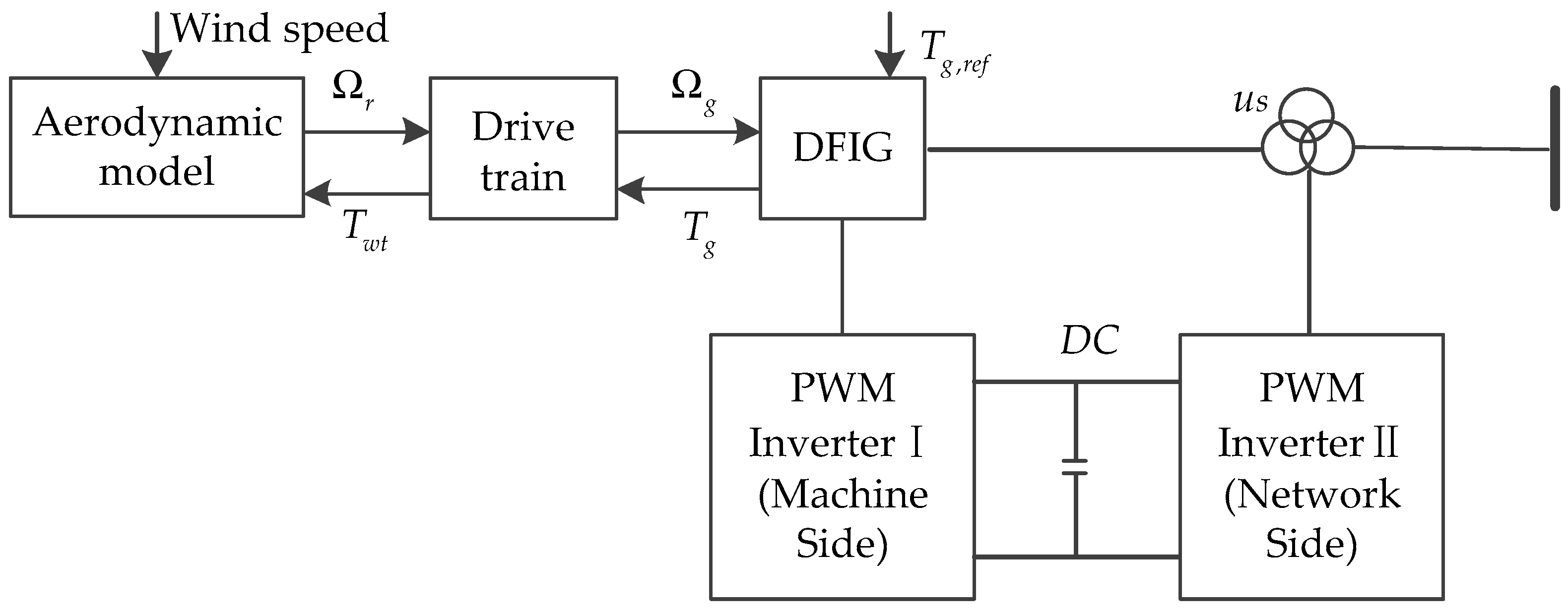
WECS is mainly composed of the wind turbine, transmission system, generator, and power grid. The wind turbine captures wind energy, and converts it into mechanical energy via the wind turbine rotation, which drives the rotor of the doubly fed induction motor to rotate by the transmission system, thus generating electricity, through the converter, to the grid. The overall block diagram of wind energy conversion system with a DFIG is depicted in Figure 1.

Using the kinematics equation of the transmission system [20,21,22], The dynamics model of the wind power generation system Equation (43) can be obtained as follows:

$$\begin{array}{l}\frac{d{\Omega }_r}{dt}=(\frac{D_r}{J_r}+\frac{K_{opt}}{J_r}{\Omega }_r){\Omega }_r-\frac{n_b}{J_r}{T}_h\\ \frac{d{\Omega }_g}{dt}=-\frac{D_g}{J_g}{\Omega }_g+\frac{1}{J_g}{T}_h-\frac{1}{J_g}{T}_g\\ \frac{d{T}_h}{dt}=\frac{1}{n_b}(K_{ls}-\frac{D_r{D}_{ls}}{J_r}+\frac{D_{lse}{K}_{opt}}{J_r}{\Omega }_r){\Omega }_r-\frac{1}{n_{{}_b}^2}(K_{ls}-\frac{D_g{D}_{ls}}{J_g}){\Omega }_g-D_{ls}(\frac{1}{J_r}+\frac{1}{n_b^2{J}_g})T_h+\frac{D_{ls}}{n_{{}_b}^2{J}_g}{T}_g\\ \frac{d{T}_g}{dt}=-\frac{1}{{\tau }_g}{T}_g+\frac{1}{{\tau }_g}{T}_{g,ref}\end{array}$$

(43)

where $K_{opt}=0.5\rho \pi R^5{C}_{p\max }/{\lambda }_{{}_{opt}}^2$, $D_r$ and $D_g$ represent the damping constants of the rotor and the generator respectively, ${\tau }_g$ is the time constant, $K_{ls}$ denotes the equivalent torsional stiffness of the low-speed shaft, $D_{ls}$ is the damping constants of the equivalent low-speed shaft, $T_h$ is the high-speed shaft torque, $J_r$ is the rotor moment of inertia, $J_g$ is the generator moment of inertia, $T_g$ is the generator torque, $T_{g,ref}$ is the required generator torque, ${\Omega }_g$ is the mechanical generator speed and $n_b$ is the gearbox ratio.

From the dynamics model (43), the standard form of WECS equation of state can be expressed as:

$$\begin{array}{l}\dot{x}(t)=A(x)x(t)+Bu(t)\\ y(t)=C(x)x(t)\end{array}$$

(44)

with $x(t)={\left[\begin{array}{cccc}{x}_1& x_2& x_3& x_4\end{array}\right]}^T={\left[\begin{array}{cccc}{\Omega }_r& {\Omega }_g& T_h& T_g\end{array}\right]}^T$, $u(t)=T_{g,ref}$,

$$\begin{gathered} \begin{array}{l}A(x)=\left[\begin{array}{cccc}(\frac{D_r}{J_r}+\frac{K_{opt}}{J_r}{\Omega }_r)& 0& -\frac{n_b}{J_r}& 0\\ 0& -\frac{D_g}{J_g}& \frac{1}{J_g}& -\frac{1}{J_g}\\ a_1+\frac{D_{lse}{K}_{opt}}{n_b{J}_r}{\Omega }_r& a_2& a_3& \frac{D_{ls}}{n_{{}_b}^2{J}_g}\\ 0& 0& 0& -\frac{1}{{\tau }_g}\end{array}\right]\\ \end{array},B=\left[\begin{array}{cccc}0& 0& 0& 0\\ 0& 0& 0& 0\\ 0& 0& 0& 0\\ 0& 0& 0& \frac{1}{{\tau }_g}\end{array}\right],C(x)=\left[\begin{array}{cccc}1& 0& 0& 0\\ 0& 1& 0& 0\\ 0& 0& 0& 0\\ 0& 0& 0& 0\end{array}\right] \\ y(t)=\left[\begin{array}{c}{y}_1\\ y_2\end{array}\right]=\left[\begin{array}{c}{\Omega }_r\\ {\Omega }_g\end{array}\right],a_1=\frac{1}{n_b}(K_{ls}-\frac{D_r{D}_{ls}}{J_r}),a_2=-\frac{1}{n_b^2}(K_{ls}-\frac{D_g{D}_{ls}}{J_g}),a_3=-D_{ls}(\frac{1}{J_r}+\frac{1}{n_b^2{J}_g}) \end{gathered}$$

4.2. T-S Fuzzy Description of WECS

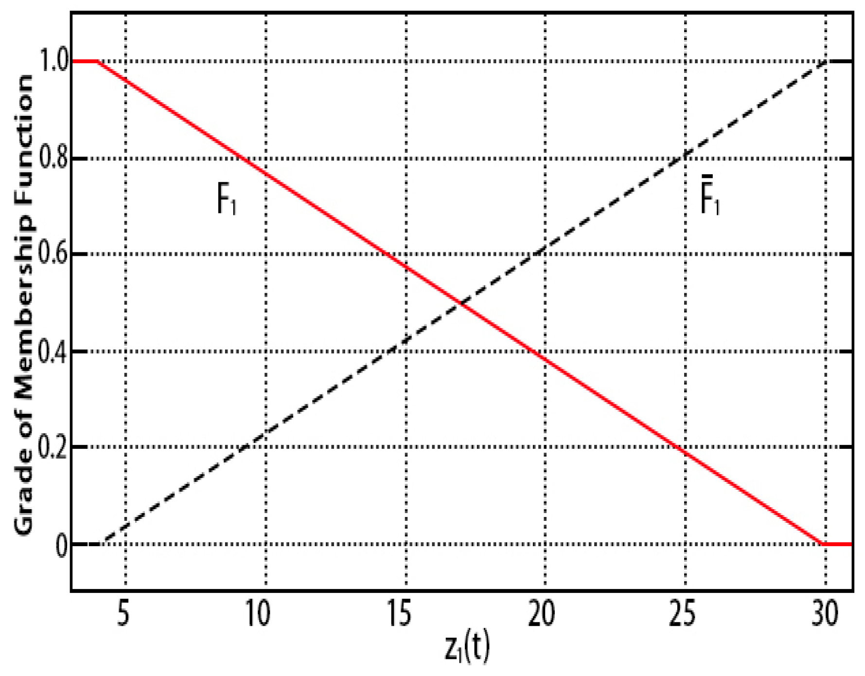
T-S fuzzy is applied to WECS. By looking at the function of the system matrix $A(x)$, the premise variable $z_1(t)={\Omega }_r$ and $z_2(t)={\Omega }_g$ are defined. Then, the membership functions of $z_1(t)$ and $z_2(t)$ are selected $A(x)={\displaystyle \sum _{i=1}^r{u}_i(z(t))}{A}_i$, $B(x)={\displaystyle \sum _{i=1}^r{u}_i(z(t))}{B}_i$, $C(x)={\displaystyle \sum _{i=1}^r{u}_i(z(t))}{C}_i$.

To simplify, the membership function of the two fuzzy subsets can be expressed by Equation (45):

$$\begin{array}{l}{F}_j\left(z_j(t)\right)=\frac{-z_{j\min }}{z_{j\max }-z_{j\min }}(\frac{1}{z_{j\max }-z_{j\min }})z_{jt}\\ {\overline{F}}_j\left(z_j(t)\right)=1-F_j\left(z_j(t)\right)(j=1,2)\end{array}$$

(45)

where the variable $z_{jt}$ is bounded by its upper value $z_{j\min }$ and lower value $z_{j\max }$. The membership functions of $z_1(t)$ are depicted in Figure 2, and each membership function also indicates the model uncertainty of each subsystem. The membership functions of $z_2(t)$ are implemented in the same way.

The T-S fuzzy model with uncertain parameters and actuator failure of WECS (44) can be expressed by the following 4 rules:

Rule 1: If $z_1(t)$ is $F_1^{}$ and $z_2(t)$ is $F_2^{}$

$$\mathrm{Then}\dot{x}(t)=(A_1+\Delta A_1)x(t)+(B_1+\Delta B_1)u(t)+D_{1}d(t)$$

(46)

Rule 2: If $z_1(t)$ is $F_1^{}$ and $z_2(t)$ is ${\overline{F}}_2^{}$

$$\mathrm{Then}\dot{x}(t)=(A_2+\Delta A_2)x(t)+(B_2+\Delta B_2)u(t)+D_{2}d(t)$$

(47)

Rule 3: If $z_1(t)$ is ${\overline{F}}_1^{}$ and $z_2(t)$ is $F_2^{}$

$$\mathrm{Then}\dot{x}(t)=(A_3+\Delta A_3)x(t)+(B_3+\Delta B_3)u(t)+D_{3}d(t)$$

(48)

Rule 4: If $z_1(t)$ is ${\overline{F}}_1^{}$ and $z_2(t)$ is ${\overline{F}}_2^{}$

$$\mathrm{Then}\dot{x}(t)=(A_4+\Delta A_4)x(t)+(B_4+\Delta B_4)u(t)+D_{4}d(t)$$

(49)

Therefore, the global fuzzy model of wind energy conversion system is presented by:

$$\begin{array}{l}\dot{x}(t)={\displaystyle \sum _{i=1}^4{u}_i(z(t))}\left[(A_i+\Delta A_i)x(t)+(B_i+\Delta B_{{}_i})u(t)+D_{i}d(t)\right]\\ y(t)={\displaystyle \sum _{i=1}^4{u}_i(z(t))}{C}_{i}x(t)\hspace{1em}\hspace{1em}i=1,2,3,4\end{array}$$

(50)

where

$$\begin{gathered} A_i+\Delta A_i=\left[\begin{array}{cccc}(\frac{D_r}{J_r}+\frac{K_{opt}}{J_r}{z}_{1i})& 0& -\frac{n_b}{J_r}& 0\\ 0& -\frac{D_g}{J_g}& \frac{1}{J_g}& -\frac{1}{J_g}\\ a_1+\frac{D_{lse}{K}_{opt}}{n_b{J}_r}{z}_{1i}& a_2& a_3& \frac{D_{ls}}{n_{{}_b}^2{J}_g}\\ 0& 0& 0& -\frac{1}{{\tau }_g}\end{array}\right],B_i+\Delta B_{{}_i}=\left[\begin{array}{cccc}0& 0& 0& 0\\ 0& 0& 0& 0\\ 0& 0& 0& 0\\ 0& 0& 0& \frac{1}{{\tau }_g}\end{array}\right] \\ {C}_i=\left[\begin{array}{cccc}1& 0& 0& 0\\ 0& 1& 0& 0\\ 0& 0& 0& 0\\ 0& 0& 0& 0\end{array}\right],D_i=\left[\begin{array}{c}1\\ 1\\ 0\\ 0\end{array}\right] \end{gathered}$$

$\Delta A_i$ and $\Delta B_{{}_i}$ represent the system parameter bounded uncertainties, with $\Delta B_{{}_i}=0$. The change of the parameter uncertainties $\Delta J_g$ within 30% and 50% of nominal value is considered. From Equation (6), we can get $c=6$, $s=64$. Therefore, the fuzzy uncertainty is given by $\Delta A_i={\displaystyle \sum _{l=1}^{64}{h}_l}\Delta {\tilde{A}}_l$. Then, Equation (28) of WECS fuzzy model can be presented as:

$$\dot{x}(t)={\displaystyle \sum _{i=1}^4{\displaystyle \sum _{l=1}^{64}{u}_i{h}_l}}\left[(A_i+\Delta {\tilde{A}}_l)x(t)+B_{i}u(t)+D_{i}d(t)\right]$$

(51)

From (18), The inferred output of the FRSFTC is:

$$u(t)={\displaystyle \sum _{j=1}^4{\displaystyle \sum _{l=1}^{64}{u}_j{h}_l}}\left[-L_{jl}{\widehat{x}}_o(t)-{\overline{D}}_j\widehat{d}(t)+r(t)\right]$$

(52)

5. Simulation Analysis

Based on system model (50), a WECS with low power (6KW) and high speed is simulated in MATLAB/Simulink environment (R2014a, MathWorks, Natick, MA, USA). The parameters of the simulation system are depicted in

Table 1. Simulation Parameters.

Parameter Names	Values
Rated power $P_n$	$6\mathrm{KW}$
Rated voltage $V_s$	$220\mathrm{V}$
Rated speed $w_s$	$100\mathsf{\pi }\mathrm{rad}/\mathrm{s}$
Air density $\rho$	$1.25{\mathrm{kg}/\mathrm{m}}^3$
Blade length $R$	$2.5\mathrm{m}$
Transmission efficiency $\eta$	$0.95$
Pole pairs $p$	$2$
Rated electromagnetic torque $T_g$	$40\mathrm{N}\cdot \mathrm{m}$
Inertia of the generator $J_g$	$0.0092\mathrm{kg}\cdot {\mathrm{m}}^2$
Inertia of the rotor $J_r$	$3.6\mathrm{kg}\cdot {\mathrm{m}}^2$

:

As the actuator of the entire WECS, the transmission system is mainly caused by faults such as deviation, drift and so on [23,24]. To facilitate the research and simulation, this paper only considers the actuator faults and does not involve unknown external interference. Accordingly, the drift, deviation and mixed fault of the actuator are considered in the simulation design, and as shown below:

$$d(t)=\{\begin{array}{ll}4\sin \pi t& \hspace{1em}50\mathrm{s}\le t<60\mathrm{s}\\ 3& \hspace{1em}60\mathrm{s}\le t<70\mathrm{s}\\ 2.5+2\sin 0.5\pi t& \hspace{1em}70\mathrm{s}\le t<80\mathrm{s}\end{array}$$

(53)

Case 1: The change of the parameter uncertainties $\Delta J_g$ within 30% of nominal value is considered.

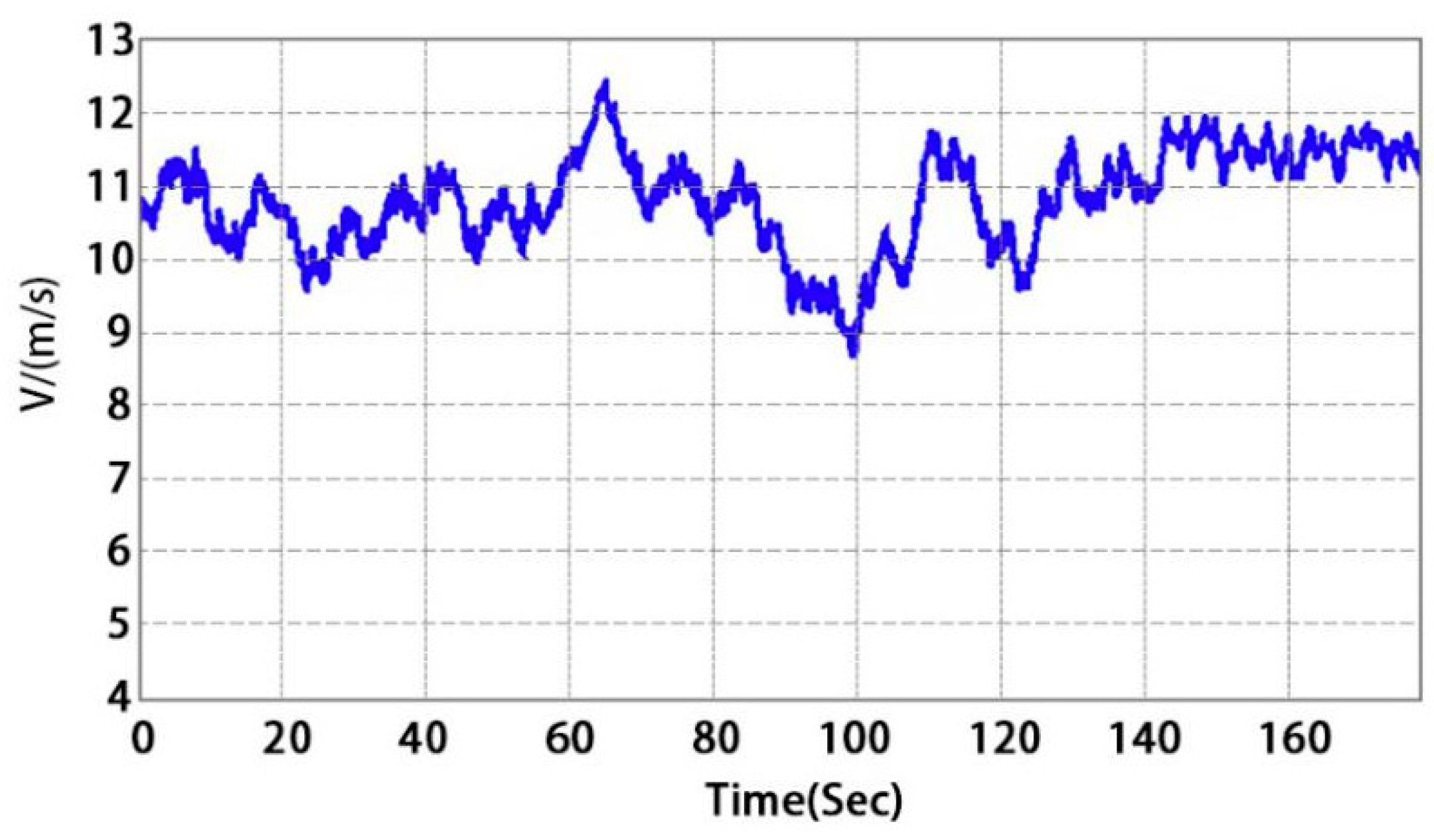
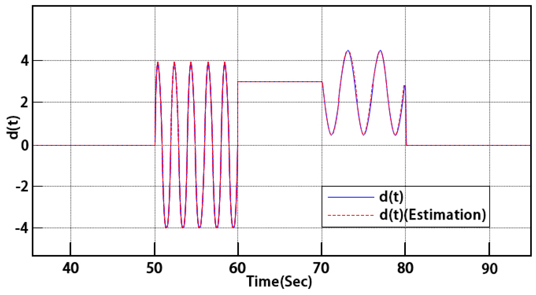
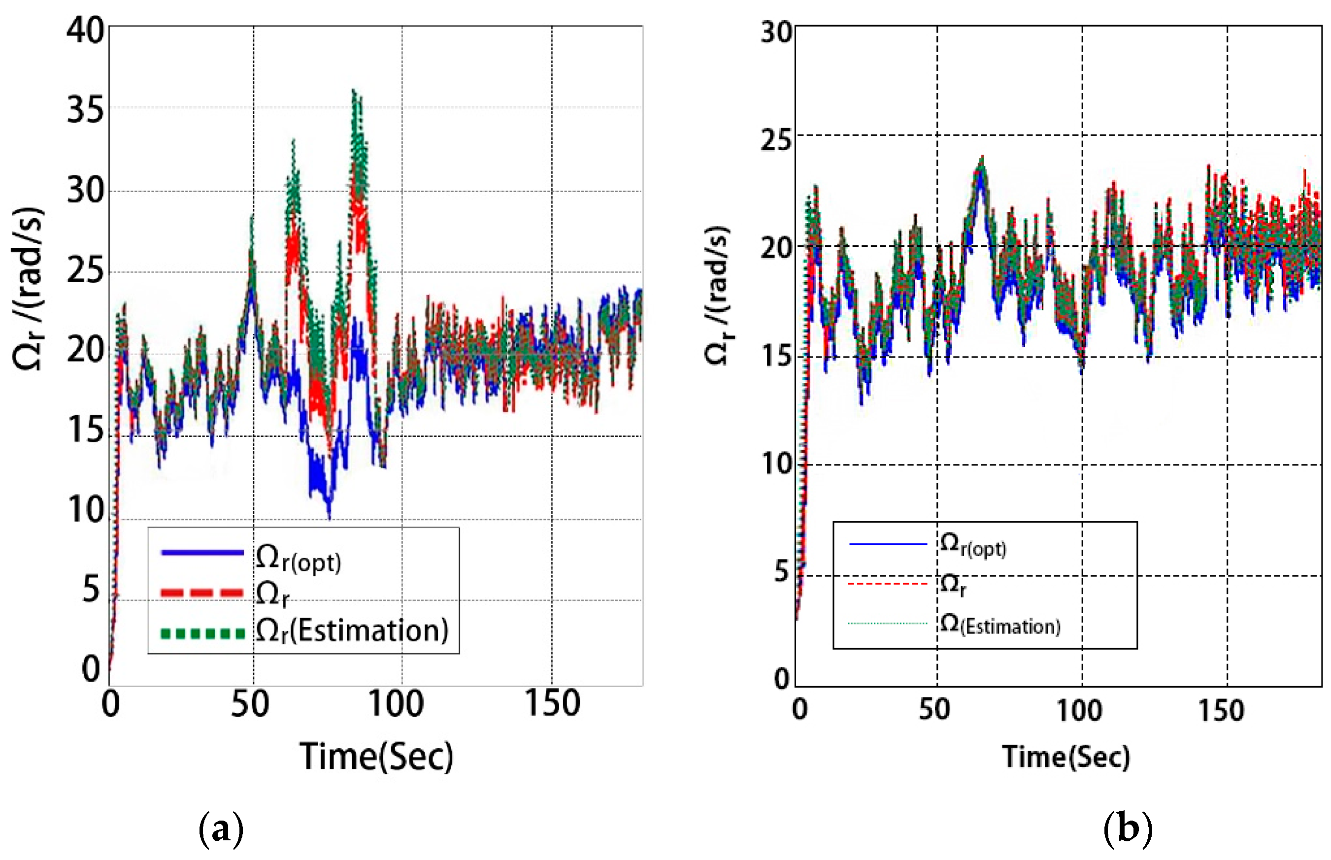
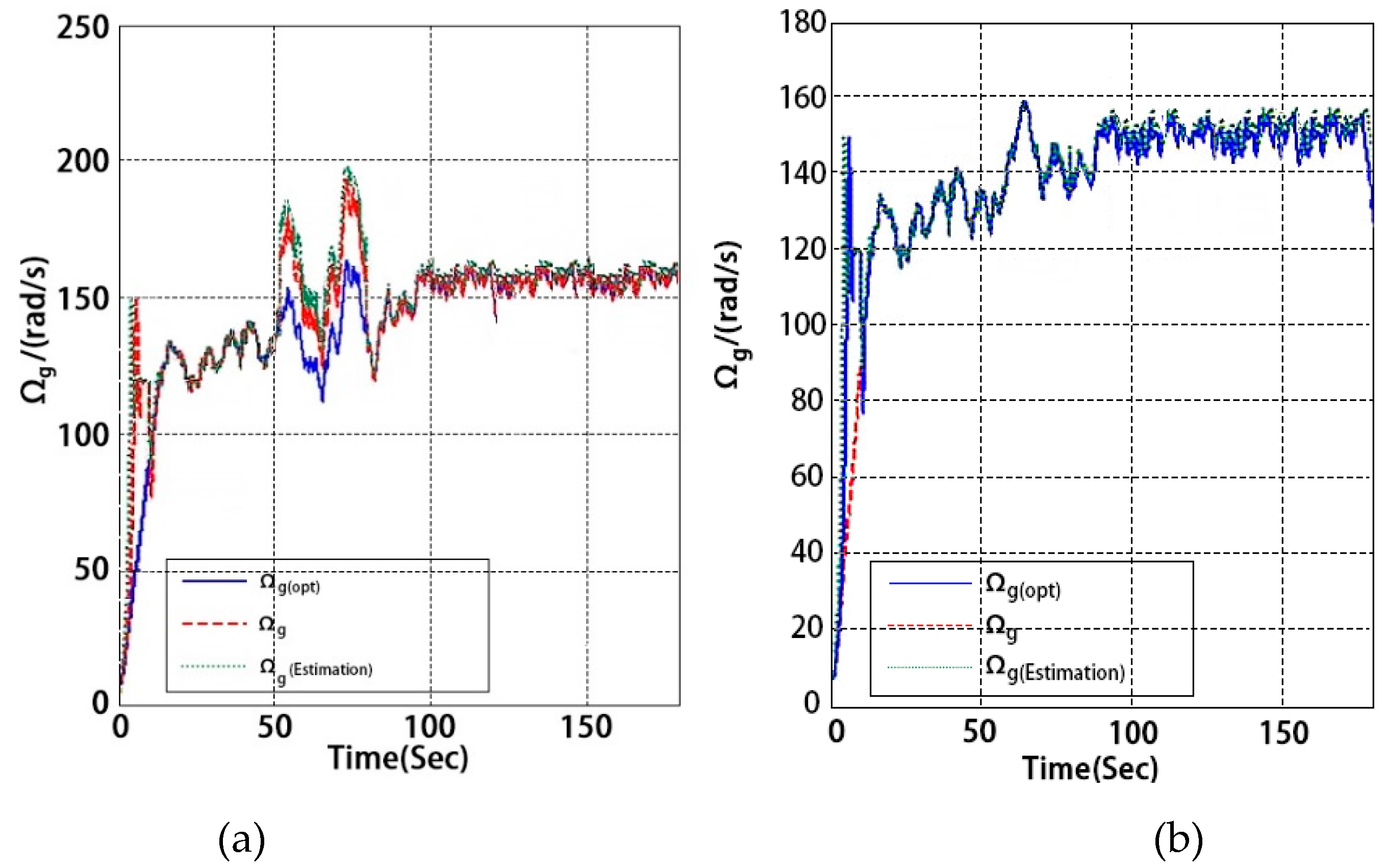
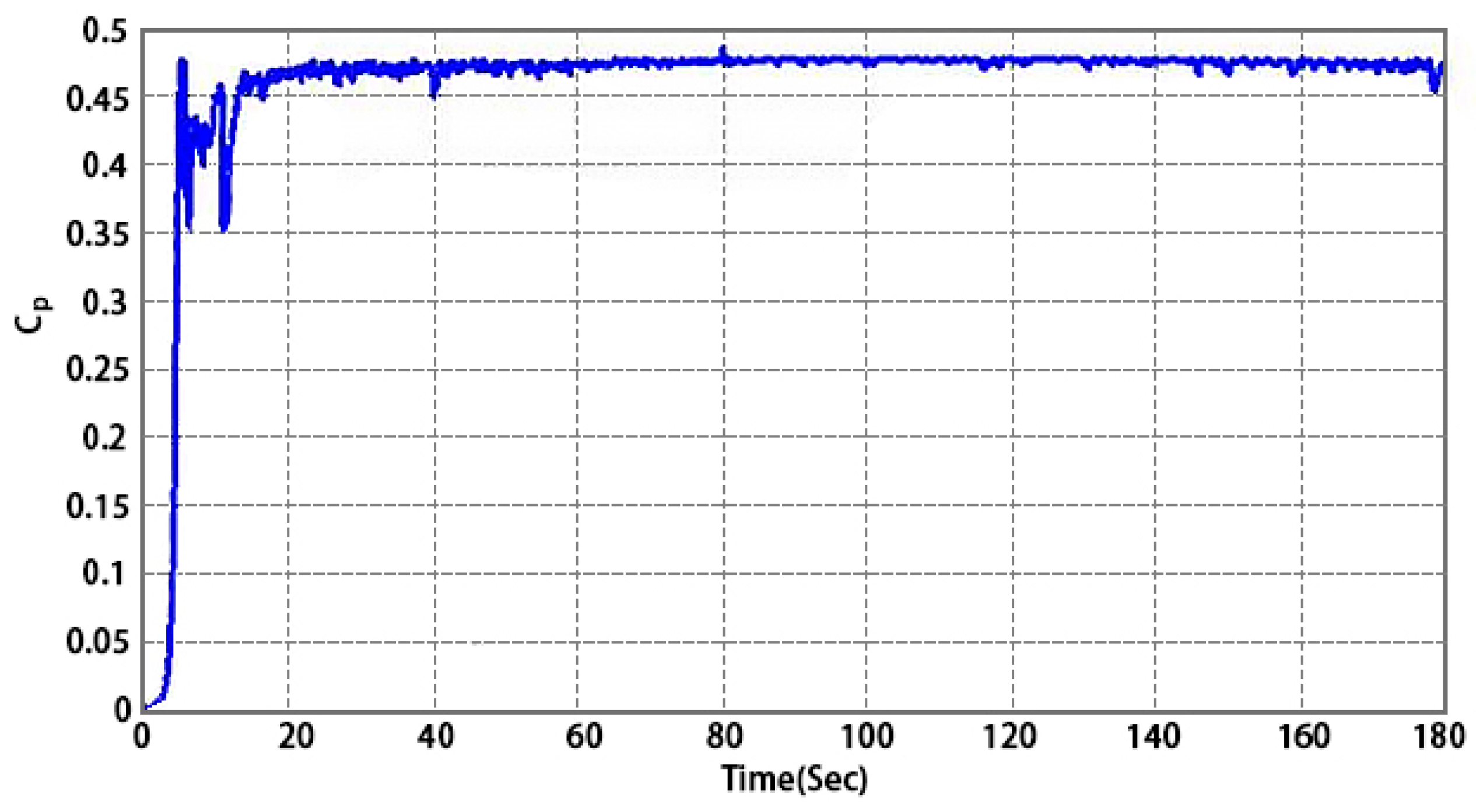
The controller is tested according to the random change of wind speed. Figure 3 is the wind speed waveform, Figure 4 is the actual and estimated value of time-varying fault signal, it can be seen that the designed observer can rapidly and accurately reconstruct the fault information of the system. When the system fails, the operation of the system with and without FRSFTC strategy is shown in Figure 5, Figure 6, Figure 7 and Figure 8, Figure 9 shows the power coefficient when FRSFTC is adopted in the case of actuator faults.

Comparing (a) and (b) in Figure 5 and Figure 6, it can be seen that between $t=50\mathrm{s}$ and $t=80\mathrm{s}$, when the actuator of the system fails, both the trajectories of ${\Omega }_r$ and ${\Omega }_g$ have abrupt changes, and the oscillation amplitude increases and cannot be maintained in the optimal position. However, under the FRSFTC strategy, the system of low- and high-speed fluctuation range is reduced. The system failure of gear and bearing fault impact and oscillation are greatly reduced.

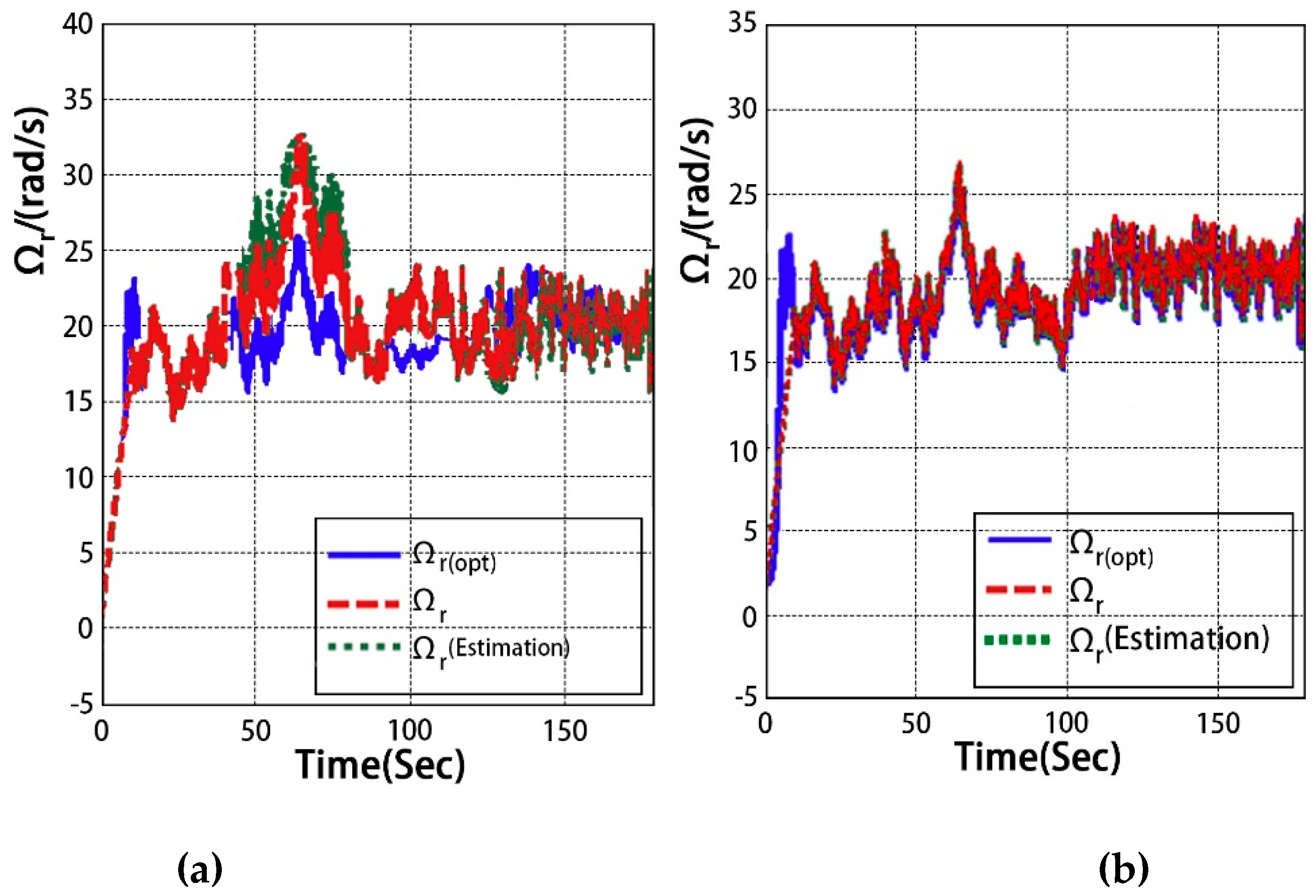
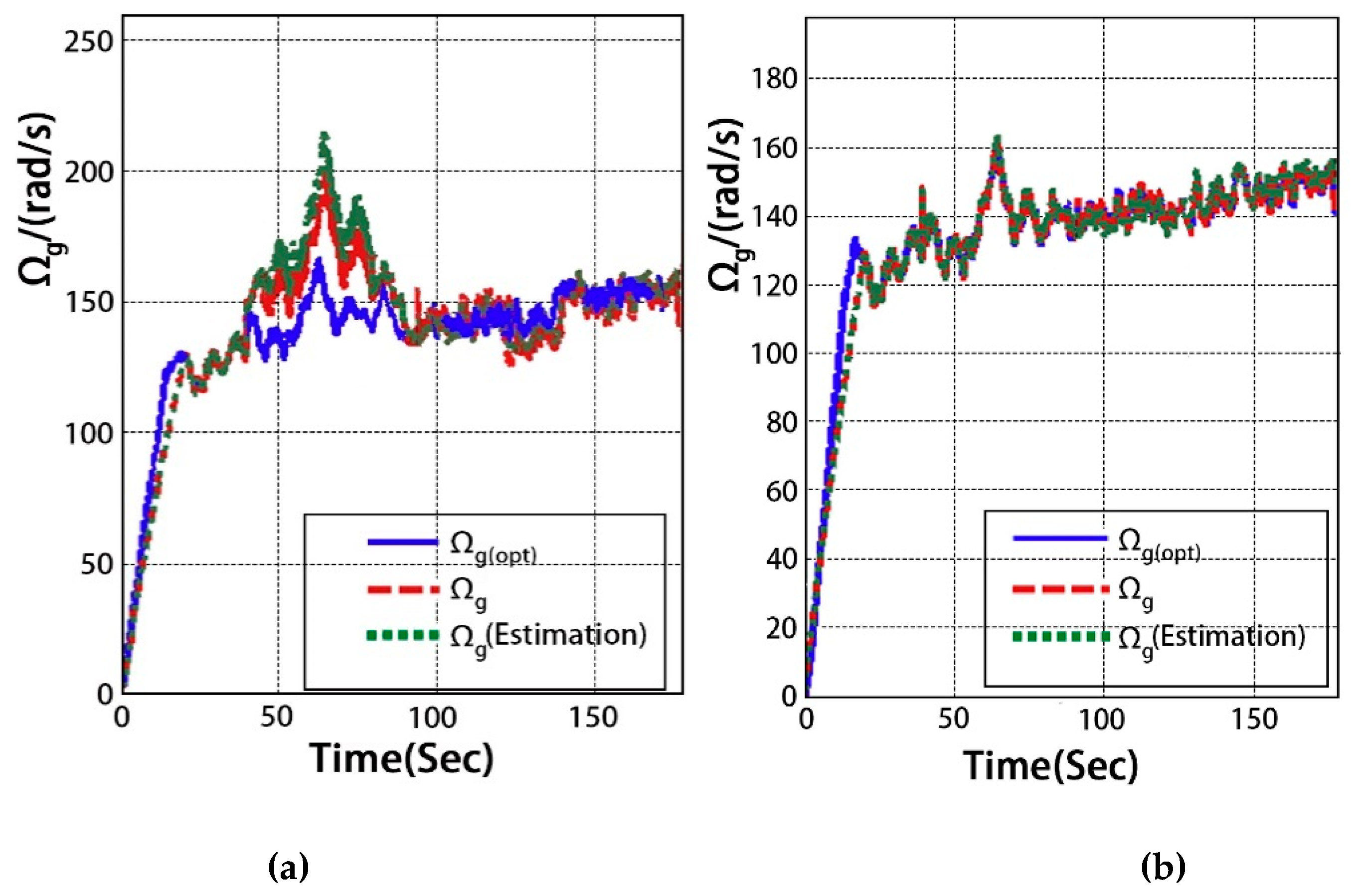
Case 2: The change of the parameter uncertainties $\Delta J_g$ within 50% of nominal value is considered.

According to simulation results depicted in Figure 7 and Figure 8, it can be seen from the comparison between (a) and (b) when the parameter uncertainty $\Delta J_g$ is within 50% of nominal value, the designed FRSFTC strategy can still reduce the fluctuation range of the system at low speed and high speed and achieve a good fault-tolerance control effect.

The power coefficient is shown in Figure 9, and the $C_{p\max }\approx 0.48$, which shows that when the actuator fails, the WECS can achieve maximum wind energy capture.

In summary, the simulation results show that when the actuator fault occurs, considering the uncertainty of the system, the proposed FRSFTC strategy can achieve the maximum wind energy capture at the rated wind speed and improve the use rate of the wind turbine when the actuator fault occurs.

6. Conclusions

This paper presents the idea of robust fault-tolerant control based on system state estimation and fault reconstruction for parameter-uncertain nonlinear systems with actuator faults. We first introduce the T-S fuzzy model of the nonlinear system, and then a fuzzy scheduling fault-tolerant controller based on observer fault reconstruction is proposed for the uncertainty, unmeasurable state, and actuator fault of the system. The gain of controller and observer is obtained by solving LMIS. Finally, according to the Taylor series and Lyapunov stability theory, the sufficient and necessary conditions for the stability of the closed-loop system in the event of actuator failure are given, and fault-tolerance integrity of the system is realized. Finally, the WECS is taken as an example for analysis. Simulation results show that considering the uncertainty of the system, when the actuator fails, the FRSFTC can improve the efficiency of wind energy capture at a rated wind speed while ensuring the normal operation of all states of the system. The feasibility and effectiveness of the proposed fault-tolerant control strategy are verified.

References

- Tiwari, R.; Babu, N.R. Recent developments of control strategies for wind energy conversion system. Renew. Sustain. Energy Rev. 2016, 66, 268–285. [Google Scholar] [CrossRef]
- Dai, J.C.; Xin, Y.; Li, W. Development of wind power industry in China: A comprehensive assessment. Renew. Sustain. Energy Rev. 2018, 97, 156–164. [Google Scholar] [CrossRef]
- Cruz, M.R.M.; Fitiwi, D.Z.; Santos, S.F.; Mariano, S.J.P.S.; Catalão, J.P.S. Prospects of a meshed electrical distribution system featuring large-scale variable renewable power. Energies 2018, 11, 3399. [Google Scholar] [CrossRef]
- Nguyen, C.-K.; Nguyen, T.-T.; Yoo, H.-J.; Kim, H.-M. Consensus-based SOC balancing of battery energy storage systems in wind farm. Energies 2018, 11, 3507. [Google Scholar] [CrossRef]
- Pozo, F.; Vidal, Y. Wind turbine fault detection through principal component analysis and statistical hypothesis testing. Energies 2016, 9, 3. [Google Scholar] [CrossRef]
- Pérez, J.M.P.; Márquez, F.P.G.; Tobias, A. Wind turbine reliability analysis. Renew. Sustain. Energy Rev. 2013, 23, 463–472. [Google Scholar] [CrossRef]
- Shi, Y.; Hou, Y.; Sun, D.; Li, Z. Stochastic modelling and H∞fault tolerance control of WECS. Electr. Mach. Control 2015, 19, 100–110. [Google Scholar]
- Cho, S.; Gao, Z.; Moan, T. Model-based fault detection, fault isolation and fault-tolerant control of a blade pitch system in floating wind turbines. Renew. Energy 2018, 120, 306–321. [Google Scholar] [CrossRef]
- Wu, Z.; Yang, Y.; Xu, C. Fault diagnosis and initiative tolerant control for wind energy. Chin. J. Mech. Eng. 2015, 9, 112–118. [Google Scholar] [CrossRef]
- Xiao, J.; Zhao, T. Overview and prospect of T-S fuzzy control. J. Southwest Jiaotong Univ. 2016, 51, 462–474. [Google Scholar]
- Kwon, O.M.; Park, M.J.; Ju, H.P. Stability and stabilization of T-S fuzzy systems with time-varying delays via augmented Lyapunov-Krasovskii functionals. Inf. Sci. 2016, 372, 1–15. [Google Scholar] [CrossRef]
- Zhu, F.; Jiang, P.; Li, X. Design of observer and dynamic output feedback fault tolerant controller based on T-S fuzzy model. J. Xi’an Jiaotong Univ. 2016, 50, 91–96. [Google Scholar]
- Zhai, D.; Lu, A.; Dong, J. Event triggered H−/H ∞ fault detection and isolation for T-S fuzzy systems with local nonlinear models. Signal Process. 2017, 138, 244–255. [Google Scholar] [CrossRef]
- Li, H.; Gao, Y.; Wu, L. Fault detection for T-S fuzzy time-delay systems: Delta operator and input-output methods. IEEE Trans. Cybern. 2015, 45, 229–241. [Google Scholar] [CrossRef] [PubMed]
- Li, X.; Luo, X.; Li, S.; Guan, X. Output consensus for heterogeneous nonlinear multi-agent systems based on T-S fuzzy model. J. Syst. Sci. Complex. 2017, 30, 1042–1060. [Google Scholar] [CrossRef]
- Hao, S.; Lei, S.; Ju, H. Reliable mixed H ∞/passive control for T–S fuzzy delayed systems based on a semi-Markov jump model approach. Fuzzy Sets Syst. 2017, 314, 79–98. [Google Scholar]
- Shaker, M.S.; Patton, R.J. Active sensor fault tolerant output feedback tracking control for wind turbine systems via T–S model. Eng. Appl. Artif. Intell. 2014, 34, 1–12. [Google Scholar] [CrossRef]
- Abdelmalek, S.; Barazane, L.; Larabi, A. A novel scheme for current sensor faults diagnosis in the stator of a DFIG described by a T-S fuzzy model. Measurement 2016, 91, 680–691. [Google Scholar] [CrossRef]
- Li, S.; Wang, H.; Aitouche, A. Active fault tolerant control of wind turbine systems based on DFIG with actuator fault and disturbance using Takagi–Sugeno fuzzy model. J. Frankl. Inst. Eng. Appl. Math. 2018, 355, 8194–8212. [Google Scholar] [CrossRef]
- Gálvez-Carrillo, M.; Kinnaert, M. Sensor fault detection and isolation in doubly fed induction generators accounting for parameter variations. Renew. Energy 2011, 36, 1447–1457. [Google Scholar] [CrossRef]
- Chitti, B.B.; Mohanty, K.B. Doubly-fed induction generator for variable speed wind energy conversion systems e modeling & simulation. Int. J. Comput. Electr. Eng. 2010, 2, 141–147. [Google Scholar]
- Di Giorgio, A.; Pimpinella, L.; Mercurio, A. A feedback linearization based wind turbine control system for ancillary services and standard steady state operation. In Proceedings of the 18th Mediterranean Conference on Control & Automation, Marrakech, Morocco, 23–25 June 2010; pp. 1585–1590. [Google Scholar]
- Shen, Y.; He, Q.; Yang, X.; Zhao, Z. Actuator fault reconstruction and fault-tolerant control of wind energy conversion system. Control Theor. Appl. 2015, 32, 413–420. [Google Scholar]
- Zhou, D.; Ye, Y. Modern Fault Diagnosis and Fault-Tolerant Control, 1st ed.; Tsinghua University Press: Beijing, China, 2000; pp. 299–306. [Google Scholar]
Figure 1.
Overall block diagram of the wind energy conversion system (WECS) with a doubly fed induction generators (DFIG).
Figure 2.
The membership functions of .
Figure 3.
Wind speed.
Figure 4.
Actuator faults signal and its estimate.
Figure 5.
The trajectories of . (a) Without using the FRSFTC strategy; (b) Using the FRSFTC strategy.
Figure 6.
Figure 7.
Figure 8.
Figure 9.
Power coefficient.