Feasibility Study of Freeze Recovery Options in Parabolic Trough Collector Plants Working with Molten Salt as Heat Transfer Fluid

Abstract

Parabolic trough collector (PTC) technology is currently the most mature solar technology, which has led to the accumulation of relevant operational experience. The overall performance and efficiency of these plants depends on several components, and the heat transfer fluid (HTF) is one of the most important ones. Using molten salts as HTFs has the advantage of being able to work at higher temperatures, but it also has the disadvantage of the potential freezing of the HTF in pipes and components. This paper models and evaluates two methods of freeze recovery, which is needed for this HTF system design: Heat tracing in pipes and components, and impedance melting in the solar field. The model is used to compare the parasitic consumption in three molten salts mixtures, namely Solar Salt, HiTec, and HiTec XL, and the feasibility of this system in a freezing event. After the investigation of each of these subsystems, it was concluded that freeze recovery for a molten salt plant is possible.

1. Introduction

Today, current trends in energy supply are unsustainable from environmental, economic, and social points of view, and stricter low-carbon economy policies push this demand further. Therefore, the development of advanced energy technologies is very much needed [1,2]. Crucial players to achieve such sustainable development goals are renewable energies, and in this new scenario concentrated solar power (CSP) is one of the most interesting alternatives [3,4].

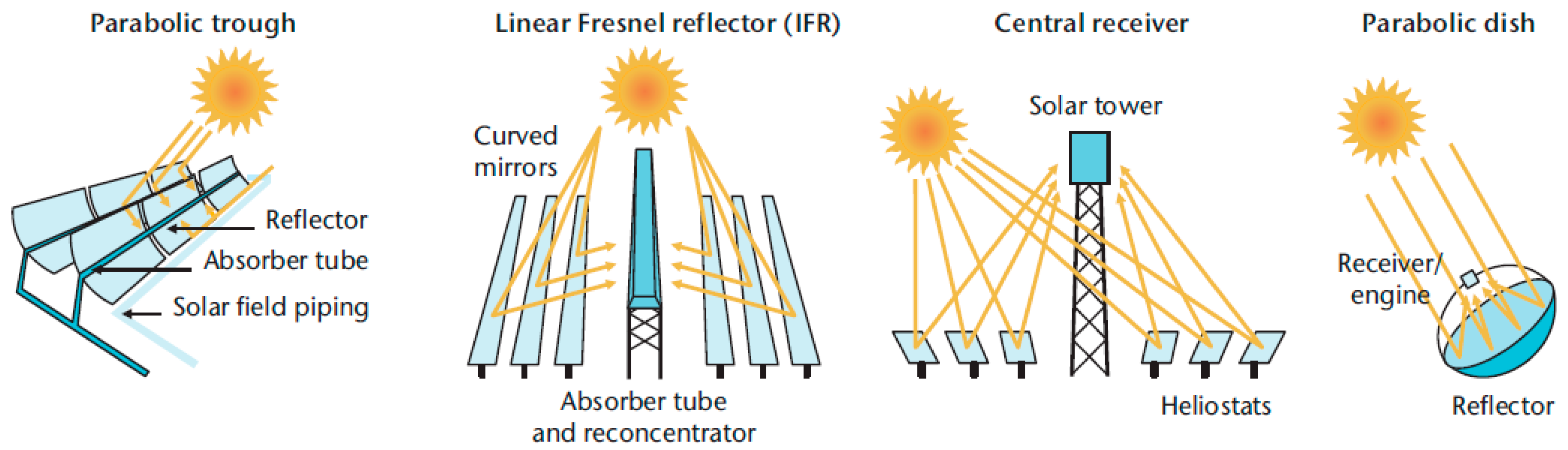
Parabolic trough, linear Fresnel, tower, and parabolic dish are the main different options in CSP technology, depending on how the focus of sunrays and the position of the receiver is implemented (Figure 1). Line focus systems track the sun with mirrors arranged in one axis (parabolic trough and linear Fresnel systems), while point focus systems use two axes (tower and dish systems). On the other hand, the receiver can be fixed (linear Fresnel and tower systems) or mobile (parabolic trough and dish systems).

Parabolic trough collector (PTC) systems concentrate the sun in a parabolically curved trough-shaped reflector. The receiver is a tube located along the inner side of the collector [5]. The heat transfer fluid (HTF), usually synthetic oil, is heated by the energy concentrated in the receiver, where it flows through the tube along the trough collector and is then used to generate electricity in a conventional steam turbine generator after a heat transfer exchange with a secondary HTF, water/steam.

The tower technology uses large sun-tracking mirrors, also called heliostats, to focus the sunlight on a receiver that is located at the top of the tower to produce electricity from the sun [5]. The HTF is usually molten salt or water/steam, and it is heated when it flows through the receiver. Again, it is used in a conventional steam turbine generator to produce electricity, either directly or by using a heat exchanger.

The linear Fresnel technology [6], on the other hand, uses mirrors mounted on trackers on the ground that are flat or slightly curved. The mirrors reflect sunlight to a receiver tube located above them. Sometimes, a small parabolic mirror is placed on the receiver to increase the focus of the sunlight.

The last technology is parabolic dish systems, in which the concentrator is a dish with a parabolic-shaped focus point, with the receiver located at the focal point [5]. The sun is tracked with a two-axis structure where the concentrators are mounted. The receiver is usually mounted next to the heat engine that uses the collected heat to produce electricity on site. Here, Stirling and Brayton cycle engines are used.

The HTF, thermal energy storage (TES), and power cycle can be selected from different options in each technology. One of the most important components to achieve high overall performance and efficiency in CSP systems is the HTF [7]. The main requirements for a proper HTF were summarized by Benoit et al. [8], based on the review of existing and potential HFTs used in CSP receivers. To increase the efficiency of the cycle, the HTF should be able to work in a wide working temperature range and should present high thermal stability. If this is accomplished, the cost of the solar field, which is the main saving factor in a CSP plant, is reduced. Next, in order to increase the heat transfer between the HTF, the TES material, and the power block driving fluid, and in addition to withstand high pressure and temperature changes, the HTF should have good thermophysical properties. Finally, the HTF should be non-hazardous, have a low corrosive behaviour, and should be cost-effective. More information about different types of HTF suitable for CSP plants and other high temperature applications (such as liquids, supercritical fluids, and gases) is presented in other studies [7,9,10], such information on their cost and thermal and physical properties.

CSP technology with a PTC system is currently the most mature solar technology, leading to the accumulation of relevant operational experience [11]. The most widely used heat transfer fluid (HTF) in parabolic trough plants is a eutectic mixture of the organic compounds biphenyl oxide and diphenyl oxide [12,13,14]. The operation temperature of the solar thermal power plant is limited to up to 400 °C when using an organic HTF [14,15], since when operating above this temperature the HTF degrades [15].

Significantly higher efficiency of the solar thermal power system can be achieved if a more stable HTF is used, such as binary or ternary mixtures of nitrate salts within the needed operating temperature [15,16,17]. These eutectic mixtures would allow operating temperatures of 500 °C or higher [10,16]. The most widely considered candidates are Solar Salt, HiTec^®, and HiTec XL^® [12,18]. Solar Salt is a binary salt mixture of 60 wt.% NaNO₃ and 40 wt.% KNO₃. HiTec is a ternary mixture of alkali-nitrates/nitrites, and finally, HiTec XL is a ternary mixture of sodium, potassium, and calcium nitrates. Their melting properties are given in

Table 1. Properties of the three heat transfer fluid (HTF) candidates [12,19,20].

Solar Salt
Composition (by weight)	60% NaNO3, 40% KNO3
Freeze Temperature, °C	220–238 (non-eutectic range at this mixture)
Density, kg/m3	2090 − 0.636 × T (°C)
Specific heat, J/kg C	1443 + 0.172 × T (°C)
Dynamic Viscosity, Pa·s	(22.14 − 0.120 × T (°C) + 2.281 × 10 −4 × (T (°C))2 − 1.474 × 10−7 × (T (°C))3)/1000
Thermal conductivity, W/m °C	0.443 + 1.9 · 10−4 × T (°C)
Hitec®
Composition (by weight)	40% NaNO2, 7% NaNO3, 53% KNO3
Freeze Temperature, °C	142 (eutectic point)
Density, kg/m3	2080 − 0.733 × T (°C)
Specific heat, J/kg C	1.56
Dynamic Viscosity, Pa·s	0.00622 − 0.0000102 × T(°C)
Thermal conductivity, W/m °C	0.588 − 0.000647 × T (°C)
Hitec XL®
Composition (by weight)	7% NaNO2, 45% KNO3, 48% Ca(NO3)2
Freeze Temperature, °C	120 (eutectic point)
Density, kg/m3	2240 − 0.8266 × T (°C)
Specific heat, J/kg C	1536 − 0.2624 × T (°C) − 0.0001139 × (T (°C))2
Dynamic Viscosity, Pa·s	1,372,000 × (T (°C)) −3.364
Thermal conductivity, W/m °C	0.519

.

The biggest drawback of these nitrate salt mixtures is that they freeze inside the tubing in the system, since their melting points vary from 120 °C to 220 °C. Therefore, freeze protection has to be considered in any PTC plant. On the other hand, HiTec XL and HiTec have a lower melting point, therefore the problem of freezing is easier to control. On the other hand, the thermal stability of these mixtures is lower than Solar Salt [10,12,19,20].

The benefit of using molten salts as heat transfer fluids results from the increase in the allowable maximum operating temperature [15,21]. However, molten salts with the desired thermal stability limit have freezing/melting points well above ambient temperature. As such, a freeze protection and recovery system (freeze P/R) is needed for three key functions:

• Pre-heat plant for initial salt fill, or pre-heat loops for fill after maintenance.
• Prevent freeze events for the duration of the plant life.
• Recovery from freeze events for the duration of the plant life.

Preheating of the plant is required to prevent the formation of salt plugs during the initial plant fill and to minimize thermal shock to piping and equipment. Preheating will be needed on a loop level to refill the loop with salt after maintenance has been performed on a loop. Once the plant is filled with salt, the system will then be used to prevent freeze events by maintaining a temperature above the freeze point of the salt, should such situations arise. If a plug or blockage does form anywhere in the plant, the system will apply heat to the affected zone to prevent a larger freezing event and/or melt the frozen zone. The freeze P/R system is not intended to provide heating under normal operation of the plant.

The freeze protection/recovery system proposed in this paper includes two main sections: Heat tracing and impedance heating [22,23]. Heat tracing involves the application of heat trace cables to all plant surfaces that might be compromised in a freeze event. This includes all pipes, headers, joints, and valves [24]. If the plant undergoes a freeze risk, the salt in these areas must be melted. Since no external energy hits these components during normal operation, heat tracing is the only practical option of introducing a heat input.

Impedance melting is accomplished by applying a voltage over a necessary number of absorber tubes in the solar field. This voltage, given a resistivity of the tube, induces a current in the absorber tube that results in a heat generation term.

A good understanding of the working philosophy of freeze protection systems is needed to minimize the parasitic consumption of solar plants, being one of the criteria to select the final HTF in the parabolic trough collector plants. Different modelling studies have been published for state-of-the-art of PTC plants [11,25]. However, state-of-the-art PTC plants have never been the subject of a specific feasibility study of heat tracing systems when using high melting point salts as a HTF. The work carried out in this document describes the freeze protection systems used in parabolic trough plants with three mixtures of molten salt, and the modelling for their implementation and optimization in the plant performance model.

2. Heat Tracing

2.1. Heat Trace System Description

The scope of the heat trace study was to develop the capability of predicting heat tracing requirements for salt HTF plants. Heat tracing is accomplished by the application of resistive heating cables being applied to the surface to be heated. These cables produce large heat generation terms when a direct electrical current is applied to them. This heat generation term can be used for freeze recovery or system preheating. Figure 2 shows several ways heat trace cables are mounted to different piping elements, such as pipes, valves, and joints.

The only type of heat trace cable that can withstand the required exposure temperatures over 250 °C are those using mineral insulated (MI) cable. Mineral wool thermal insulation with an aluminium jacket will be used on all traced piping. Mineral wool insulation will be used on valve bodies and bonnets with removable blankets on the actuators. The system has one redundant cable per heat trace zone and this redundant cable will be on header and feeder piping, but not loop and drop-down piping. The systems were designed with the premise that feeder pipes and headers must never freeze.

2.2. Model Description

The schematic shown below in Figure 3 shows a cross section of the pipe, the heat transfer mechanisms that result in heat losses from the heat transfer fluid, and the location of heat addition from the heating system.

The heat tracing system will be placed directly onto the surface of the steel pipe. While the heating cables are in discrete locations, they will be approximated as being evenly distributed over the entire surface of the pipe. Insulation will then be placed around the pipe and heat tracing system. The insulation will, if necessary, consist of high temperature insulation at the inner surface, followed by lower temperature insulation. If the cost of insulation is high, a multilayer configuration can be used, using a first layer of greater performance and cost that is in contact with the cable, and a second layer of lower cost on the external side. The two layers of insulation will ensure that the insulation functions properly at high temperatures but also cuts down on the overall cost of the insulation. Finally, an aluminium cladding will effectively seal the pipe and provide insulation from precipitation and protect it from unforeseen abuse during operation. The heat transfer fluid will flow through the pipe, resulting in heat loss through the pipe walls and out to the ambient surroundings.

The total length of heat trace cable necessary for headers, valves, joints, and pipes is calculated based on the preheat and melting conditions and pipe diameters.

The heat from the HTF will be lost through convective heat transfer with the inner pipe surface. This heat will then be transferred by conduction through the pipe wall, insulations, and the aluminium cladding. Finally, the heat is lost to the ambient surroundings by radiation and convective heat transfer. In addition, the potential for internal heat addition is supplied by the heat tracing system. This heater will be able to supply heat to the pipe walls. The schematic in Figure 4 shows the thermal circuit. In practice, heat loss also occurs at the pipe supports, but this will be ignored for this optimization. It is also worth noting that the radiation losses are to the sky, while the external convection losses are to the surroundings. For this subroutine, it has been assumed that both the radiation and convection losses occur to the ambient surroundings, as indicated in Figure 3. The dashed line indicates that the outer insulation is an option that may be necessary.

The equations for the thermal resistances are:

$$\begin{array}{llll}{R}_{conv,1}^{\prime }=\frac{1}{2\pi h_1{r}_1}& R_{pipe}^{\prime }=\frac{\ln \left(\frac{r_2}{r_1}\right)}{2\pi k_{pipe}}& R_{ins,1}^{\prime }=\frac{\ln \left(\frac{r_3}{r_2}\right)}{2\pi k_{ins,1}}& R_{ins,2}^{\prime }=\frac{\ln \left(\frac{r_4}{r_3}\right)}{2\pi k_{ins,2}}\\ R_{Al}^{\prime }=\frac{\ln \left(\frac{r_5}{r_4}\right)}{2\pi k_{Al}}& R_{conv,2}^{\prime }=\frac{1}{2\pi h_2{r}_5}& R_{rad}^{\prime }=\frac{1}{2\pi h_{rad}{r}_5}& \end{array}$$

(1)

where:

• r₁ = Inner radius of the pipe (m)
• r₂ = Outer radius of the pipe (m)
• r₃ = Outer radius of the high temperature insulation (m)
• r₄ = Outer radius of the lower temperature insulation (m)
• r₅ = Outer radius of the aluminium cladding (m)
• k_pipe = Thermal conductivity of the pipe (W/(m·K))
• k_ins,1 = Thermal conductivity of the high temperature insulation (W/(m·K))
• k_ins,2 = Thermal conductivity of the lower temperature insulation (W/(m·K))
• k_Al = Thermal conductivity of the aluminium cladding (W/(m·K))
• h₁ = Convection heat transfer coefficient between the pipe and HTF (W/(m²·K))
• h₂ = Convection heat transfer coefficient between the cladding and the air (W/(m²·K))
• h_rad = Radiation heat transfer coefficient (W/(m²·K))

The thermal conductivities vary with temperature and thus will be evaluated at the midpoint temperature of the respective material. The equations for the convection and radiation heat transfer coefficients are:

$$h_1=\frac{k_{salt}N{u}_{salt}}{2r_1}\hspace{1em}\hspace{1em}{h}_2=\frac{k_{air}N{u}_{air}}{2r_5}\hspace{1em}\hspace{1em}{h}_{rad}=\epsilon \sigma \left(T_5^2+T_{amb}^2\right)\left(T_5+T_{amb}\right)$$

(2)

where:

• k_salt = Thermal conductivity of the HTF (W/(m·K))
• k_air = Thermal conductivity of air (W/(m·K))
• Nu_salt = Nusselt number of the salt
• Nu_air = Nusselt number of the air
• ε_Al = Emissivity of the aluminium cladding
• σ = Stefan–Boltzmann Constant = 5.67·10⁻⁸ W/m²·K⁴

The Nusselt number of the salt varies depending on whether the HTF is experiencing laminar or turbulent flow. The flow of a fluid through a pipe is said to be laminar if the Reynolds number is less than 2300. The Reynolds number for the salt must be calculated to determine the appropriate Nusselt number equation. The Nusselt number of the air is dependent upon whether the pipe is experiencing forced or natural convection. The equations for the Nusselt numbers of the salt and the ambient air are:

$$N{u}_{salt,lam}=4.36$$

(3)

Dittus-Boelter [26]

$$N{u}_{salt,turb}=0.023R{e}_{salt}^{\raisebox{1ex}{$4$}\!\left/ \!\raisebox{-1ex}{$5$}\right.}P{r}_{salt}^n\mathrm{for}\left\{\frac{0.6\le P{r}_{salt}\le 160}{\frac{R{e}_{salt}\ge 10,000}{L_{pipe}/2r_1\ge 10}}\right\}$$

Churchill and Bernstein [26]

$$N{u}_{air,forced}=0.3+\frac{0.62R{e}_{air}^{1/2}P{r}_{air}^{1/3}}{{\left[1+{\left(\frac{0.4}{P{r}_{air}}\right)}^{2/3}\right]}^{1/4}}{\left[1+{\left(\frac{R{e}_{air}}{282,000}\right)}^{5/8}\right]}^{4/5}\mathrm{for}P{r}_{air}·R{e}_{air}\ge 0.2$$

Churchill and Chu [26]

$$N{u}_{air,forced}={\left\{0.6+\frac{0.387R{a}_{air}^{1/6}}{{\left[1+{\left(\frac{0.559}{P{r}_{air}}\right)}^{9/16}\right]}^{8/27}}\right\}}^2\mathrm{for}R{a}_{air}\le {10}^{12}$$

where:

• Re_salt = Reynolds number of the HTF
• Re_air = Reynolds number of the air
• Ra_air = Rayleigh number of the air
• Pr_salt = Prandtl number of the HTF
• Pr_air = Prandtl number of the air
• L_pipe = Length of the pipe (m)
• n = 0.4 for heating and 0.3 for cooling

Another consideration in the insulation optimization subroutines is the heating system that will be located on the pipe surface. This heating system will be operated when the temperature of the heat transfer fluid approaches freezing temperatures. The time it takes for the salt to approach freezing temperatures, given a specific ambient air temperature and initial salt temperature, is calculated by a complex transient conduction equation. The optimization subroutine utilizes the lumped capacitance model assumption, which allows for a more simplified approach. This model assumes that the internal temperature of an object is constant throughout, so the rate at which that object will cool will be faster than that of the transient model. This is true because under the lumped capacitance model the temperature of the object will linearly decrease with time (assuming the object is hotter than its surroundings), while the transient model follows a curve more closely approximated by exponential regression. If the pipe can be approximated using lumped capacitance, this may be too conservative, but it will indicate whether the salt within the pipe will freeze. Assuming lumped capacitance, the time for the salt to approach freezing temperatures can be calculated from the equation below:

$$t=\pi {\rho }_{salt}{C}_{p,salt}{r}_1^2{R}_{thermal}^{\prime }ln\left(\frac{T_{initial}-T_{amb}}{T_{freeze,safe}-T_{amb}}\right)$$

(4)

where:

• t = Time to freeze (s)
• ρ_salt = Density of the HTF (kg/m³)
• T_initial = Initial temperature of the salt (K)
• T_freeze,safe = 30 K above the freeze temperature of the salt (K)
• R′_thermal = Thermal resistance over temperature range ((m·K)/W)

This calculation will also be conservative, since this equation assumes that the salt is stagnant within the pipe. In the molten salt plant this will never occur, as the salt will always be flowing. This equation will therefore yield a time that is much less than the time it would take for flowing salt to approach freezing temperatures, which is on the safe side for evaluating the freezing risk.

Assumptions

The properties of air vary according to temperature and pressure. For the purposes of this study, the average temperature will be determined from a data file containing hourly weather data during the year. The data file contains columns detailing the temperature, wind velocity, and direct normal insolation every hour during a year for a specific location. The atmospheric pressure will be assumed constant (at 1 atm). These values will then be used to determine the necessary air properties.

The properties of the heat transfer fluid are measured with respect to temperature variance. The properties of the heat transfer fluid will be evaluated using the inlet temperature as the bulk temperature of the fluid. The properties of the ambient air will be evaluated at the film temperature between the air and the surface of the aluminium cladding.

Several assumptions and simplifications will be made to perform this heat transfer analysis of the CSP pipes. These assumptions are listed below:

• The system is in a steady state
• Uniform HTF temperature (per length unit)
• All materials have uniform properties throughout (radially)
• One dimensional heat transfer in the pipe (radially)
• Negligible contact resistances
• Heating system only contributes a heat input (no insulating properties or contact resistance)
• Radiation and convective heat losses occur at the same temperature
• Insulation has been applied appropriately and contains no leaks or discontinuities
• External humidity has a negligible effect (no evaporative cooling or heat transfer effects)
• When wind is present, it is a cross-flow

Heat tracing is used to preheat the pipes in the solar field, including the feed pipes and headers for both the cold and hot salt. It is important to understand the transient behaviour of their warm-up. Furthermore, it is important to understand the transient melting behaviour of the salt in the tubes. If the salt would freeze in the feed pipes and headers, it would be necessary for the heat tracing to be sufficiently large to melt the salt in a reasonable amount of time (Figure 5).

The model was created in Engineering Equation Solver (EES) using a thermal network between the three components. During preheating, the heat introduced by the heat tracing can either flow through the insulation and into the ambient environment, or it can be stored in the pipe and insulation. This creates a system of differential equations that must be solved. During melting, the salt consumes the generated heat. Although this creates another differential equation, the solution method is the same for both.

A fourth order explicit Runga–Kutta (RK) numerical estimation is used to simultaneously solve the 2 or 3 differential equations. This is done using the four step RK estimation process. The result is the temperature of the pipe, insulation, and salt at each time step.

The temperature of the salt is recorded until melting occurs. At this point the model records the amount of heat absorbed by the salt and records how much of the salt is melted. Using this method, the total time taken to heat the salt from cold to fully molten can be calculated.

3. Impedance Heating

3.1. Impedance System Description

Electric heating of the heat collection elements will be provided by an impedance heating system. The system passes a high current, at a low voltage, through the stainless steel pipe in the heat collection element. The power in the electric current is converted to thermal energy as the product of its resistance (R) and the square of the current (I). The impedance heating system for the receiver tubes will consist of a standalone panel and transformer. Each system is designed to heat a total length of 141.66 m of receiver tube with a 2 mm wall thickness constructed of 316 Ti Stainless Steel. The resistance of the receiver tube is assumed to be 0.0015 V/m. This means that there will be one system per collector and eight systems per loop.

There are two possible configurations of an impedance heating system: End-point and mid-point. Figure 6 and Figure 7 show the differences between the two systems. It is preferred that the mid-point system be used because this system is non-intrusive and does not require any electrical isolation on the receiver tube that must be in contact with salt and high temperatures. The end-point system will only be considered if an isolating flange that can work under salt conditions is discovered.

When designing the impedance heating system, there are two factors to consider: Pipe electrical resistance and the power factor. The pipe resistance is fixed by the materials and pipe size and will dictate how much current will flow through the pipe with a given voltage. The power factor is a non-dimensional factor that is the ratio of the real power flowing over the apparent power in a circuit. The power factor affects generators and motors more, but as the return cable is lengthened, the eddy current is lost and the signal becomes less stable, resulting in a lower power factor.

The impedance system rating will be adequate to preheat the heat collection elements from ambient temperature to the standby temperature within 60 min. The system ratings will be based on the theoretical heat loss through a heat collection element with an intact vacuum at an ambient temperature of 5 °C and a wind speed of 10 miles per hour, plus an allowance of 10 percent to account for heat losses which are higher than expected.

The scope of this section is to determine the extent of the melting abilities of impedance heating. Impedance heating works by generating a heating term in the absorber tubes in the solar field. This heat generation term is formed when a voltage is applied across the tubes. This voltage, applied to the pipes with a finite resistivity, causes a current through the pipes generating a heating term. Uniform heating is produced both concentrically around the pipe circumference and along the entire pipe length since the current characteristics are uniform. The transformer, fed from a commercial power source, produces the correct voltage to give adequate heat and safe operating conditions. The number of transformers is of critical importance to the overall system cost. To this end, the total number of transformers and the system voltage of each are found, and augmentation of the absorber material to induce a large current is also investigated.

3.2. Model Description

The Forristal receiver tube model was modified to support several necessary features for the validation of molten salt in field designs [28]. This mainly consisted of adding several heat transfer fluid choices and the ability for the pipes to be heated by impedance heating with DC current. Figure 8 shows the new resistive thermal network used to model impedance heating.

Like the Forristal model, this model assumes the thermal mass of only the HTF and solves for the temperature at each node. This is an acceptable assumption for impedance heating because of the low time constants of the metal tube with respect to the time constant of the HTF. It can be assumed that, due to the even nature of the heating provided by the induced current, that the pipe temperature reaches steady state very quickly.

Assumptions

The model makes several key assumptions. First, that the melting time is the time required to bring the solid salt from solid to liquid. Because initial sensible heating and post-melting over heating are not captured, the times are underestimates of what the final melting time will be. More minor assumptions include no thermal capacitance of the glass or pipe material, constant thermal properties evaluated at the melting temperature of the salt or ambient temperature, no thermal contact resistance between the solid salt and pipe wall, simple radial melting (no angular dependence), no axial thermal conduction in the pipe, salt or glass, a concentration ratio of 80, an optical efficiency of 77.3% (ASTR0 trough with RioGlass^® Mirrors), and 2008 SCHOTT PTR ^® 70 collector tubes.

4. Results and Discussion

4.1. Results and Discussion for the Heat Tracing System

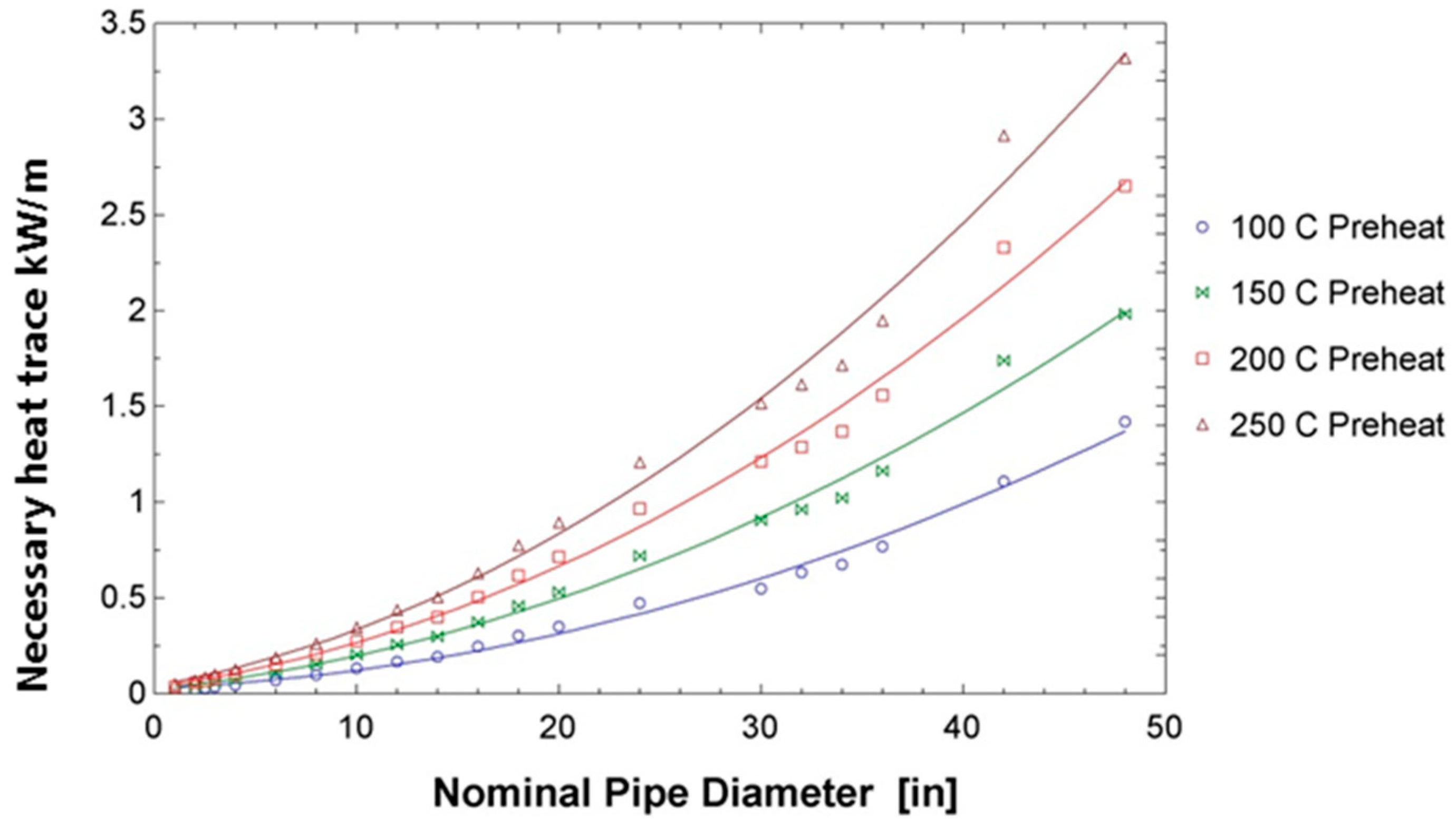
First, results for the pre-heating regime were generated. Based on the pipe diameter and the required pre-heat temperature, the heat trace system can be calculated. The results presented in Figure 9 show that the heat trace requirements increase with the nominal pipe diameter as expected. Some variation is observed based on the non-linearity of schedule 40 pipe thicknesses.

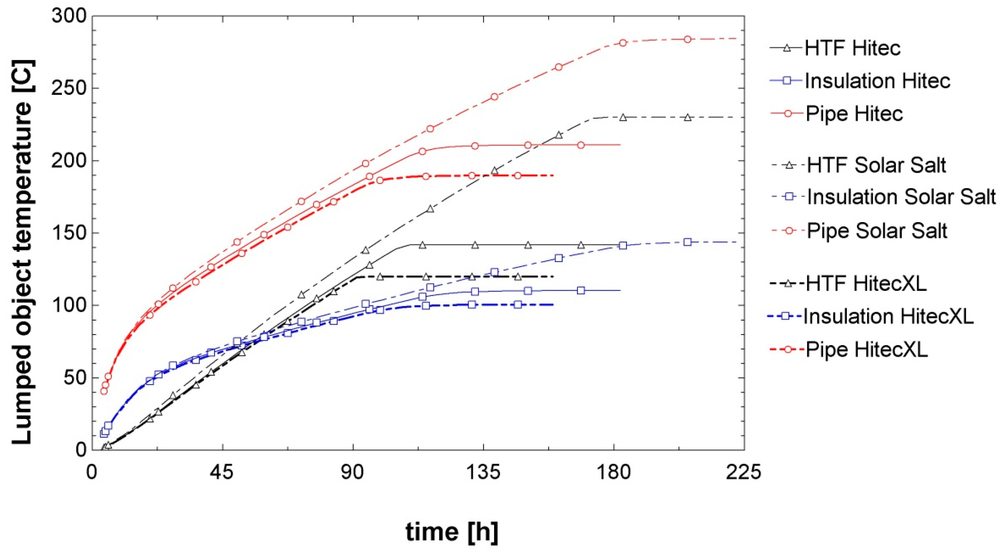
The results in Figure 10 show the transient behaviour of the system during a freeze recovery. As the salt HTF begins to melt, the temperature value reaches the constant value of the phase change temperature. The figure shows the temperature transients for the pipe, insulation, and internal salt during the freeze recovery process for each candidate salt using a heat trace system. This is designed for an 8 h preheat to 100 °C for a 48” pipe, with a wind speed of 5 m/s and an ambient temperature of 15 °C. The line type denotes the HTF type and the colour/symbol denotes the system component. The melting process is finished when the lines stop.

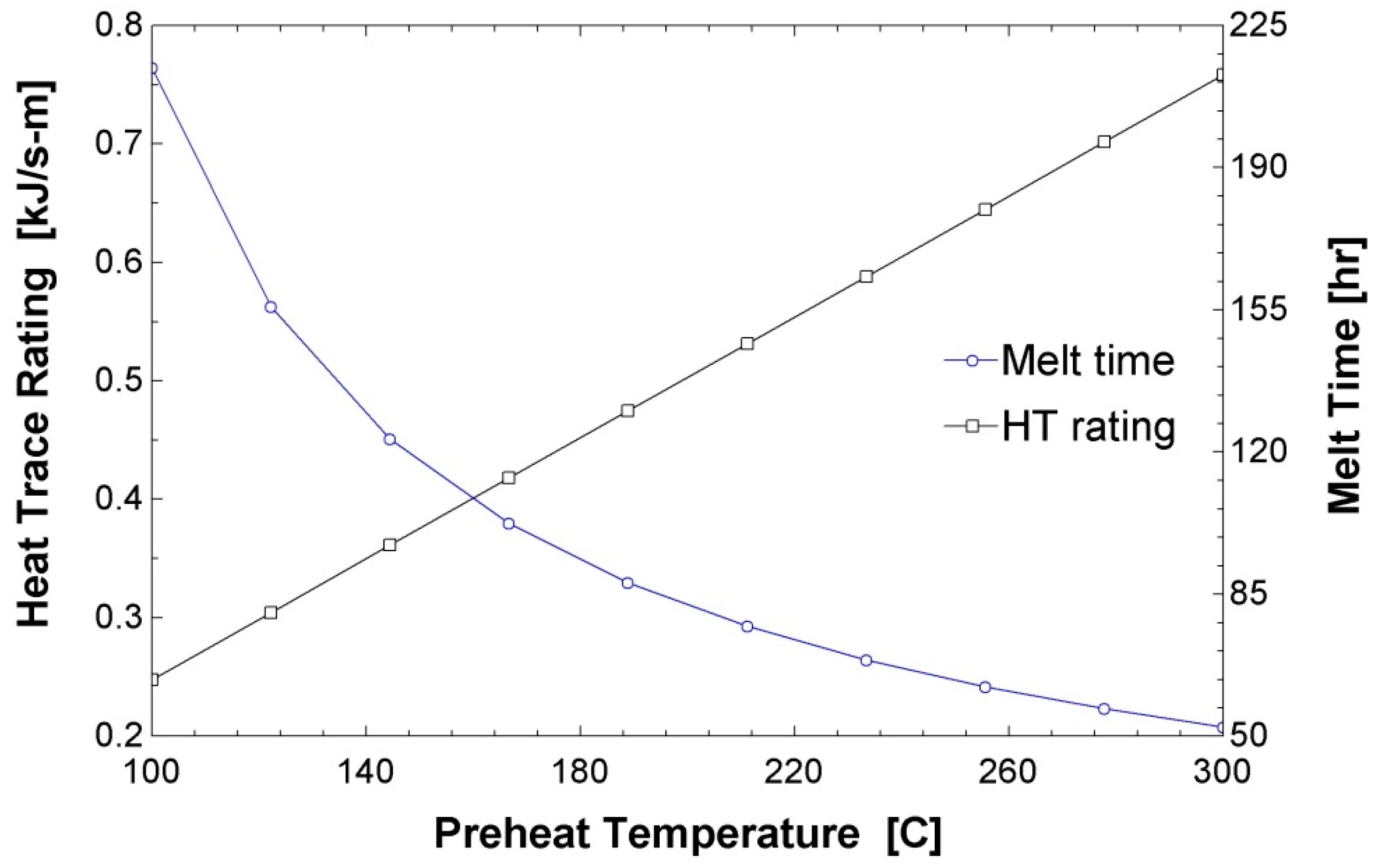
Further investigation of the melting time was performed. Figure 11 shows that because the model first sizes the system based on a user specified preheating time and then solves for melting transients, the melting rate is adversely affected by the initial preheating temperature that is specified per HTF. The system heat trace rating is proportional to the specified preheating temperature per each HTF, where the system melting performance drops off significantly as the specified preheating temperature is decreased.

The model has been integrated with the preliminary field pipe sizing model to generate the total heat trace system required for a molten salt HTF plant. The total model generates the optimal diameters for each pipe segment. Then, using a subprogram, the number of heat trace cables is calculated for each segment to satisfy the preheating requirements. The largest available heat trace cables output 0.05 W/m at their maximum operation. Since the code generates the required heating in W/m as well, it is a division criterion to arrive at the total number of heat trace cables for any pipe section. Multiplying by the length of each segment, we arrive at the total length of heat trace cable required in the plant, where redundant heat trace cables are added to the system to allow for fast recovery from failed heat trace cables. Redundant cables are calculated so that there are always at least 50% more cables then necessary. If the number of cables on the pipe is less than four, then two redundant cables are added. The redundant cables are not wired and are only connected if a cable on the same pipe fails. The total number of cables, redundant and wired, can be used to generate the total heat trace system cost.

The results in

Table 2. Plant heat trace specifications for a HiTec XL-based plant with 388 collector loops.

Nominal Pipe Size (in)	Total Heat Trace Power Cold Pipes (kW)	Total Heat Trace Power Hot Pipes (kW)	Total Heat Trace Cable Length Cold Pipes (m)	Total Heat Trace Cable Length Hot Pipes (m)
4	64	62	904	904
6	355	331	4250	4250
8	1107	1045	11,748	11,748
10	1921	1828	20,656	20,656
12	2349	2231	22,464	22,464
16	550	529	5684	4872
18	676	652	6902	6090
Plant Total	7022	6678	72,608	70,984
	13,700		143,592

,

Table 3. Plant heat trace specifications for a Solar Salt-based plant with 388 collector loops.

Nominal Pipe Size (in)	Total Heat Trace Power Cold Pipes (kW)	Total Heat Trace Power Hot Pipes (kW)	Total Heat Trace Cable Length Cold Pipes (m)	Total Heat Trace Cable Length Hot Pipes (m)
4	88	86	1248	1248
6	391	365	4680	4680
8	1138	1074	12,072	12,072
10	1857	1767	19,968	19,968
12	2217	2106	21,204	21,204
16	550	529	5684	4872
18	676	652	6902	6090
Plant Total	6917	6578	71,758	70,134
	13,496		141,892

,

Table 4. Plant heat trace specifications for a HiTec-based plant with 388 collector loops.

Nominal Pipe Size (in)	Total Heat Trace Power Cold Pipes (kW)	Total Heat Trace Power Hot Pipes (kW)	Total Heat Trace Cable Length Cold Pipes (m)	Total Heat Trace Cable Length Hot Pipes (m)
3	16	15	280	280
4	68	66	968	968
6	391	365	4680	4680
8	1138	1074	12,072	12,072
10	1857	1767	19,968	19,968
12	2217	2106	21,204	21,204
16	550	529	5684	4872
18	676	652	6902	6090
Plant Total	6913	6574	71,758	70,134
	13,488		141,892

and

Table 5. Comparison of heat trace systems for three candidate salts for a plant with 388 collector loops.

Salt	Total Heat Trace Power (kW)	Total Heat Trace Cable Length (m)
HiTec XL	13,700	143,592
Solar Salt	13,496	141,892
HiTec	13,488	141,892

show that HiTec and Solar Salt both require 141,892 m of heat trace cable, while HiTec XL requires 143,592 m. The values for HiTec and Solar Salt are the same because the heat trace cables come in discrete numbers and rounding causes the slight difference in required power to be lost. HiTec XL heat trace system requirements are larger because the pipe sizes for a HiTec XL based system were found to be slightly larger than the other two salts. Heat trace system sizes are a function of the pipe sizes and the HTF properties, but, because pipe sizes are only a function of HTF properties, the heat trace system size can also be considered a function of HTF properties.

4.2. Results and Discussion for the Impedance System

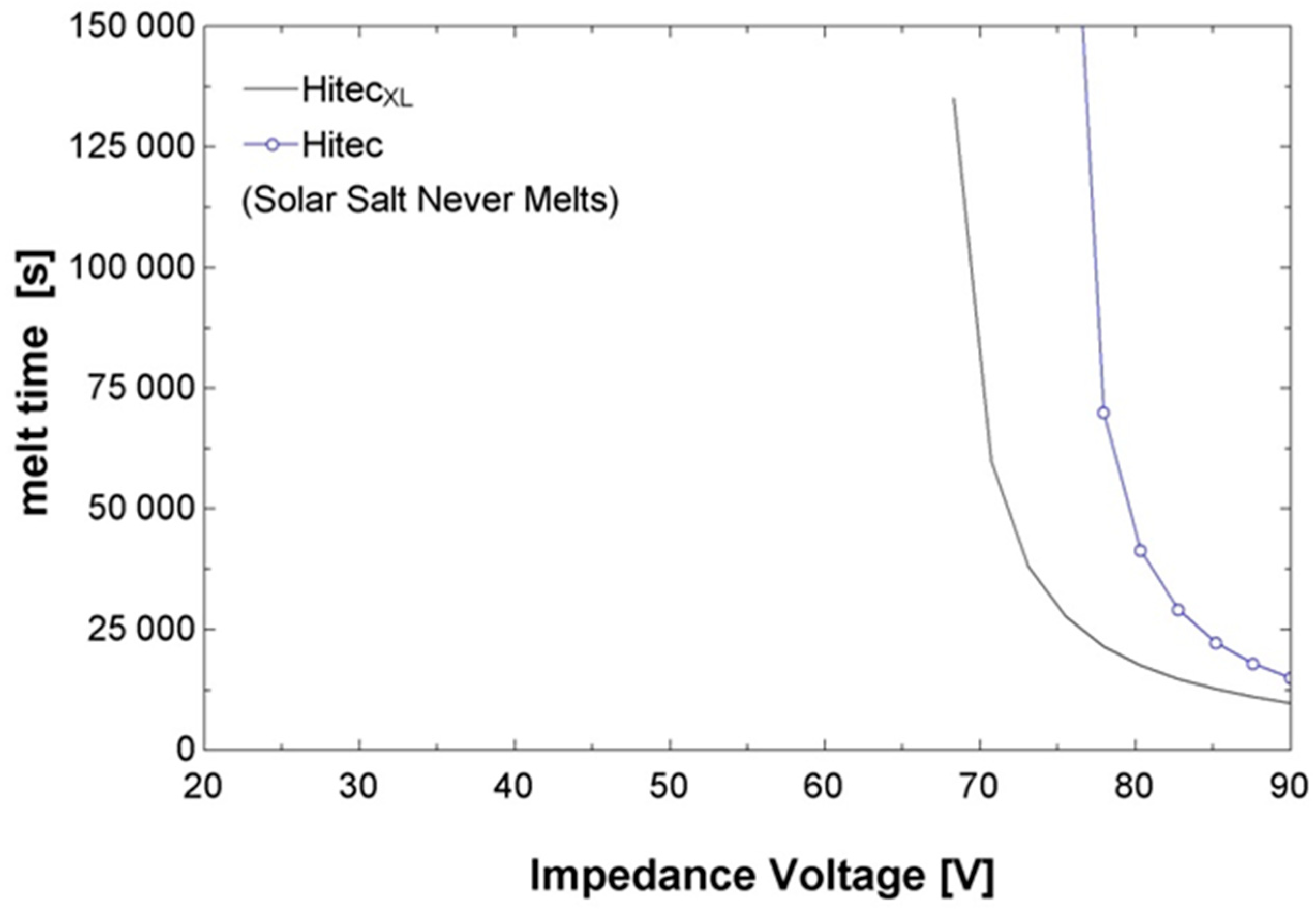
What is most significant to the sizing of an impedance heating system is its performance in off design conditions, such as during the night or in times of low solar irradiation. Figure 12 shows the melting time at different impedance voltages for a nominal system. An asymptotic behaviour is seen, where the salt is not able to be melted until a certain voltage threshold is reached. The effect of the high melting temperature of Solar Salt is observed on its ability to be melted. A much higher impedance voltage is needed to overcome the higher levels of heat loss due to the higher required melting temperature.

Figure 13 shows the melting time for a system with a compromised vacuum. Very high voltages are necessary to melt HiTec or HiTec XL, and no voltage under 90 volts can overcome the heat loss. The IEEE Std 844-2000 (IEEE Recommended Practice for Electrical Impedance, Induction, and Skin Effect Heating of Pipelines and Vessels) standard voltage limit of 80 volts hinders meeting this standard while still melting any of the salt options. This suggests that multiple transformers may be needed per solar collector assembly (SCA) to supply enough energy to cause melting.

Tubes with no glazing were also studied, but no voltages were found that were capable of melting any of the salt options. For this reason, no graph is presented.

The effect of wind speed on melting time was also considered. However, it was found that wind speeds of even 15 m/s had little (less the 5%) effect on the melting time. For the nominal tube, melting is possible for any operational wind condition. For a tube with broken or no glazing, melting is difficult or impossible without solar radiation.

The material of the absorber was also analysed in this study. Currently ASTM 310 stainless steel is proposed. This material offers an appropriate resistivity value, but it could be improved. Since impedance heating is dependent on the square of current to determine power, materials with lower resistivities tend to perform better as heat generators. An analogy is shown below to help understand this trend. Given a large battery with two terminals, if the terminals are connected by something with high resistivity, like wood or plastic, no heat is generated. However, if the cables are connected to a material with low resistivity like copper, the wire will glow and generate large amounts of heat.

Figure 14 shows the melting time relative to the current system configurations for various stainless steel types. A 10–15% decrease in the melting time can be achieved by switching to 201 or 301 stainless steel. While this is an improvement, this change does not improve the overall situation significantly.

The goal of the model development was to design the system necessary to supply adequate impedance heating to recover from a freeze event. To do this, an operational target was developed. The metrics used in the target are summarized in

Table 6. Operation target metrics.

Metric	Target
Melting time	1 day
Worst case configuration	Lost vacuum

.

One day was chosen as a melting time as a standard time from a commercial plant. Lost vacuum was chosen as the worst case because it is assumed that any collectors with broken envelopes would be repaired prior to melting. On the other hand, lost vacuums are not easy to diagnose and are often only replaced at infrequent intervals. Therefore, during a freeze event, some tubes with lost vacuums would need to be melted.

Impedance heating provides a constant heat input along the entire length of the pipe. Furthermore, axial thermal conduction in the pipe and salt is minimal. This allows for each heat collection element (HCE) to be modelled as an island. That is, a HCE with no vacuum will melt at the same rate, no matter whether it is surrounded by tubes with vacuums intact, with no vacuum, or with no glazing. We assume that in every loop there will be at least one HCE with no vacuum, constraining our melting time to the melting time of an HCE with no vacuum.

A system using each salt was analysed for two electrical configurations: One transformer per SCA and two transformers per SCA. For the one transformer setup a connection cable length of 80 m was used. For the two-transformer setup 40 m was used. Figure 15 shows a design layout for a system with one transformer per SCA. The cable lengths are shown with the arrow tipped lines going to and from the transformer. The necessary voltage to reach the target conditions was calculated assuming no solar radiation. These results are tabulated in

Table 7. Necessary electrical system characteristics to meet the target condition of a one-day melting time for a tube with a compromised vacuum. NA represents that no American wire gauge (AWG) rating is sufficient.

Parameter	HiTec XL	HiTec	Solar Salt
1 transformer per SCA
Voltage (V)	69.37	77.26	104
Current (A)	260.2	289.8	390.1
Connector Area (mm2)	64,937	280,108	infinity
Connector Gauge (AWG)	2	n.a.	n.a.
2 transformers per SCA
Voltage (V)	34.69	38.63	52
Current (A)	260.2	289.8	390.1
Connector Area (mm2)	7616	9289	18,479
Cable Gauge (AWG)	11	11	7

. HiTec and Solar Salt systems will need to have two transformers per SCA.

Finally, the total melting time of the system was investigated. It was not considered that the whole field is melted simultaneously, so as not to penalize the cost of the transformers that feed the impedance currents. Different cases of loop simultaneity were considered. The number of loops capable of melting simultaneously was the parameter to optimize. Based on the cost of the DC conductor necessary to feed each loop and the complexity of the utility of switching the plant from a 240 MW source to a 150 MW sink, the actual number was estimated to be around 10. This results in total plant melting times from 100 to 300 days. This represents a significant financial penalty for freezing.

5. Conclusions

Parabolic trough collector (PTC) technology with thermal oil as the HTF is currently the most mature solar technology that is implemented at commercial scale. The use of molten salts as HTF has the advantage of being able to work at higher temperature to increase plant efficiency, and the disadvantage of the potential freezing of the HTF in pipes and components. Two methods of freeze recovery needed in this design have been developed to evaluate the technical feasibility of molten salt in PTC systems. A model of heat tracing in pipes and components, and a model of impedance melting in the solar field has been developed in this paper to compare the freezing protection system in three molten salts mixtures, namely Solar Salts, Hitec and Hitec XL.

In the heat tracing model, all piping included in the heat trace system was heated using a mineral insulted (MI) cable. This is the only type of heat trace cable that can withstand exposure temperatures over 250 °C. Mineral wool thermal insulation with an aluminium jacket was used on all traced piping. Mineral wool insulation was used on valve bodies and bonnets with removable blankets on the actuators. The heat tracing model has been created to size the heat tracing system for any pipe. In addition, the model has been applied to the overall pipe sizing and costing model to make future system cost estimations more accurate.

The model has evaluated the recovery after a freezing event, obtaining that the melting times are acceptable for all pipe diameters proposed in the study. The result of the model also shows how HiTec salt requires less heat trace power in its operation. When evaluating the three fluids, it is concluded that the recovery from freezing in a molten salt plant is possible. The threat of system wide HTF freeze events does not invalidate the concept of molten salt HTFs.

In the impedance model, the receiver tubes were heated with impedance heating, which consisted of a standalone panel and transformer for each collector. Each impedance heating system was a mid-point system to avoid the need for electrical isolation between the receiver tubes and adjacent piping.

The impedance heating model has analysed the performance under off-design conditions (tubes with lost vacuum and high wind losses), showing the increase in the melting time for tubes with a compromised vacuum. This requires working with two SCA transformers for HiTec and Solar Salt. Additionally, more than 100 days will be needed to completely melt a fully frozen solar field.

Even when the melting times involved are not ideal, the reliability of an impedance-based recovery system is high and, as such, freeze events do not stand in the way of future work on molten salt HTF systems.

The models developed show that both systems are technically feasible, since the plant may recover from a freezing event in all studied cases, although the recovery times considerably penalize the performance of the plant. Therefore, an economical detailed study including capital expenditure and operational expenditure (CAPEX and OPEX) is necessary to see which system is the best for a commercial plant.

References

1. International Energy Agency (IEA). Medium-Term Renewable Energy Market Report; International Energy Agency (IEA): Paris, France, 2015. [Google Scholar]
2. International Energy Agency (IEA). Technology Roadmap Solar Thermal Electricity; International Energy Agency (IEA): Paris, France, 2014. [Google Scholar]
3. Siva, V.; Kaushik, S.; Ranjan, K.; Tyagic, S. State-of-the-art of solar thermal power plants: A review. Renew. Sustain. Energy Rev. 2013, 27, 258–273. [Google Scholar] [CrossRef]
4. Zhanga, H.; Baeyens, J.; Degréve, J. Concentrated solar power plants: Review and design methodology. Renew. Sustain. Energy Rev. 2013, 22, 466–481. [Google Scholar] [CrossRef]
5. Description, Solar Paces Website CSP Technology. Available online: http://www.solarpaces.org/ (accessed on 10 September 2017).
6. Office of Energy Efficiency & Renewable, Energy. Available online: http://energy.gov/eere/energybasics/articles/linear-concentrator-system-basicsconcentrating-solar-power (accessed on 10 September 2017).
7. Vignarooban, K.; Xu, X.; Arvay, A.; Hsu, K.; Kannan, A. Heat transfer fluids for concentrating solar power systems—A review. Appl. Energy 2015, 146, 383–396. [Google Scholar] [CrossRef]
8. Benoit, H.; Spreafico, D.; Gauthier, D.; Flamant, G. Review of heat transfer fluid in tube-recievers used in concentrating solar thermal systems: Properties and heat transfer coefficients. Renew. Sustain. Energy Rev. 2016, 55, 298–315. [Google Scholar] [CrossRef]
9. Turchi, C.S.; Vidal, J.; Bauer, M. Molten salt power towers operating at 600–650 °C: Salt selection and cost benefits. Sol. Energy 2018, 164, 28–46. [Google Scholar] [CrossRef]
10. Zarza, E. Innovative working fluids for parabolic trough collectors. In Advances in Concentrating Solar Thermal Research and Technology; Woodhead Publishing: Sawston, UK, 2017; pp. 75–106. [Google Scholar]
11. Fuqiang, W.; Ziming, F.; Jianyu, T.; Yuan, Y.; Yong, S.; Linhu, L. Progress in concentrated solar power technology with parabolic trough collector system: A comprehensive review. Renew. Sustain. Energy Rev. 2017, 79, 1314–1328. [Google Scholar] [CrossRef]
12. Heidsieca, S.; Dörrich, S.; Weidner, R.; Rieger, B. Branched siloxanes as possible new heat transfer fluids for application in parabolic through solar thermal power plants. Sol. Energy Mater. Sol. Cells 2017, 161, 278–284. [Google Scholar] [CrossRef]
13. Zhao, Y.T.C. A review of solar collectors and thermal energy storage in solar thermal applications. Appl. Energy 2013, 104, 538–553. [Google Scholar]
14. Moens, L.; Blake, D. Mechanism of hydrogen formation in solar parabolic trough receivers. J. Sol. Energy Eng. 2010, 132, 031006. [Google Scholar] [CrossRef]
15. Kearney, D.; Herrmann, U.; Nava, P.; Mahoney, R.; Pacheco, J.; Cable, R.; Potrovitza, N.; Blake, D.; Price, H. Assessment of a molten salt heat transfer fluid in a parabolic trough solar field. J. Sol. Energy Eng. 2003, 125, 170–176. [Google Scholar] [CrossRef]
16. Pitz-Paal, R.; Dersch, J.; Milow, B. European Concentrated Solar Thermal Road-Mapping (ECOSTAR): Roadmap Document; German Areospace Center (DLR): Cologne, Germany, 2005. [Google Scholar]
17. Blake, D.; Moens, L.; Hale, H.P.M.J.; Kearney, D.; Herrmann, U. Proceedings of the 11th SolarPACES International Symposium on Concentrated Solar Power and Chemical Energy Technologie, Proceedings of the SolarPACES 2002, Zurich, Switzerland, 2002; Elsevier: Amsterdam, The Netherlands, 2002. [Google Scholar]
18. Fernández, A.; Galleguillos, H.; Fuentealba, E. Thermal characterization of HITEC molten salt for energy storage in solar linear concentrated technology. J. Therm. Anal. Calorim. 2015, 122, 3–9. [Google Scholar] [CrossRef]
19. Li, C.-J.; Li, P.; Wang, K.; Molina, E.E. Survey of Properties of Key Single and Mixture Halide Salts for Potential Application as High Temperature Heat Transfer Fluids for Potential Application as High Temperature Heat Transfer Fluids for Concentrated Solar Thermal Power Systems. AIMS Energy 2014, 2, 133–157. [Google Scholar] [CrossRef]
20. Flamant, G.; Benoit, H. SFERA II 2014–2017, Summer School, 25–27 June 2014. Available online: https://sfera2.sollab.eu/uploads/images/networking/SFERA%20SUMMER%20SCHOOL%202014%20-%20PRESENTATIONS/Overview%20Heat%20Transfer%20Fluid%20-%20Gilles%20Flamant.pdf (accessed on 10 September 2017).
21. Sau, S.; Corsaro, N.; Crescenzi, T.; Liberatore, R.; Licoccia, S.; Russo, V.; Tarquini, P.; Tizzoni, A. Techno-economic comparison between CSP plants presenting two different heat transfer fluids. Appl. Energy 2016, 168, 96–109. [Google Scholar] [CrossRef]
22. Kernay, D.; Kelly, B.; Herrmann, U.; Cable, R.; Pacheco, J.; Mahoney, R.; Priece, H.; Blake, D.; Nava, P.; Potrovitza, N. Engineering aspects of a molten salt heat transfer fluid in a trough solar field. Energy 2004, 29, 861–870. [Google Scholar] [CrossRef]
23. Prieto, C.; Osuna, R.; Fernandez, A.I.; Cabeza, L.F. Thermal storage in a MWscale. Molten salt solar thermal pilot facility: Plant description and commissioning experiences. Renew. Energy 2016, 99, 852–866. [Google Scholar] [CrossRef]
24. Gil, A.; Medrano, M.; Martorell, I.; Lazaro, A.; Dolado, P.; Zalba, B.; Cabeza, L. State of the art on high temperature for power generation. Part 1 Concepts, materials and modellization. Renew. Sustain. Energy Rev. 2010, 14, 31–55. [Google Scholar] [CrossRef]
25. Yılmaz, İ.H.; Mwesigye, A. Modeling, simulation and performance analysis of parabolic trough solar collectors: A comprehensive review. Appl. Energy 2018, 225, 135–174. [Google Scholar] [CrossRef]
26. Bergman, T.L.; Incropera, F.P.; DeWitt, D.P.; Lavine, A.S. Fundamentals of Heat and Mass Transfer; John Wiley & Sons, Inc.: Hoboken, NJ, USA, 2007. [Google Scholar]
27. Indeeco. Available online: https://indeeco.com/files/6514/7948/7711/Impedance_Heating_Systems.pdf (accessed on 24 July 2018).
28. Forristall, R. Heat Transfer Analysis and Modeling of a Parabolic Trough Solar Receiver Implemented in Engineering Equation Solver; No. NREL/TP-550-34169; National Renewable Energy Lab.: Golden, CO, USA, 2003. [Google Scholar]
Figure 1. Main concentrated solar power (CSP) technologies [2].
Energies 12 02340 g001
Figure 2. Several mounting configurations for heat trace cables based on the type of pipe element (valve, joint, or pipe).
Energies 12 02340 g002
Figure 3. Schematic and heat transfer mechanisms through insulated pipe.
Energies 12 02340 g003
Figure 4. Circuit schematic of pipe heat transfer.
Energies 12 02340 g004
Figure 5. Thermal networks used for modelling melting (left) and preheating (right).
Energies 12 02340 g005
Figure 6. End-point electrical connection (Adapted from [27]).
Energies 12 02340 g006
Figure 7. Mid-point electrical connection (Adapted from [27]).
Energies 12 02340 g007
Figure 8. Updated thermal resistance network for the heat collection element (HCE) thermal losses model. q·i,p = impedance heat generation at thermodynamic centre of pipe wall. q·i,s = impedance heat generation in salt.
Energies 12 02340 g008
Figure 9. Required heat trace systems for different levels of preheating for the full range of schedule 40 piping, with a wind speed of 5 m/s and an ambient temperature of 15 °C.
Energies 12 02340 g009
Figure 10. Temperature transients for the pipe, insulation, and internal salt during the freeze recovery.
Energies 12 02340 g010
Figure 11. Effect of initial preheating temperature on melting time and the heat trace rating for a system with a 48″ pipe using Solar Salt.
Energies 12 02340 g011
Figure 12. Melting time as a function of the total solar collector assembly impedance voltage with the following system configurations: Solar radiation = 0 W/m2, wind speed = 5 m/s, glazing intact, vacuum intact.
Energies 12 02340 g012
Figure 13. Melting time as a function of the total solar collector assembly impedance voltage with the following system configurations: Solar radiation = 0 W/m2, wind speed = 5 m/s, glazing intact, air in annulus at 1 atm, ambient temperature = 15 °C.
Energies 12 02340 g013
Figure 14. Relative melting times for different types of stainless steel based on resistivity.
Energies 12 02340 g014
Figure 15. A design schematic for a system with one transformer per solar collector assembly (SCA), given with one possible voltage and amperage.
Energies 12 02340 g015