Data-Driven Stochastic Scheduling for Energy Integrated Systems

Abstract

As the penetration of intermittent renewable energy increases and unexpected market behaviors continue to occur, new challenges arise for system operators to ensure cost effectiveness while maintaining system reliability under uncertainties. To systematically address these uncertainties and challenges, innovative advanced methods and approaches are needed. Motivated by these, in this paper, we consider an energy integrated system with renewable energy and pumped-storage units involved. In addition, we propose a data-driven risk-averse two-stage stochastic model that considers the features of forbidden zones and dynamic ramping rate limits. This model minimizes the total cost against the worst-case distribution in the confidence set built for an unknown distribution and constructed based on data. Our numerical experiments show how pumped-storage units contribute to the system, how inclusions of the aforementioned two features improve the reliability of the system, and how our proposed data-driven model converges to a risk-neutral model with historical data.

1. Introduction

In the past several years, renewable energy, and in particular, wind power, has maintained an increasing penetration in the power system. For instance, more than 33% of the total electricity consumption served by the California Independent System Operator (CAISO) are provided from renewable energy resources [1]. Nevertheless, due to the usually intermittent nature of wind power, the high penetration of such a renewable energy source fluctuates, leading to a fluctuation in power generation, which involves sophisticated power system operation and creates difficulties for the system to schedule power generation [2]. An example is the duck curve [3], a well-known new pattern of the CAISO demand curve. Therefore, advanced modeling and solutions are needed so that demands can be satisfied while renewable energy is maximally harnessed.

Currently, pumped-storage units are outstanding representatives of power storage devices that can offset the impacts of the aforementioned properties of renewable energy by transferring energy from low-use periods to peak-use periods [4]. Therefore, energy systems that integrate thermal generators, wind farms and pumped-storage units are now becoming a popular research subject, and we refer to this kind of power system as an energy integrated system.

In addition, recently, significant research progress has been achieved to address the uncertainty brought by renewable energy generation [5,6]. Among such studies, stochastic optimization and robust optimization are common approaches to address the aforementioned uncertainty to help improve decision making, since these approaches are suitable for a real-time power system and electricity market [5]. However, stochastic programming requires large quantities of data that are utilized to generate many possible scenarios, and consequently, the model becomes difficult to solve computationally; additionally, if the number of scenarios is limited, a suboptimal solution may be derived. Moreover, robust optimization may lead to conservative dispatch results since it considers the worst case. Therefore, in this paper, we propose a data-driven risk-averse two-stage stochastic model to hedge against uncertainty.

In practice, some thermal generators have forbidden zones due to physical limitations; for example, vibrations may be amplified in certain ranges, which are just called forbidden zones [7]. Therefore, considering that power generation ramps are continuous in real-time operation that power generation in the forbidden zones is thus inevitable, power generation must be within such zones in the shortest possible time in order to minimize damage to the mechanical system [6]. Motivated by this idea, we include generators’ operations within forbidden zones in our proposed model so that the model can more accurately represent the operation system in the real world. Moreover, in real-time operations in ISOs the ramping rates of generators vary in different zones, which means that the ramping rate is dynamic according to the zone of the generator [8]. Therefore, involving dynamic ramping rate limits in the proposed model is crucial to improve the reliability of the system.

1.1. Problem Description

In this paper, we consider the unit commitment (UC) problem in an energy integrated system in which thermal generators, wind farms and pumped-storage units are integrated. In this problem, the renewable energy generation and demands are uncertain, which results in uncertainties in the system that need to be addressed. Moreover, to accurately model the operation of thermal generators, we consider forbidden zones and dynamic ramping rate limits in the proposed model. We aim to study how the pumped-storage units improve the operation of the system, show the effectiveness of our proposed data-driven risk-averse stochastic model in optimizing the operation of the system under uncertainty and present the reliability of the system when forbidden zones and dynamic ramping rate limits are included.

Therefore, we are tasked with constructing a data-driven risk-averse two-stage stochastic model to minimize the total cost of the energy integrated system that includes forbidden zones and dynamic ramping rate limits under uncertainty. Decisions in the UCs and power generation are made at discrete time periods over a finite time horizon. Furthermore, appropriate approaches are adopted to help solve the model efficiently.

1.2. Paper Organization

The remaining parts of this paper are organized as follows. Section 2 reviews the most relevant studies in UCs and the corresponding solution techniques. Section 3.1 introduces the deterministic two-stage model with forbidden zones and dynamic ramping rate limits. Then, Section 3.2 describes how to derive the data-driven risk-averse two-stage stochastic model by introducing constructions of confidence sets with $L_1$ and $L_{\infty }$ norms and introduces how to develop the Benders decomposition algorithm to solve the corresponding model. Section 4 provides computational results and demonstrates the reliability and practicality of our proposed model. Finally, Section 5 concludes this paper.

2. Literature Review

There is a rapidly growing body of literature on power systems that integrate pumped-storage units and wind generation. Functions of pumped-storage units in the power system have been studied in real cases [9,10,11] and their significances are proved, especially their specialists in addressing the uncertainty when the renewable energy is involved in the power system. Furthermore, current studies analyse more details about characteristics of pumped-storage units that play vital roles in addressing the variability and the uncertainty in the power system, for example, their capacities [4,12,13] and allocations [14,15,16]. And detailed solutions of how to optimize two such characteristics of pumped-storage units for achieving a more cost-efficient power system are provided. Although the aforementioned studies present advantages of pumped-storage units in the power system in real cases and offer efficient solutions in how to utilize them in a smart way, they neglect properties of thermal generators in real-time operations, and consequently the systems that they consider cannot be perfectly reliable.

To address the uncertainty in the UC problem, stochastic optimization and robust optimization are two popular traditional optimization-under-uncertainty techniques. Two-stage stochastic frameworks are built for solving UC problems under uncertainty in [17,18]; the former study considers the uncertainty due to wind power output, whereas the latter study investigates the problem when demands are uncertain. Similarly, a two-stage stochastic programming (TSP) approach is applied to address the uncertainty associated with the electricity price in the UC problem [19]. However, even though the aforementioned studies provide significant performances in dealing with their studied issues, problems cannot be solved in the extended form when a large number of scenarios is taken into account. To overcome the obstacle associated with large number of scenarios, Niknam et al. [20] utilize improved teaching–learning-based optimization algorithm and Farzin et al. [21] employ the model predictive control based techniques algorithm. However, their methods cannot work without a predetermined probabilistic distribution of the uncertainty parameters. Actually a predetermined random distribution is necessary when the stochastic optimization approach is adopted to solve the UC problem [22,23]. In addition, robust optimization has been extensively studied to help the power system make better decisions under uncertainties. Some early studies [24,25,26] apply robust optimization techniques in modelling and solving UC problems and demonstrate the effectiveness of robust optimization. However, they all possibly lead to excessively conservative solutions. In order to control the conservatism, Chen et al. [27] configure uncertainty range to cover the uncertainty within each scenario. However, this method requires operators to pick the proper scenario, which is a little bit subjective and may lead to solutions of low accuracy. And Wu et al. [28] employ robust interval optimization algorithm to address uncertainties, which may lead to excessively conservative solutions as the wind power prediction error becomes large. Although the conservatism of robust optimization can also be reduced by adopting the approach of adjusting the budget of uncertainty [29] or utilizing dynamic uncertainty sets [30], there is no systematic method to prioritize the value of budget of uncertainty.

Currently, most studies [31,32,33] focus on a model of traditional thermal generators in a UC problem without taking into account forbidden zones and dynamic ramping rate limits. Even if such two features are included, the corresponding constraints are not reliable enough. For example, forbidden zones in the formulation of the UC are considered in studies [7,34,35], nevertheless, they assume that power generation within forbidden zones is prohibited. However, this assumption is impractical, since the the power generation ramps continuously, which means that power generation within forbidden zones is inevitable. Regarding studies about dynamic ramping rate limits, Li and Shahidehpour [8] consider dynamic ramping rates as stepwise or piecewise functions of generation and include this feature by proposing these functions. However, the constructed models have limitations in imitating the transitions of the ramping rates across different zones (e.g., from a forbidden zone to a normal zone). Based on Li and Shahidehpour [8], Correa-Posada et al. [36] further improve the formulation with dynamic ramping rate limits taken into account by incorporating more realistic cases. Unfortunately, these studies cannot capture the dynamic ramping rate limits accurately, since they do not take into account forbidden zones, which have special requirements [37].

Motivated by these, in this paper, we try to deal with the aforementioned defects, and the main results and contributions are summarized as follows:

• We consider an energy integrated system that integrates thermal generators, wind farms and pumped-storage units. The performances under both deterministic conditions and stochastic conditions show the benefits of employing pumped-storage units that can contribute to hedging against the uncertainty, specifically in decreasing the total costs and the total online time of the generators. Indeed, the internet system considered here enables more reliable and practical operation.
• We establish a data-driven risk-averse two-stage stochastic model, which behaves much better than current traditional stochastic or robust programming models in hedging against uncertainty. We does not need a predetermined distribution of uncertain parameters that traditional stochastic optimization requires. Moreover, the conservativeness level of our model can be simply adjusted based on the number of data samples, which is unavailable in traditional robust optimization. Benefiting from these, we can obtain reliable solutions with less efforts spent in dealing with data and the model’s conservativeness, which increases the computational efficiency of the model.
• We consider a significantly accurate model by including forbidden zones and dynamic ramping rate limits simultaneously through a status transition modeling approach. This formulation performs well in improving the reliability and feasibility of the system.

3. Methodology

In this paper, we construct a data-driven risk-averse two-stage stochastic model with forbidden zones and dynamic ramping rate limits to minimize the total cost of the energy integrated system by aggregating generation decisions and uncertainties in the second-stage problem after determining the UCs and status transitions of the generators in the first-stage problem. By employing a status transition modeling approach, we include the forbidden zones and dynamic ramping rate limits in our proposed model while ensuring that the model is solvable. This model is precisely introduced in Section 3.1 and Section 3.2.

We employ the Monte Carlo simulation method [38] to generate more data based on the historical data that we already have. By utilizing such historical data, we then derive a distributional ambiguity set, a confidence set, for the distributions of uncertain parameters, for example, uncertain demands, and optimize the total cost against the worst-case distribution in this set, leading to a data-driven risk-averse model. The construction of the confidence set is precisely introduced in Section 3.2.2. To address the computational challenge, we employ the Benders decomposition approach to solve the risk-averse two-stage stochastic model [39,40], the details of which are presented in Section 3.2.3.

3.1. Deterministic Model

In this paper, we first construct a model for the energy integrated system considering forbidden zones and dynamic ramping rate limits.

Our goal is to minimize the total cost of the system; therefore, we construct the objective function as follows:

$$\begin{array}{cc}\hfill min& \sum _{k\in \mathcal{G}}\sum _{t=1}^T\left({\mathrm{SU}}^k{u}_t^k+{\mathrm{SD}}^k\left(y_{t-1}^k-y_t^k+u_t^k\right)+{\Phi }_t^k(·)\right)\hfill \end{array}$$

(1)

where the objective function (1) minimizes the start-up/shut-down cost and the operation cost, in which ${\mathrm{SU}}^k$ and ${\mathrm{SD}}^k$ represent the start-up and shut-down costs of generator $k\in \mathcal{G}$, respectively, with $\mathcal{G}$ being the set of generators. Notice here that the operating costs for absorbing or generating power by pumped-storage hydros are usually very low and therefore are not considered in this model. The binary decision variable $u_t^k$ determines if the generator k starts up at time $t\in T$, correspondingly, $u_t^k=1$, or does not start up, $u_t^k=0$, where T represents the total time horizon. The binary decision variable $y_t^k$ determines if the generator k is online at time t, correspondingly, $y_t^k=1$, or offline, $y_y^k=0$. Thus, ${\sum }_{k\in \mathcal{G}}{\sum }_{t=1}^T\left({\mathrm{SU}}^k{u}_t^k+{\mathrm{SD}}^k\left(y_{t-1}^k-y_t^k+u_t^k\right)\right)$ represents the total start-up and shut-down costs. Furthermore, ${\sum }_{k\in \mathcal{G}}{\sum }_{t=1}^T{\Phi }_t^k(·)$ represents the operation cost, which is a quadratic function, i.e., ${\Phi }_t^k\left(x_t^k\right)=a^k{\left(x_t^k\right)}^2+b^k{x}_t^k+c^k{y}_t^k$, that can be approximated by a piecewise linear function with N pieces. For example, following the process introduced in [5], ${\Phi }_t^k\left(x_t^k\right)$ can be represented by the auxiliary variable $f_t^k$ with additional constraints introduced as follows:

$$\begin{array}{c}{f}_t^k\ge (2a^k{\alpha }_n^k+b^k)x_t^k+(c^k-a^k{\alpha }_n^k)y_t^k,\\ \hspace{1em}\forall t\in T,\forall k\in \mathcal{G},\forall n\in [1,N].\end{array}$$

(2)

where ${\alpha }_n^k$ represents the nth break point of the operation range of generator k between its lower bound, ${\underline{C}}_k$, and upper bound, ${\overline{C}}_k$. Decision variables $x_t^k$ denote the amount of power generation of generator k at time t.

Next, we start to build constraints.

$$\begin{array}{c}\sum _{i=t-L^k+1}^t{u}_i^k\le y_t^k,\forall t\in [L^k,T],\forall k\in \mathcal{G},\hfill \end{array}$$

(3)

$$\begin{array}{c}\sum _{i=t-{\ell }^k+1}^t{u}_i^k\le 1-y_{t-{\ell }^k}^k,\forall t\in [{\ell }^k,T],\forall k\in \mathcal{G},\hfill \end{array}$$

(4)

$$\begin{array}{c}-y_{t-1}^k+y_t^k-u_t^k\le 0,\forall t\in [1,T],\forall k\in \mathcal{G},\hfill \end{array}$$

(5)

where Constraints (3) and (4) represent the minimum up and down time limits, respectively. Specifically, (3) constrains generator k to remain online for at least $L^k$ time periods until t if it starts up at time $t-L^k+1$ (i.e., $y_{t-L^k+1}=u_{t-L^k+1}^k=1$). Similarly, (4) constrains generator k to remain offline for at least ${\ell }^k$ time periods until t if it starts up at time $t-{\ell }^k+1$ (i.e., $y_{t-{\ell }^k+1}=u_{t-{\ell }^k+1}^k=1$). Moreover, (5) constrains the relationship between $y_t^k$ and $u_t^k$.

$$\begin{array}{c}{\sum }_{k\in \mathcal{G}}{x}_t^k+{\sum }_{h\in \mathcal{H}}(H_{h,t}^{Out}-H_{h,t}^{In})+{\sum }_{b\in \mathcal{B}}{W}_{b,t}={\sum }_{b\in \mathcal{B}}{d}_{b,t},\forall t\in [1,T],\hfill \end{array}$$

(6)

$$\begin{array}{c}-C_m\le {\sum }_{b\in \mathcal{B}}{K}_m^b\left({\sum }_{k\in {\mathcal{G}}_b}{x}_t^k+{\sum }_{h\in {\mathcal{H}}_b}(H_{h,t}^{Out}-H_{h,t}^{In})+W_{b,t}-d_{b,t}\right)\le C_m,\forall t\in [1,T],\forall m\in \mathcal{M},\hfill \end{array}$$

(7)

where (6) is the load balance constraint and (7) constrains the capacity limits of each transfer line m. In these two constraints, the decision variables $H_{h,t}^{Out}$ and $H_{h,t}^{In}$ represent the amount of electricity generated and absorbed by the pumped-storage unit h at time t, respectively, where $\mathcal{B}$ represents the set of buses, $\mathcal{G}$ means the set of thermal generators and $\mathcal{H}$ denotes the set of pumped-storage units in the system. Moreover, the random parameters $W_{b,t}$ and $d_{b,t}$ denote the random amount of wind power generation and electricity demands at bus b at time t, respectively. The certain parameter $K_m^b$ denotes the line flow distribution factor for transmission line m at bus b, and $C_m$ represents the transmission capacity of line $m\in \mathcal{M}$, where $\mathcal{M}$ denotes the set of lines in the system. In addition, ${\mathcal{G}}_b$ and ${\mathcal{H}}_b$ mean the set of thermal generators and pumped-storage units at bus b, respectively.

$$\begin{array}{c}{s}_{h,t}=s_{h,t-1}+{\eta }_1{H}_{h,t}^{In}-H_{h,t}^{Out}/{\eta }_2,\forall h\in \mathcal{H},\forall t\in [1,T],\hfill \end{array}$$

(8)

$$\begin{array}{c}{L}^{In}\le H_{h,t}^{In}\le U^{In},\forall h\in \mathcal{H},\forall t\in [1,T],\hfill \end{array}$$

(9)

$$\begin{array}{c}{L}^{Out}\le H_{h,t}^{Out}\le U^{Out},\forall h\in \mathcal{H},\forall t\in [1,T],\hfill \end{array}$$

(10)

$$\begin{array}{c}{s}_{h,0}=S_0,\forall h\in \mathcal{H},\hfill \end{array}$$

(11)

$$\begin{array}{c}{s}_{h,T}=S_T,\forall h\in \mathcal{H},\hfill \end{array}$$

(12)

where (8) are hydro storage balance constraints in which the variables $s_{h,t}$ determine the water reserve storage of the pumped-storage unit h at time t and the parameters ${\eta }_1$ and ${\eta }_2$ illustrate the efficiencies of the absorbing and generating cycles of the pumped-storage units, respectively. In addition, the Constraints (9) and (10) determine the lower and upper bounds of the electricity absorbed, represented by $L^{In}$ and $U^{In}$, and the electricity generated, represented by $L^{Out}$ and $U^{Out}$, by the pumped-storage units, respectively. The Constraints (11) and (12) define the initial and final water storage levels, $S_0$ and $S_T$, respectively, for the pumped-storage units.

After constructing the basic constraints for the thermal generators, wind farms and pumped-storage units, we next focus on the constraints for the forbidden zones and dynamic ramping rate limits.

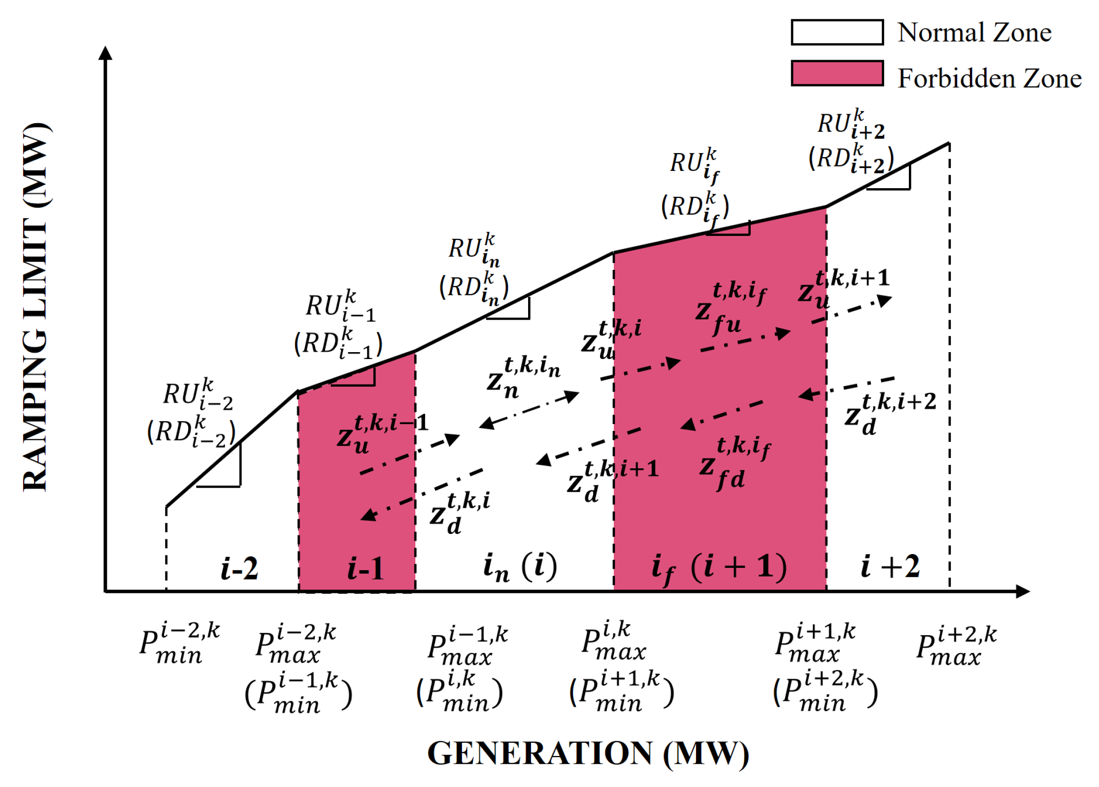
For the relevant constraints, we first introduce some binary decision variables (represented by directed lines) defined to represent the status transitions of the generators among different zones and dynamic ramping rate limits in Figure 1.

As shown in Figure 1, we define a binary variable for each directed dashed line to indicate whether this line is active or not, which reflects the transition status of the generator. If the line is active, it indicates that the corresponding generator changes its status following that directed dashed line. Specifically, we define the binary variable $z_u^{t,k,i}$ to represent whether the transition status of generator k at time t is from zone i to zone $i+1$. If it is, $z_u^{t,k,i}=1$; otherwise, $z_u^{t,k,i}=0$. Similarly, we define the binary variable $z_d^{t,k,i}$ to represent whether the transition status of generator k at time t is from zone i to zone $i-1$. If it is, $z_d^{t,k,i}=1$; otherwise, $z_d^{t,k,i}=0$. In addition, we define the binary variables $z_{fu}^{t,k,i_f}$ and $z_{fd}^{t,k,i_f}$ to represent if the transition of generator k is from forbidden zone $i_f$ to forbidden zone $i_f$ ramping up and ramping down at time t, respectively. We also define the binary variable $z_n^{t,k,i_n}$ to represent if the transition is from normal zone $i_n$ to normal zone $i_n$, regardless of the ramping directions.

In summary, we can divide such binary variables into two types: one type for transitions across different zones (e.g., $z_u^{t,k,i}$ and $z_d^{t,k,i}$) and another type for transitions within one zone (e.g., $z_n^{t,k,i_n}$, $z_{fu}^{t,k,i_f}$ and $z_{fd}^{t,k,i_f}$).

The dynamic ramping rate limits are also presented in Figure 1. Different zones, for instance, normal zone i and forbidden zone $i+1$, have corresponding ramping rate limits that are different, and we define the ramping up and down rates of generator k in zone i as $R{U}_i^k$ and $R{D}_i^k$, respectively, which are equal. Moreover, we define the parameters $P_{min}^{i,k}$ and $P_{max}^{i,k}$ as the minimal and maximal generation outputs of generator k in zone i, respectively.

Based on these definitions, we have following constraints:

$$\begin{array}{c}{z}_n^{t,k,i_n}+z_u^{t,k,i_n-1}+z_d^{t,k,i_n+1}=z_u^{t+1,k,i_n}+z_n^{t+1,k,i_n}+z_d^{t+1,k,i_n},\forall t\in [1,T],\forall i_n\in {\mathcal{N}}_k,\forall k\in \mathcal{G},\hfill \end{array}$$

(13)

$$\begin{array}{cc}\hfill z_{fu}^{t,k,i_f}& +z_{fd}^{t,k,i_f}+z_u^{t,k,i_f-1}+z_d^{t,k,i_f+1}\hfill \\ & =z_u^{t+1,k,i_f}+z_{fu}^{t+1,k,i_f}+z_{fd}^{t+1,k,i_f}+z_d^{t+1,k,i_f},\forall t\in [1,T],\forall i_f\in {\mathcal{F}}_k,\forall k\in \mathcal{G},\hfill \end{array}$$

(14)

where Constraints (13) and (14) ensure that if the generator enters the normal zone $i_n\in {\mathcal{N}}_k$, in which ${\mathcal{N}}_k$ denotes the set of normal zones, or the forbidden zone $i_f\in {\mathcal{F}}_k$, in which ${\mathcal{F}}_k$ means the set of forbidden zones, from any other zones at time t, then at the next time $t+1$ it has to stay within the normal zone $i_n$ or the forbidden zone $i_f$, respectively, or leave to some other possible zone.

$$\begin{array}{c}{\sum }_{i_n\in {\mathcal{N}}_k}\left(z_n^{t,k,i_n}+z_u^{t,k,i_n-1}+z_d^{t,k,i_n+1}\right)\hfill \\ +{\sum }_{i_f\in {\mathcal{F}}_k}\left(z_{fu}^{t,k,i_f}+z_{fd}^{t,k,i_f}+z_u^{t,k,i_f-1}+z_d^{t,k,i_f+1}\right)=y_t^k,\forall t\in [1,T],\forall k\in \mathcal{G},\hfill \end{array}$$

(15)

where Constraints (15) describe the relationship between the online/offline status and the transition status. For example, if generator k at time t is offline ($y_t^k=0$), none of the transition statuses of the generator would be active.

$$\begin{array}{c}{z}_{fu}^{t+1,k,i_f}+z_u^{t+1,k,i_f}\ge z_u^{t,k,i_f-1}+z_{fu}^{t,k,i_f},\forall t\in [1,T],\forall i_f\in {\mathcal{F}}_k,\forall k\in \mathcal{G},\hfill \end{array}$$

(16)

$$\begin{array}{c}{z}_{fd}^{t+1,k,i_f}+z_d^{t+1,k,i_f}\ge z_d^{t,k,i_f+1}+z_{fd}^{t,k,i_f},\forall t\in [1,T],\forall i_f\in {\mathcal{F}}_k,\forall k\in \mathcal{G},\hfill \end{array}$$

(17)

where Constraint (16) and (17) restrict the generator’s operations within the forbidden zones by enforcing the transition direction. Specifically, (16) means that if a generator has an up-transition process at time t in which it ramps up in forbidden zone $i_f$ or enters this zone from zone $i_f-1$, then at time $t+1$ it has to maintain an up-transition process, for instance, by continually ramping up in the forbidden zone $i_f$ or going up to zone $i_f+1$. Similarly, Constraints (17) describe the down-transition process.

$$\begin{array}{c}{x}_t^k\le {\sum }_{i_n\in {\mathcal{N}}_k}\left(z_n^{t,k,i_n}+z_u^{t,k,i_n-1}+z_d^{t,k,i_n+1}\right)P_{max}^{i_n,k}+\hfill \\ {\sum }_{i_f\in {\mathcal{F}}_k}\left(z_{fu}^{t,k,i_f}+z_{fd}^{t,k,i_f}+z_u^{t,k,i_f-1}+z_d^{t,k,i_f+1}\right)P_{max}^{i_f,k},\forall t\in [1,T],\forall k\in \mathcal{G},\hfill \end{array}$$

(18)

$$\begin{array}{c}{x}_t^k\ge {\sum }_{i_n\in {\mathcal{N}}_k}\left(z_n^{t,k,i_n}+z_u^{t,k,i_n-1}+z_d^{t,k,i_n+1}\right)P_{min}^{i_n,k}+\hfill \\ {\sum }_{i_f\in {\mathcal{F}}_k}\left(z_{fu}^{t,k,i_f}+z_{fd}^{t,k,i_f}+z_u^{t,k,i_f-1}+z_d^{t,k,i_f+1}\right)P_{min}^{i_f,k},\forall t\in [1,T],\forall k\in \mathcal{G},\hfill \end{array}$$

(19)

where Constraints (18) and (19) restrict the lower and upper generation bounds of generator k at time t.

$$\begin{array}{c}{x}_{t+1}^k-x_t^k\le {RU}_{i_n}^k\delta z_n^{t+1,k,i_n}+max\{{RU}_{max}^k\delta ,{\overline{V}}^k\}\left(1-z_n^{t+1,k,i_n}\right),\forall i_n\in {\mathcal{N}}_k,\forall t\in [1,T],\forall k\in \mathcal{G},\hfill \end{array}$$

(20)

$$\begin{array}{c}{x}_t^k-x_{t+1}^k\le {\mathrm{RD}}_{i_n}^k\delta z_n^{t+1,k,i_n}+max\left\{{\mathrm{RD}}_{max}^k\delta ,{\overline{V}}^k\right\}\left(1-z_n^{t+1,k,i_n}\right),\forall i_n\in {\mathcal{N}}_k,\forall t\in [1,T],\forall k\in \mathcal{G},\hfill \end{array}$$

(21)

$$\begin{array}{c}(x_{t+1}^k-P_{min}^{i+1,k})/{\mathrm{RU}}_{i+1}^k+(P_{max}^{i,k}-x_t^k)/{\mathrm{RU}}_i^k\le z_u^{t+1,k,i}\delta \hfill \\ +max\left\{{\mathrm{RU}}_{max}^k\delta ,{\overline{V}}^k\right\}/min\left\{{\mathrm{RU}}_{i+1}^k,{\mathrm{RU}}_i^k\right\}\left(1-z_u^{t+1,k,i}\right),\forall i\in {\mathcal{Z}}_k,\forall t\in [1,T],\forall k\in \mathcal{G},\hfill \end{array}$$

(22)

$$\begin{array}{c}(x_t^k-P_{min}^{i,k})/{\mathrm{RD}}_i^k+(P_{max}^{i-1,k}-x_{t+1}^k)/{\mathrm{RD}}_{i-1}^k\le z_d^{t+1,k,i}\delta \hfill \\ +max\left\{{\mathrm{RD}}_{max}^k\delta ,{\overline{V}}^k\right\}/min\left\{{\mathrm{RD}}_{i-1}^k,{\mathrm{RD}}_i^k\right\}\left(1-z_d^{t+1,k,i}\right),\forall i\in {\mathcal{Z}}_k,\forall t\in [1,T],\forall k\in \mathcal{G},\hfill \end{array}$$

(23)

where Constraints (20)–(23) describe the dynamic ramping rate limits. Specifically, Constraints (20) and (21) restrict the ramping rate of the generator within the normal zone, and Constraints (22) and (23) illustrate the ramping rate limits across different zones, in which $\delta$ denotes the unit time interval (e.g., 15 min), ${\overline{V}}^k$ is the start-up/shut-down ramping rate of generator k and ${\mathrm{RU}}_{max}^k$ and ${\mathrm{RD}}_{max}^k$ represent the largest ramping up and down rates, respectively, of generator k among all zones.

Constraints (20) work in such a way that if the generator ramps within the normal zone (i.e., $z_n^{t+1,k,i_n}=1$), it has to be restricted by the ramping rate corresponding to the normal zone $i_n$, for instance, ${RU}_{i_n}^k$; otherwise, such constraints become relaxed since $max\{{RU}_{max}^k\delta ,{\overline{V}}^k\}$ is large enough. Constraint (22) enforces the ramping amount if the generator ramps up across different zones (i.e., $z_u^{t+1,k,i}=1$); otherwise, these constraints will also be relaxed. And Constraints (21) and (23) can be analysed in a similar way.

$$\begin{array}{c}{\mathrm{RU}}_{i_f}^k\delta z_{fu}^{t+1,k,i_f}-max\left\{{\mathrm{RU}}_{max}^k\delta ,{\overline{V}}^k\right\}\left(1-z_{fu}^{t+1,k,i_f}\right)\hfill \\ \le x_{t+1}^k-x_t^k\le {\mathrm{RU}}_{i_f}^k\delta z_{fu}^{t+1,k,i_f}+max\left\{{\mathrm{RU}}_{max}^k\delta ,{\overline{V}}^k\right\}\left(1-z_{fu}^{t+1,k,i_f}\right),\forall i_f\in {\mathcal{F}}_k,\forall t,\forall k\in \mathcal{G},\hfill \end{array}$$

(24)

$$\begin{array}{c}{\mathrm{RD}}_{i_f}^k\delta z_{fd}^{t+1,k,i_f}-max\left\{{\mathrm{RD}}_{max}^k\delta ,{\overline{V}}^k\right\}\left(1-z_{fd}^{t+1,k,i_f}\right)\hfill \\ \le x_t^k-x_{t+1}^k\le {\mathrm{RD}}_{i_f}^k\delta z_{fd}^{t+1,k,i_f}+max\left\{{\mathrm{RD}}_{max}^k\delta ,{\overline{V}}^k\right\}\left(1-z_{fd}^{t+1,k,i_f}\right),\forall i_f\in {\mathcal{F}}_k,\forall t,\forall k\in \mathcal{G},\hfill \end{array}$$

(25)

where Constraints (24) and (25) enforce that once the generator enters the forbidden zone, it has to leave with the highest ramping rate, which equals the ramping rate limit of the forbidden zone $i_f$, so that the generator is ensured to remain there in the shortest time.

3.2. Data-Driven Risk-Averse Model

In this section, based on the deterministic model constructed above, we propose a data-driven risk-averse two-stage stochastic model with forbidden zones and dynamic ramping rate limits. Furthermore, we describe how to construct the confidence set and how to employ Benders decomposition algorithm to solve such a two-stage stochastic model.

3.2.1. Risk-Averse Two-Stage Stochastic Model

In the traditional TSP framework, the distribution of random parameters is known which leads to risk-neutral decisions. For example, a set of scenarios, each with a corresponding probability, are given. Nevertheless, in practice, such probabilities are uncertain, which we consider in this paper. Thus, in this paper, we assume that the net load and the renewable generation are uncertain, and for simplicity, the renewable generation is treated as a proportion of uncertain demands, e.g., 30%. Therefore, in this paper, we consider that the net load distribution (denoted by P) is uncertain and ambiguous. However, P can be predefined within a confidence set $\mathcal{D}$ based on the available samples of historical data, the details of which are introduced in Section 3.2.2. In addition, in our risk-averse TSP model, we determine the optimal decisions in UCs and status transitions of the generators in the first stage, and then the details of the amount of power generation of the thermal units and pumped-storage units are decided against the worst-case scenario in the second stage. Therefore, the corresponding data-driven risk-averse TSP model can be built as follows:

$$\begin{array}{cc}\hfill min& {\sum }_{\forall k,t}\left({\mathrm{SU}}^k{u}_t^k+{\mathrm{SD}}^k(y_{t-1}^k-y_t^k+u_t^k)\right)+{max}_{P\in \mathcal{D}}{\mathbb{E}}_P\left[Q(y,u,\xi )\right]\hfill \\ \hfill \mathrm{s}.\mathrm{t}.& \left(3\right)–\left(5\right),\left(13\right)–\left(17\right)\forall t,k.\hfill \end{array}$$

(26)

where ${\mathbb{E}}_P\left[Q(y,u,\xi )\right]$ means the expectation under distribution P, and $Q(y,u,\xi )$ is defined as follows:

$$\begin{array}{cc}Q(y,u,\xi )\hfill & =min{\sum }_{k\in G}{\sum }_{t=1}^T{f}_t^k\left(\xi \right)\hfill \\ & \mathrm{s}.\mathrm{t}.\left(2\right),\left(6\right)–\left(12\right),\left(18\right)–\left(25\right),\mathrm{given}\xi .\hfill \end{array}$$

(27)

where $\xi$ denotes a certain scenario. We define the variable $f_t^k\left(\xi \right)$ as the replacement of the operation costs ${\Phi }_t^k\left(x_t^k\left(\xi \right)\right)$ of generator k at time t under scenario $\xi$. Thus, here the decision variable $x_t^k\left(\xi \right)$ denotes the amount of power generation of generator k at time t under scenario $\xi$. Furthermore, the variables $s_{h,t}\left(\xi \right)$, $H_{h,t}^{In}\left(\xi \right)$ and $H_{h,t}^{Out}\left(\xi \right)$ are defined in a similar way.

Then, without loss of generality, we assume that we have a set of finite possible scenarios, for instance, ${\xi }_1,{\xi }_2,...,{\xi }_J$, with unknown probabilities $p_j,j=1,\dots ,J$ corresponding to each scenario. Then, the expectation can be formulated as follows:

$$\begin{array}{c}\hfill {\mathbb{E}}_P\left[Q(y,u,\xi )\right]=\sum _{j=1}^J{p}_{j}Q(y,u,{\xi }_j).\end{array}$$

(28)

Notice here again that each probability $p_j,j=1,\cdots ,J$ is unknown and constrained by the confidence set $\mathcal{D}$.

3.2.2. Confidence Set Construction

In this section, we describe how to construct the confidence set by following the approach introduced in [38].

To construct the confidence set, first, an empirical distribution needs to be obtained through a histogram. We divide S available samples into J bins to fit the historical data, and accordingly each bin has $S_1,S_2,\dots ,S_J$ samples. Therefore, in this way, a histogram with $S={\sum }_{j=1}^J{S}_j$ is constructed, and accordingly the empirical distribution for random parameters (i.e., uncertain net loads) can be determined as $P_0=(p_1^0,p_2^0,\dots ,p_J^0)$, with $p_1^0=S_1/S,p_2^0=S_2/S,\dots ,p_J^0=S_J/S$.

Considering that the true distribution of uncertain demands may be different from the empirical distribution that we construct, we then design the confidence set for the true distribution by employing statistical inference. Specifically, we construct the confidence set by employing $L_1$ and $L_{\infty }$ norms, respectively, since when such two norms are used, the derived empirical distribution converges to the true distribution as the number of available historical data samples (i.e., S) approaches infinity. In addition, when utilizing two such norms, our proposed model can be reformulated as a mixed integer linear programming (MILP) problem that can be solved efficiently.

The constructions of confidence sets ${\mathcal{D}}_1$ and ${\mathcal{D}}_{\infty }$ corresponding to $L_1$ and $L_{\infty }$ norms, respectively, are described as follows:

$$\begin{array}{cc}\hfill {\mathcal{D}}_1& =\{P\in {\mathbb{R}}_{+}|\parallel P-P_0{\parallel }_1\le \theta \}=\{P\in {\mathbb{R}}_{+}|\sum _{j=1}^J|p_j-p_j^0|\le \theta \}\hfill \end{array}$$

(29)

$$\begin{array}{cc}\hfill {\mathcal{D}}_{\infty }& =\{P\in {\mathbb{R}}_{+}|\parallel P-P_0{\parallel }_{\infty }\le \theta \}=\{P\in {\mathbb{R}}_{+}|\underset{1\le j\le J}{max}|p_j-p_j^0|\le \theta \}.\hfill \end{array}$$

(30)

where $\theta$ in (29) and (30) denotes the distance between the empirical distribution and the true distribution, which is determined by the quantity of data and the confidence level. If we set the confidence level at 99%, the true distribution is guaranteed to be within the confidence set ${\mathcal{D}}_1$ or ${\mathcal{D}}_{\infty }$ with a probability of 99%. In addition, when a larger amount of historical data is utilized, the distance can be smaller; in other words, $\theta$ will decrease. This means that, with a fixed confidence level (e.g., 99%), when the quantity of data increases, the confidence set will shrink. For further details on how $\theta$ is defined by the confidence level and the number of samples, please refer to studies in [38] in which the details of the convergence rate are introduced.

3.2.3. Benders Decomposition

The Benders decomposition algorithm has been a very popular approach to solving many stochastic problems in power systems (e.g., [5,6,38,41]).

Before introducing the detailed Benders decomposition algorithm, for notation brevity and ease of reading, we first rewrite our proposed model into an abstract form by employing matrices and vectors, which is denoted by (PP). For instance, we let $\mathbf{e}$ denote a vector whose components are all 1. Then, we can derive an abstract formulation as follows:

$$\begin{array}{cc}\hfill \left(PP\right)min& ({\mathit{\alpha }}^T\mathbf{u}+{\mathit{\beta }}^T\mathbf{y})+{max}_{P\in \mathcal{D}}\sum _{j=1}^J{p}_{j}min{\mathbf{e}}^T{\mathbf{f}}_{\mathbf{j}}\hfill \end{array}$$

(31)

$$\begin{array}{cc}\hfill \mathrm{s}.\mathrm{t}.& {\mathbf{A}}_{\mathbf{1}}{\mathbf{f}}_{\mathbf{j}}+{\mathbf{A}}_{\mathbf{2}}{\mathbf{x}}_{\mathbf{j}}+{\mathbf{A}}_{\mathbf{3}}\mathbf{y}\le \mathbf{0},j=1,\dots ,J,\hfill \end{array}$$

(32)

$$\begin{array}{c}{\mathbf{B}}_{\mathbf{1}}\mathbf{u}+{\mathbf{B}}_{\mathbf{2}}\mathbf{y}\le \mathbf{a},\hfill \end{array}$$

(33)

$$\begin{array}{c}{\mathbf{C}}_{\mathbf{1}}{\mathbf{x}}_{\mathbf{j}}+{\mathbf{C}}_{\mathbf{2}}{\mathbf{H}}_{\mathbf{j}}^{\mathbf{Out}}+{\mathbf{C}}_{\mathbf{3}}{\mathbf{H}}_{\mathbf{j}}^{\mathbf{In}}={\mathbf{c}}_{\mathbf{j}},j=1,\dots ,J,\hfill \end{array}$$

(34)

$$\begin{array}{c}{\mathbf{D}}_{\mathbf{1}}{\mathbf{x}}_{\mathbf{j}}+{\mathbf{D}}_{\mathbf{2}}{\mathbf{H}}_{\mathbf{j}}^{\mathbf{Out}}+{\mathbf{D}}_{\mathbf{3}}{\mathbf{H}}_{\mathbf{j}}^{\mathbf{In}}\le {\mathbf{l}}_{\mathbf{j}},j=1,\dots ,J,\hfill \end{array}$$

(35)

$$\begin{array}{c}{\mathbf{E}}_{\mathbf{1}}{\mathbf{s}}_{\mathbf{j}}+{\mathbf{E}}_{\mathbf{2}}{\mathbf{H}}_{\mathbf{j}}^{\mathbf{Out}}+{\mathbf{E}}_{\mathbf{3}}{\mathbf{H}}_{\mathbf{j}}^{\mathbf{In}}=\mathbf{0},j=1,\dots ,J,\hfill \end{array}$$

(36)

$$\begin{array}{c}{\mathbf{F}}_{\mathbf{1}}{\mathbf{H}}_{\mathbf{j}}^{\mathbf{In}}+{\mathbf{F}}_{\mathbf{2}}{\mathbf{H}}_{\mathbf{j}}^{\mathbf{Out}}\le \mathbf{q},j=1,\dots ,J,\hfill \end{array}$$

(37)

$$\begin{array}{c}{\mathbf{s}}_{\mathbf{j}}=\mathbf{r},j=1,\dots ,J,\hfill \end{array}$$

(38)

$$\begin{array}{c}{\mathbf{I}}_{\mathbf{1}}{\mathbf{z}}^{\mathbf{n}}+{\mathbf{I}}_{\mathbf{2}}{\mathbf{z}}^{\mathbf{u}}+{\mathbf{I}}_{\mathbf{3}}{\mathbf{z}}^{\mathbf{d}}=\mathbf{0},\hfill \end{array}$$

(39)

$$\begin{array}{c}{\mathbf{J}}_{\mathbf{1}}{\mathbf{z}}^{\mathbf{fu}}+{\mathbf{J}}_{\mathbf{2}}{\mathbf{z}}^{\mathbf{fd}}+{\mathbf{J}}_{\mathbf{3}}{\mathbf{z}}^{\mathbf{d}}+{\mathbf{J}}_{\mathbf{4}}{\mathbf{z}}^{\mathbf{u}}=\mathbf{0},\hfill \end{array}$$

(40)

$$\begin{array}{c}{\mathbf{L}}_{\mathbf{1}}{\mathbf{z}}^{\mathbf{n}}+{\mathbf{L}}_{\mathbf{2}}{\mathbf{z}}^{\mathbf{u}}+{\mathbf{L}}_{\mathbf{3}}{\mathbf{z}}^{\mathbf{d}}+{\mathbf{L}}_{\mathbf{4}}{\mathbf{z}}^{\mathbf{fu}}+{\mathbf{L}}_{\mathbf{5}}{\mathbf{z}}^{\mathbf{fd}}+{\mathbf{L}}_{\mathbf{6}}\mathbf{y}=\mathbf{0},\hfill \end{array}$$

(41)

$$\begin{array}{c}{\mathbf{Q}}_{\mathbf{1}}{\mathbf{z}}^{\mathbf{fu}}+{\mathbf{Q}}_{\mathbf{2}}{\mathbf{z}}^{\mathbf{fd}}+{\mathbf{Q}}_{\mathbf{3}}{\mathbf{z}}^{\mathbf{u}}+{\mathbf{Q}}_{\mathbf{4}}{\mathbf{z}}^{\mathbf{d}}\le \mathbf{0},\hfill \end{array}$$

(42)

$$\begin{array}{c}\underset{\mathbf{Rx}}{\underbrace{{\mathbf{R}}_{\mathbf{1}}{\mathbf{z}}^{\mathbf{n}}+{\mathbf{R}}_{\mathbf{2}}{\mathbf{z}}^{\mathbf{u}}+{\mathbf{R}}_{\mathbf{3}}{\mathbf{z}}^{\mathbf{d}}+{\mathbf{R}}_{\mathbf{4}}{\mathbf{z}}^{\mathbf{fu}}+{\mathbf{R}}_{\mathbf{5}}{\mathbf{z}}^{\mathbf{fd}}}}+{\mathbf{R}}_{\mathbf{6}}{\mathbf{x}}_{\mathbf{j}}\le \mathbf{0},j=1,\dots ,J,\hfill \end{array}$$

(43)

$$\begin{array}{c}{\mathbf{S}}_{\mathbf{1}}{\mathbf{z}}^{\mathbf{n}}+{\mathbf{S}}_{\mathbf{2}}{\mathbf{x}}_{\mathbf{j}}\le \mathbf{w},j=1,\dots ,J,\hfill \end{array}$$

(44)

$$\begin{array}{c}\underset{\mathbf{Ux}}{\underbrace{{\mathbf{U}}_{\mathbf{1}}{\mathbf{z}}^{\mathbf{u}}+{\mathbf{U}}_{\mathbf{2}}{\mathbf{z}}^{\mathbf{d}}}}+{\mathbf{U}}_{\mathbf{3}}{\mathbf{x}}_{\mathbf{j}}\le \mathit{\tau },j=1,\dots ,J,\hfill \end{array}$$

(45)

$$\begin{array}{c}\underset{\mathbf{Vx}}{\underbrace{{\mathbf{V}}_{\mathbf{1}}{\mathbf{z}}^{\mathbf{fu}}+{\mathbf{V}}_{\mathbf{2}}{\mathbf{z}}^{\mathbf{fd}}}}+{\mathbf{V}}_{\mathbf{3}}{\mathbf{x}}_{\mathbf{j}}\le \mathit{\phi },j=1,\dots ,J,\hfill \end{array}$$

(46)

where constraint (32) represents Constraint (2), Constraint (33) represents Constraints (3)–(5), and Constraints (34)–(36) represent Constraints (6)–(8), respectively. Constraint (37) represents Constraints (9) and (10), and Constraint (38) represents Constraints (11) and (12). Constraints (39)–(41) represent Constraints (13)–(15), respectively. Constraints (42)–(46) represent Constraints (16)–(17), (18)–(19), (20)–(21), (22)–(23), (24)–(25), respectively.

Considering that scenarios $j,j=1,\dots ,J$ are independent, which means the second-stage minimization formulations $min{\mathbf{e}}^T{\mathbf{f}}_{\mathbf{j}}$ are independent, we can interchange the operations of the minimization and summation in the objective Function (31) and reformulate the model as follows:

$$\begin{array}{cc}min\hfill & ({\mathit{\alpha }}^T\mathbf{u}+{\mathit{\beta }}^T\mathbf{y})+{max}_{p\in \mathcal{D}}min{\sum }_{j=1}^J{p}_j{\mathbf{e}}^T{\mathbf{f}}_{\mathbf{j}}\hfill \\ \mathrm{s}.\mathrm{t}.\hfill & \left(32\right)-\left(46\right)\hfill \end{array}$$

(47)

Then, through the Benders decomposition method, the proposed problem can be separated into a master problem, denoted as (MP), and a subproblem, denoted as (SP). We can obtain (MP) as follows:

$$\begin{array}{cc}\left(MP\right)min\hfill & ({\mathit{\alpha }}^T\mathbf{u}+{\mathit{\beta }}^T\mathbf{y})+\sigma \hfill \\ & \mathrm{s}.\mathrm{t}.\left(33\right),\left(39\right)-\left(42\right)\hfill \\ & FeasibilityCuts\hfill \\ & OptimalityCuts\hfill \end{array}$$

(48)

where $\sigma$ denotes the operation cost in the worst-case distribution in the second-stage problem, and feasibility cuts and optimality cuts are generated and added to (MP) iteratively, the details of which are introduced in the following.

With the solutions to (MP), the subproblem (SP) can be obtained as follows:

$$\begin{array}{c}\left(SP\right){max}_{p\in \mathcal{D}}min{\sum }_{\forall j}{p}_j{\mathbf{e}}^T{\mathbf{f}}_{\mathbf{j}}\hfill \\ \mathrm{s}.\mathrm{t}.\left(32\right),\left(34\right)-\left(38\right),\left(43\right)-\left(46\right)\hfill \end{array}$$

(49)

To solve this problem, we dualize the inner minimization problem with dual variables ${\mathit{\lambda }}_{\mathit{j}}^{\mathbf{1}}$, ${\mathit{\lambda }}_{\mathit{j}}^{\mathbf{2}}$, ..., ${\mathit{\lambda }}_{\mathit{j}}^{\mathbf{10}}$ corresponding to Constraints (32), (34) – (38), (43) – (46), respectively, which are also matrices. Then, the two maximization problems can be integrated, and the duality of the subproblem, denoted as (DSP), can be formulated as follows:

$$\begin{array}{cc}\hfill \left(DSP\right)max& {\sum }_{\forall j}\{-{\left({\mathbf{A}}_{\mathbf{3}}\mathbf{y}\right)}^T{\mathit{\lambda }}_{\mathit{j}}^{\mathbf{1}}+{\mathbf{c}}_{\mathbf{j}}^T{\mathit{\lambda }}_{\mathit{j}}^{\mathbf{2}}+{\mathbf{l}}_{\mathbf{j}}^T{\mathit{\lambda }}_{\mathit{j}}^{\mathbf{3}}+{\mathbf{q}}^T{\mathit{\lambda }}_{\mathit{j}}^{\mathbf{5}}+{\mathbf{r}}^T{\mathit{\lambda }}_{\mathit{j}}^{\mathbf{6}}-{\mathbf{R}}_{\mathbf{x}}^T{\mathit{\lambda }}_{\mathit{j}}^{\mathbf{7}}\hfill \\ & +{(\mathbf{w}-{\mathbf{s}}_{\mathbf{1}}{\mathbf{z}}^{\mathbf{n}})}^T{\mathit{\lambda }}_{\mathit{j}}^{\mathbf{8}}+{(\mathit{\tau }-\mathit{Ux})}^T{\mathit{\lambda }}_{\mathit{j}}^{\mathbf{9}}+{(\mathit{\phi }-\mathit{Vx})}^T{\mathit{\lambda }}_{\mathit{j}}^{\mathbf{10}}\}\hfill \end{array}$$

(50)

$$\begin{array}{cc}\hfill \mathrm{s}.\mathrm{t}.& P\in \mathcal{D}\hfill \end{array}$$

(51)

$$\begin{array}{c}\sum _{\forall j}{p}_j=1\hfill \end{array}$$

(52)

$$\begin{array}{c}{\mathbf{A}}_{\mathbf{1}}^T{\mathit{\lambda }}_{\mathit{j}}^{\mathbf{1}}={\mathbf{ep}}_{\mathbf{j}}^T,j=1,\dots ,J\hfill \end{array}$$

(53)

$$\begin{array}{c}{\mathbf{A}}_{\mathbf{2}}^T{\mathit{\lambda }}_{\mathit{j}}^{\mathbf{1}}+{\mathbf{C}}_{\mathbf{1}}^T{\mathit{\lambda }}_{\mathit{j}}^{\mathbf{2}}+{\mathbf{D}}_{\mathbf{1}}^T{\mathit{\lambda }}_{\mathit{j}}^{\mathbf{3}}+{\mathbf{R}}_{\mathbf{6}}^T{\mathit{\lambda }}_{\mathit{j}}^{\mathbf{7}}+{\mathbf{S}}_{\mathbf{2}}^T{\mathit{\lambda }}_{\mathit{j}}^{\mathbf{8}}+{\mathbf{U}}_{\mathbf{3}}^T{\mathit{\lambda }}_{\mathit{j}}^{\mathbf{9}}+{\mathbf{V}}_{\mathbf{3}}^T{\mathit{\lambda }}_{\mathit{j}}^{\mathbf{10}}\le 0,j=1,\dots ,J\hfill \end{array}$$

(54)

$$\begin{array}{c}{\mathbf{C}}_{\mathbf{2}}^T{\mathit{\lambda }}_{\mathit{j}}^{\mathbf{2}}+{\mathbf{D}}_{\mathbf{2}}^T{\mathit{\lambda }}_{\mathit{j}}^{\mathbf{3}}+{\mathbf{E}}_{\mathbf{2}}^T{\mathit{\lambda }}_{\mathit{j}}^{\mathbf{4}}+{\mathbf{F}}_{\mathbf{1}}^T{\mathit{\lambda }}_{\mathit{j}}^{\mathbf{5}}\le 0,j=1,\dots ,J\hfill \end{array}$$

(55)

$$\begin{array}{c}{\mathbf{C}}_{\mathbf{3}}^T{\mathit{\lambda }}_{\mathit{j}}^{\mathbf{2}}+{\mathbf{D}}_{\mathbf{3}}^T{\mathit{\lambda }}_{\mathit{j}}^{\mathbf{3}}+{\mathbf{E}}_{\mathbf{3}}^T{\mathit{\lambda }}_{\mathit{j}}^{\mathbf{4}}+{\mathbf{F}}_{\mathbf{2}}^T{\mathit{\lambda }}_{\mathit{j}}^{\mathbf{5}}\le 0,j=1,\dots ,J\hfill \end{array}$$

(56)

$$\begin{array}{c}{\mathbf{E}}_{\mathbf{1}}^T{\mathit{\lambda }}_{\mathit{j}}^{\mathbf{4}}+{\mathit{\lambda }}_{\mathit{j}}^{\mathbf{6}}=0,j=1,\dots ,J\hfill \end{array}$$

(57)

$$\begin{array}{c}{\mathit{\lambda }}_{\mathit{j}}^{\mathbf{1}},{\mathit{\lambda }}_{\mathit{j}}^{\mathbf{3}},{\mathit{\lambda }}_{\mathit{j}}^{\mathbf{5}},{\mathit{\lambda }}_{\mathit{j}}^{\mathbf{7}},{\mathit{\lambda }}_{\mathit{j}}^{\mathbf{8}},{\mathit{\lambda }}_{\mathit{j}}^{\mathbf{9}},{\mathit{\lambda }}_{\mathit{j}}^{\mathbf{10}}\le \mathbf{0},{\mathit{\lambda }}_{\mathit{j}}^{\mathbf{2}},{\mathit{\lambda }}_{\mathit{j}}^{\mathbf{4}},{\mathit{\lambda }}_{\mathit{j}}^{\mathbf{6}}free,j=1,\dots ,J\hfill \end{array}$$

(58)

If the objective value of problem (50) (i.e., the (DSP)) is $+\infty$, then the status of (DSP) is unbounded, which means that (SP) is infeasible, due to tduality theory. Then, we need to generate the following feasibility cuts and add them to the problem (MP).

$$\begin{array}{cc}\hfill {\sum }_{j=1}^J& \{-{\left({\mathbf{A}}_{\mathbf{3}}\mathbf{y}\right)}^T\overline{{\mathit{\lambda }}_{\mathit{j}}^{\mathbf{1}}}+{\mathbf{c}}_{\mathbf{j}}^T\overline{{\mathit{\lambda }}_{\mathit{j}}^{\mathbf{2}}}+{\mathbf{l}}_{\mathbf{j}}^T\overline{{\mathit{\lambda }}_{\mathit{j}}^{\mathbf{3}}}+{\mathbf{q}}^T\overline{{\mathit{\lambda }}_{\mathit{j}}^{\mathbf{5}}}+{\mathbf{r}}^T\overline{{\mathit{\lambda }}_{\mathit{j}}^{\mathbf{6}}}-{\mathbf{R}}_{\mathbf{x}}^T\overline{{\mathit{\lambda }}_{\mathit{j}}^{\mathbf{7}}}\hfill \\ & +{(\mathbf{w}-{\mathbf{s}}_{\mathbf{1}}{\mathbf{z}}^{\mathbf{n}})}^T\overline{{\mathit{\lambda }}_{\mathit{j}}^{\mathbf{8}}}+{(\mathit{\tau }-\mathit{Ux})}^T\overline{{\mathit{\lambda }}_{\mathit{j}}^{\mathbf{9}}}+{(\mathit{\phi }-\mathit{Vx})}^T\overline{{\mathit{\lambda }}_{\mathit{j}}^{\mathbf{10}}}\}\le 0\hfill \end{array}$$

(59)

where $\overline{{\mathit{\lambda }}_{\mathit{j}}^{\mathbf{1}}},\dots ,\overline{{\mathit{\lambda }}_{\mathit{j}}^{\mathbf{10}}},j=1,\dots ,J$ are extreme rays.

If the status of the problem (DSP) is bounded, then we need to check if the solution is optimal. In the problem (M), since we denote the variable $\sigma$ as the optimal value of the problem (SP), we should have that $\sigma \ge optval\left(DSP\right)$, in which $optval\left(DSP\right)$ represents the optimal value of problem (DSP). However, if not, that is, $\sigma \le optval\left(DSP\right)$, then we can claim that the current solution is not optimal; accordingly, we need to add the following optimality cuts to the master problem (MP).

$$\begin{array}{cc}\hfill {\sum }_{j=1}^J& \{-{\left({\mathbf{A}}_{\mathbf{3}}\mathbf{y}\right)}^T\widetilde{{\mathit{\lambda }}_{\mathit{j}}^{\mathbf{1}}}+{\mathbf{c}}_{\mathbf{j}}^T\widetilde{{\mathit{\lambda }}_{\mathit{j}}^{\mathbf{2}}}+{\mathbf{l}}_{\mathbf{j}}^T\widetilde{{\mathit{\lambda }}_{\mathit{j}}^{\mathbf{3}}}+{\mathbf{q}}^T\widetilde{{\mathit{\lambda }}_{\mathit{j}}^{\mathbf{5}}}+{\mathbf{r}}^T\widetilde{{\mathit{\lambda }}_{\mathit{j}}^{\mathbf{6}}}-{\mathbf{R}}_{\mathbf{x}}^T\widetilde{{\mathit{\lambda }}_{\mathit{j}}^{\mathbf{7}}}\hfill \\ & +{(\mathbf{w}-{\mathbf{s}}_{\mathbf{1}}{\mathbf{z}}^{\mathbf{n}})}^T\widetilde{{\mathit{\lambda }}_{\mathit{j}}^{\mathbf{8}}}+{(\mathit{\tau }-\mathit{Ux})}^T\widetilde{{\mathit{\lambda }}_{\mathit{j}}^{\mathbf{9}}}+{(\mathit{\phi }-\mathit{Vx})}^T\widetilde{{\mathit{\lambda }}_{\mathit{j}}^{\mathbf{10}}}\}\le \sigma \hfill \end{array}$$

(60)

where $\widetilde{{\mathit{\lambda }}_{\mathit{j}}^{\mathbf{1}}},\dots ,\widetilde{{\mathit{\lambda }}_{\mathit{j}}^{\mathbf{10}}},j=1,\dots ,J$ are the optimal solutions by solving the (DSP).

Then, by adding feasibility cuts and optimality cuts, the Benders decomposition algorithm can be guaranteed to converge to the global optimum [39,40]. The implementation of such an algorithm is described as follows:

Algorithm 1: Benders Decomposition Algorithm

3.2.4. Reformulation Techniques

To characterize the constraints $P\in \mathcal{D}$, we utilize the following reformulation techniques to transform the above subproblem into an MILP problem.

• $L_1$ norm Case: For the $L_1$ norm case, $P\in \mathcal{D}$ represents ${\sum }_{j=1}^J|p_j-p_j^0|\le \theta$, which is equivalent to

  $$\begin{array}{c}\sum _{j=1}^J{w}_j\le \theta ,\hfill \\ w_j\ge p_j-p_j^0,\forall j=1,\cdots ,J,\hfill \\ w_j\ge p_j^0-p_j,\forall j=1,\cdots ,J.\hfill \end{array}$$
• $L_{\infty }$ norm Case: For the $L_{\infty }$ norm case, $P\in \mathcal{D}$ represents ${max}_{1\le j\le J}|p_j-p_j^0|\le \theta$, which is equivalent to

  $$\begin{array}{c}|p_j-p_j^0|\le \theta ,\forall j=1,\cdots ,J.\hfill \end{array}$$

4. Case Studies

In this section, we implement various datasets to test our proposed model. It is a general model which can run in different time periods, depending on the fluctuation of uncertain parameters as well as operators’ needs. In this paper, it runs as look-ahead unit commitment (LAUC), with shorter time horizon than the day-ahead unit commitment, in which six hours are considered and each time interval corresponds to fifteen minutes (e.g., $\delta =15$) that is general in LAUC [6], leading to 24 time intervals in total. Besides, it can also run as a day-ahead unit commitment covering 24 h with each time interval being 1 h, but in this paper we only study the former condition. However, if uncertain parameters have more significant fluctuations, the time horizon and time interval may be shortened.

In particular, since it is an extremely complicated problem, for simplicity, we first test the deterministic model, which allows us to obtain basic insights into the contributions of the pumped-storage units in improving decisions and the effectiveness of our model when the forbidden zones and dynamic ramping rate limits are included in Section 4.1. Then, in Section 4.2, we extend the experiments to the data-driven risk-averse two-stage stochastic model and show how the data impacts the performance of the proposed model and how the pumped-storage units contribute to improving the final decisions under uncertainties. All experiments are carried out by employing the commercial solver CPLEX 12.7.1 on an Intel-i5 2.3 GHz personal computer with 4 GB of memory.

4.1. Deterministic Conditions

In this section, the deterministic model is implemented with the modified IEEE 6-bus system [25]. The system contains 6 buses, 4 thermal generators, 1 wind farm, 1 pumped-storage unit and 6 transmission lines. The loads are deterministic with mean values of 50 WM at bus 2, 80 MW at bus 3 and 200 MW at bus 6. We assume that the power generation from the wind farm contributes to 30% of the total demands.

We denote the deterministic model with pumped-storage units as “With PS” and the one without pumped-storage units as “Without PS”. After having run these two models in the aforementioned system, the objective cost ($) for the model “With PS” is 82066.7, while for model “Without PS” it is 91096.5. Therefore, this result proves that pumped-storage units can make significant contributions towards reducing the total costs. In addition, we test the effectiveness of the pumped-storage units in optimizing decisions in units commitments, which are shown in

Table 1. Online statuses of the six-bus system under deterministic conditions.

Hour	With PS				Without PS
	${\mathbf{G}}_{\mathbf{1}}$	${\mathbf{G}}_{\mathbf{2}}$	${\mathbf{G}}_{\mathbf{3}}$	${\mathbf{G}}_{\mathbf{4}}$	${\mathbf{G}}_{\mathbf{1}}$	${\mathbf{G}}_{\mathbf{2}}$	${\mathbf{G}}_{\mathbf{3}}$	${\mathbf{G}}_{\mathbf{4}}$
1	1	1	1	0	1	1	1	0
2	1	1	0	0	1	1	1	0
3	1	0	0	0	1	1	1	0
4	1	0	0	0	1	1	1	0
5	1	0	0	0	1	1	1	0
6	1	0	0	0	1	1	0	0

. The amounts of electricity absorbed and generated by the pumped-storage units are presented in

Table 2. Unit commitments of the six-bus system under deterministic conditions.

Pumped-Storage Units	Time 8	Time 11	Time 12	Time 16	Time 17	Time 18	Time 23
Absorbed (MW)	10.51	0	21.18	23.91	0	0	0
Generated (MW)	0	7.18	0	0	3.36	17.15	8.35

, in which the performances in the time periods not mentioned are all 0.

From Table 1, we can observe that generator 2 (denoted as $G_2$ in the table) in the model “With PS” only stays online in hours 1 and 2, compared with the generator 2 in the model “Without PS”, which remains online during the whole time horizon. In addition, the online time of generator 3 (i.e., $G_3$) in the model “With PS” is only 1 h, which is much shorter than the 5 h for which generator 3 in the model “Without PS” remains online. Therefore, it can be verified that the energy integrated system with pumped-storage units can perform better than a system without pumped-storage units in reducing the total costs in the system and shortening the online time of the generators.

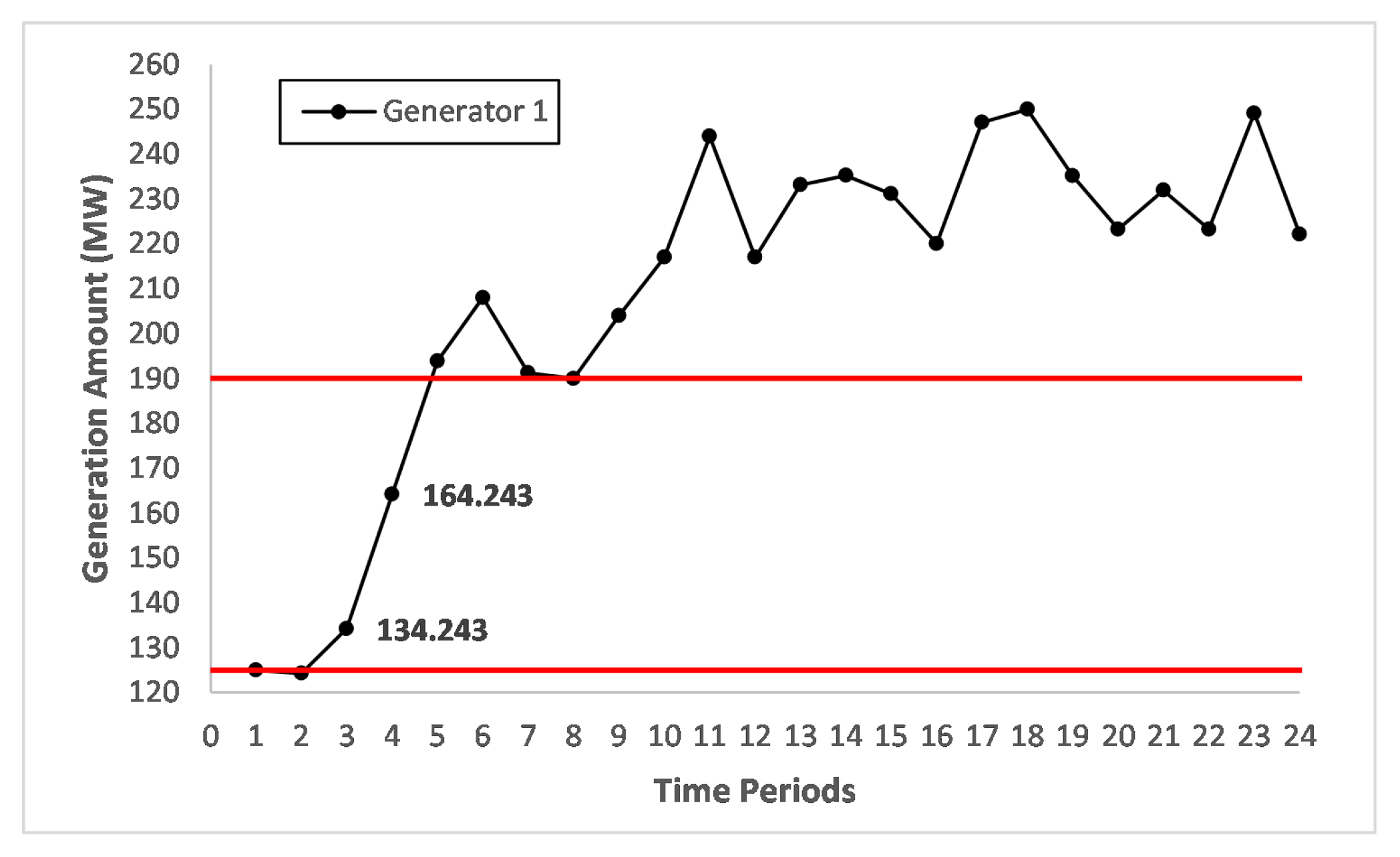
Then, to verify if our proposed model can represent operations of thermal generators accurately, we present the amount of power generation of generator 1 (i.e., $G_1$) over different time intervals in Figure 2. The dynamic ramping rates (MW/min) of this generator are 2.2, 2, and 1.8 for generation ranges (MW) (e.g., forbidden zones and normal zones) of 50–125, 125–190 and 190–250, respectively. Among such ranges, the forbidden zone is the generation range (MW) of 125–190, whose boundaries have been marked in red lines in Figure 2, while the others are normal zones.

In Figure 2, it is obvious that the power generation of generator 1 within the forbidden zone lies in time periods 3 and 4, in which the generator ramps up from 134.243 MW to 164.243 MW with a ramping rate of 2 MW/min, reaching the ramping rate limit in the corresponding forbidden zone. In addition, we can observe that the generator enters the forbidden zone after ramping up in time period 2, and then continues ramping up until it leaves the forbidden zone. Thus, it can be verified that our proposed model can imitate the operations of a real-life system accurately, which leads to more reliable and practical solutions.

4.2. Stochastic Conditions

In this section, we test our data-driven risk-averse two-stage stochastic model with the modified IEEE 118-bus systems, which is available online at http://motor.ece.iit.edu/data. In this system, there are 118 buses, 54 thermal generators, 186 transmission lines, 1 wind farm and 1 pumped-storage unit. And corresponding generator data, fuel data and demands data of each bus in each hour are described. We assume that the renewable power generation from the wind farm contributes to 15% of the total demands. Thus, for simplicity, the renewable power output is considered as the negative system load, so that over time the considered net load can be defined as the difference of the net load and the wind power output. In addition, there are 24 time intervals in total, which means that each time interval is 15 min (i.e., $\delta =15$). We compare our proposed model utilizing the $L_1$ and $L_{\infty }$ norms with the traditional stochastic programming model in the modified IEEE 118-bus system with and without pumped-storage units. We summarize the models as follows:

• Data-driven risk-averse TSP model with the $L_1$ norm (DD-1)
• Data-driven risk-averse TSP model with the $L_{\infty }$ norm (DD-Inf)
• Traditional stochastic programming (TTSP)

4.2.1. Data Setting

To generate the set of historical demand data in each time period, we first generate the demand of each bus in each time interval randomly by using the demand data in the corresponding hour offered in IEEE 118-bus system. Then we use the Monte Carlo sampling method based on these demand data, with which as the mean value and a deviation equalling to 30% of its mean. In addition, we set the number of bins to 5 (i.e., $J=5$). And to allocate samples into 5 bins, k-means algorithm is employed.

4.2.2. Effects on Unit Commitment

This experiment aims to test the effects of the involvements of pumped-storage units on the online/offline statues of thermal generators in the system. In addition, we also test how the historical data impact the UC decisions.

Different from deterministic conditions, under stochastic conditions, risk plays a pivotal role in impacting the final optimal solutions of the proposed model. However, when the pumped-storage unit is included in the system, it can play a vital role in compensating for overproduction or underproduction, which is beneficial for overcoming risk, and consequently the corresponding decisions in UCs may be impacted. In addition, in the traditional TSP problem, the probability of each scenario is certain, which leads to risk-neutral decisions. Conversely, in our data-driven model, decisions against the worst-case distribution are provided, leading to risk-averse decisions. Furthermore, when the number of data samples increases, the risk-averse level of the data-driven model decreases, which will have impacts on the corresponding decisions in the UC. Motivated by this idea, to further investigate such effects, we implement the model with the modified 118-bus system with and without the pumped-storage unit when the number of data samples varies. The UC decisions are shown in

Table 3. Online statuses of generator 52 from the 118-bus system under the $L_1$ and $L_{\infty }$ norms.

# of Samples	With PS						Without PS
	T1	T2	T3	T4	T5	T6	T1	T2	T3	T4	T5	T6
5	1	1	1	1	1	1	1	1	1	1	1	1
50	1	1	1	1	1	1	1	1	1	1	1	1
100	1	1	1	1	1	1	1	1	1	1	1	1
500	1	1	0	0	0	0	1	1	1	1	1	1
1000	1	1	0	0	0	0	1	1	1	1	1	1
2000	0	0	0	0	0	0	1	1	0	0	0	0
5000	0	0	0	0	0	0	1	1	0	0	0	0
Risk-neutral	0	0	0	0	0	0	1	1	0	0	0	0

.

From Table 3, it can be observed that generator 52 in the system with the pumped-storage unit remains online less than the generator in the system without the pumped-storage unit. Specifically, when the number of data samples is 500 or 1000, the generator in the system with the pumped-storage unit remains online for only the first two hours, while the other generator remains online during the whole time horizon. Similarly, when the number of data samples is 2000 and 5000, the generator no longer starts up; meanwhile, the other generator remains online for two hours. The same is true for the performances in the risk-neutral situation, in which the probabilities of the corresponding scenarios are certain, whose values are estimated with 20,000 data samples. The reason is that the pumped-storage unit behaves like a reserve for providing compensation for the uncertain demands to hedge against the risk, therefore benefited from this, operators can start up generators to provide power for loads instead of starting them up to prepare for uncertainties. Accordingly, the online time of the generator can be reduced.

In addition, we can also observe that when more historical data are given, in either the system with the pumped-storage unit or the system without such a unit, the generator will remain online for less time, and when the number of data samples is large enough, the decisions in the online/offline statues will be the same as the ones made in the risk-neutral TSP model. The reason is that as the number of data samples increases, the risk-averse level decreases, and a more accurate probability distribution can be obtained that is closer to the true distribution. Thus, the benefit is that operators can make more precise decisions in determining whether or not it is necessary to keep generators online to prepare for uncertainties in the future.

Consequently, pumped-storage units can contribute to reducing the online time of generators under uncertainties by offering compensations to hedge against risk. In addition, when the number of data samples increases, benefiting from decreased risk-averse level, less time is needed for generators to remain online to hedge against possible uncertainties in the future.

4.2.3. Effects on Conservativeness

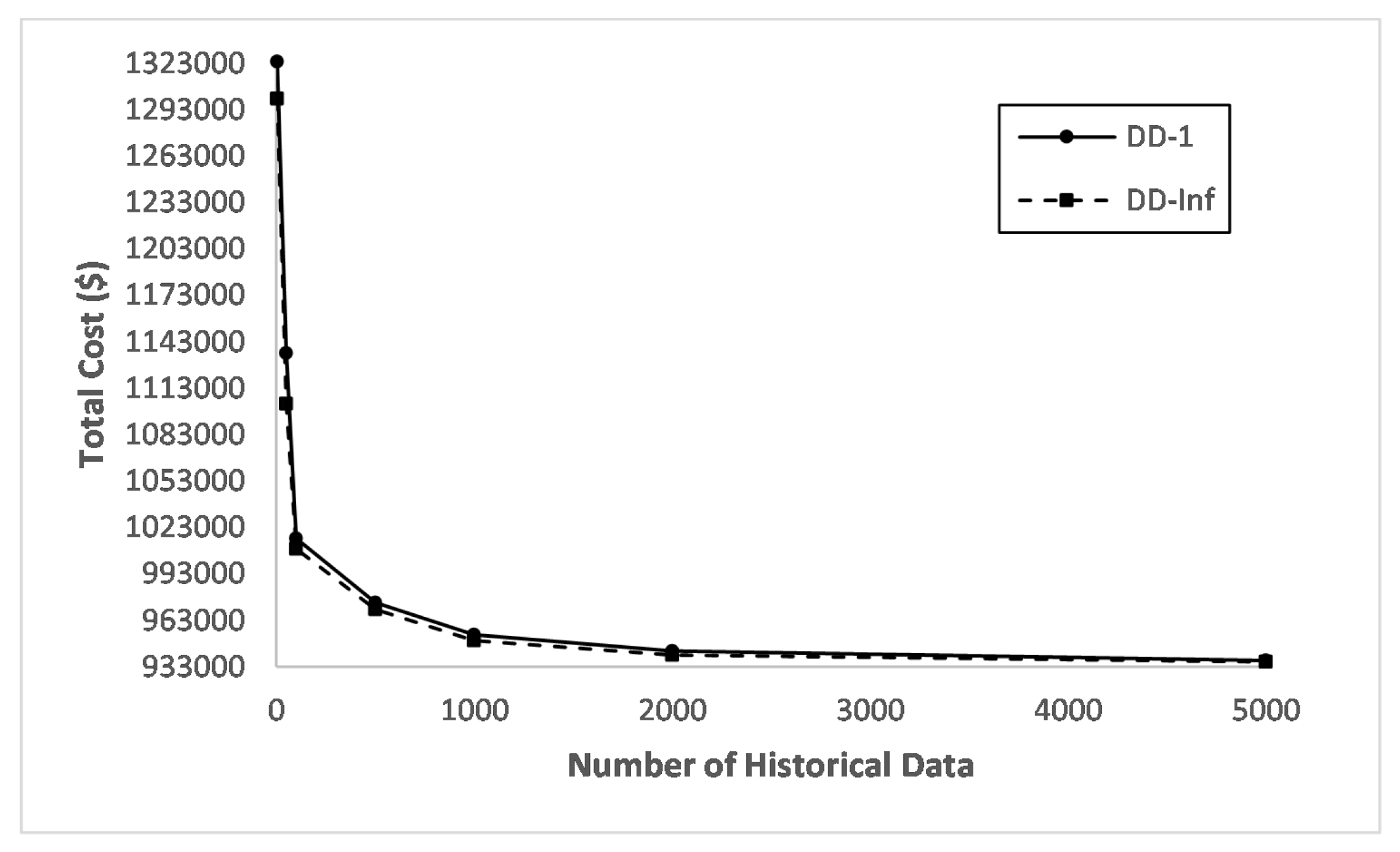
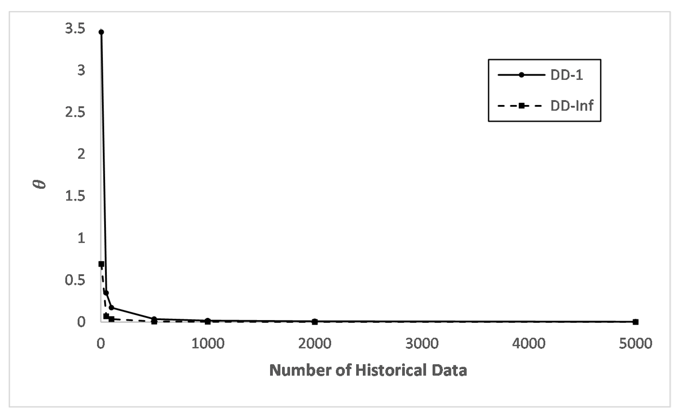
In this section, we study the impacts of historical data on the conservativeness of our proposed model. Specifically, with the fixed confidence level assumed to be 99%, we test our proposed model with the number of data samples increasing from 5 to 5000 in systems with and without the pumped-storage units. The performances are reported in

Table 4. Effects of historical data in the 118-bus system with a pumped-storage unit.

# of Samples	DD-1		DD-Inf		TTSP
	Cost ($)	$\mathit{\theta }$	Cost ($)	$\mathit{\theta }$	Cost ($)
5	1,291,090	3.4539	1,269,230	0.6908	915,730
50	1,108,642	0.3454	1,077,180	0.0691	915,730
100	991,635	0.1727	985,775	0.0345	915,730
500	950,645	0.0345	946,170	0.0069	915,730
1000	934,078	0.0173	930,945	0.0035	915,730
2000	922,343	0.0086	921,354	0.0017	915,730
5000	918,033	0.0035	916,951	0.0007	915,730

and

Table 5. Effects of historical data in the 118-bus system without a pumped-storage unit.

# of Samples	DD-1		DD-Inf		TTSP
	Cost ($)	$\mathit{\theta }$	Cost ($)	$\mathit{\theta }$	Cost ($)
5	1,324,205	3.4539	1,300,183	0.6908	934,718
50	1,135,675	0.3454	1,102,890	0.0691	934,718
100	1,015,812	0.1727	1,009,150	0.0345	934,718
500	974,502	0.0345	970,184	0.0069	934,718
1000	953,610	0.0173	950,047	0.0035	934,718
2000	943,099	0.0086	940,592	0.0017	934,718
5000	937,189	0.0035	936,053	0.0007	934,718

and Figure 3 and Figure 4.

From Table 4 and Table 5 and Figure 3 and Figure 4, we can easily find that in both systems, with an increasing number of data samples, the objective cost decreases, regardless of the norm that is employed. This is because the larger number of data samples leads to a smaller confidence set of the ambiguous distribution, and consequently the results become less conservative. When the number of historical data samples is large enough, the data-driven risk-averse model converges to the risk-neutral model. Furthermore, in Figure 3 and Figure 4, a rapid convergence rate is obviously shown, and when the number of data samples reaches 1000, the objective costs in both two systems almost converge, regardless of the norm that is employed. In further studies of the conservativeness, we find that the objective costs in DD-1 are always higher than those in DD-Inf, which reflects that DD-1 is more conservative than DD-Inf. This is because the $L_1$ norm leads to a larger convergence rate (i.e., $\theta$) than that derived from the $L_{\infty }$ norm, which is shown in Figure 5 (notice here it is reproduced with permission from [6]. IEEE Transactions on Industrial Informatics, 2018.) In practice, operators in the system can choose models based on different norms according to a particular risk-averse level.

Then, we study the value of the extra data in reducing the conservativeness of the model. First, two gaps $Ga{p}_1\left(s\right)$ and $Ga{p}_{\infty }\left(s\right)$ are defined, which mean the objective cost difference between data-driven risk-averse models $DD-1$ and $DD-Inf$ with the traditional two-stage stochastic model (TTSP), respectively. We specify the gaps as follows:

$$\begin{array}{c}\hfill Ga{p}_1\left(s\right)=Cos{t}_1\left(s\right)-Cos{t}_0\left(s\right)\end{array}$$

(61)

$$\begin{array}{c}\hfill Ga{p}_{\infty }\left(s\right)=Cos{t}_{\infty }\left(s\right)-Cos{t}_0\left(s\right)\end{array}$$

(62)

where $Cos{t}_0\left(s\right)$ $Cos{t}_1\left(s\right)$ and $Cos{t}_{\infty }\left(s\right)$ denote the objective costs of the (TTSP), (DD-1) and (DD-Inf), respectively, when the number of data samples equals s.

Based on such definitions, we define the value of the data as

$$\begin{array}{c}\hfill Vo{d}_1(\overline{s},s)=\frac{Ga{p}_1\left(\overline{s}\right)-Ga{p}_1\left(s\right)}{\overline{s}-s},for\overline{s}>s\end{array}$$

(63)

$$\begin{array}{c}\hfill Vo{d}_{\infty }(\overline{s},s)=\frac{Ga{p}_{\infty }\left(\overline{s}\right)-Ga{p}_{\infty }\left(s\right)}{\overline{s}-s},for\overline{s}>s\end{array}$$

(64)

From

Table 6. Value of the extra data in the 118-bus system with a pumped-storage unit.

# of Samples	DD-1		DD-Inf
	${\mathbf{Gap}}_{\mathbf{1}}$	${\mathbf{Vod}}_{\mathbf{1}}$	${\mathbf{Gap}}_{\infty }$	${\mathbf{Vod}}_{\infty }$
5	375,360	N/A	353,500	N/A
50	192,912	4054.40	161,450	4267.77
100	75,905	2340.14	70,045	1828.10
500	34,915	102.47	30,440	99.01
1000	18,348	33.13	15,215	30.45
2000	6613	11.73	5624	9.59
5000	2303	1.43	1221	1.46

and

Table 7. Value of the extra data in the 118-bus system without the pumped-storage unit.

# of Samples	DD-1		DD-Inf
	${\mathbf{Gap}}_{\mathbf{1}}$	${\mathbf{Vod}}_{\mathbf{1}}$	${\mathbf{Gap}}_{\infty }$	${\mathbf{Vod}}_{\infty }$
5	389,487	N/A	365,465	N/A
50	200,957	4189.55	168,172	4384.28
100	81,094	2397.26	74,432	1874.80
500	39,784	103.27	35,466	97.41
1000	18,892	41.78	15,329	40.27
2000	8381	10.51	5874	9.45
5000	2471	1.97	1335	1.51

, we can find the value of the data in the two systems with the two norms employed when the number of data samples varies. It is obvious that as the number of data samples increases, both "Gap" and "Vod" decrease. Additionally, when the number of data samples reaches 5000, both $Vo{d}_1$ and $Vo{d}_{\infty }$ are near 1, which means that the value of the data becomes very limited for our data-driven risk-averse model and that our proposed model can converge to the risk-neutral model rapidly. Therefore, the results demonstrate that we can obtain the relative true solution without too much data being needed.

4.2.4. Effects on Costs

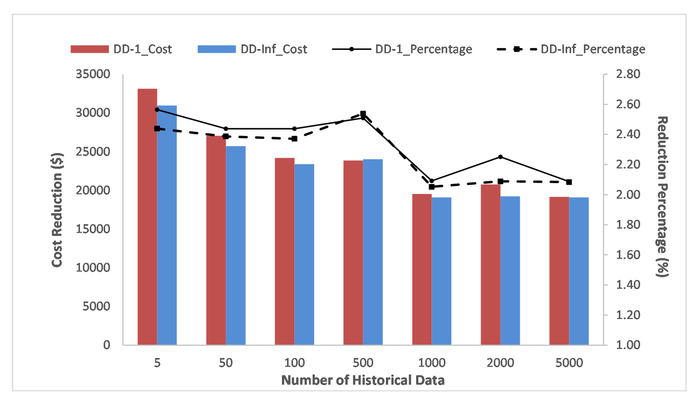
Next, we investigate the impacts of pumped-storage units on objective costs of the system under uncertainties. From Table 4 and Table 5, we can verify that the pumped-storage unit can contribute towards reducing the objective costs in the system under uncertainties. In a further investigation, we determine the decrease in the objective costs when the pumped-storage unit is included and the corresponding percentage equal to the decrease divided by the corresponding optimal cost in the system without the pumped-storage unit. The results are reported in

Table 8. Cost decrease in the 118-bus system.

# of Samples	DD-1 Cost ($)	DD-1 Percentage (%)	DD-Inf Cost ($)	DD-Inf Percentage (%)
5	33,115	2.56	30,953	2.44
50	27,033	2.44	25,710	2.39
100	24,177	2.44	23,375	2.37
500	23,857	2.51	24,014	2.54
1000	19,532	2.09	19,102	2.05
2000	20,756	2.25	19,238	2.09
5000	19,156	2.09	19,102	2.08

and Figure 6.

From Table 8 and Figure 6, we can clearly observe that the objective cost reduction happens when the system includes the pumped-storage unit. Furthermore, as the number of historical data samples increases, regardless of the norm that is employed, both the cost reduction and corresponding cost reduction percentage exhibit decreasing trends. In other words, when the number of data samples is not large, meaning that the risk-averse level is high, the system with a pumped-storage unit can contribute more towards reducing the objective cost. As mentioned previously, the pumped-storage unit plays a pivotal role in hedging against the uncertainty and risk in the system.

5. Conclusions

In this paper, we consider an energy integrated system in which thermal generators, wind farms and pumped-storage units are integrated under uncertainties. We propose a data-driven risk-averse two-stage stochastic model with forbidden zones and dynamic ramping rate limits. We first construct a deterministic model and then extend it to the data-driven risk-averse TSP model. From numerical results, it can be verified that pumped-storage units can contribute towards reducing the objective costs of the system and decreasing the online time of generators. In addition, the results show that in our model, the generator is allowed to enter the forbidden zone, but it has to leave there with the possible highest ramping rate and a fixed ramping direction, which proves that our approach improves the reliability and practicality of the system. Then, we implement our data-driven model to hedge against uncertainties, and from the results obtained by solving the model with Benders decomposition algorithm, we find that pumped-storage units can contribute towards decreasing the online time and the objective costs of the system under uncertainties, especially when the risk-averse level is high. Furthermore, our model utilizes historical data to construct the distributional confidence set, and we demonstrate that when the number of historical data samples is large enough, our proposed model converges to the risk-neutral model.

References

- Daneshi, H. Overview of Renewable Energy Portfolio in CAISO - Operational and Market Challenges. In Proceedings of the 2018 IEEE Power Energy Society General Meeting (PESGM), Portland, OR, USA, 5–9 August 2018; pp. 1–5. [Google Scholar] [CrossRef]
- Guan, Y.; Pan, K.; Zhou, K. Polynomial time algorithms and extended formulations for unit commitment problems. IISE Trans. 2018, 50, 735–751. [Google Scholar] [CrossRef] [Green Version]
- Denholm, P.; O’Connell, M.; Brinkman, G.; Jorgenson, J. Overgeneration from Solar Energy in California. A Field Guide to the Duck Chart; Technical Report; National Renewable Energy Laboratory (NREL): Golden, CO, USA, 2015.
- Brown, P.D.; Lopes, J.P.; Matos, M.A. Optimization of pumped storage capacity in an isolated power system with large renewable penetration. IEEE Trans. Power Syst. 2008, 23, 523–531. [Google Scholar] [CrossRef]
- Zhao, C.; Guan, Y. Data-driven stochastic unit commitment for integrating wind generation. IEEE Trans. Power Syst. 2016, 31, 2587–2596. [Google Scholar] [CrossRef]
- Ziliang, J.; Pan, K.; Fan, L.; Ding, T. Data-Driven Look-Ahead Unit Commitment Considering Forbidden Zones and Dynamic Ramping Rates. IEEE Trans. Ind. Inform. 2018, 15, 3267–3276. [Google Scholar] [CrossRef]
- Lee, F.N.; Breipohl, A.M. Reserve constrained economic dispatch with prohibited operating zones. IEEE Trans. Power Syst. 1993, 8, 246–254. [Google Scholar] [CrossRef]
- Li, T.; Shahidehpour, M. Dynamic ramping in unit commitment. IEEE Trans. Power Syst. 2007, 22, 1379–1381. [Google Scholar] [CrossRef]
- Yang, C.J.; Jackson, R.B. Opportunities and barriers to pumped-hydro energy storage in the United States. Renew. Sustain. Energy Rev. 2011, 15, 839–844. [Google Scholar] [CrossRef]
- Ma, T.; Yang, H.; Lu, L. Feasibility study and economic analysis of pumped hydro storage and battery storage for a renewable energy powered island. Energy Convers. Manag. 2014, 79, 387–397. [Google Scholar] [CrossRef]
- Tuohy, A.; O’Malley, M. Pumped storage in systems with very high wind penetration. Energy Policy 2011, 39, 1965–1974. [Google Scholar] [CrossRef]
- Korpaas, M.; Holen, A.T.; Hildrum, R. Operation and sizing of energy storage for wind power plants in a market system. Int. J. Electr. Power Energy Syst. 2003, 25, 599–606. [Google Scholar] [CrossRef]
- Zhang, N.; Kang, C.; Kirschen, D.S.; Xia, Q.; Xi, W.; Huang, J.; Zhang, Q. Planning pumped storage capacity for wind power integration. IEEE Trans. Sustain. Energy 2013, 4, 393–401. [Google Scholar] [CrossRef]
- Zhao, P.; Wang, J.; Dai, Y. Capacity allocation of a hybrid energy storage system for power system peak shaving at high wind power penetration level. Renew. Energy 2015, 75, 541–549. [Google Scholar] [CrossRef]
- Bussar, C.; Moos, M.; Alvarez, R.; Wolf, P.; Thien, T.; Chen, H.; Cai, Z.; Leuthold, M.; Sauer, D.U.; Moser, A. Optimal allocation and capacity of energy storage systems in a future European power system with 100% renewable energy generation. Energy Procedia 2014, 46, 40–47. [Google Scholar] [CrossRef]
- Zidar, M.; Georgilakis, P.S.; Hatziargyriou, N.D.; Capuder, T.; Škrlec, D. Review of energy storage allocation in power distribution networks: applications, methods and future research. IET Gener. Transm. Distrib. 2016, 10, 645–652. [Google Scholar] [CrossRef]
- Wang, Q.; Guan, Y.; Wang, J. A chance-constrained two-stage stochastic program for unit commitment with uncertain wind power output. IEEE Trans. Power Syst. 2012, 27, 206–215. [Google Scholar] [CrossRef]
- Wang, Q.; Wang, J.; Guan, Y. Stochastic unit commitment with uncertain demand response. IEEE Trans. Power Syst. 2013, 28, 562–563. [Google Scholar] [CrossRef]
- Papavasiliou, A.; He, Y.; Svoboda, A. Self-commitment of combined cycle units under electricity price uncertainty. IEEE Trans. Power Syst. 2015, 30, 1690–1701. [Google Scholar] [CrossRef]
- Niknam, T.; Azizipanah-Abarghooee, R.; Narimani, M.R. An efficient scenario-based stochastic programming framework for multi-objective optimal micro-grid operation. Appl. Energy 2012, 99, 455–470. [Google Scholar] [CrossRef]
- Farzin, H.; Fotuhi-Firuzabad, M.; Moeini-Aghtaie, M. Stochastic energy management of microgrids during unscheduled islanding period. IEEE Trans. Ind. Inform. 2017, 13, 1079–1087. [Google Scholar] [CrossRef]
- Ortega-Vazquez, M.A.; Kirschen, D.S. Estimating the spinning reserve requirements in systems with significant wind power generation penetration. IEEE Trans. Power Syst. 2009, 24, 114–124. [Google Scholar] [CrossRef]
- Pozo, D.; Contreras, J. A chance-constrained unit commitment with an n − K security criterion and significant wind generation. IEEE Trans. Power Syst. 2013, 28, 2842–2851. [Google Scholar] [CrossRef]
- Street, A.; Oliveira, F.; Arroyo, J.M. Contingency-Constrained Unit Commitment With n − K Security Criterion: A Robust Optimization Approach. IEEE Trans. Power Syst. 2011, 26, 1581–1590. [Google Scholar] [CrossRef]
- Jiang, R.; Wang, J.; Guan, Y. Robust Unit Commitment With Wind Power and Pumped Storage Hydro. IEEE Trans. Power Syst. 2012, 27, 800–810. [Google Scholar] [CrossRef]
- Jiang, R.; Zhang, M.; Li, G.; Guan, Y. Two-stage network constrained robust unit commitment problem. Eur. J. Oper. Res. 2014, 234, 751–762. [Google Scholar] [CrossRef]
- Chen, Y.; Wang, Q.; Wang, X.; Guan, Y. Applying robust optimization to MISO look-ahead commitment. In Proceedings of the 2014 IEEE PES General Meeting, Conference & Exposition, National Harbor, MD, USA, 27–31 July 2014; pp. 1–5. [Google Scholar] [CrossRef]
- Wu, W.; Chen, J.; Zhang, B.; Sun, H. A Robust Wind Power Optimization Method for Look-Ahead Power Dispatch. IEEE Trans. Sustain. Energy 2014, 5, 507–515. [Google Scholar] [CrossRef]
- Bertsimas, D.; Sim, M. The price of robustness. Oper. Res. 2004, 52, 35–53. [Google Scholar] [CrossRef]
- Lorca, A.; Sun, X.A. Adaptive robust optimization with dynamic uncertainty sets for multi-period economic dispatch under significant wind. IEEE Trans. Power Syst. 2015, 30, 1702–1713. [Google Scholar] [CrossRef]
- Pan, K.; Guan, Y.; Watson, J.; Wang, J. Strengthened MILP Formulation for Certain Gas Turbine Unit Commitment Problems. IEEE Trans. Power Syst. 2016, 31, 1440–1448. [Google Scholar] [CrossRef]
- Carrion, M.; Arroyo, J.M. A computationally efficient mixed-integer linear formulation for the thermal unit commitment problem. IEEE Trans. Power Syst. 2006, 21, 1371–1378. [Google Scholar] [CrossRef]
- Fan, L.; Pan, K.; Guan, Y. A strengthened mixed-integer linear programming formulation for combined-cycle units. Eur. J. Oper. Res. 2019, 275, 865–881. [Google Scholar] [CrossRef]
- Liu, X. On compact formulation of constraints induced by disjoint prohibited-zones. IEEE Trans. Power Syst. 2010, 25, 2004–2005. [Google Scholar] [CrossRef]
- Ding, T.; Bo, R.; Gu, W.; Sun, H. Big-M based MIQP method for economic dispatch with disjoint prohibited zones. IEEE Trans. Power Syst. 2014, 29, 976–977. [Google Scholar] [CrossRef]
- Correa-Posada, C.M.; Morales-España, G.; Dueñas, P.; Sánchez-Martín, P. Dynamic ramping model including intraperiod ramp-rate changes in unit commitment. IEEE Trans. Sustain. Energy 2017, 8, 43–50. [Google Scholar] [CrossRef]
- CAISO. Generator Forbidden Operating Regions. 2016. Available online: https://www.caiso.com/Documents/2360.pdf (accessed on 18 April 2019).
- Pan, K.; Guan, Y. Data-driven risk-averse stochastic self-scheduling for combined-cycle units. IEEE Trans. Ind. Inform. 2017, 13, 3058–3069. [Google Scholar] [CrossRef]
- Benders, J.F. Partitioning procedures for solving mixed-variables programming problems. Numerische Mathematik 1962, 4, 238–252. [Google Scholar] [CrossRef]
- Van Slyke, R.M.; Wets, R. L-shaped linear programs with applications to optimal control and stochastic programming. SIAM J. Appl. Math. 1969, 17, 638–663. [Google Scholar] [CrossRef]
- De, G.; Tan, Z.; Li, M.; Huang, L.; Song, X. Two-Stage Stochastic Optimization for the Strategic Bidding of a Generation Company Considering Wind Power Uncertainty. Energies 2018, 11, 3527. [Google Scholar] [CrossRef]
Figure 1.
Illustration of the forbidden zones and dynamic ramping rates.
Figure 2.
Dispatch results of generator 1.
Figure 3.
Effects of historical data on the total cost in the 118-bus system with the pumped-storage unit.
Figure 4.
Effects of historical data on the total cost in the 118-bus system without the pumped-storage unit.
Figure 5.
Effects of historical data on .
Figure 6.
Effects of historical data on the decrease in the total cost in the 118-bus system.