Accurate Assessment of Decoupled OLTC Transformers to Optimize the Operation of Low-Voltage Networks

Abstract

Voltage control in active distribution networks must adapt to the unbalanced nature of most of these systems, and this requirement becomes even more apparent at low voltage levels. The use of transformers with on-load tap changers is gaining popularity, and those that allow different tap positions for each of the three phases of the transformer are the most promising. This work tackles the exact approach to the voltage optimization problem of active low-voltage networks when transformers with on-load tap changers are available. A very rigorous approach to the electrical model of all the involved components is used, and common approaches proposed in the literature are avoided. The main aim of the paper is twofold: to demonstrate the importance of being very rigorous in the electrical modeling of all the components to operate in a secure and effective way and to show the greater effectiveness of the decoupled on-load tap changer over the usual on-load tap changer in the voltage regulation problem. A low-voltage benchmark network under different load and distributed generation scenarios is tested with the proposed exact optimal solution to demonstrate its feasibility.

1. Introduction

Low-voltage (LV) networks are generating increasing interest for a variety of reasons, such as the massive deployment of smart meters [1], the growing presence of distributed renewable generation (DG) [2], and important new components such as electric vehicles (EVs) and storage devices (SDs) [3]. The eruption of all these new actors has completely changed the approach to planning and operating voltage levels in light of two main facts. Firstly, new low-carbon technologies cause new planning and operational problems that were never taken into account when passive consumers were the only clients connected to this voltage level [4,5,6]. Secondly, a much greater extent of new and detailed information is available from smart meters [7], generating a very valuable starting point for tackling these new planning and operational challenges.

Power quality is one of the main concerns in an LV grid. Classical consumers and the aforementioned new participants demand quality from the distribution utility, with the level of voltage being one of the most important aspects. Many distribution companies have reported voltage complaints because of steady-state undervoltages and/or overvoltages [8,9,10,11,12].

On the one hand, permanent undervoltages/overvoltages are one of the issues that consumers are more concerned about. Both phenomena can lead to issues such as shutdowns, malfunctions, overheating, premature failures, and poor efficiency of consumer devices [13]. On the other hand, the level of supplied voltage is also of great relevance to the distribution company, and not only because of consumer complaints. It is well known that voltage control allows utilities to improve the operation efficiency of their networks by minimizing power losses [14], taking advantage of conservation voltage reduction [15], delaying new investments [16], and so on.

Some of the most common causes of undervoltage and overvoltage are the unsuitable tap setting of secondary distribution transformers, improper voltage regulation setting of substations, transformer/cable overloads (for undervoltages), and three-phase imbalances. As a general rule, the voltage of monitored networks tends to be closer to the upper voltage limits than the lower ones [11,12], which implies that the irruption of massive embedded generation can even worsen the frequency and duration of overvoltage phenomena [17].

The above details highlight that voltage control in low-voltage grids is of great relevance. Volt/var control of distribution networks has usually been confined to the medium-voltage (MV) level by using the on-load tap changer (OLTC) of high-voltage (HV)/MV transformers located at substations, capacitor banks, and/or step voltage regulators that are allocated along distribution feeders. Advanced volt/var control solutions specifically adapted to active distribution systems propose the use of new control sources: utility and customer-owned distributed power electronics (mainly those linked to DG), energy storage systems, power curtailment of DG generation and/or load, etc. All these novel control tools are well developed in the literature but not so much in practice [18,19]. For LV levels, in practice, most utilities with a European-style network design use only the secondary distribution transformers equipped with off-load tap changers to control voltages. Once again, the use of both the traditional and novel MV volt/var control solutions mentioned above has been intensively proposed in the most current literature, but it is not applied in practice [20,21,22,23,24,25,26,27,28,29,30,31]. The use of OLTC transformers in secondary distribution substations is currently the closest to realizing an LV reality [19,32,33,34,35]. This paper focuses on this last point: the use of OLTC MV/LV transformers (OLTCST) to control voltage in LV networks.

Depending on the technology, two different methods of operating an OLTCST are possible: (1) a synchronized tap change among the three phases or (2) decoupled control [32]. Most previous works have dealt with uniform and common tap positions for all three phases of the MV/LV-controlled transformer (3P-OLTCST) [19,20,21,28,30,31,33,34,35], but increasingly, more tap position settings among transformer phases are being proposed (1P-OLTCST) [24,25,29,32,36]. Decoupled control is obviously a great deal more attractive for LV networks because of their unbalanced nature.

Regardless of whether uniform or non-uniform phase tap movements are employed, there are two main methodologies for fulfilling voltage control: rule-based approaches or analytical solutions. Among the first group, different levels of “intelligence” have been proposed to reach a global solution that is as close as possible to the optimal one [21,24,28,32]. Analytical approaches are integrated solutions that solve an optimization problem to determine the best control actions that both minimize an objective function and fulfill all the electrical constraints [29,30,36]. While rule-based solutions reach a suboptimal solution but are easier to implement and need less network information, analytical approaches are more rigorous from a mathematical point of view and ensure not only an optimal solution but also that all the variables are within their limits. Until recently, the main drawbacks of applying analytical solutions laid in their computational cost (both programming and time consumed) and the necessity of having detailed models of the controlled network and scenarios of demand/generation for each time. Nowadays, the current trend toward active LV networks implies not only that these barriers are starting to disappear but also that the current knowledge of networks and power demand/dispersed generation can generate great value for distribution utilities [37].

On this basis, this paper tackles the optimal voltage control problem of European LV networks by using decoupled OLTC transformers (1P-OLTCST) and implementing an analytical solution. Previous works proposing analytical approaches to this problem have been mostly confined to American MV networks [30,36].

The authors in [30] use as voltage controllers 3P-OLTCST and PV inverters to minimize power losses, voltage violations, and lines loading; a three-phase simplified line model is assumed for four-wire three-phase lines as well as approximated voltage drop equations; no electrical model is taken into account for 3P-OLTCTS. The optimization problem proposed in [36] works with 1P-OLTCTS and static voltage converters, and although three-phase transformer models are incorporated into the mathematical problem, once again a three-phase simplified line model is considered. In addition, ground resistances different from zero are not taken into consideration. An optimal solution specifically designed for European MV and LV grids (both integrated) is published in [29]. In that approach, the optimal location and size of dSTATCOM, SD, and 3P-OLTCST, as well as the reactive contribution by DG’s inverters are determined in order to manage voltage and minimize investment, operation, and maintenance costs. However, no details are provided in [29] to clearly deduce if detailed models for transformers, lines, and ground resistances are considered. In contrast, this new proposed work takes note of previous shortcomings and considers them warnings of the importance of neutral grounding considerations [38] and the need to use a rigorous model for all system components [39]. Therefore, the main novelties of this paper are the following:

• The optimization problem associated with the optimal voltage control of unbalanced LV networks by using transformers with OLTCs as control devices is rigorously defined and solved. No approximations are assumed and detailed models for all the components are considered:

  -

  three-phase model of three-phase transformers, incorporating also their ground connection design;

  -

  three-phase four-wire lines are neither reduced to a three-phase model nor decoupled,

  -

  any earthing system type is taken into account.

• The former optimization problem is implemented and solved, comparing the real possibilities of 1P-OLTCST versus 3P-OLTCST.

From the knowledge of the authors, no previous work has posed this voltage optimization problem for unbalanced LV networks with such a level of detail, so the results are quite conclusive.

The layout of the paper is as follows: Section 2 describes the framework in which voltage control is performed, and Section 3 tackles the mathematical problem definition by considering the appropriate model for each of the components entering the studied system. Section 4 shows the obtained results for a European low-voltage benchmark system to demonstrate both the benefits resulting from decoupled tap control compared with the traditional uniform three-phase tap control and the importance of the model to carry out effective control. Finally, Section 5 presents the most relevant conclusions and suggests the next steps for future work.

2. Low-Voltage European Networks

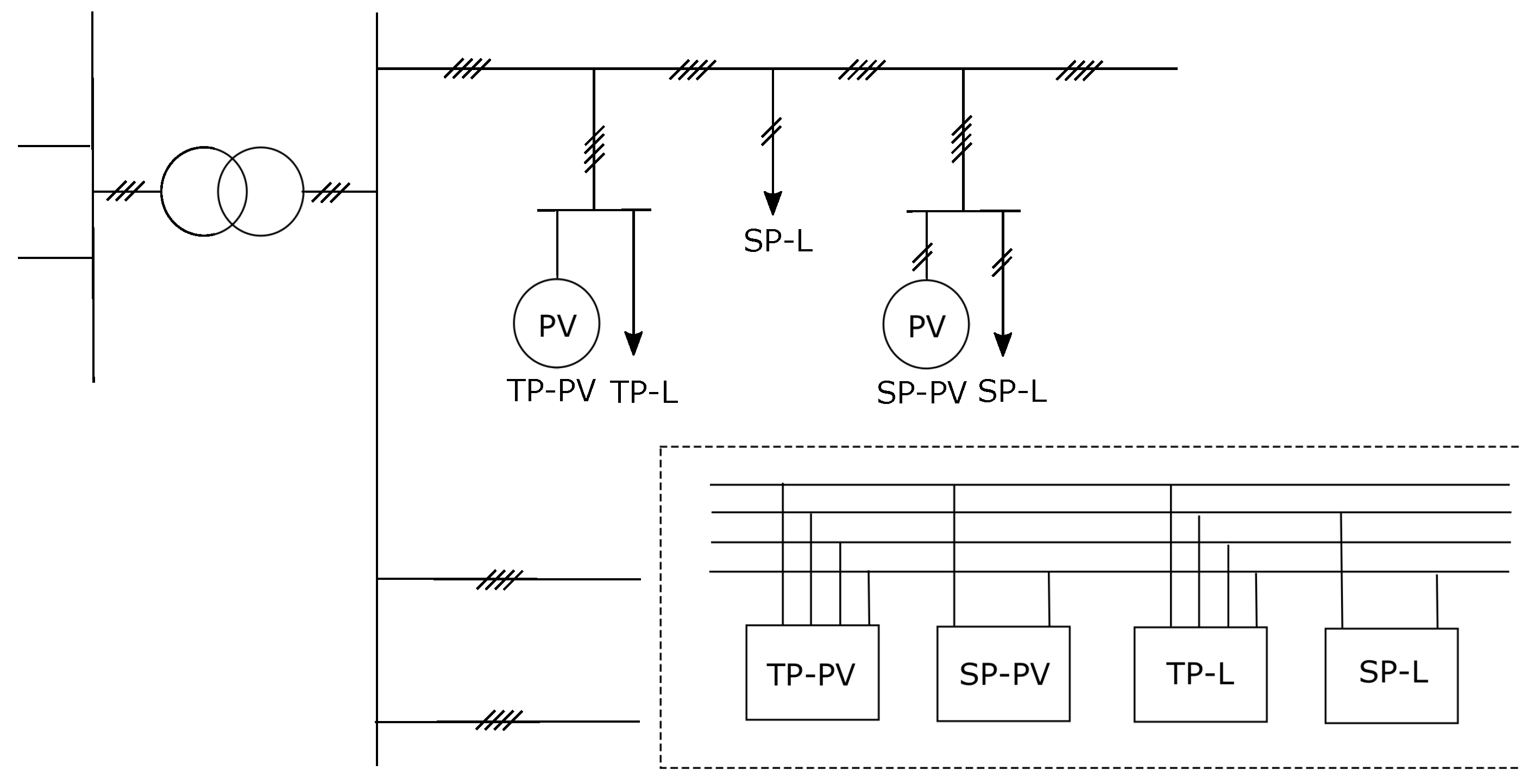
Distribution networks with the so-called European design are not limited to Europe; in fact, they are widely used all over the world. Many other countries adopted this arrangement, and the European design is well established, even in urban North American distribution networks [40]. The general structure of European distribution systems consists of a three-phase medium-voltage system in which three phase distribution transformers are connected to feed a large number of consumers/distributed generators connected to the three-phase low-voltage grid. An LV network can have a radial, ring, or meshed structure, but most are operated radially. Figure 1 depicts the schema of a typical radial European low-voltage grid.

Distribution or secondary transformers are large three-phase transformers (normally between 100 and 1000 kVA), with 20 kV/400 V being the most typical normalized voltages. One of the most common configurations is delta-wye because this arrangement prevents imbalance on the low-voltage side (due to unbalanced consumption) by transferring loads to the MV level. Nowadays, most of these secondary transformers have off-load tap changers, and OLTC transformers are considered in the rest of the paper, as justified in Section 1.

Low-voltage lines are three-phase four-wire lines that are usually underground cables in urban areas and overhead lines in rural ones. LV networks are primarily earthed at the star-point of the MV/LV transformer. The earthing at the customer location is usually by the public supply network, and it is most often performed by earthing the neutral along different points of the low-voltage feeder.

Single-phase and three-phase consumers connect to the low-voltage network, with the former more prevalent than the latter. With distributed generators, mainly those that are photovoltaic, single-phase or three-phase consumers can also be connected, depending on the nominal power [41]. Single-phase clients connect one phase to the neutral conductor in an attempt to distribute them among the three phases so that the total three-phase equivalent net load from the secondary side of the transformer is as balanced as possible. In practice, although the same kind of single-phase consumers are equally distributed among all three phases, imbalances occur as a consequence of the different hourly load patterns. These imbalances are one of the main concerns of utility engineers.

One of the main conclusions resulting from the former design is that a three-phase model that takes into account all phases and the neutral must be considered, and a single-phase equivalent circuit is not valid for analyzing the whole power system. Even a decoupled single-phase circuit to study each of the three phases independently would lead to erroneous results [42].

3. Optimization Problem

The radial LV system under study comprises $N+1$ nodes (buses are numbered from 0). Without loss of generality, bus 0 applies to the MV side of the distribution transformer at the head of the whole LV grid. The set of three-phase buses, loads, and generators are denoted by B, L, and G, respectively. Note that the number of branches is equal to the number of buses minus one because of the radiality of the system.

The optimization problem to be solved involves determining the best value of the tap positions of each phase of a three-phase distribution transformer in order to optimize the operation of the whole system at a specific time $\mathit{h}$ while keeping all quantities within limits. These tap positions are the control variables of the problem. The dependent variables are phase–ground voltages at each node i, ${\mathcal{U}}_i^T={\left[{\mathcal{U}}_{iq}\right]}^T={\left[{\mathcal{U}}_{ia}{\mathcal{U}}_{ib}{\mathcal{U}}_{ib}{\mathcal{U}}_{in}\right]}^T$, phase current injections at each node i, ${\mathcal{I}}_i^T={\left[{\mathcal{I}}_{iq}\right]}^T={\left[{\mathcal{I}}_{ia}{\mathcal{I}}_{ib}{\mathcal{I}}_{ib}{\mathcal{I}}_{in}\right]}^T$, phase current flows through series branch $ij$, ${\mathcal{I}}_{ij}^T={\left[{\mathcal{I}}_{ij,q}\right]}^T={\left[{\mathcal{I}}_{ij,a}{\mathcal{I}}_{ij,b}{\mathcal{I}}_{ij,c}{\mathcal{I}}_{ij,n}\right]}^T$, and current ${\mathcal{I}}_{ig}$ through the ground resistor at bus i ($i,j,k$ are indexes associated with buses; $\left(ij\right)$ denotes a series branch between buses i and j; p refers to each of the three phases $a,b,c$; the neutral phase is denoted by n; and the indexes $m,q$ denote any of the three phases as well as the neutral).

The next subsections detail the objective function and constraints associated with the optimization problem to be solved. Equality and inequality constraints result from modeling the electrical behavior of all the components and from considering all of the operational limits imposed by these components and the fulfillment of required standards. The phase domain and phase coordinates are considered to set out the problem, with computations being performed in physical units. In what follows, each complex equation that appears should be transformed into two equivalent real equations; this step is omitted throughout the paper.

3.1. Objective Function

The minimization of power losses is proposed as the main target objective. The power losses of the system can be formulated from a power balance point of view, so the following objective Function (1) results:

$$min\Re \left({\mathcal{S}}_{loss}\right)=min\Re \left({\mathcal{U}}_0^T{\mathcal{I}}_0^{*}\right)+\sum _{i=1}^{N+1}\sum _p\left[{\mathcal{S}}_{ip}^G+{\mathcal{S}}_{ip}^L\right],$$

(1)

where ${\mathcal{S}}_{ip}^G$ refers to the generated specified power at phase p of node i, and ${\mathcal{S}}_{ip}^L$ denotes the demanded complex power of a load at phase p of node i. Note the net injected power by shunt elements connected to bus i is ${\mathcal{S}}_{ip}={\mathcal{S}}_{ip}^G+{\mathcal{S}}_{ip}^L$, so the generated power ${\mathcal{S}}_{ip}^G$ takes values greater than zero while the demanded load ${\mathcal{S}}_{ip}^L$ takes negative values. It is important to underline that the objective Function (1) considers all losses, namely power losses in the transformer, lines, and ground resistors.

The minimization of imbalances, voltage drops, or neutral currents are other common objective functions to consider. Power losses have commonly been chosen since they represent a well-defined single key index whose lowest value is usually linked to the best voltage profile. Other possible choices are those defined at a node or branch level, and such options necessitate the definition of a single index for any of them (for example, if the minimization of voltage drops was chosen, a possible voltage index to quantify this objective could be the addition of the deviation of each node voltage from its nominal value). In sum, an objective function that differs from the minimization of power losses could be set out.

3.2. Medium-Voltage Grid Equivalent

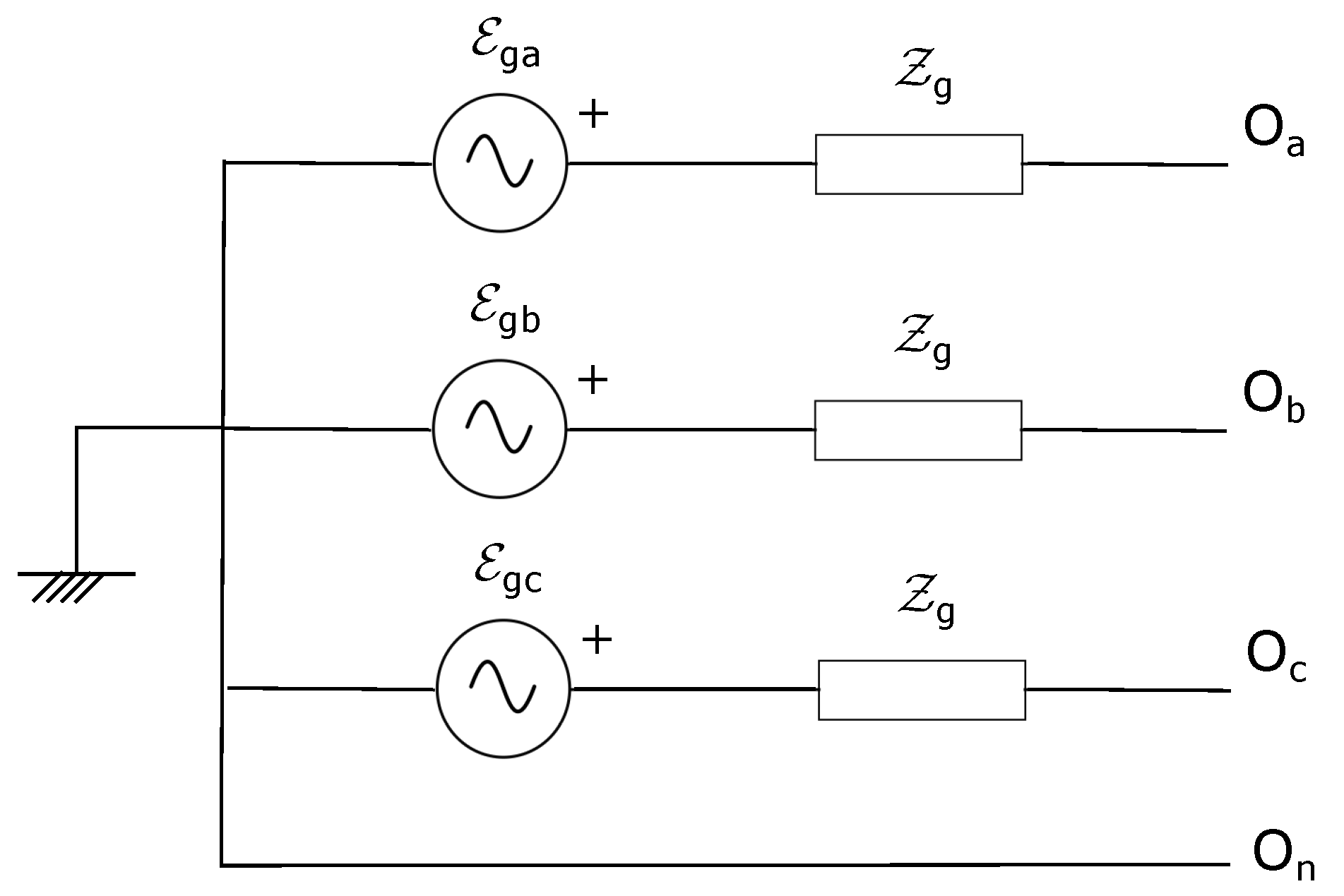
A three-phase Thévenin equivalent network is considered in the model of an MV grid that is upstream of the distribution transformer, as depicted in Figure 2. A rigid grounded wye three-phase balanced ideal voltage source ${\mathcal{E}}_g^T={\left[E_g\underline{|\phantom{(}0}{E}_g\underline{|\phantom{(}-120}{E}_g\underline{|\phantom{(}120}0\right]}^T$ in series with a single impedance ${\mathcal{Z}}_g$ is assumed. These MV equivalent network parameters correspond with the actual operational medium voltage and the short-circuit impedance, respectively.

3.3. Distribution Transformer Model

A complete and exact model for a three-phase transformer requires of a large number of short-circuit experiments, some of which are difficult to implement, depending on the type of transformer (common-core or shell-type integrated three-phase devices) [43]. A well-accepted starting assumption is that the three-phase transformer consists of three independent and identical single-phase transformers [43,44] since it has been demonstrated that the resulting inaccuracies from this simplification are subtle [43,45]. In this context, modeling the three-phase transformer starts by considering a single-phase transformer such as that shown in Figure 3, whose admittance-bus-based electrical model follows Equation (2):

$$\left[\begin{array}{c}{\mathcal{I}}_1\\ {\mathcal{I}}_2\end{array}\right]=\left[\begin{array}{cc}{\mathcal{Y}}_t+{\mathcal{Y}}_m& -r{\mathcal{Y}}_t\\ -r{\mathcal{Y}}_t& r^2{\mathcal{Y}}_t\end{array}\right]\left[\begin{array}{c}{\mathcal{U}}_1\\ {\mathcal{U}}_2\end{array}\right],$$

(2)

where ${\mathcal{Y}}_t$ is the short-circuit or leakage admittance, ${\mathcal{Y}}_m$ is the open-circuit or magnetizing admittance—with both referring to the primary side of the transformer—and r is the transformer ratio.

The electrical model associated with three independent and decoupled single-phase transformers follows Equation (3), in which the three single-phase transformers are denoted by a, b, c, and their primary and secondary sides are numbered consecutively from 1 to 6. For further developments, three different transformer ratios are adopted for each of the individual phases and are denoted by $r_a$, $r_b$, and $r_c$.

$$\left[\begin{array}{c}{\mathcal{I}}_1\\ {\mathcal{I}}_2\\ {\mathcal{I}}_3\\ {\mathcal{I}}_4\\ {\mathcal{I}}_5\\ {\mathcal{I}}_6\end{array}\right]=\left[\begin{array}{cccccc}{\mathcal{Y}}_{ta}+{\mathcal{Y}}_{ma}& -r_a{\mathcal{Y}}_{ta}& 0& 0& 0& 0\\ -r_a{\mathcal{Y}}_{ta}& r_a^2{\mathcal{Y}}_{ta}& 0& 0& 0& 0\\ 0& 0& {\mathcal{Y}}_{tb}+{\mathcal{Y}}_{mb}& -r_b{\mathcal{Y}}_{tb}& 0& 0\\ 0& 0& -r_b{\mathcal{Y}}_{tb}& r_b^2{\mathcal{Y}}_{tb}& 0& 0\\ 0& 0& 0& 0& {\mathcal{Y}}_{tc}+{\mathcal{Y}}_{mc}& -r_c{\mathcal{Y}}_{tc}\\ 0& 0& 0& 0& -r_c{\mathcal{Y}}_{tc}& r_c^2{\mathcal{Y}}_{tc}\end{array}\right]\left[\begin{array}{c}{\mathcal{U}}_1\\ {\mathcal{U}}_2\\ {\mathcal{U}}_3\\ {\mathcal{U}}_4\\ {\mathcal{U}}_5\\ {\mathcal{U}}_6\end{array}\right]$$

(3)

Different three-phase transformers can result from these three independent single-phase transformers, depending on the connections between their terminal pairs, with wye and delta connections the most commonly used. The specific connection for the three-phase transformer allows for the formulation of mathematical expressions that link the voltages and currents of the three single-phase transformers with the voltages and currents of the high- and low-voltage sides of the three-phase transformer. For example, Figure 4 shows the $\Delta -$yg configuration, one of the most common schemes in European low-voltage networks. For this configuration, the relations among the former electrical quantities are defined by Equations (4) and (5), as can be easily deduced from Figure 4.

$$\left[\begin{array}{c}{\mathcal{U}}_1\\ {\mathcal{U}}_2\\ {\mathcal{U}}_3\\ {\mathcal{U}}_4\\ {\mathcal{U}}_5\\ {\mathcal{U}}_6\end{array}\right]=\left[\begin{array}{ccccccc}1& -1& 0& 0& 0& 0& 0\\ 0& 0& 0& 1& 0& 0& -1\\ 0& 1& -1& 0& 0& 0& 0\\ 0& 0& 0& 0& 1& 0& -1\\ -1& 0& 1& 0& 0& 0& 0\\ 0& 0& 0& 0& 0& 1& -1\end{array}\right]\left[\begin{array}{c}{\mathcal{U}}_A\\ {\mathcal{U}}_B\\ {\mathcal{U}}_C\\ {\mathcal{U}}_a\\ {\mathcal{U}}_b\\ {\mathcal{U}}_c\\ {\mathcal{U}}_n\end{array}\right]=N\left[\begin{array}{c}{\mathcal{U}}_A\\ {\mathcal{U}}_B\\ {\mathcal{U}}_C\\ {\mathcal{U}}_a\\ {\mathcal{U}}_b\\ {\mathcal{U}}_c\\ {\mathcal{U}}_n\end{array}\right]$$

(4)

$$\left[\begin{array}{c}{\mathcal{I}}_A\\ {\mathcal{I}}_B\\ {\mathcal{I}}_C\\ {\mathcal{I}}_a\\ {\mathcal{I}}_b\\ {\mathcal{I}}_c\\ {\mathcal{I}}_n\end{array}\right]=N^T\left[\begin{array}{c}{\mathcal{I}}_1\\ {\mathcal{I}}_2\\ {\mathcal{I}}_3\\ {\mathcal{I}}_4\\ {\mathcal{I}}_5\\ {\mathcal{I}}_6\end{array}\right]+\left[\begin{array}{c}0\\ 0\\ 0\\ 0\\ 0\\ \frac{{\mathcal{U}}_n}{R_g}\end{array}\right]$$

(5)

By substituting (3) into (5) and using (4), the final model (6) results for a three-phase $\Delta -$yg transformer that consists of three single-phase transformers (${\mathcal{Y}}_{ta}={\mathcal{Y}}_{tb}={\mathcal{Y}}_{tc}={\mathcal{Y}}_t$, ${\mathcal{Y}}_{ma}={\mathcal{Y}}_{mb}={\mathcal{Y}}_{mc}={\mathcal{Y}}_m$) that are identical in all respects except for their transformer ratios:

$$\left[\begin{array}{c}{\mathcal{I}}_A\\ {\mathcal{I}}_B\\ {\mathcal{I}}_C\\ {\mathcal{I}}_a\\ {\mathcal{I}}_b\\ {\mathcal{I}}_c\\ {\mathcal{I}}_n\end{array}\right]=\left[\begin{array}{ccccccc}2{\mathcal{Y}}_t+2{\mathcal{Y}}_m& -{\mathcal{Y}}_t-{\mathcal{Y}}_m& -{\mathcal{Y}}_t-{\mathcal{Y}}_m& -r_a{\mathcal{Y}}_t& 0& r_c{\mathcal{Y}}_t& (r_a-r_c){\mathcal{Y}}_t\\ -{\mathcal{Y}}_t-{\mathcal{Y}}_m& 2{\mathcal{Y}}_t+2{\mathcal{Y}}_m& -{\mathcal{Y}}_t-{\mathcal{Y}}_m& r_a{\mathcal{Y}}_t& -r_b{\mathcal{Y}}_t& 0& (r_b-r_a){\mathcal{Y}}_t\\ -{\mathcal{Y}}_t-{\mathcal{Y}}_m& -{\mathcal{Y}}_t-{\mathcal{Y}}_m& 2{\mathcal{Y}}_t+2{\mathcal{Y}}_m& 0& r_b{\mathcal{Y}}_t& -r_c{\mathcal{Y}}_t& (r_c-r_b){\mathcal{Y}}_t\\ -r_a{\mathcal{Y}}_t& r_a{\mathcal{Y}}_t& 0& r_a^2{\mathcal{Y}}_t& 0& 0& -r_a^2{\mathcal{Y}}_t\\ 0& -r_b{\mathcal{Y}}_t& r_b{\mathcal{Y}}_t& 0& r_b^2{\mathcal{Y}}_t& 0& -r_b^2{\mathcal{Y}}_t\\ r_c{\mathcal{Y}}_t& 0& -r_c{\mathcal{Y}}_t& 0& 0& r_c^2{\mathcal{Y}}_t& -r_c^2{\mathcal{Y}}_t\\ (r_a-r_c){\mathcal{Y}}_t& (r_b-r_a){\mathcal{Y}}_t& (r_c-r_b){\mathcal{Y}}_t& -r_a^2{\mathcal{Y}}_t& -r_b^2{\mathcal{Y}}_t& -r_c^2{\mathcal{Y}}_t& \begin{array}{c}(r_a^2+r_b^2+r_c^2){\mathcal{Y}}_t\\ +\frac{1}{R_g}\end{array}\end{array}\right]\left[\begin{array}{c}{\mathcal{U}}_A\\ {\mathcal{U}}_B\\ {\mathcal{U}}_C\\ {\mathcal{U}}_a\\ {\mathcal{U}}_b\\ {\mathcal{U}}_c\\ {\mathcal{U}}_n\end{array}\right]$$

(6)

The described procedure allows the final bus admittance matrix to be obtained for any other group connection of the three transformers. Note that to obtain a perfect earth connection of the neutral, i.e., $R_g=0$, the last diagonal element of the three-phase bus admittance matrix is not defined; in this case, ${\mathcal{U}}_n$ is zero and the last row of (6) is omitted. The neutral current flowing through the wye side of the transformer would be obtained by applying Kirchhoff’s current law to the secondary bus of the transformer, as described in Section 3.6.

3.4. Low-Voltage Lines and Ground Resistances

Three-phase four-wire lines are the most common configuration for European low-voltage networks, and short single-phase sections are used to connect single-phase clients to the main three-phase four-wire LV line. The modeling of overhead and underground line segments must be as precise as possible since this model plays an important role in the final solution, as illustrated later. This high accuracy demands for a complete and reliable database in relation to low-voltage lines: the type and size of every conductor, the physical geometry of both overhead and underground lines, the resistance of the earth, etc. This information allows Carsons’s equations [46] to be applied in order to obtain the resistance and the self- and mutual inductive reactance of the conductors that make up the line. These series impedances are shown in Figure 5. A 4 × 4 series impedance matrix ${\mathcal{Z}}_{ij}$ results from this model (7). The series impedance matrix is completely full for a three-phase four-wire line, with only non-null elements in one phase and neutral positions for two-phase or single-phase lines.

$${\mathcal{U}}_i={\mathcal{Z}}_{ij}{\mathcal{I}}_{ij}+{\mathcal{U}}_j=\left[\begin{array}{c}{\mathcal{U}}_{ia}\\ {\mathcal{U}}_{ib}\\ {\mathcal{U}}_{ic}\\ {\mathcal{U}}_{in}\end{array}\right]=\left[\begin{array}{cccc}{\mathcal{Z}}_{ij}^{aa}& {\mathcal{Z}}_{ij}^{ab}& {\mathcal{Z}}_{ij}^{ac}& {\mathcal{Z}}_{ij}^{an}\\ {\mathcal{Z}}_{ij}^{ab}& {\mathcal{Z}}_{ij}^{bb}& {\mathcal{Z}}_{ij}^{bc}& {\mathcal{Z}}_{ij}^{bn}\\ {\mathcal{Z}}_{ij}^{ac}& {\mathcal{Z}}_{ij}^{bc}& {\mathcal{Z}}_{ij}^{cc}& {\mathcal{Z}}_{ij}^{cn}\\ {\mathcal{Z}}_{ij}^{an}& {\mathcal{Z}}_{ij}^{bn}& {\mathcal{Z}}_{ij}^{cn}& {\mathcal{Z}}_{ij}^{nn}\end{array}\right]\left[\begin{array}{c}{\mathcal{I}}_{ij,a}\\ {\mathcal{I}}_{ij,b}\\ {\mathcal{I}}_{ij,c}\\ {\mathcal{I}}_{ij,n}\end{array}\right]+\left[\begin{array}{c}{\mathcal{U}}_{ja}\\ {\mathcal{U}}_{jb}\\ {\mathcal{U}}_{jc}\\ {\mathcal{U}}_{jn}\end{array}\right]$$

(7)

It is common practice to neglect capacitances in the case of low-voltage lines because the lengths of the lines are short. So, throughout this paper, this shunt effect is not considered.

It is not always possible to apply Carson’s equations because the requisite information is not usually available in utility-based data (distance between conductors, height of conductors, earth resistivity, etc.). Instead, positive sequence impedance ${\mathcal{Z}}_1$ and, more rarely, zero sequence impedance ${\mathcal{Z}}_0$ are the only practicable line data. In this last case, the best-approximated series impedance ${\mathcal{Z}}_{ij}^{Aprox}$ is

$${\mathcal{Z}}_{ij}^{Aprox}=\left[\begin{array}{cccc}{\mathcal{Z}}_1& 0& 0& 0\\ 0& {\mathcal{Z}}_1& 0& 0\\ 0& 0& {\mathcal{Z}}_1& 0\\ 0& 0& 0& \frac{{\mathcal{Z}}_0-{\mathcal{Z}}_1}{3}\end{array}\right].$$

(8)

This simplified model is obtained by assuming an identical type of conductor for all phases and the neutral and equal sections, symmetrical spacing between phases (including the neutral), and perfect earthing at both extremes of each line segment [46].

Neutral conductors are commonly grounded at multiple points along the network (neutral grounding) for safety reasons. The values of these resistors depend on the type of earth conductor and electrode, as well as the resistivity of the terrain. These characteristics determine the value of the resistor $R_{ig}$ to consider at each bus i, and the value can ideally move between zero and infinity. If this resistor is a finite value, Ohm’s law is applied (9):

$${\mathcal{U}}_{in}=R_{ig}{\mathcal{I}}_{ig}\forall \mathrm{bus}i\mathrm{earthed}\mathrm{with}\mathrm{a}\mathrm{finite}\mathrm{resistor},$$

(9)

where ${\mathcal{I}}_{ig}$ denotes the current flowing through the ground resistor. Note that ${\mathcal{U}}_{in}$ has a null result for rigid earthing.

If the neutral of bus i is not connected to the ground, that is, $R_{ig}=\infty$, the ground current is forced to be zero (10):

$${\mathcal{I}}_{ig}=0\forall \mathrm{bus}i\mathrm{unearthed}$$

(10)

3.5. Loads and Renewable Generators

Hereinafter, the appropriate model for consumers and renewable generators connected to the low-voltage system is discussed. The optimal power flow analysis discussed throughout this paper deals with the steady state, so static models are considered.

Static load models can be classified into the following groups: exponential, polynomial, linear, comprehensive, static induction motor, and power electronic-interfaced models [47]. Among all these static load models, the constant real and reactive power load model is the most widely used for utilities [47], as a particular case of the polynomial or ZIP model (constant impedance Z, constant current I, and constant power P model). Any other model could be considered if the appropriate parameters for each load are known. For renewable generation, with a focus on PV technologies, a steady-state power injection model is also adopted. PV generators operate by injecting the maximum available power, which varies depending on the irradiance. Similarly, the reactive power injection can be set depending on the standing grid code. Unity power factor operation is a common practice for PV generators connected to LV networks.

Three-phase loads and generators can be connected in wye or delta configurations, as shown in Figure 6. The neutral can be accessible or inaccessible in wye connections, and they are referred to as a three-phase four-wire connection or three-phase three-wire connection, respectively (see Figure 6a,b). The electrical model is given by (11) for a three-phase four-wire load/generator connected to bus i, while (12) is applicable to a three-phase four-wire load/generator.

$$\left.\begin{array}{c}\hfill \left[\begin{array}{c}{\mathcal{S}}_{ia}^{L/G}\\ {\mathcal{S}}_{ib}^{L/G}\\ {\mathcal{S}}_{ic}^{L/G}\end{array}\right]=\left[\begin{array}{c}({\mathcal{U}}_{ia}-{\mathcal{U}}_{in}){\left({\mathcal{I}}_{ia}^{L/G}\right)}^{*}\\ ({\mathcal{U}}_{ib}-{\mathcal{U}}_{in}){\left({\mathcal{I}}_{ib}^{L/G}\right)}^{*}\\ ({\mathcal{U}}_{ic}-{\mathcal{U}}_{in}){\left({\mathcal{I}}_{ic}^{L/G}\right)}^{*}\end{array}\right]\\ \hfill {\mathcal{I}}_{ia}^{L/G}+{\mathcal{I}}_{ib}^{L/G}+{\mathcal{I}}_{ic}^{L/G}+{\mathcal{I}}_{in}^{L/G}=0\end{array}\right\}\begin{array}{c}\hfill \forall \mathrm{Three}-\mathrm{phase}\mathrm{four}-\mathrm{wire}-\mathrm{load}\mathrm{L}/\mathrm{generator}\mathrm{G}\in \mathrm{bus}i\end{array}$$

(11)

$$\left.\begin{array}{c}\hfill \left[\begin{array}{c}{\mathcal{S}}_{ia}^{L/G}\\ {\mathcal{S}}_{ib}^{L/G}\\ {\mathcal{S}}_{ic}^{L/G}\end{array}\right]=\left[\begin{array}{c}({\mathcal{U}}_{ia}-{\mathcal{U}}_{i{n}_{L/G}}){\left({\mathcal{I}}_{ia}^{L/G}\right)}^{*}\\ ({\mathcal{U}}_{ib}-{\mathcal{U}}_{i{n}_{L/G}}){\left({\mathcal{I}}_{ib}^{L/G}\right)}^{*}\\ ({\mathcal{U}}_{ic}-{\mathcal{U}}_{i{n}_{L/G}}){\left({\mathcal{I}}_{ic}^{L/G}\right)}^{*}\end{array}\right]\\ \hfill {\mathcal{I}}_{ia}^{L/G}+{\mathcal{I}}_{ib}^{L/G}+{\mathcal{I}}_{ic}^{L/G}=0\end{array}\right\}\begin{array}{c}\hfill \forall \mathrm{Three}-\mathrm{phase}\mathrm{three}-\mathrm{wire}\mathrm{wye}-\mathrm{load}\mathrm{L}/\mathrm{generator}\mathrm{G}\in \mathrm{bus}i,\end{array}$$

(12)

where $L/G$ refers to the chosen load (L) or generator (G), depending on the considered component.

Equation (13) defines delta-connected three-phase loads or generators.

$$\left.\begin{array}{c}\hfill \left[\begin{array}{c}{\mathcal{I}}_{ia}^{L/G}\\ {\mathcal{I}}_{ib}^{L/G}\\ {\mathcal{I}}_{ic}^{L/G}\end{array}\right]=\left[\begin{array}{c}{\left(\frac{{\mathcal{S}}_{ia}^{L/G}}{({\mathcal{U}}_{ia}-{\mathcal{U}}_{ib})}\right)}^{*}-{\left(\frac{{\mathcal{S}}_{ic}^{L/G}}{({\mathcal{U}}_{ic}-{\mathcal{U}}_{ia})}\right)}^{*}\\ -{\left(\frac{{\mathcal{S}}_{ia}^{L/G}}{({\mathcal{U}}_{ia}-{\mathcal{U}}_{ib})}\right)}^{*}+{\left(\frac{{\mathcal{S}}_{ib}^{L/G}}{({\mathcal{U}}_{ib}-{\mathcal{U}}_{ic})}\right)}^{*}\\ -{\left(\frac{{\mathcal{S}}_{ib}^{L/G}}{({\mathcal{U}}_{ib}-{\mathcal{U}}_{ic})}\right)}^{*}+{\left(\frac{{\mathcal{S}}_{ic}^{L/G}}{({\mathcal{U}}_{ic}-{\mathcal{U}}_{ia})}\right)}^{*}\end{array}\right]\\ \hfill {\mathcal{I}}_{ia}^{L/G}+{\mathcal{I}}_{ib}^{L/G}+{\mathcal{I}}_{ic}^{L/G}=0\end{array}\right\}\begin{array}{c}\hfill \forall \Delta -\mathrm{load}\mathrm{L}/\mathrm{generator}\mathrm{G}\in \mathrm{bus}i\end{array}$$

(13)

It is worth remembering that ${\mathcal{S}}_{ip}^L$ values are negative and represent power consumed by loads, and ${\mathcal{S}}_{ip}^G$ values are positive and represent power generated by DGs.

Note that the same single-phase power has to be considered if a balanced three-phase load/DG is modeled (${\mathcal{S}}_{ia}^{L/G}={\mathcal{S}}_{ib}^{L/G}={\mathcal{S}}_{ic}^{L/G}$). Single-phase loads and single-phase PVs are connected to one of the three phases $a,b,c$ and the neutral, or between two of the phases $a,b,c$. In these cases, the former equations apply, but null power/current injections have to be forced for the omitted phases.

3.6. Kirchhoff’s Laws

To complete the model of the system, Kirchhoff’s laws have to be formulated. On one hand, Kirchhoff’s voltage law has already been considered with Equation (7) when the voltage drop along a line is defined as the difference between the bus voltages of both line extremes; no additional equation is needed because of the radiality of the network. On the other hand, Kirchhoff’s current law is easily developed by using the node incidence matrix A, which is associated with the oriented-type graph that describes the system topology. The number of rows in A is equal to the number of series branches multiplied by 4 (because of the three phases and neutral), and the number of columns is four times the number of buses minus one (the reference bus is 0). Their elements are defined by (14). Series branches—transformers and lines—are always oriented from the reference bus towards the downstream.

$$A_{nodesxbranches}=\left\{\begin{array}{cc}{a}_{k_m,{\left(ij\right)}_q}=+1\hfill & \hfill \mathrm{if}\mathrm{phase}\mathrm{m}\mathrm{of}\mathrm{bus}\mathit{k}\mathrm{is}\mathrm{equal}\mathrm{to}\mathrm{phase}\mathit{q}\mathrm{of}\mathrm{bus}\mathit{i}\\ a_{k_m,{\left(ij\right)}_q}=-1\hfill & \hfill \mathrm{if}\mathrm{phase}\mathrm{m}\mathrm{of}\mathrm{bus}\mathit{k}\mathrm{is}\mathrm{equal}\mathrm{to}\mathrm{phase}\mathit{q}\mathrm{of}\mathrm{bus}\mathit{i}\\ a_{k_m,{\left(ij\right)}_q}=0\hfill & \hfill \mathrm{otherwise}\end{array}\right.$$

(14)

Once A is obtained, Kirchhoff’s current law is defined by (15):

$$A\left[{\mathcal{I}}_{ij,q}\right]=\left[{\mathcal{I}}_{km}\right],$$

(15)

where ${\mathcal{I}}_{km}$ is the net current injection entering bus k through phase m by any shunt component: loads, PV generators, and ground resistors. This leads to Equation (16):

$$\begin{array}{c}\left[{\mathcal{I}}_{kp}\right]=\sum _{L,G\in k}\left(\left[{\mathcal{I}}_{kp}^G\right]+\left[{\mathcal{I}}_{kp}^L\right]\right)\hfill \\ {\mathcal{I}}_{kn}={\mathcal{I}}_{kn}^G+{\mathcal{I}}_{kn}^L-{\mathcal{I}}_{kg}\hfill \end{array}\forall \mathrm{bus}k$$

(16)

3.7. Operational Constraints

Secure operation of the system requires that voltage quantities remain within limits. This means that two inequality constraints are applied for each phase-neutral voltage at each bus. Therefore, upper and lower limits, $V^{max}$ and $V^{min}$, respectively, are imposed:

$${\left(V^{min}\right)}^2\le {\left(V_{ip}-V_{in}\right)}^2\le {\left(V^{max}\right)}^2\forall i,p=a,b,c$$

(17)

Note that the constraint (17) is formulated in a quadratic form to avoid square roots, which cause strong nonlinearity in the resulting optimization problem.

4. Simulation Results

This section presents the results obtained for a benchmark European low-voltage network [48] when the optimal voltage control is achieved using 1P-OLTCST or 3P-OLTCST. The main objectives are to show the benefits of using decoupled tap control compared with traditional uniform three-phase tap control and illustrate the importance of the model in carrying out effective control.

The main aim of each optimization problem, 1P-OLTCST or 3P-OLTCST, is to provide a feasible solution regarding the fixed voltage bounds while minimizing the power losses of the system and fulfilling the power flow equations. If there is no solution that meets the voltage limit constraints, the solver provides the optimal solution without taking into account the lower voltage limit to avoid the non-convergence of the optimization problem.

This section is organized as follows: Section 4.1 presents the tested network and some considerations to take into account in the analysis; next, Section 4.2 and Section 4.3 not only compare the two means of control (1P-OLTCST or 3P-OLTCST) for a specific load scenario but also demonstrate the importance of accuracy for the line model and earthing configuration. Finally, Section 4.4 incorporates distributed generation and compares both control strategies for a daily power scenario of both loads and generators.

4.1. Example Scenario Settings

In the subsequent simulations, let us consider the LV distribution network shown in Figure 7. In this grid, a three-phase medium-voltage system is connected to a three-phase low-voltage grid through the use of MV/LV transformers. The LV network has a radial structure in which three types of feeders are contemplated according to the connected consumers: residential, industrial, and commercial. Daily load profiles and detailed models of the different underground and overhead low-voltage lines considered in this work are provided in [48].

The following considerations apply in all the tested cases:

• In our study, a unique transformer MV/LV that feeds the three aforementioned subsystems is considered. The configuration of the transformer is $\Delta -$yg, and its nominal values are listed in

  Table 1. Transformer parameters for the considered scenario.

  Bus from	Bus to	Connection	${\mathcal{V}}_1\left[\mathbf{kV}\right]$	${\mathcal{V}}_2\left[\mathbf{kV}\right]$	${\mathcal{Z}}_{\mathit{t}}\left[\mathsf{\Omega }\right]$	${\mathit{S}}_{\mathit{rated}}\left[\mathbf{kVA}\right]$
  0	1	$\Delta -$yg	20	$0.4$	$21.164+j69.616$	630

  . Short-circuit impedance ${\mathcal{Z}}_t$ refers to the MV primary side of the transformer.
• Slack bus, on the high-voltage side of the transformer, is assumed to be the nominal 20 kV, so an ideal three-phase wye voltage source is considered.
• A single tap is considered for each phase of the three-phase distribution transformer when decoupled tap control is applied (1P-OLTCST), while these three single taps move equally when the traditional three-phase control is considered (3P-OLTCST). Each tap has nine positions between the limits $0.92$ and $1.08$, in steps of $0.02$.
• The nominal phase-neutral voltage is V = $400/\sqrt{3}V$, and the Spanish normative is adopted with regard to voltage limits, that is, $\pm 7\%$ of $V_n$, which corresponds to a maximum phase-neutral voltage of 247.1 V and a minimum of 214.8 V.
• Loads and renewable generators are modeled as constant power, with a wye three-phase four-wire configuration in the case of three-phase control; single-phase loads are connected between one of the three phases $a,b,c$ and the neutral.
• All study cases were modeled using Python, and the stated optimization problem was solved with SciPy.

4.2. Line Modeling Accuracy

Let us consider (1) the load configuration detailed in

Table 2. Load configuration.

Bus	R2	R11	R15	R16	R17	R18	I2	C2
$S\left[kVA\right]$	−12	−55	−25	−100	−44	−10	−15	−10
$cos\phi$	0.95	0.95	0.95	0.95	0.95	0.95	0.85	0.95
Ph. a (%)	20	30	40	40	35	40	0	0
Ph. b (%)	20	20	30	10	25	20	70	70
Ph. c (%)	60	50	30	50	40	40	30	30
Bus	C8	C12	C13	C14	C17	C18	C19	C20
$S\left[kVA\right]$	−8	−5	−20	−3	−12	−7	−10	−6
$cos\phi$	0.90	0.90	0.90	0.90	0.90	0.90	0.90	0.90
Ph. a (%)	20	20	30	20	50	25	20	30
Ph. b (%)	10	20	40	45	20	0	30	10
Ph. c (%)	70	60	30	35	30	75	50	60

for a given time and (2) the neutral ground configuration shown in

Table 3. Neutral ground configuration.

Bus	1	R4	R6	R8	R10	R11	R15	R16	R17	R18	I2	C3
$R_g\left(\mathsf{\Omega }\right)$	3	40	40	40	40	40	40	40	40	40	40	40
Bus	C5	C7	C9	C11	C12	C13	C14	C16	C17	C18	C19	C20
$R_g\left(\mathsf{\Omega }\right)$	40	40	40	40	40	40	40	40	40	40	40	40

. Table 2 specifies the apparent load power demanded at each bus (negative values imply that power is not injected but consumed), power factor, and the percentage of the apparent power corresponding to each of the three phases and for every load bus. This unbalanced load scenario supposes that the total power demanded upstream is 319.85 kW and 118.78 kvar (without considering power losses) and that the proportions of the active power at each of the three phases $a,b$, and c are 32.07%, 22.73%, and 44.2%, respectively. This scenario is not excessively imbalanced, although phase c is more loaded, to the detriment of phase b.

Below, the optimization problem detailed in Section 3 is solved for the specified load scenario and earthing configuration. The two control strategies (1P-OLTCST and 3P-OLTCST) are not only considered but also solved if the exact line model provided in [48] is assumed (7) or if there are insufficient line data and a simplified model (s.m.) is the only possibility (8).

Table 4. Simulation results when the primitive impedance matrices or the simplified model (s.m.) are considered in the system line modeling.

	Base	Base	3P-OLTCST	3P-OLTCST	1P-OLTCST	1P-OLTCST
	(s.m.)		(s.m.)		(s.m.)
$r_a$	1	1	0.94	0.96	0.94	0.94
$r_b$					0.94	0.96
$r_c$					0.92	0.92
$P_{loss}\left(W\right)$	21,598.7	22,985.3	18,961.6 (20,164.7)	21,070.3	18,406.5 (19,545.7)	19,554.5
Losses (%)		100		91.66		85.07
$V_{max}\left(V\right)$	230.5	234.5	244.9 (248.7)	243.8	246.3 (248.5)	246.4
$V_{min}\left(V\right)$	197.7	200.3	214.4 (216.8)	211.1	220.5 (223.0)	223.1

gives the simulation results for all four cases, as well as the base case corresponding to the nominal position of the taps, and once again, an exact line model or the approximated line model is used. The main figures are the phase transformer ratio, total active power losses (and savings in losses in percentage relative to the base case), and maximum and minimum phase-neutral voltages in the system (red figures are used to emphasize quantities out of limits). For those voltage controls assuming a simplified model, two quantities are reported for each magnitude: that obtained by the approximated model and the equivalent real value linked to the exact model (this last one between brackets), both computed with the optimal tap positions obtained by the corresponding optimization problem. For each type of transformer, the optimal solutions obtained are not the same when considering an accurate or a simplified model of the power lines. This fact makes the solver provide two different results for the transformer taps.

It is worth pointing out that the 3P-OLTCST is not able to provide a feasible solution because the voltages of some buses under the lower limit are fixed in the problem formulation. However, the same case is efficiently solved by using a 1P-OLTCST that, relying on an independent tap position for each phase, maintains the voltage of all the buses within limits, in addition to notably improving the power losses, reducing them by almost 15%, which is 6 points more than when using the 3P-OLTCST. We emphasize the need for rigorousness in the model to be solved since it is evident from Table 4 that simplified line models fail to accurately comply with voltage constraints (note that maximum voltages are greater than the upper limit of 247.1). Moreover, simplified models prevent obtaining an optimal solution for tap positions, regardless of whether a three-phase OLTC or a single-phase OLTC for each phase is considered.

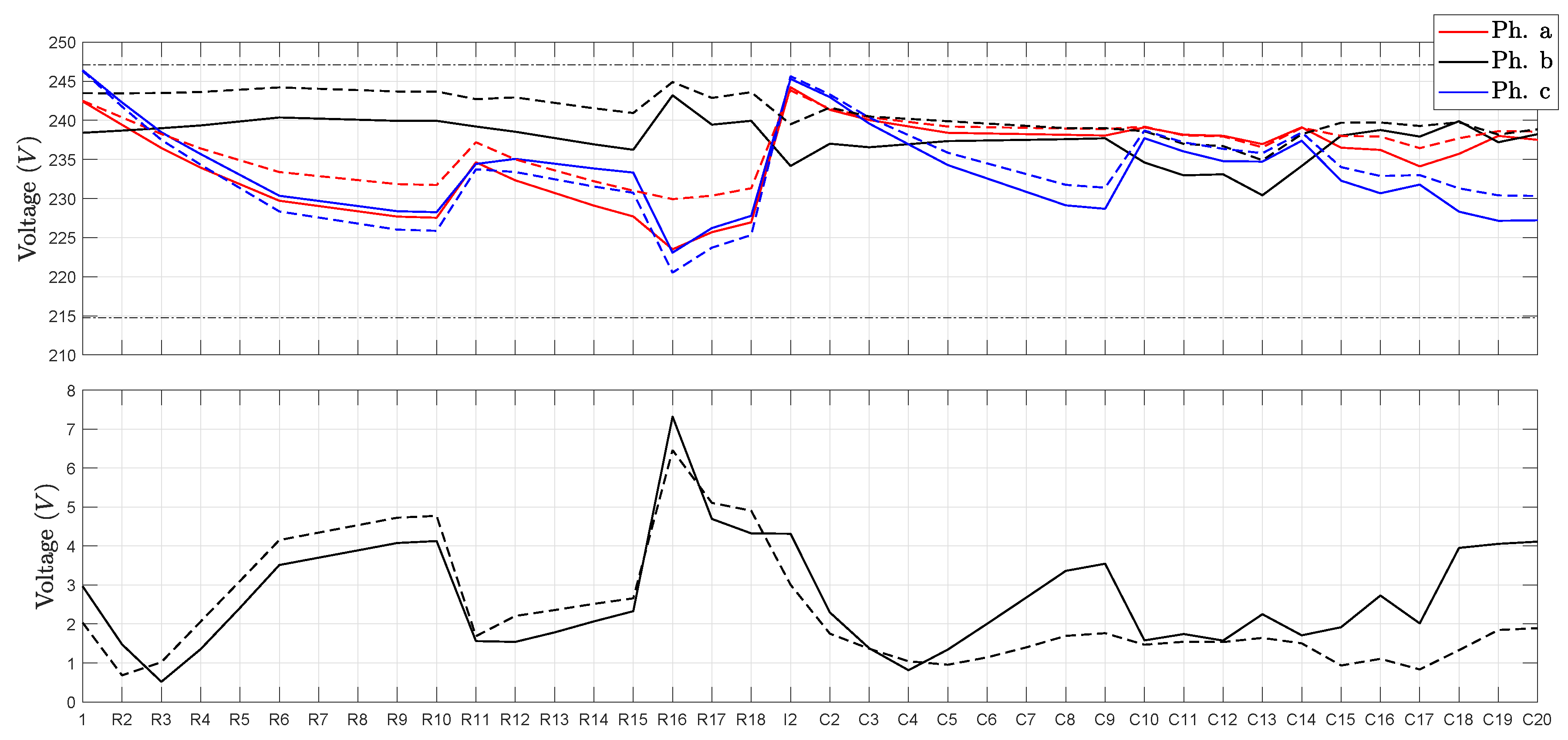
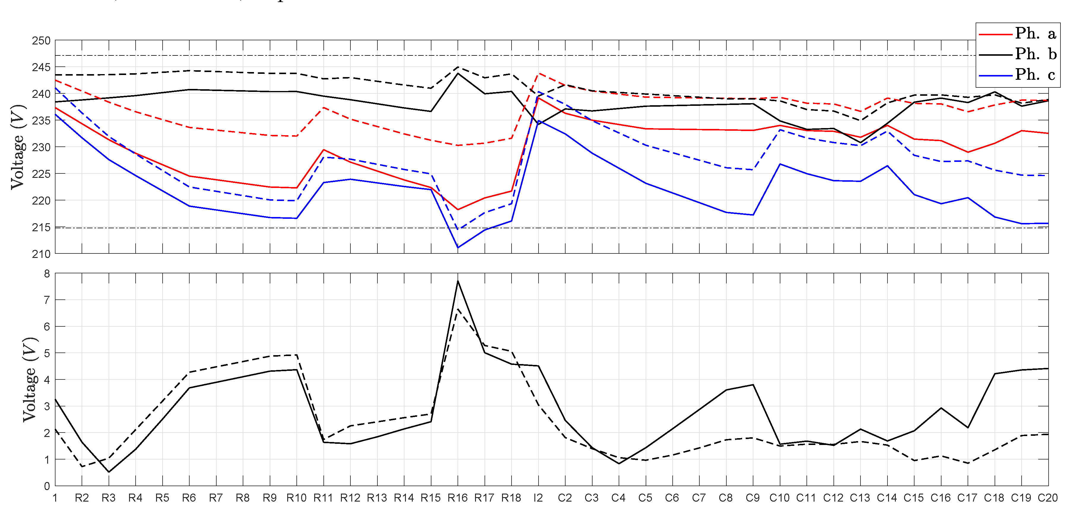
Figure 8 shows the phase-neutral voltages and neutral voltage at all buses for the 1P-OLTCST for both an accurate model and a simplified model of power lines. Figure 9 is the counterpart of Figure 8 for the 3P-OLTCST. It is easily deduced by their comparison that the 1P-OLTCST phase-neutral voltages become more balanced than those reached by the 3P-OLTCST, and the maximum voltage drop is quite a bit lower in the first case, with values of 23.3 V and 32.6 V at the residential feeder for 1P-OLTCST and 3P-OLTCST, respectively. This result is expected because of the improved control flexibility of 1P-OLTCST compared with 3P-OLTCST.

4.3. Ground Configuration

In this second case study, the effects of the neutral ground configuration on the optimal tap positions, system losses, and network voltage values are shown. Let us consider the same load configuration as in the previous section (Table 2) but with different ground resistances.

From

Table 5. Neutral ground resistances at each bus.

Bus	1	R4	R6	R8	R10	R11	R15	R16	R17	R18	I2	C3
$R_g\left(\mathsf{\Omega }\right)$	3	$R_1$	$R_2$	$R_1$	$R_2$	$R_1$	$R_2$	$R_1$	$R_2$	$R_1$	$R_1$	$R_2$
Bus	C5	C7	C9	C11	C12	C13	C14	C16	C17	C18	C19	C20
$R_g\left(\mathsf{\Omega }\right)$	$R_1$	$R_2$	$R_1$	$R_2$	$R_1$	$R_2$	$R_1$	$R_2$	$R_1$	$R_2$	$R_1$	$R_2$

, the sequel ground configurations are analyzed:

• Case 1: Neutral resistor of finite value: $R_1=R_2=40\mathsf{\Omega }$.
• Case 2: Neutral rigid earthing: $R_1=R_2=0\mathsf{\Omega }$.
• Case 3: Neutral resistor of finite value: $R_1=R_2=3\mathsf{\Omega }$.
• Case 4: Mixed earthing: $R_1=40\mathsf{\Omega }$, $R_2=0\mathsf{\Omega }$.

Table 6. Simulation results for different neutral ground configurations.

1P-OLTCST
	Case 1		Case 2		Case 3		Case 4
	1P	3P	1P	3P	1P	3P	1P	3P
	OLTCST	OLTCST	OLTCST	OLTCST	OLTCST	OLTCST	OLTCST	OLTCST
$r_a$	0.94		0.94		0.94		0.94
$r_b$	0.96	0.96	0.94	0.94	0.96	0.96	0.96	0.96
$r_c$	0.92		0.92		0.92		0.92
$P_{loss}\left(W\right)$	19,554.548	21,070.299	18,607.972	19,172.366	19,494.120	21,003.3412	19,201.089	20,673.079
Losses (%)	85.07	91.66	85.23	87.81	85.09	91.67	85.17	91.70
$V_{max}\left(V\right)$	246.386	243.764	246.335	245.358	246.387	243.552	246.376	243.013
$V_{min}\left(V\right)$	223.084	211.088	222.224	216.103	223.182	211.199	222.896	210.921
3P-OLTCST
	Case 1		Case 2		Case 3		Case 4
$r_a$
$r_b$	1		1		1		1
$r_c$
$P_{loss}\left(W\right)$	22,985.288		21,831.880		22,910.126		22,544.249
Losses (%)	100		100		100		100
$V_{max}\left(V\right)$	234.531		230.955		234.310		233.746
$V_{min}\left(V\right)$	200.288		199.543		200.406		200.106

shows the simulation results for the four cases and for both types of control transformers, as well as the solutions for each case when the tap positions remain at their nominal values, for comparison purposes. We highlight that the optimal transformer taps are the same for all cases, except for the one in which a rigid earthing of the neutral is considered (Case 2), and for both types of control transformers. It can be seen that the results for a neutral grounding with a resistor of $3\mathsf{\Omega }$ (Case 3) and a resistor of $40\mathsf{\Omega }$ (Case 1) are very similar. However, only the 1P-OLTCST is able to maintain the voltage within the prescribed limits since the 3P-OLTCST is not able to satisfy voltage limits for any non-null value of grounding resistors. It is also noticeable that the 1P-OLTCST improves the power losses by around a 6% compared with the 3P-OLTCST in almost all cases. This improvement is reduced to 2.5% in the case of rigid grounding.

As in the previous subsection, all these observations strengthen the confirmation of the benefits gained from using decoupled controls and the importance of being rigorous in electrical modeling. In this case, with the earthing configuration, the knowledge of the neutral earthing is needed not only to understand the real state of the system but also to properly solve the voltage optimization problem.

Additionally, in Figure 10, the differences between the bus voltages in Cases 2, 3, and 4 with respect to those of Case 1 are depicted using the 1P-OLTCST. Some noteworthy remarks are as follows: (1) phase-neutral voltages in Case 3 are practically equal to those obtained in Case 1: that is, a ground resistor of 40 $\mathsf{\Omega }$ produces practically the same voltages as those obtained with a ground resistor of 3 $\mathsf{\Omega }$; (2) larger differences occur when a perfectly rigid ground resistance (Case 2) exists, with phase-neutral voltages not as low as those in the case of a non-null ground resistor (Case 1); (3) the final phase-neutral voltages in Case 4 are approximately between the two previous ones.

4.4. Distributed Generation

In the previous sections, some simulations are presented in order to demonstrate the importance of the model when carrying out effective control of the power system and for depicting a realistic load scenario without the presence of renewable generation. If distributed generation is considered, the degree of imbalances is expected to be higher, and the differences shown when considering an accurate or a simplified model of the power lines, together with the improvements introduced by the use of a 1P-OLTCST, can become even greater.

In this subsection, distributed PV generation units that can act as single-phase or three-phase generators with regard to their power capability are installed in some buses of the network. A 24-hour time period, during which load and generation profiles are collected every 15 minutes, is considered in this subsection using profiles obtained from [49]. These profiles are adapted to our problem by scaling them to the maximum power and the power factor detailed in

Table 7. Load/distributed generation configuration.

Bus	R2	R11	R15	R16	R17	R18	I2	C2
$S_{max}\left[kVA\right]$	20	−75	25	−135	17	80	−105	−36
$cos\phi$	0.95	0.95	0.95	0.95	0.95	0.95	0.95	0.95
Ph. a (%)	0	30	0	30	100	$33.33$	30	30
Ph. b (%)	100	40	0	40	0	$33.33$	40	40
Ph. c (%)	0	30	100	30	0	$33.33$	30	30
Bus	C12	C13	C14	C17	C18	C19	C20
$S_{max}\left[kVA\right]$	−101	−36	35	20	−24	−48	−24
$cos\phi$	0.95	0.95	0.95	0.95	0.95	0.95	0.95
Ph. a (%)	30	40	$33.33$	100	30	30	30
Ph. b (%)	40	30	$33.33$	0	40	40	40
Ph. c (%)	30	30	$33.33$	0	30	30	30

. The distribution of load/generation at each of the three phases of every bus is also specified.

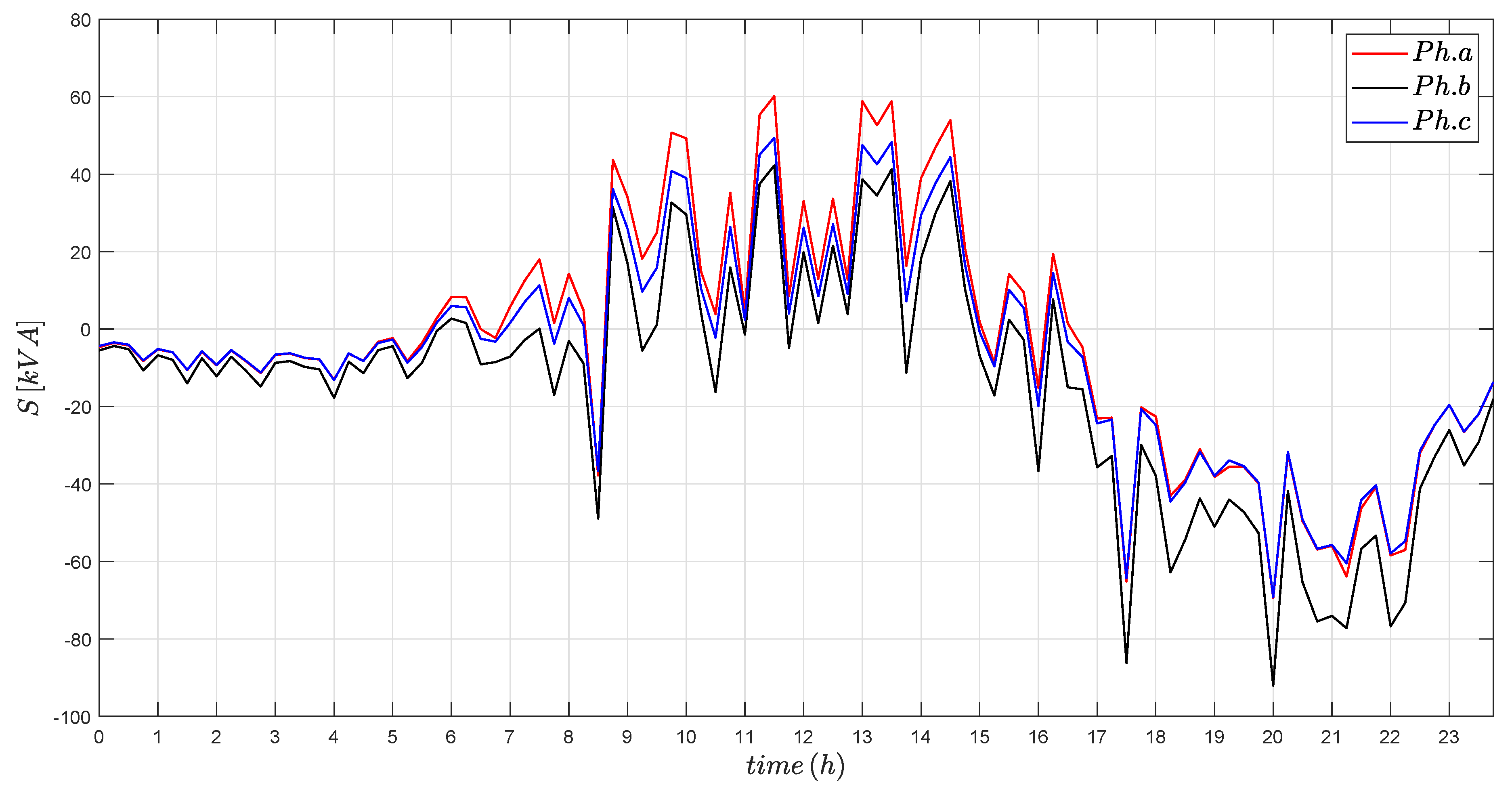
Figure 11 shows the total net apparent power at each hour for the described daily load/generation scenario, so the reader is able to estimate the resulting total imbalances at each time. As expected, the largest imbalances among the three phases are identified as occurring during the hours of highest photovoltaic generation.

The final adopted ground configuration is specified in Table 3.

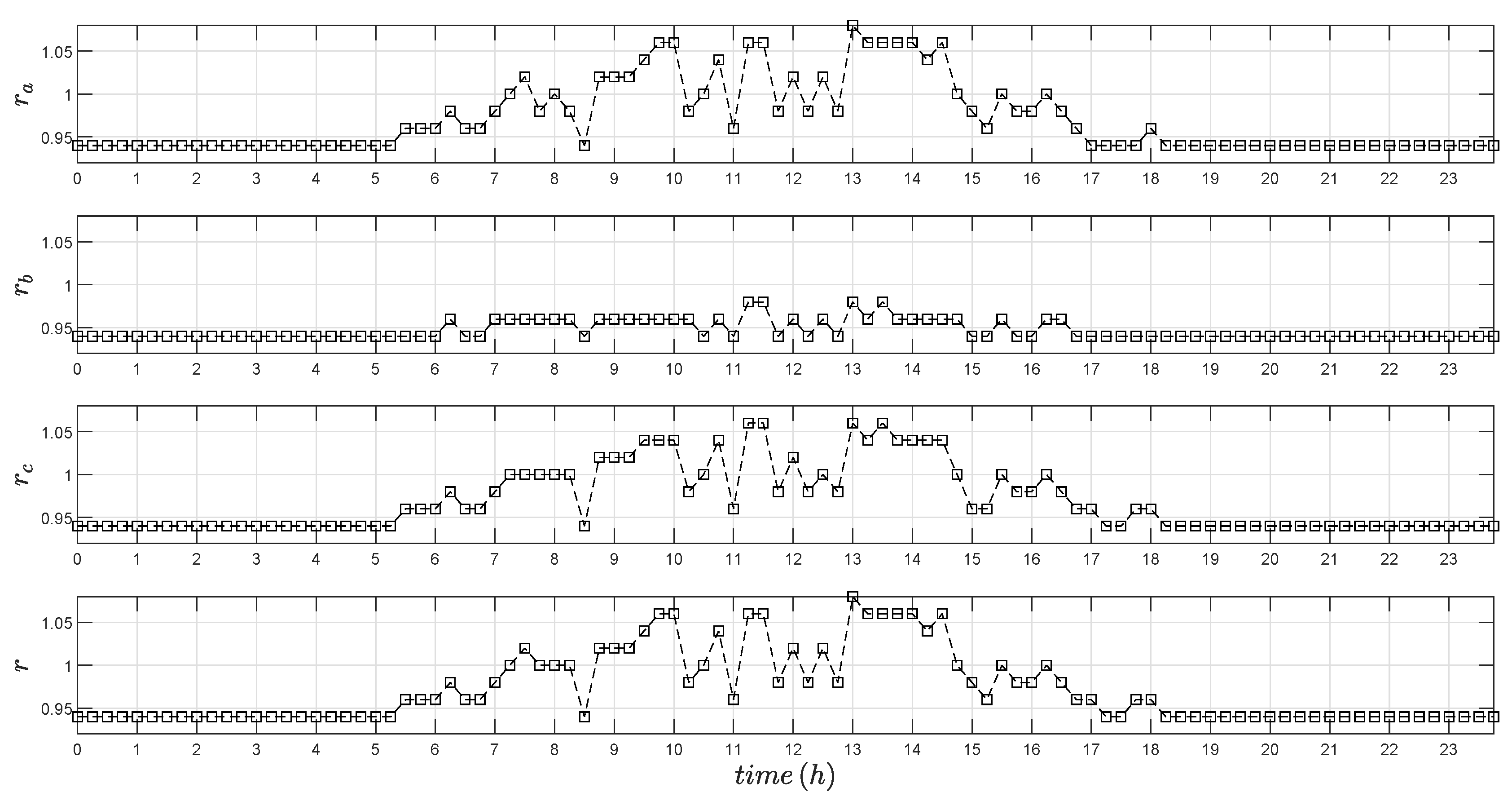
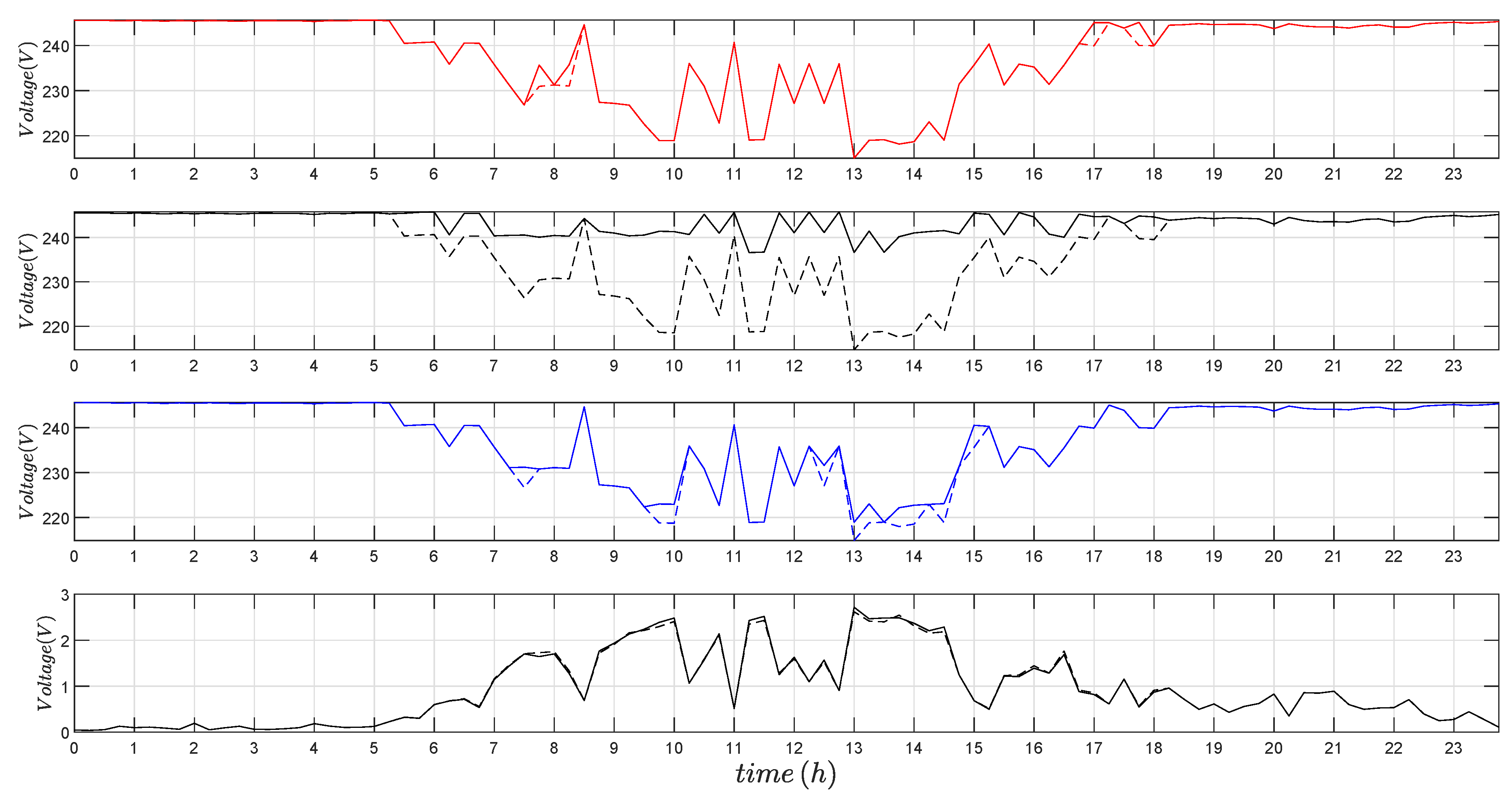
Figure 12 details the obtained optimal tap values when using a 1P-OLTCST or 3P-OLTCST for the specified daily scenario, while Figure 13 shows the evolution of each phase-neutral voltage on the secondary side of the MV/LV transformer. It is easy to identify the numerous times at which the 1P-OLTCST obtains different tap positions for each of the three phases, and it is particularly outstanding for phase b.

In reference to the savings in energy losses, that is, the integral of the objective function reached by the two control strategies, the 1P-OLTCTS results in 3% lower daily losses, while the 3P-OLTCTS saves only 1.05% at the end of the day.

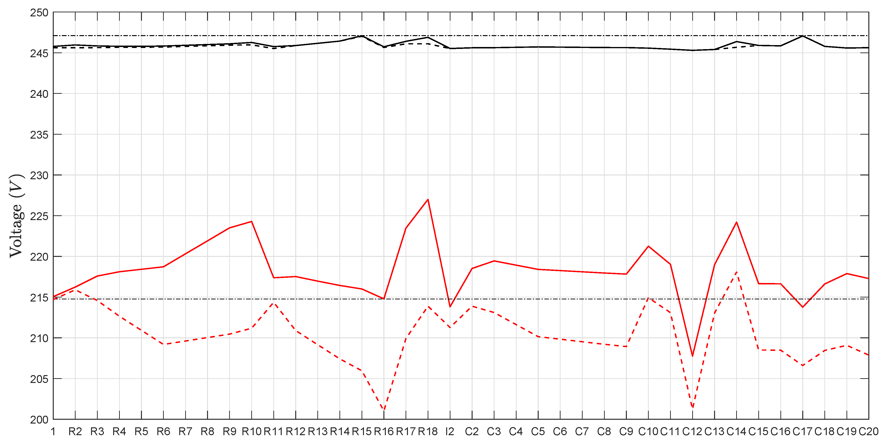
Figure 14 shows the maximum and minimum phase-neutral voltage recorded throughout the day at every bus. It is noticeable that the 1P-OLTCTS has lower min–max voltage differences than those obtained with the 3P-OLTCTS. This means that daily voltage variations at any bus are narrower when decoupled voltage control is considered. It is also apparent that the 3P-OLTCTS is not able to maintain voltages within limits, as it exceeds the lower limits at almost all buses at least once a day.

5. Conclusions and Future Work

This work aimed to study optimal voltage control in low-voltage systems by using transformers with on-load tap changers for two options: the classical OLTC that modifies the transformer ratio and a decoupled OLTC that allows different tap positions at each phase of the three-phase transformer. In contrast with previous research, the associated exact optimization problem was detailed and programmed with a special emphasis on the three-phase modeling of all network components as a requirement due to the unbalanced nature of these systems. The proposed tool was tested on a benchmark low-voltage network under different load and renewable generation scenarios. The main conclusions are as follows:

• Using simplified models for three-phase four-wire lines or excluding considerations of the neutral earthing configuration led to erroneous or suboptimal solutions, regardless of whether 1P-OLTCST or 3P-OLTCST was used. This conclusion was obtained even for low unbalanced scenarios (32.1%, 22.7%, and 44.2%), so we can infer that even worse results would occur with an increase in the level of renewable penetration. This conclusion is quite relevant: simplified models are attractive because of their simplicity, but their use can lead to insecure operation of the system.
• The use of simplified models for three-phase four-wires lines caused an underestimation of the voltage drops in most cases, for either of the two OLTCs considered. The worst identified underestimation reached 10 V.
• Regarding the grounding resistance configuration, two main solutions were obtained. It was observed that when the ground resistance increases above zero, the same optimal tap positions are obtained no matter the resistance value (ground resistances of 3 $\mathsf{\Omega }$ and 40 $\mathsf{\Omega }$ produce almost the same results, but quite different from those corresponding to $R_g=0$$\mathsf{\Omega }$). Conversely, a different solution is reached when rigid ground connection is taken into consideration.
• Decoupled OLTCs are more effective voltage controls than the common OLTC transformers that change the three-phase transformer ratio. It was proven that the 1P-OLTCTS fulfills its primary function of maintaining the voltage within limits most of the time, even in very unbalanced scenarios. This ability is crucial when analyzing networks with high levels of penetration of renewable energy sources. In contrast, the 3P-OLTCTS did not succeed in fulfilling that requirement in many cases. The definition and implementation of the exact optimization problem carried out throughout this work was essential to come to this conclusion and would have not been possible if approximated models had been assumed.
• Besides more effectively maintaining voltage within limits and having lower power losses, the 1P-OLTCTS had lower voltage drops and daily voltage variation than the 3P-OLTCTS. For the tested cases, the best saving in power losses was 85.1% for the 1P-OLTCTS, versus 91.7% for the 3P-OLTCTS; the highest voltage drop was 4.5% for the 1P-OLTCTS, versus 9% for the 3P-OLTCTS; and the maximum daily voltage variation was reduced by up to more than 10 V with 1P-OLTCTS versus 3P-OLTCTS.

Future work will examine the coupling of all time frameworks under study in order to reduce the number of movements of tap positions and to maximize the lifetime of the device; it is clear that such tap movements do not lead to profitable savings of power losses and although voltages are within limits, tap movements should be avoided. In addition, the current work focused on the decoupled OLTC as the only means of voltage control in order to understand its real possibilities and because it is a solution that is close to the current reality of utilities. However, additional voltage controls, such as statcoms, inverters linked to renewable generators, or storage systems, would be interesting to study in future analyses.

References

- Country Fiches for Electricity Smart Metering Accompanying the Document Report from the Commission Benchmarking Smart Metering Deployment in the EU-27 with a Focus on Electricity; Commission Staff Working Document; Publications Office of the European Union: Brussels, Belgium, 2014.
- International Energy Agency (IEA). IRENA Cost and Competitiveness Indicators: Rooftop solar PV; IEA Publications: Paris, France, December 2017. [Google Scholar]
- International Energy Agency (IEA). Global EV Outlook 2017. Two Milllion and Counting; IEA Publications: Paris, France, 2017. [Google Scholar]
- Gozel, T.; Ochoa, L.F. Deliverable 3.3 (Updated) Performance evaluation of the monitored LV networks. In Electricity North West Limited (ENWL)—Low Voltage Network Solutions; The University of Manchester: Manchester, UK, July 2014. [Google Scholar]
- Mohammadi, P.; Mehraeen, S. Challenges of PV Integration in Low-Voltage Secondary Networks. IEEE Trans. Power Deliv. 2017, 32, 525–535. [Google Scholar]
- Noske, S.; Falkowski, D.; Swat, K.; Boboli, T. UPGRID project: The management and control of LV network. CIRED-Open Access Proc. J. 2017, 2017, 1520–1522. [Google Scholar] [CrossRef]
- Poursharif, G.; Brint, A.; Black, M.; Marshall, M. Analysing the ability of smart meter data to provide accurate information to the UK DNOs. CIRED-Open Access Proc. J. 2017, 2017, 2078–2081. [Google Scholar] [Green Version]
- Wong, P.K.C.; Barr, R.; Kalam, A. Analysis of voltage quality data from smart meters. In Proceedings of the 22nd Australasian Universities Power Engineering Conference (AUPEC), Bali, Indonesia, 26–29 September 2012. [Google Scholar]
- Wong, P.K.C.; Barr, R.; Kalam, A. A big data challenge—Turning smart meter voltage quality data into aionable information. In Proceedings of the 22nd International Conference on Electricity Distribution (CIRED), Stockholm, Sweden, 10–13 June 2013. [Google Scholar]
- Prado, J.G.; González, A.; Riaño, S. Adopting smart meter events as key data for low-voltage network operation. CIRED-Open Access Proc. J. 2017, 2017, 924–928. [Google Scholar] [CrossRef] [Green Version]
- Navarro, A.; Ochoa, L.F.; Mancarella, P.; Randles, D. Impacts of photovoltaics on low voltage networks: A case study for the North West of England. In Proceedings of the 22nd International Conference on Electricity Distribution (CIRED), Stockholm, Sweden, 10–13 June 2013. [Google Scholar]
- Report C1: Use of smart meter information for network planning and operation. In UK Power Networks Holdings Limited—Low Carbon London Project; UK Power Networks Holdings Limited: London, UK, September 2014.
- Seymour, J.; The Seven Types of Power Problems. White Paper 18, Revision 1, Schneider Electric—Data Center, Science Center. 2011. Available online: http://www.apc.com/salestools/VAVR-5WKLPK/VAVR-5WKLPK_R 1_EN.pdf (accessed on 1 May 2019).
- O’Connell, A.; Soroudi, A.; Keane, A. Distribution Network Operation Under Uncertainty Using Information Gap Decision Theory. IEEE Trans. Smart Grid 2018, 9, 1848–1858. [Google Scholar]
- Lan, B.-R.; Chang, C.-A.; Huang, P.-Y.; Kuo, C.-H.; Ye, Z.-J.; Shen, B.-C.; Chen, B.-K. Conservation voltage regulation (CVR) applied to energy savings by voltage-adjusting equipment through AMI. IOP Conf. Ser. Earth Environ. Sci. 2017, 93, 012070. [Google Scholar] [CrossRef]
- Nijhuis, M.; Gibescu, M.; Cobben, J.F.G. Valuation of measurement data for low voltage network expansion planning. Electr. Power Syst. Res. 2017, 151, 59–67. [Google Scholar] [CrossRef]
- Aziz, T.; Ketjoy, N. PV Penetration Limits in Low Voltage Networks and Voltage Variations. IEEE Access 2017, 5, 16784–16792. [Google Scholar]
- Tahir, M.; Nassar, M.E.; El-Shatshat, R.; Salama, M.M.A. A review of Volt/Var control techniques in passive and active power distribution networks. In Proceedings of the 4th IEEE International Conference on Smart Energy Grid Engineering (SEGE), Oshawa, ON, Canada, 21–24 August 2016; pp. 57–63. [Google Scholar]
- Bayer, B.; Matschoss, P.; Thomas, H.; Marian, A. The German experience with integrating photovoltaic systems into the low-voltage grids. Renew. Energy 2018, 119, 129–141. [Google Scholar] [CrossRef]
- Yan, R.; Marais, B.; Saha, T.K. Impacts of residential photovoltaic power fluctuation on on-load tap changer operation and a solution using DSTATCOM. Electr. Power Syst. Res. 2014, 111, 185–193. [Google Scholar] [CrossRef]
- Long, C.; Ochoa, L.F. Voltage Control of PV-Rich LV Networks: OLTC-Fitted Transformer and Capacitor Banks. IEEE Trans. Power Syst. 2016, 31, 4016–4025. [Google Scholar] [CrossRef]
- Coppo, M.; Turri, R.; Marinelli, M.; Han, X. Voltage management in unbalanced low voltage networks using a decoupled phase-tap-changer transformer. In Proceedings of the 49th International Universities Power Engineering Conference (UPEC), Cluj-Napoca, Romania, 2–5 September 2014; pp. 1–6. [Google Scholar]
- Zecchino, A.; Marinelli, M.; Hu, J.; Coppo, M.; Turri, R. Voltage control for unbalanced low voltage grids using a decoupled-phase on-load tap-changer transformer and photovoltaic inverters. In Proceedings of the 50th International Universities Power Engineering Conference (UPEC), Stoke on Trent, UK, 1–4 September 2015; pp. 1–6. [Google Scholar]
- Hu, J.; Marinelli, M.; Coppo, M.; Zecchino, A.; Bindner, H.W. Coordinated voltage control of a decoupled three-phase on-load tap changer transformer and photovoltaic inverters for managing unbalanced networks. Electr. Power Syst. Res. 2016, 131, 264–274. [Google Scholar] [CrossRef] [Green Version]
- Zecchino, A.; Hu, J.; Coppo, M.; Marinelli, M. Experimental testing and model validation of a decoupled-phase on-load tap-changer transformer in an active network. IET Gen. Transm. Distrib. 2016, 10, 3834–3843. [Google Scholar] [CrossRef]
- Quirós-Tortós, J.; Ochoa, L.F.; Alnaser, S.W.; Butler, T. Control of EV Charging Points for Thermal and Voltage Management of LV Networks. IEEE Trans. Power Syst. 2016, 31, 3028–3039. [Google Scholar] [CrossRef]
- Efkarpidis, N.; Rybel, T.D.; Driesen, J. Optimal Placement and Sizing of Active In-Line Voltage Regulators in Flemish LV Distribution Grids. IEEE Trans. Ind. Appl. 2016, 52, 4577–4584. [Google Scholar] [CrossRef]
- Procopiou, A.T.; Ochoa, L.F. Voltage Control in PV-Rich LV Networks Without Remote Monitoring. IEEE Trans. Power Syst. 2017, 32, 1224–1236. [Google Scholar] [CrossRef]
- Pezeshki, H.; Arefi, A.; Ledwich, G.; Wolfs, P. Probabilistic Voltage Management Using OLTC and dSTATCOM in Distribution Networks. IEEE Trans. Power Deliv. 2017, 33, 570–580. [Google Scholar] [CrossRef]
- Fallahzadeh-Abarghouei, H.; Nayeripour, M.; Hasanvand, S.; Waffenschmidt, E. Online hierarchical and distributed method for voltage control in distribution smart grids. IET Gen. Transm. Distrib. 2017, 11, 1223–1232. [Google Scholar] [CrossRef]
- Aziz, T.; Ketjoy, N. Enhancing PV Penetration in LV Networks Using Reactive Power Control and On Load Tap Changer with Existing Transformers. IIEEE Access 2018, 6, 2683–2691. [Google Scholar] [CrossRef]
- Bettanin, A.; Coppo, M.; Savio, A.; Turri, R. Voltage management strategies for low voltage networks supplied through phase-decoupled on-load-tap-changer transformers. In Proceedings of the AEIT International Annual Conference, Cagliari, Italy, 20–22 September 2017; pp. 1–6. [Google Scholar]
- Jiricka, J.; Kaspirek, M.; Kolar, L.; Zahradka, M. Smart Substation MV/LV. In Proceedings of the 24th International Conference on Electricity Distribution (CIRED), Glasgow, UK, 12–15 June 2017; pp. 1–5. [Google Scholar]
- Baudot, C.; Roupioz, G.; Carre, O.; Wild, J.; Potet, C. Experimentation of voltage regulation infrastructure on LV network using an OLTC with a PLC communication system. CIRED-Open Access Proc. J. 2017, 2017, 1120–1122. [Google Scholar] [CrossRef] [Green Version]
- Mokkapaty, S.; Weiss, J.; Schalow, F.; Declercq, J. New generation voltage regulation distribution transformer with an on load tap changer for power quality improvement in the electrical distribution systems. CIRED-Open Access Proc. J. 2017, 2017, 784–787. [Google Scholar] [CrossRef] [Green Version]
- Daratha, N.; Das, B.; Sharma, J. Coordination Between OLTC and SVC for Voltage Regulation in Unbalanced Distribution System Distributed Generation. IEEE Trans. Power Syst. 2014, 29, 289–299. [Google Scholar] [CrossRef]
- Frame, D.; Bell, K.; McArthur, S. A Review and Synthesis of the Outcomes from Low Carbon Networks Fund Projects. UKERK Publications. August 2016. Available online: http://www.ukerc.ac.uk/publications/ a-review-and-synthesis-of-the-outcomes-from-low-carbon-networks-fund-projects.html (accessed on 1 May 2019).
- Chen, T.-H.; Yang, W.-C. Analysis of multi-grounded four-wire distribution systems considering the neutral grounding. IEEE Trans. Power Deliv. 2001, 16, 710–717. [Google Scholar] [CrossRef]
- Urquhart, A.J. Accuracy of Low Voltage Electricity Distribution Network Modelling. Ph.D. Thesis, Loughborough Universtiy, Loughborough, UK, 2016. [Google Scholar]
- Willis, H.L. Power Distribution Planning Reference Book, 2nd ed.; CRC Press: Boca Raton, FL, USA, March 2004; ISBN 978-0824748753. [Google Scholar]
- Özkan, Z.; Hava, A.M. Three-phase inverter topologies for grid-connected photovoltaic systems. In Proceedings of the International Power Electronics Conference (IPEC), Hiroshima, Japan, 18–21 May 2014; pp. 498–505. [Google Scholar]
- Moreno-Díaz, L.; Romero-Ramos, E.; Gómez-Expósito, A.; Cordero-Herrera, E.; Rivero, J.R.; Cifuentes, J.S. Accuracy of Electrical Feeder Models for Distribution Systems Analysis. In Proceedings of the International Conference on Smart Energy Systems and Technologies (SEST), Sevilla, Spain, 10–12 September 2018; pp. 1–6. [Google Scholar]
- Chen, M.S.; Dillon, W.E. Power system modeling. Proc. IEEE 1974, 62, 901–915. [Google Scholar] [CrossRef]
- Rodas, R.D.E.; Padilha-Feltrin, A.; Ochoa, L.F. Distribution transformers modeling with angular displacement: Actual values and per unit analysis. SBA Controle & Automação Sociedade Brasileira de Automatica 2007, 18, 499–500. [Google Scholar]
- Carneiro, S.; Martins, H.J.A. Measurements and model validation on three-phase core-type distribution transformers. In Proceedings of the IEEE Power Engineering Society General Meeting, Toronto, ON, Canada, 13–17 March 2004; pp. 120–124. [Google Scholar]
- Kersting, W.H. Distribution System Modeling and Analysis, 3rd ed.; CRC Press: Boca Raton, FL, USA, February 2016. [Google Scholar]
- Modelling and Aggregation of Loads in Flexible Power Networks; Working Group C4.605; CIGRÉ, Conseil International des Grands Réseaux éLectriques: Paris, France, February 2014.
- Benchmark Systems for Network Integration of Renewable and Distributed Energy Resources; Comité d’études C6; CIGRÉ, Conseil international des grands réseaux électriques: Paris, France, 2014.
- Gozel, T.; Navarro, A.; Ochoa, L.F. Deliverable 3.5 Creation of Aggregated Profiles with and without New Loads and DER Based on Monitored Data. April 2014. Available online: https://www.enwl.co.uk/zero-Carbon/smaller (accessed on 1 May 2019).
Figure 1.
Schema of a common European low-voltage (LV) network.
Figure 2.
Thévenin equivalent for a medium-voltage (MV) grid.
Figure 3.
Equivalent circuit for a single-phase transformer.
Figure 4.
yg three-phase transformer.
Figure 5.
Three-phase four-wire electric line model.
Figure 6.
Example of three-phase wye (a and b) and delta (c) loads/renewable generators at bus i.
Figure 7.
Modified European low-voltage benchmark network [48].
Figure 8.
Simulation results when considering a 1P-OLTCST for both the accurate model and simplified model (dashed lines) of power lines.
Figure 9.
Simulation results when considering a 3P-OLTCST for both the accurate model and simplified model (dashed lines) of power lines.
Figure 10.
Differences between the phase-neutral and neutral bus voltages in Cases 2, 3, and 4 with respect to Case 1.
Figure 11.
Net total apparent power at the MV/LV transformer without considering losses.
Figure 12.
Optimal tap positions when considering a 1P-OLTCTS or 3P-OLTCTS.
Figure 13.
Phase-neutral voltage evolution for bus R1 when considering a 1P-OLTCTS or 3P-OLTCTS (dashed lines) for phases a, b, and c and neutral voltage.
Figure 14.
Maximum and minimum phase-neutral voltage at every bus for both the 1P-OLTCTS and 3P-OLTCTS (dashed lines).