Estimation of the Daily Variability of Aggregate Wind Power Generation in Alberta, Canada


1
Department of Mathematics and Statistics, University of Calgary, 2500 University Dr NW, Calgary, AB T2N 1N4, Canada
2
Department of Mechanical and Manufacturing Engineering, University of Calgary, 2500 University Dr NW, Calgary, AB T2N 1N4, Canada
3
Department of Electrical and Computer Engineering, University of Calgary, 2500 University Dr NW, Calgary, AB T2N 1N4, Canada
*
Author to whom correspondence should be addressed.
†
These authors contributed equally to this work.
Energies 2019, 12(10), 1998; https://doi.org/10.3390/en12101998
Submission received: 24 March 2019
/
Revised: 30 April 2019
/
Accepted: 15 May 2019
/
Published: 24 May 2019
Abstract
:This paper describes a hierarchy of increasingly complex statistical models for wind power generation in Alberta applied to wind power production data that are publicly available. The models are based on combining spatial and temporal correlations. We apply the method of Gaussian random fields to analyze the wind power time series of the 19 existing wind farms in Alberta. Following the work of Gneiting et al., three space-time models are used: Stationary, Separability, and Full Symmetry. We build several spatio-temporal covariance function estimates with increasing complexity: separable, non-separable and symmetric, and non-separable and non-symmetric. We compare the performance of the models using kriging predictions and prediction intervals for both the existing wind farms and a new farm in Alberta. It is shown that the spatial correlation in the models captures the predominantly westerly prevailing wind direction. We use the selected model to forecast the mean and the standard deviation of the future aggregate wind power generation of Alberta and investigate new wind farm siting on the basis of reducing aggregate variability.
1. Introduction
This study focuses on the wind power system of Alberta, Canada. Wind plays an increasingly important role in the energy system of Alberta. Since the first commercial wind farm was built in southern Alberta in 1993, the government of Alberta has continued to support the development of wind power. Currently, the wind energy capacity in Alberta is 1479 MW, ranking third in Canada, but the government expects to at least triple the current wind power capacity by 2030 [1]. This motivates us to find an efficient model to forecast the future performance of the current wind energy grid and the potential generation of new wind farms in Alberta. Our goal is to predict the aggregate wind power generation in Alberta in the future with the further goals of analyzing congestion of the power grid, the best locations of future wind farms, and the relationship between wind and solar power. In particular, our study could help to better understand the smoothing effect of [2,3] hybrid wind and solar energy systems on the future overall renewable production patterns in Alberta.
We aim to explore the quantitative and qualitative insights regarding wind energy production in a geographical region using publicly available data. Wind resource estimation by wind power developers and others involved in the wind power system is an expensive undertaking. It is helpful for the stakeholders to know what can be done with public data and open software so that they can use wind resource estimation more strategically, for example, for high-level critical analysis of a few selected sites.
Wind speed is the most relevant factor related to wind power. In particular, the wind power curves for different types of wind turbines have roughly the same shape [4], hence one approach to modeling wind power is to model the wind speed and associate it to the wind power. Wind speed can be modeled as a spatio-temporal process as it evolves randomly in time and space. Second order models are one of the most basic types of spatio-temporal processes used in the modeling of wind. They use the spatio-temporal covariance as a basis for estimation and are most suitable when the underlying process can be modeled as a Gaussian spatio-temporal field. Gneiting et al. [5] applied this approach to model Irish wind data. In particular, under the assumption of stationarity, they consider various parametric covariance function models with increasing complexity: separable, non-separable but symmetric, and finally non-symmetric and non-separable. Non-separable and non-symmetric covariance function models have proved useful for the modeling of wind. For example, Gneiting et al. [5] incorporate well-known wind patterns of Ireland using such covariance functions.
In this paper, we apply the covariance function models used in [5] to a new data set, namely the wind power generation data of Alberta, Canada. We enhance their methodology by obtaining kriging prediction intervals, in addition to kriging point predictions. We use the mean percentage of observations outside the kriging prediction intervals as a performance measure additional to the mean square error (MSE) and the mean absolute error (MAE) used in [5]. Moreover, we perform kriging predictions after excluding one wind farm. That is, we leave out the historical data of one site in the estimation of the models. Thereafter, we use the estimated models and the information of the other sites to predict the observations at the excluded site. We use the error of these predictions as a performance measure for the models to predict the wind power outputs at future sites. Finally, we derive the distribution of the future aggregate power production using the planned site and capacity information of the future wind farms in Alberta. The main incentive for this is that increasing renewable energy generation tends to depress the wholesale price of electricity. Thus, a new farm that reduces the variability of aggregate wind power may well be financially attractive even if its capacity factor is relatively low.
1.1. Other Modeling Methodologies
There are many studies in the literature on wind power forecasting, but few of them consider both spatial and temporal dimensions.
Chen et al. [6] predict the wind speed data at a single wind farm by correcting the numerical weather prediction (NWP) using a Gaussian process (GP); they then model the relationship between the corrected wind speed and power output using a censored Gaussian process.Ma et al. [7] model the power output of a single farm at multiple time lags as a multivariate normal distribution after a non-parametric transformation of the wind power data using the inverse of the empirical distribution function of wind power. Yang et al. [8] use support vector machines (SVM) to predict the wind power time series at the individual sites and use a Gaussian copula to model the forecast error at the multiple sites; they then apply the methodology to three adjacent wind farms. Li et al. [9] combines NWP with a wind power curve model to predict the wind power at an individual site and use a Gaussian copula to model the prediction error at multiple sites. Gneiting et al. [10] and Hering and Genton [11] build a more complex model of the interaction of the wind speeds at multiple sites by expressing the parameters of the conditional distribution of the wind speed at a future time point as a linear function of current or past observations of other sites. This linear function is altered according to a regime switching process which mimics the alternating wind patterns observed in the geographical region. Cavalcante et al. [12] use vector autoregression (VAR) to model the time series of wind speeds of multiple farms and apply the least absolute shrinkage and selection operator (LASSO) for variable selection. Browell et al. [13] combine VAR with a regime switching process, where the regimes are determined by NWP. There are many other studies of a similar nature to the ones just described, e.g., Damousis et al. [14,15]; however, none of these methodologies model the wind speed/power in a geographical region as a spatio-temporal process, hence the forecasts can only be obtained for the sites for which the historical data are available. In addition, while all these studies model the correlation between different sites, they do not build a unifying covariance structure for the entire region as a function of spatio-temporal separation.
Malvaldi et al. [16] studied the relationship between correlation of the power output of European countries and distance and time lag, which can be viewed as a step towards a spatio-temporal modeling of wind power. Gneiting et al. [5] describe the first use of a second order spatio-temporal process to model the wind speed, incorporating a non-separable covariance function to capture the effect of prevalent wind directions in wind speed. The effect of the prevailing wind direction shows itself through an asymmetry in correlation with respect to positive and negative distances and times, which necessitates the use of non-separable covariance functions, Gneiting [17]. If the wind speed has multiple prevailing directions, the asymmetry is harder to measure; Ezzat et al. [18] develop a more accurate way of measuring the effect of prevailing wind directions by detecting change points in the asymmetry patterns.
1.2. Applications
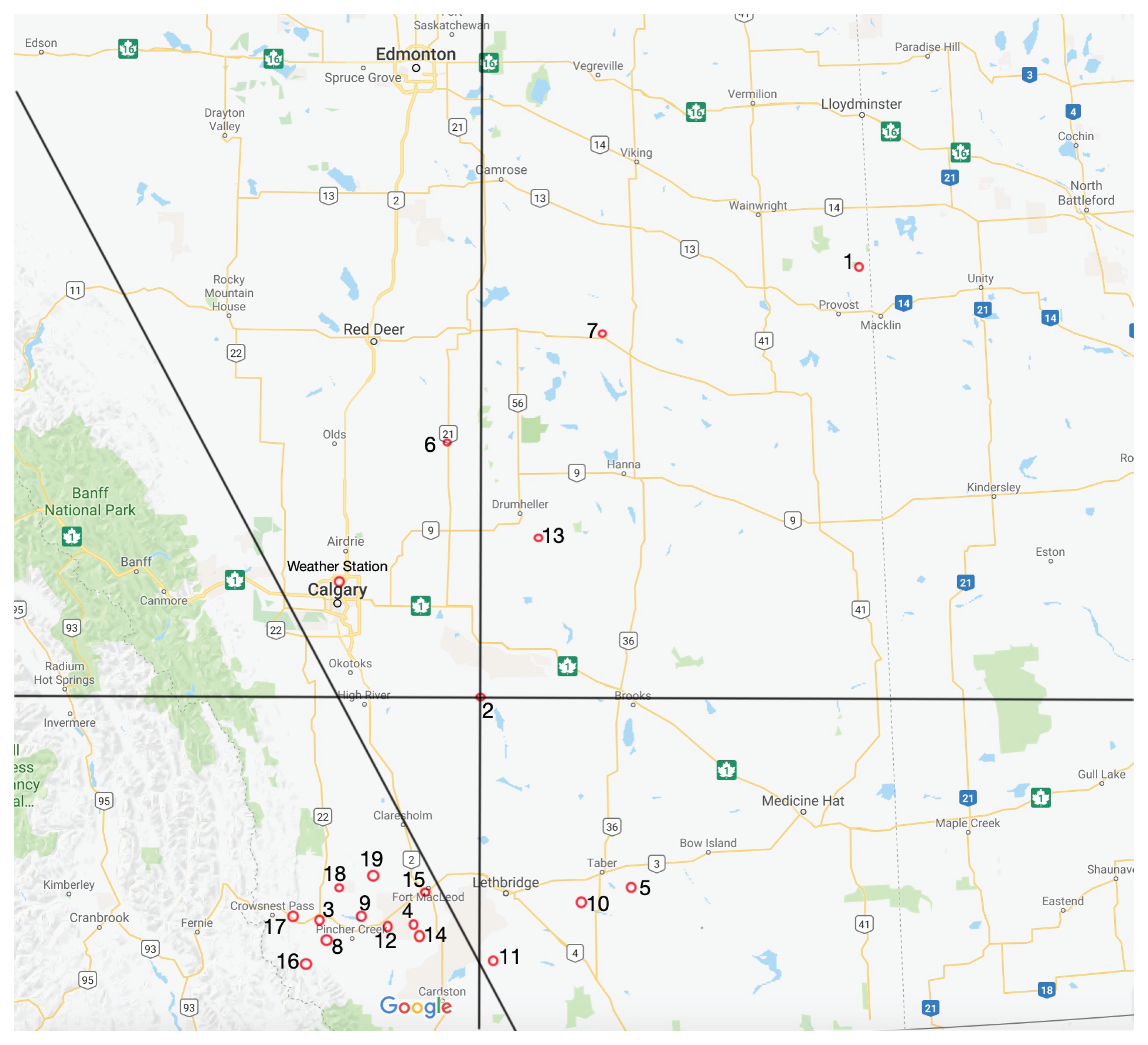
There is also a large amount of literature on the effects of geographic dispersion on aggregate wind power. Reichenberg et al. [19] considered Europe as whole with an assumed rather than actual arrangement of wind farms. They showed that it was possible to optimize the layout to minimize, for example, occurrences of low aggregate power. Tejeda et al. [20] used the reduction in variation of aggregate power to determine ideal sites for further expansion of wind energy in Europe. Malvaldi et al. [16] also considered Europe as a whole with emphasis on the role of interconnections, which are not significant in Alberta whose future scenarios were modeled by MacCormack et al. [21] using simple autocorrelation models. Miettinen and Holttinen [22] considered the errors in day-ahead forecasting for aggregate wind power in another large region, the Nordic countries. Correlations of forecast errors decrease to zero at separations of around 500 km. The errors eventually “saturate”, implying that there is an essential minimum error for any modeling methodology. Most wind farms in Alberta are in the high wind regimes downwind of the Rocky Mountains (the area below the slanted straight line in Figure 1). This clustering influences the variability in aggregate power, which has market and system operation consequences. For example, the wind farms in close proximity produce highly correlated wind power, which usually reduces the wholesale price of electricity during high winds, so that wind farm profits are reduced. On the other hand, a wind farm that is remote from other wind farms may produce power when the other farms do not, and may benefit from selling power at a higher price even if its capacity factor is not as high as the clustered farms. Hence, there are diminishing returns in building a farm near others in high wind regimes. Modeling the joint power production of wind farm clusters is a first step to analyzing the trade off between the wind production potential of a site and the proximity of the site to the other wind farms. To our knowledge, this has not been attempted previously.
2. Wind Energy Generation Data
This study is based on data obtained from the Alberta Electric System Operator (AESO), consisting of wind power production values in megawatts (MW) averaged over one hour periods from January 2016 to December 2017 for 19 wind farms in Alberta. The number of farms was constant over those two years.
The following modifications were made to the data: Two wind farms were very close in distance and belong to the same company, so we combined these two farms as one, labeled as BUL. The next correction is removing the observations on 29 February in 2016 which is a leap year, to avert its influence in seasonality. Additionally, the data of the second hour in 13 March in both 2016 and 2017 were missing. We assumed that there is no dramatic change in an hour in wind power, so we used the average of the wind production in the first and the third hour to estimate the missing value in the second hour.
The farms are identified in Table 1 along with their capacities and shown on the map of Alberta in Figure 1. The horizontal and the vertical black lines represent the x and y axes of our co-ordinate system of the wind farms with the origin at the geographical centre of the farms. The slanted black line separates two distinct regions. The region below the line is subject to strong winds associated with Rocky Mountains which extend from just west of farm number 17 to the Banff National Park. The remainder of the region in Figure 1 is flat. There is a significant cluster of wind farms in this area, and the variability of the wind power generation of these farms is higher than the farms on the right of the line, as shown by the specific variances in the third row of Table 1. The variance for each farm is calculated as the variance of the time series corresponding to that farm after the preprocessing.
Data Preprocessing
To evaluate the out-of-sample prediction performance used in modeling, we separate the data into two sets: the data in 2016 as the training set and the data in 2017 as the testing set.
The histogram of hourly wind power generation in megawatts of each of the 19 wind farms over the training period is given in Figure 2. These histograms indicate that for every wind farm except farm CRE3, the probability distribution function of hourly wind generation shows two visible modes, the biggest one is at zero power, and the other is near maximum capacity. The mode at maximum capacity occurs when all turbines are operating at their rated power. Similarly, the mode at 0 indicates that the wind speed is below the cut-in speed for all turbines. The shape of the histograms is similar to that obtained from the power curve of a single turbine combined with a Weibull or Rayleigh distribution for the wind speed. More precisely, it can be argued that the wind power approximately follows a truncated three-parameter Weibull distribution, since wind speed can be modeled using a two-parameter Weibull distribution, and a simple representation of the power curve as a function of wind speed, U, has the form
where and are the cut-in and rated wind speeds, respectively. Even this simple form implies that a Gaussian model is difficult to justify. In particular, the truncation at cut-in and rated power results in a mixed distribution for power with non-zero probabilities at those conditions. Truncation can be addressed effectively in a Bayesian framework. For example, truncation arises in the modeling of precipitation and several authors model precipitation data as censored observations of a latent Gaussian random field such as Baxevani and Lennartson [23], Glaseby et al. [24], and Allcroft and Glaseby [25] who use the Bayesian methodology to estimate their models. This is also a promising methodology for the wind power data. However, as a result of the computational complexity of the Bayesian approach, we use a simpler alternative in this work. Namely, we transform our data to daily averages which softens the effects of truncation. Thereafter, we divide each data point by the corresponding capacity to obtain a uniform scale across the farms. The resulting data are skewed to the right; we fix that by applying a power transform. We found that a square root transform gave reasonably symmetric histograms overall. Another possibility is to use a transformation based on the quantile function of the three-parameter Weibull distribution; however, we prefer the square-root transform due to its simplicity, enabling us to find explicit formulas for the mean and the variance of aggregate power, see Section 5.
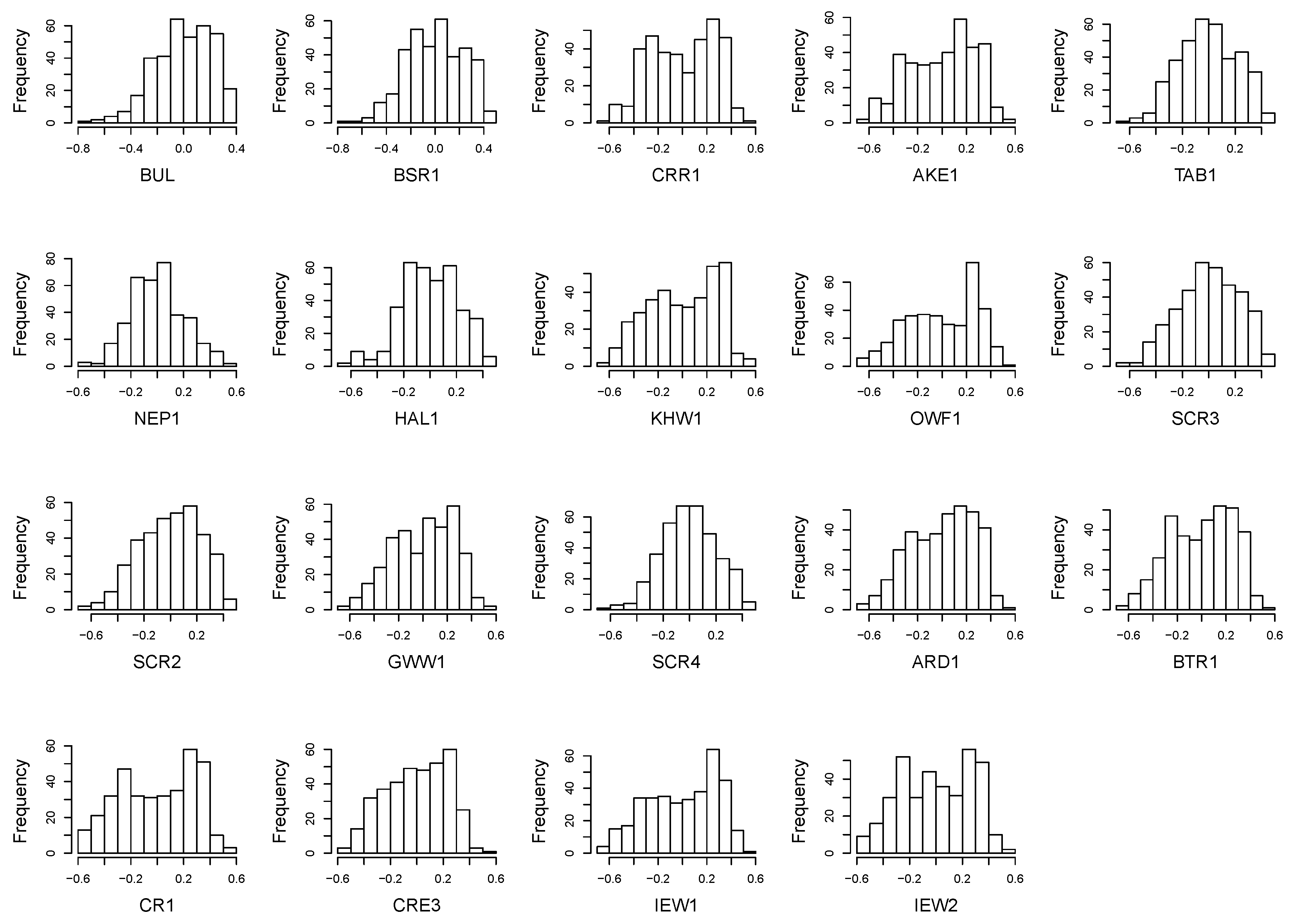
Next, we subtract the seasonal component to obtain a stationary time series for each wind farm. To estimate the seasonal component, we use the locally weighted smoothing estimator (LOWESS, see e.g., Cleveland [26]), a common technique used to discover the trend of variables in a time plot or scatter plot by creating a smooth line. After adjusting for seasonality, we subtract the location-specific mean for each wind farm to get a time series with mean zero. The histograms of preprocessed hourly wind power production values of 19 farms in the training set are plotted in Figure 3, and the flow chart used for the preprocessing is given in Figure 4. Compared with the hourly data histograms, the proportion of observations with no power are significantly reduced in the histograms of the preprocessed data.
3. Modeling
We assume that the preprocessed data correspond to discrete measurements of a Gaussian spatio-temporal process . S is a subset of corresponding to the geographical region containing the 20 wind farms and possible locations for future farms. We assume that , for some function . We also assume that there exists a function , called the correlation function, such that . Our goal is to uncover and C from the data.
To estimate , we use the station specific variances given in Table 1. We group the farms into two groups according to the similarity in their variance. The farms below the split line in Figure 1 have an average station specific variance of 0.07, and the farms above the split line have an average station specific variance of 0.05. Hence, we assume that is of the form:
Because C must be positive definite, an effective strategy is to use a parametric family known to be positive definite. We follow the approach of Gneiting et al. [5] and use three parametric families, where each one is embedded in the next, thus allowing us to introduce increasing complexity at each step. We start with a separable parametric family, then consider a larger symmetric family which is non-separable in general but includes the separable family as a special case. Finally, we consider a convex combination of the second family and a Lagrangian family which is antisymmetric and non-separable in general. As in [5], we estimate the parameters in the models by the method of weighted least squares (WLS), that is,
In Equation (3), the sum is over all observed pairwise spatial separation vectors h in the data and time lags measured in days. The correlations for time lags are not significant and were ignored. We find that the spatial separation vectors h of distinct pairs are also distinct, hence for each h in the above sum there is a unique pair , such that . is simply the empirical correlation between the vectors and . is a candidate space–time correlation function with parameter . We use the notation to denote the estimate of obtained by WLS. The same notation is used for other variables below.
3.1. Separable Model
The most important simplifying assumptions are separability, full symmetry, and stationarity. Under these assumptions, we can simply multiply the pure spatial correlation and pure temporal correlation functions to build the space-time correlation function .
3.1.1. Pure Spatial Correlation Function
We choose the basic exponential form with a nugget effect for the spatial correlation function:
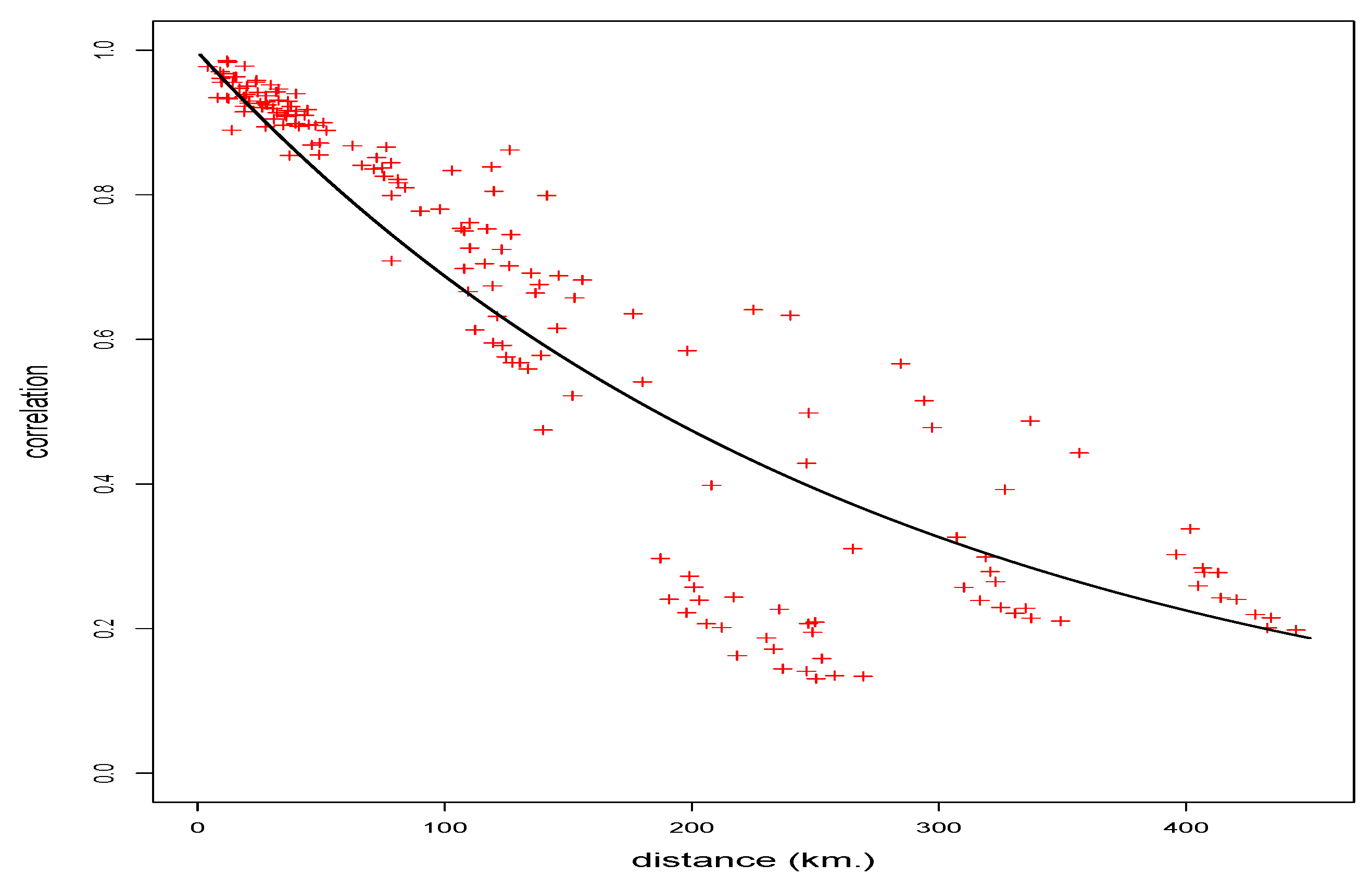
The parameters estimated by WLS for the Alberta wind farm data are and . The data and the fitted pure spatial correlation function are plotted in Figure 5.
3.1.2. Pure Temporal Correlation Function
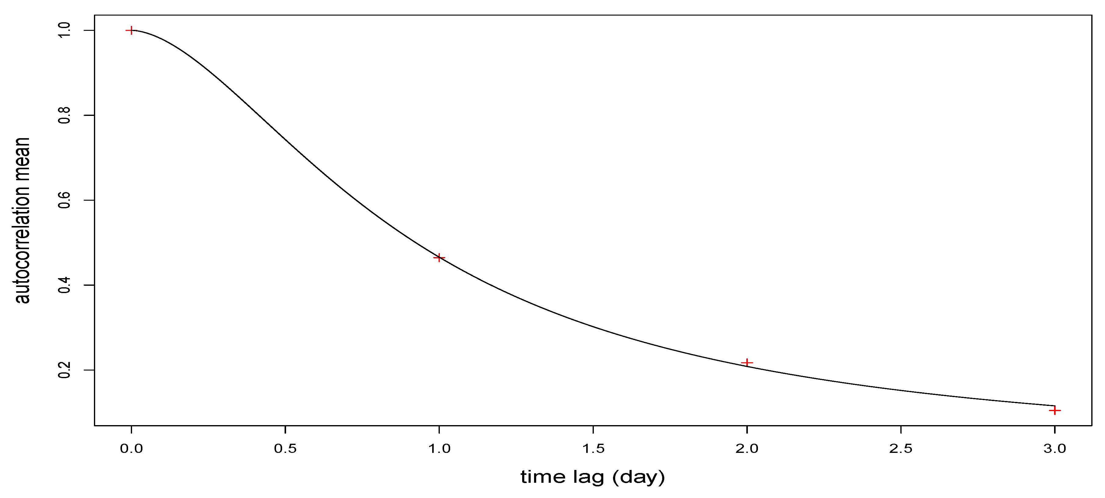
To build the temporal correlation function, we compute the empirical auto-correlations at time lag days for each wind farm and take an average. The Cauchy version of the temporal correlation function that we use is specified as
where the two parameters are estimated as and . The fitted pure temporal correlation function from Equation (5) is drawn with the means of auto-correlation at time lag days in Figure 6.
Then, the separable correlation function is
3.2. Fully Symmetric Model
To relax the separability assumption, we consider a fully symmetric model which introduces the interaction parameter , where is the separable model in Formula (6):
In order to estimate the parameters in this model, we need the cross-correlation between each pair of wind farms at time lag days during the training period.
The estimated , and the difference between the separable and fully symmetric correlation function estimates is insignificant. This result indicates that the separability assumption is satisfied and the interaction component is not necessary in our model. The empirical correlation with the fitted correlation function at time lag , and 4 days is plotted in Figure 7. There is no need for time lags greater than three days, because at days, the cross-correlations are approximately zero for all separations.
3.3. General Stationary Model
Figure 8 shows that the differences in correlation, , at time lags , and 3 days are not close to 0, which means that the assumption of full symmetry is violated, most visibly for . Moreover, the two plots in Figure 8 imply that the symmetry is violated in both the west-east direction and the south-north direction. More precisely, for most pairs , such that is to the west of
This is also true for most pairs , such that is to the south of . We assume that the asymmetry is due to the prevailing winds in southern Alberta. To account for the lack of symmetry, we add the prevailing wind influence in the model by using a Lagrangian correlation function
where we take v as a two dimensional vector.
We build a general stationary correlation function by taking a convex combination based on a fully symmetric model and Lagrangian correlation function:
We use the previously found values for the parameters of , and using WLS we obtain the estimates of and v as , km/day, and km/day where the subscript “1” refers to to west-east and “2” to north-south.
The model identifies the prevailing wind direction as southwesterly, which is consistent with the findings of Sherry and Rival [27] on the wind patterns near the Rocky mountains, see Figure 9. Because a large number of wind farms are clustered in this region, it is not surprising that the wind power outputs are influenced by this prevalent wind pattern.
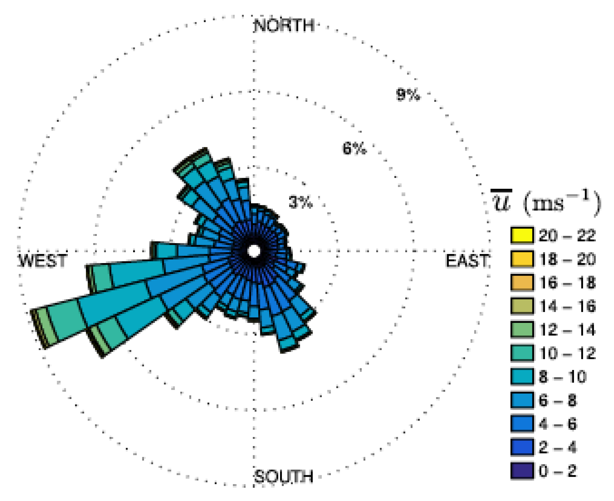
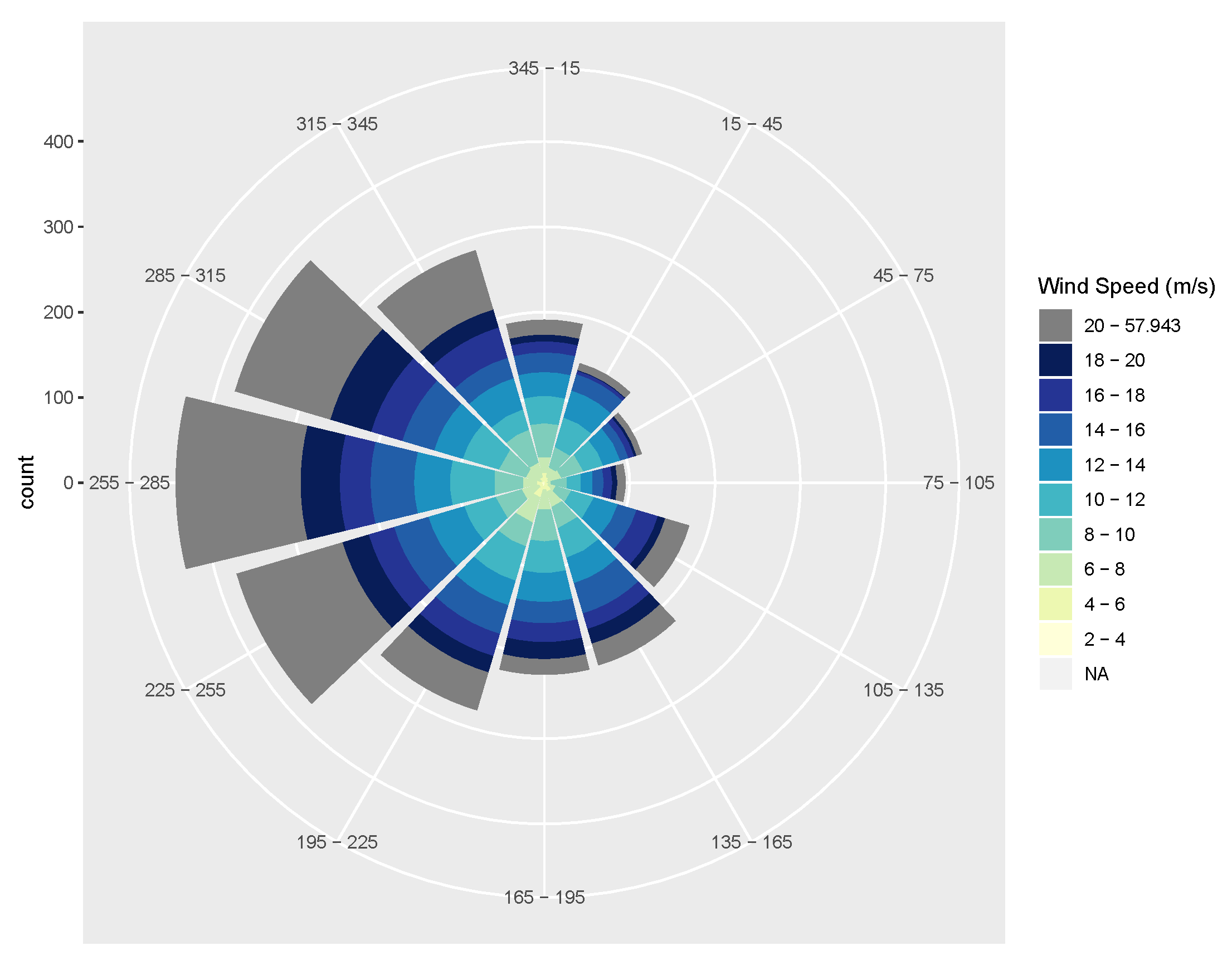
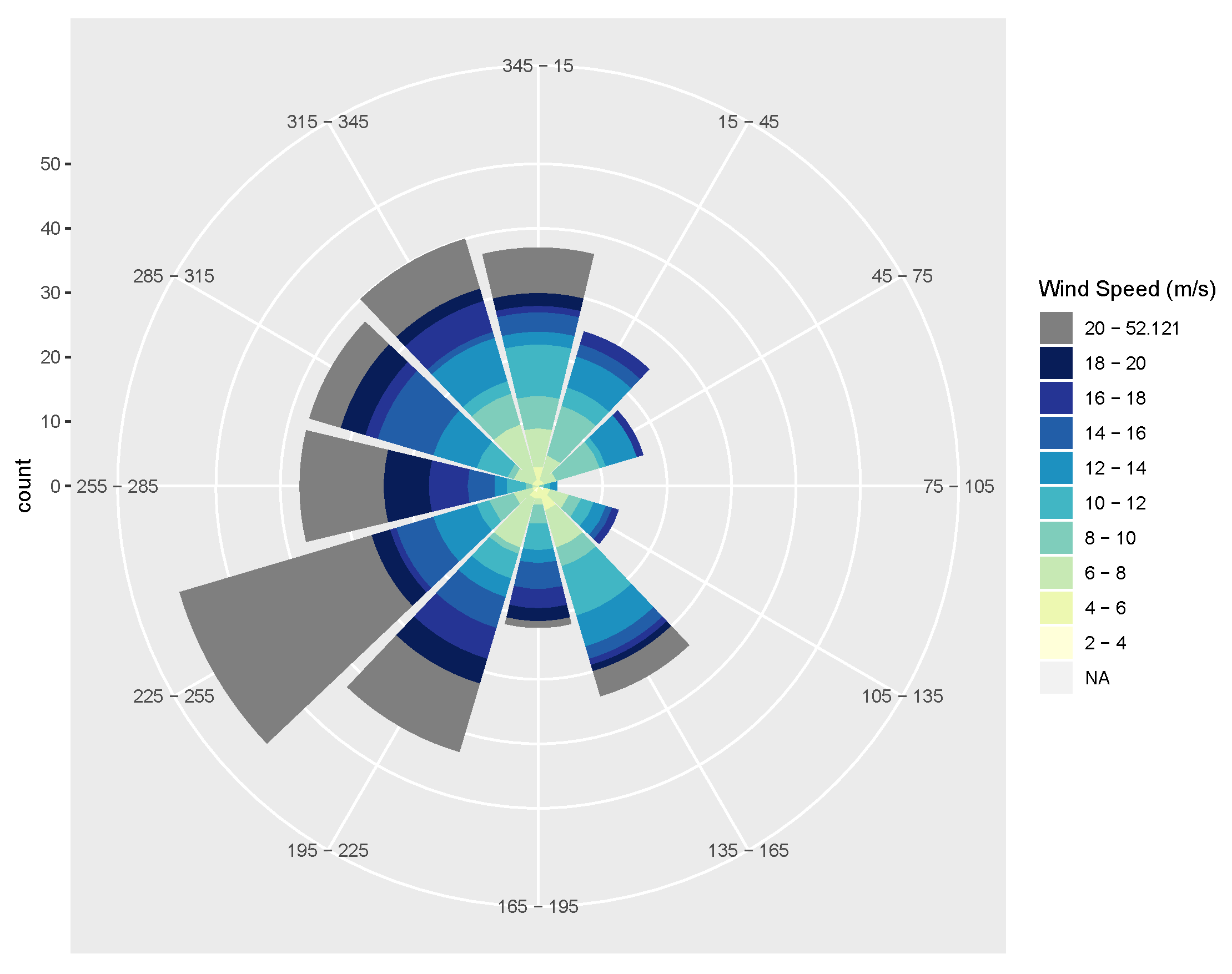
However, the data in Figure 9 were obtained in northern Calgary which is closer to the Rocky Mountains than many of the wind farms and the southwesterly wind may not be prevalent in the entire region that we are considering. To shed light on this, we look at wind speed data pooled from 8 randomly selected weather stations in Alberta, [28]. Figure 10 shows the wind rose plot for this data set. We see that the prevailing wind direction has a westerly component equal to km/day or 1.64 m/s. The southerly component is only km/day, hence is negligible. We note that these are wind speed measurements at 10 m height, whereas Figure 9 shows measurements at 50 m. Fifty meters is a more appropriate height for the majority of wind turbines in Alberta which have towers of around 80 m, hence measurements at this height are likely to be more appropriate than those at 10 m, for forecasting wind power production. In particular, 10 m measurements are subject to random local effects not relevant to wind power. However, there may be a correlation between the two types of measurements. Indeed, we find that the wind patterns from a weather station near wind farms 5 and 10, at Vauxhal, AB gives a wind rose, Figure 11, similar to in Figure 9, in that the prevailing wind direction is southwesterly.
Since the three wind roses indicate a significant westerly component to the prevailing wind direction over the entire region, we also consider a Lagrangian covariance function where the wind direction is assumed to be westerly:
where we take , the subscript “w” indicates a westerly value, as a scalar.
The previous estimates of the parameters of are kept. The estimates of and are and km/day, respectively.
4. Comparison of the Models
We now assess the performance of the three models:
- Model 1with
- Model 2withand km/day and as in Model 1;
- Model 3withand km/day and as in Model 1.
4.1. Goodness of Fit
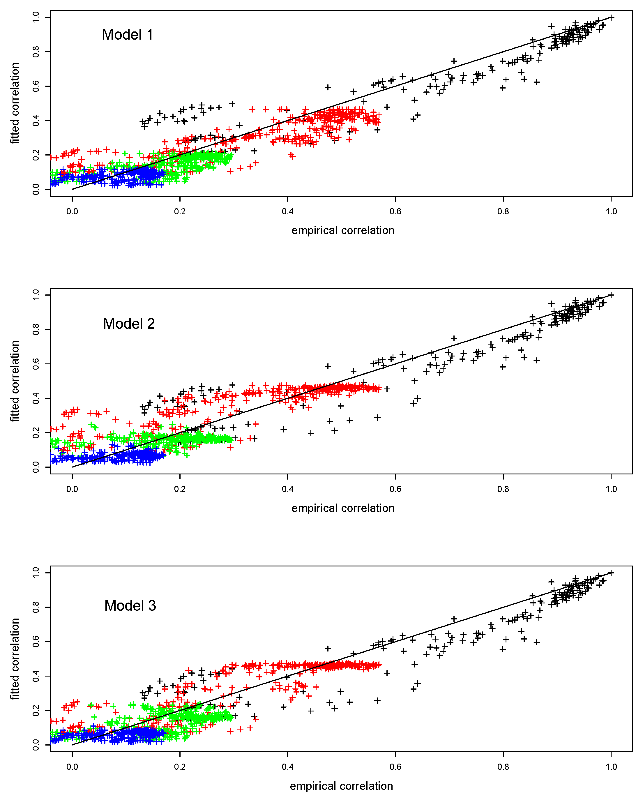
In this section, we compare the goodness of fit of the correlation matrix of each model to the empirical correlations in Figure 12. The three models are very similar for the black and blue points showing the cross correlations at time lags 0 and 3. However, there are some differences in the green and red points, the cross correlations at time lags 1 and 2. There is a larger cluster of red and green points near the line for Model 2, and also the distribution of these points are more symmetrical relative to the line for Model 2 as compared to the other two models. We conclude that Model 2 gives the best fit to the empirical covariances.
4.2. Kriging Predictions
Kriging is a common tool for prediction in the second order modeling framework. The goal is to build a linear estimator of a component of from the observations of some other components . Kriging can also be used as a model evaluation tool as in [5]. The goal is to identify the model with the smallest prediction error. The prediction error can be measured in different ways, such as the root mean square error (RMSE) and the MAE as a function of the site. Since both of these measures scale with the variability of observations, we also use
where and , where is the long time mean of . A larger value indicates a better prediction performance. We also construct 95% prediction intervals (PI) as detailed in Appendix A, and calculate the realized percentage of observations falling outside the 95% PI (POPI). Ideally, this percentage should be close to 5%: a value higher than this indicates that the model is less reliable than it should be, and a lower value indicates that the model is more conservative than it should be.
We focus on two prediction scenarios. In scenario 1, we predict the power output of a given wind farm on a given day based on the observations from all the wind farms (including the same farm) in the past three days. For this scenario, we reproduce the procedure of [5] and compare the three covariance models and the empirical covariance with respect to MSE, RMSE, , and POPI. In scenario 2, we predict the wind power in a given wind farm on a given day based on the observations of all the other wind farms in the past three days. Moreover, the prediction for each farm is based on the parameters estimated by removing all the historical information of the particular farm in the training data. This scenario is important because the selected farm can be viewed as a future site, hence we get an evaluation of the performance of the models in their ability to predict the wind power in future sites.
4.3. Scenario 1: Prediction for an Existing Wind Farm
To forecast the future output of an existing wind farm, we suppose that the historical data for all 19 wind farms are available and the formula of kriging (see e.g., Gaeton and Guyon [29]) for the point prediction at time t, is specified as:
where C is the estimated covariance matrix of . is the cross covariance matrix of with . indicates the transpose of the matrix . is the vector of observations of . We obtain predictions of every day in 2017 for every wind farm using three models given in Formulas (13)–(15). In addition, we make kriging predictions using the empirical covariance matrix of and to provide a baseline case.
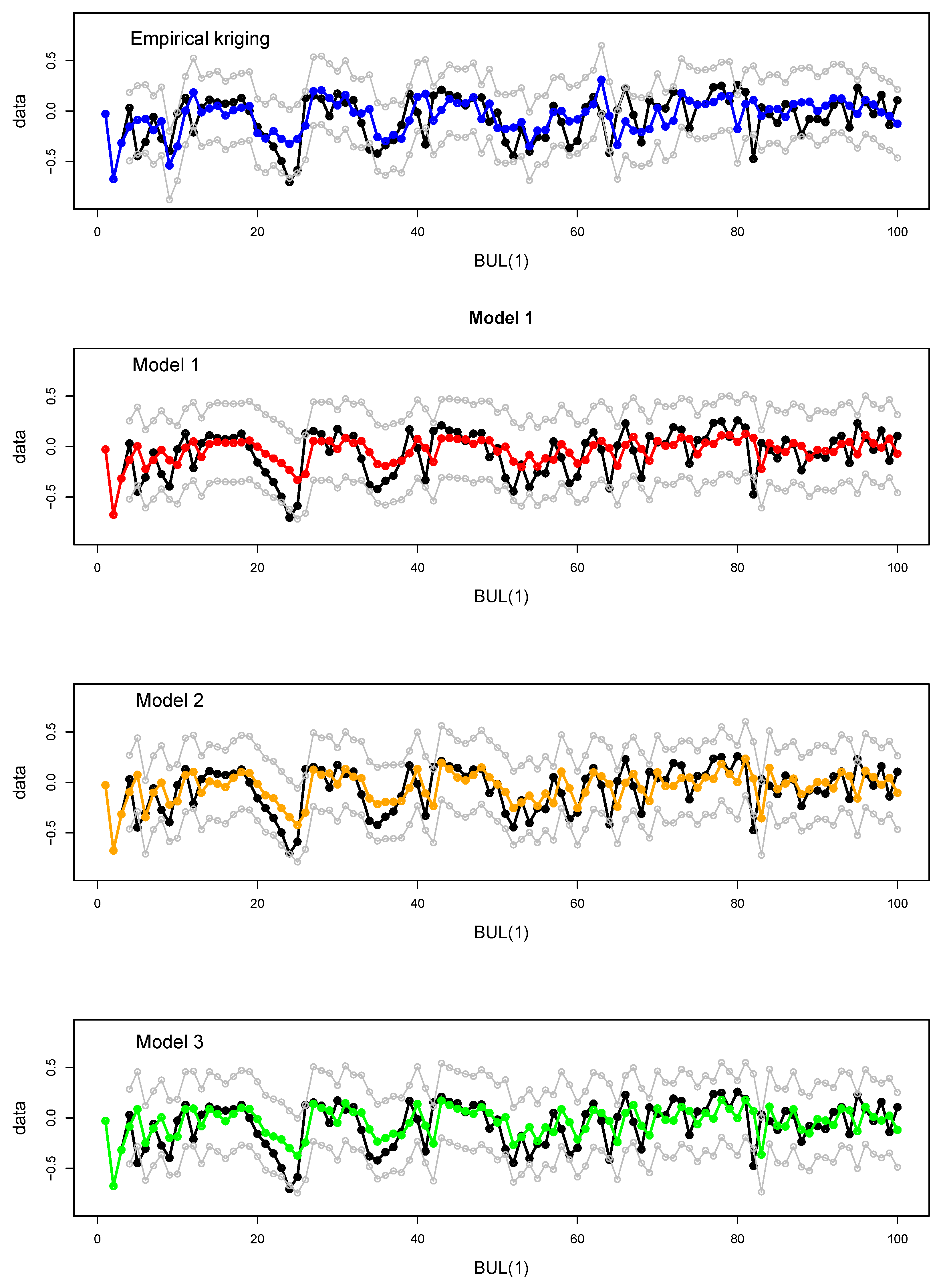
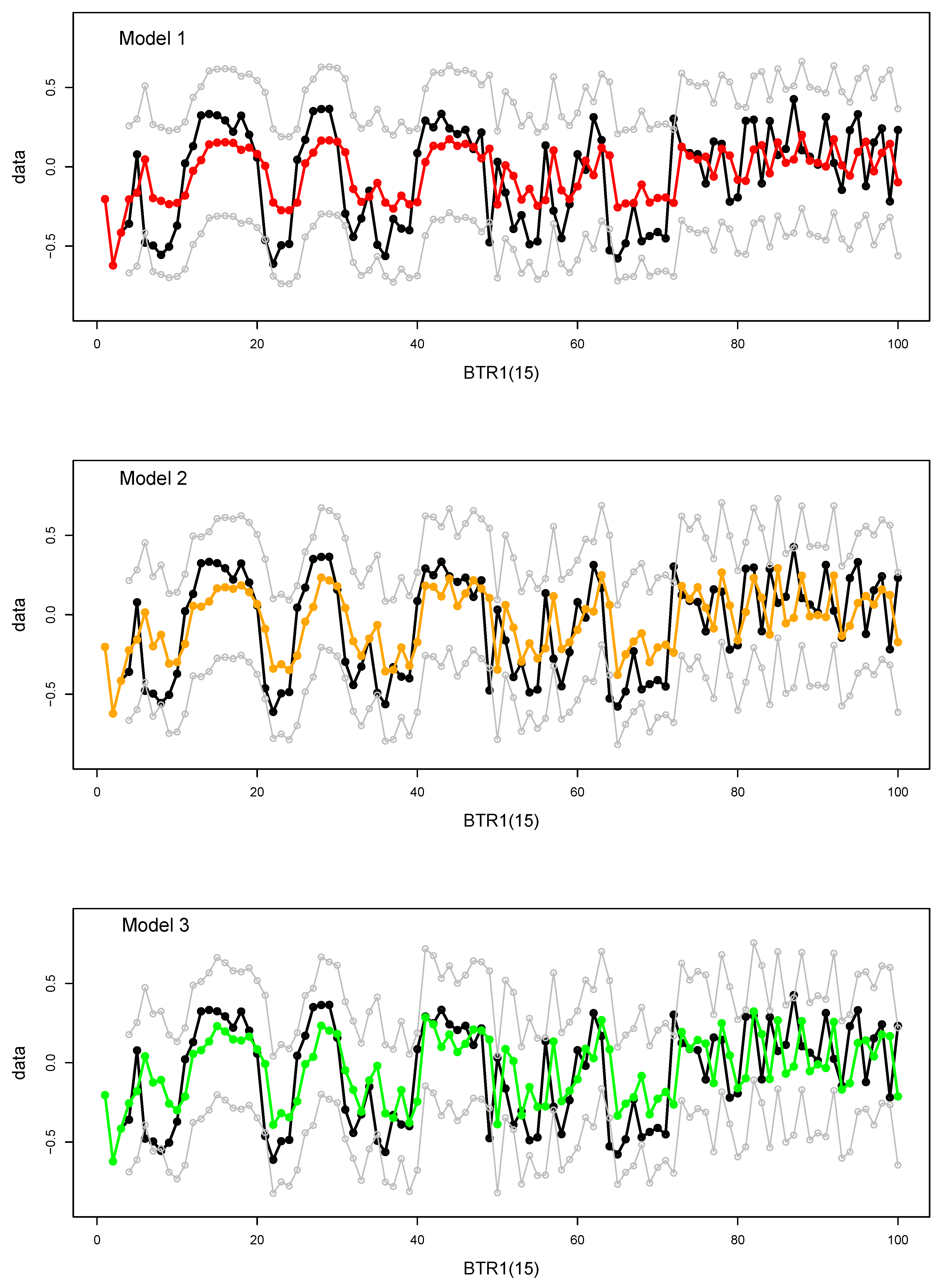
The predicted versus actual power for the first 100 days of 2017 for two farms (BUL and BTR1) are shown in Figure 13 and Figure 14, respectively. These two farms were chosen because BUL is well away from the Rocky Mountains and there are no other wind farms nearby. On the other hand, BTR1 is located close to many other farms near the Rocky Mountains. We expect our predictions to be better for BTR1 than BUL which is confirmed in Figure 13 and Figure 14. Models 1, 2, and 3 perform better than the empirical kriging. Moreover, for both farms, the performance of Model 2 is noticeably better than the others.
For all farms, the mean prediction errors are given in Table 2. On average, Model 2 performs the best in terms of RMSE and MAE, but not , although the difference between Model 1 and Model 2 is small. In POPI, we see that both Models 1 and 2 are performing very close to 5%, whereas Model 1 is more conservative than Model 2.
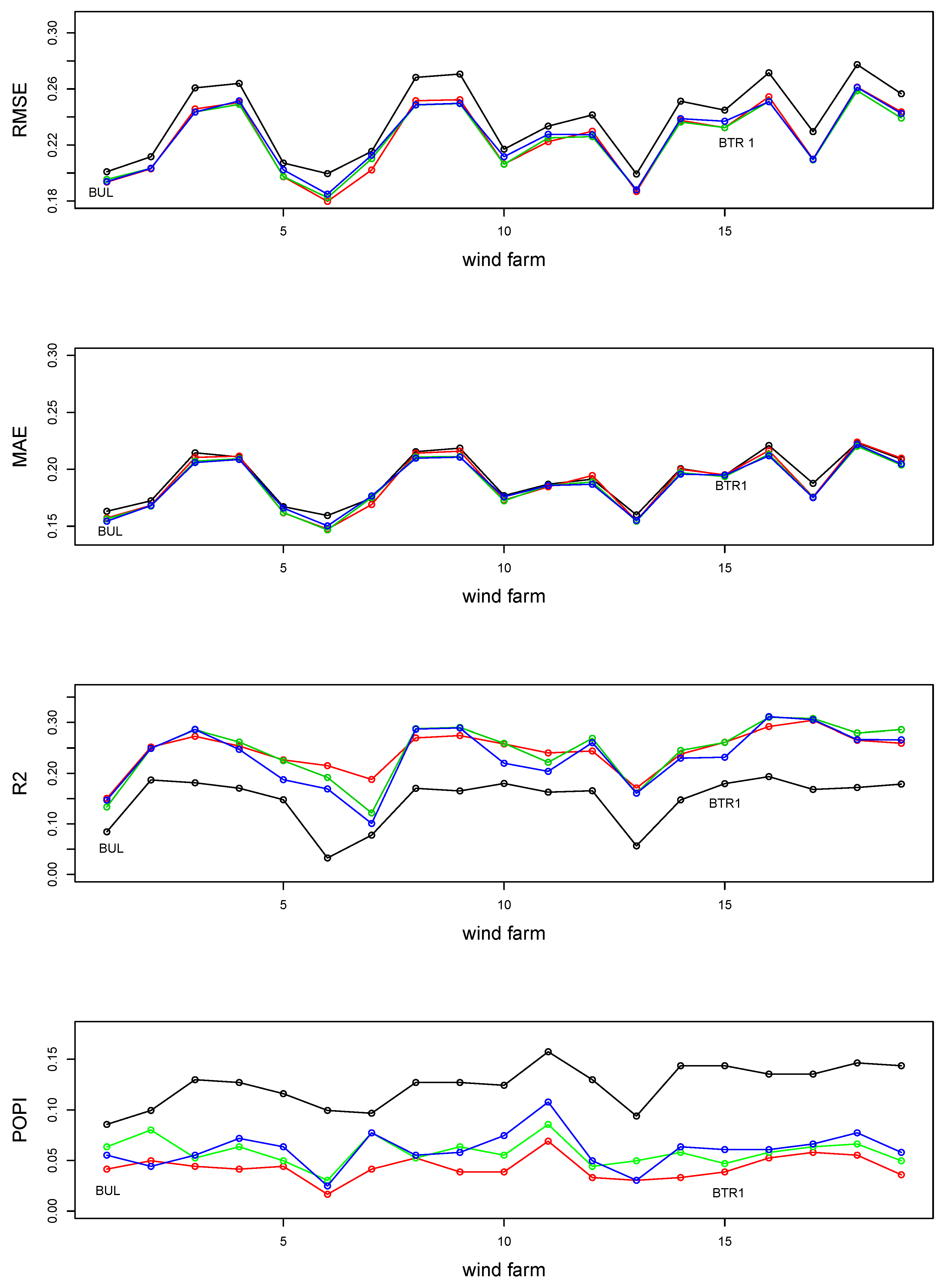
Figure 15 shows RMSE, MAE, , and POPI values for the four models for the farms identified by the number in Figure 1 and Table 1. In these plots, we observe that Model 2 performs consistently better than Model 3 with the exception of BUL for which Model 3 is the best out of three models. Model 2 also performs better than Model 1 for most sites except sites for 6, 7, and 11 for which Model 1 is the best. Overall, we see a pattern that Model 2 performs better on average for sites left of the slanted line in Figure 1 than the sites to the right of the slanted line. It is also interesting to observe that the predictive power of all the models is higher in the region close to the Rocky Mountains, as measured by . This is intuitively correct because there are more farms clustered near the mountains, and the information obtained from nearby farms increases the prediction accuracy for these farms.
After combining all our observations, we conclude that Model 2 is the best model overall.
4.4. Prediction for a New Wind Farm
We select a wind farm to be treated as a new site and perform the estimation procedure by removing all its historical data, and then compare the estimated parameters with the parameters estimated from the actual historical data. For Model 2, we treat the the prevalent wind direction as 242 degrees (measured clockwise, origin north)—the calibrated value of the wind direction for Model 2 using the entire training set—but recalibrate the wind speed and the coefficient of the Lagrangian function with the data of the “new” site removed. Note that we cannot use empirical kriging any more. Thus, we need to re-estimate the parameters in correlation models and acquire 19 sets of values for the parameters in total, where in each iteration we treat a different farm site as the new site. We find that the parameter is zero in all iterations. Thus, we only consider Models 1, 2, and 3.
For each iteration, we predict the observation at the selected site on a given day using the past three days of data for all other sites. Since we are treating the given site as a new site, we do not use observations from that location, so the vector does not include the cross-covariance of the location itself at any time lag, and the dimension of variance-covariance matrix is decreased to . In addition, the modified does not have the historical data from this location.
We give a snapshot of the kriging performances during the first 100 days for sites BUL and BTR1 based on models 1, 2, and 3 in Figure 16 and Figure 17). The prediction accuracy of all three models is very close to that for the existing sites, showing that the models work as effectively for new sites as the existing ones. As in scenario 1, for BUL, it is hard to differentiate the three models, whereas for BTR1, Model 2 performs better than the other two models. In terms of mean prediction errors (Table 3), Models 1 and 2 have similar RMSE and , and both are better than Model 3, while with respect to MAE, Model 2 is the best followed by Model 3. Additionally, POPI for Model 2 is the desirable 5%, whereas Model 1 is less than 4% and Model 3 is more than 6%. Finally, in Figure 18, we see the prediction errors of the models as a function of the farm site. Model 2 is still more accurate for farms close to the mountains, but it does worse (most noticeably in ) for farms sites above the slanted line.
Combining all these observations, we conclude that Model 2 is also the best model for predictions for a new site.
5. The Aggregate Wind Power Generation and the Effect of New Farms
Let represent the wind power output at location x and time t, normalized by the maximum capacity at location x. We apply the same transformations used in preprocessing our data to to arrive at a Gaussian process . More precisely,
or equivalenty,
where is a second order stationary Gaussian process with mean 0, variance and correlation function . is the vector of locations of current wind farms with corresponding maximum capacities . We also consider p new wind farms with locations and capacities . Let be a time point in the future, then is a constant in this case. Thus, the aggregate wind power generation at time is
When are fixed, and are constant. In Appendix B, we derive the formula for the mean of :
Variance of the Aggregate Wind Power Generation
We apply these formulas to find the mean and variance of the aggregate daily average power production of Alberta. Table 4 lists the coordinates and capacities of the new sites that are planned to be built in Alberta. For the new farms, we take as given by Formula (2). Furthermore, the estimated values for the existing farms range between and with a mean value close to 0. Because values do not exhibit a geographical pattern similar to , we take values as 0 for the new farms. It would be interesting to study the relationship of with farm specific factors, such as technology, wind turbine types, etc., which may be used to obtain more accurate estimates of for the new farms; however, this is beyond the scope of the current work. In the estimates below, we take , corresponding to the first day of the year.
Table 5 gives the mean and the variance of the future and current aggregate daily power production. The future production includes the new sites in Table 4 whereas the current production is based on the existing sites listed in Table 1 and Figure 1. We find that with the new wind farms the total power generation will increase by 40.8%, whereas the variability as measured by the standard deviation, of the aggregate generation will increase by 31.5%.
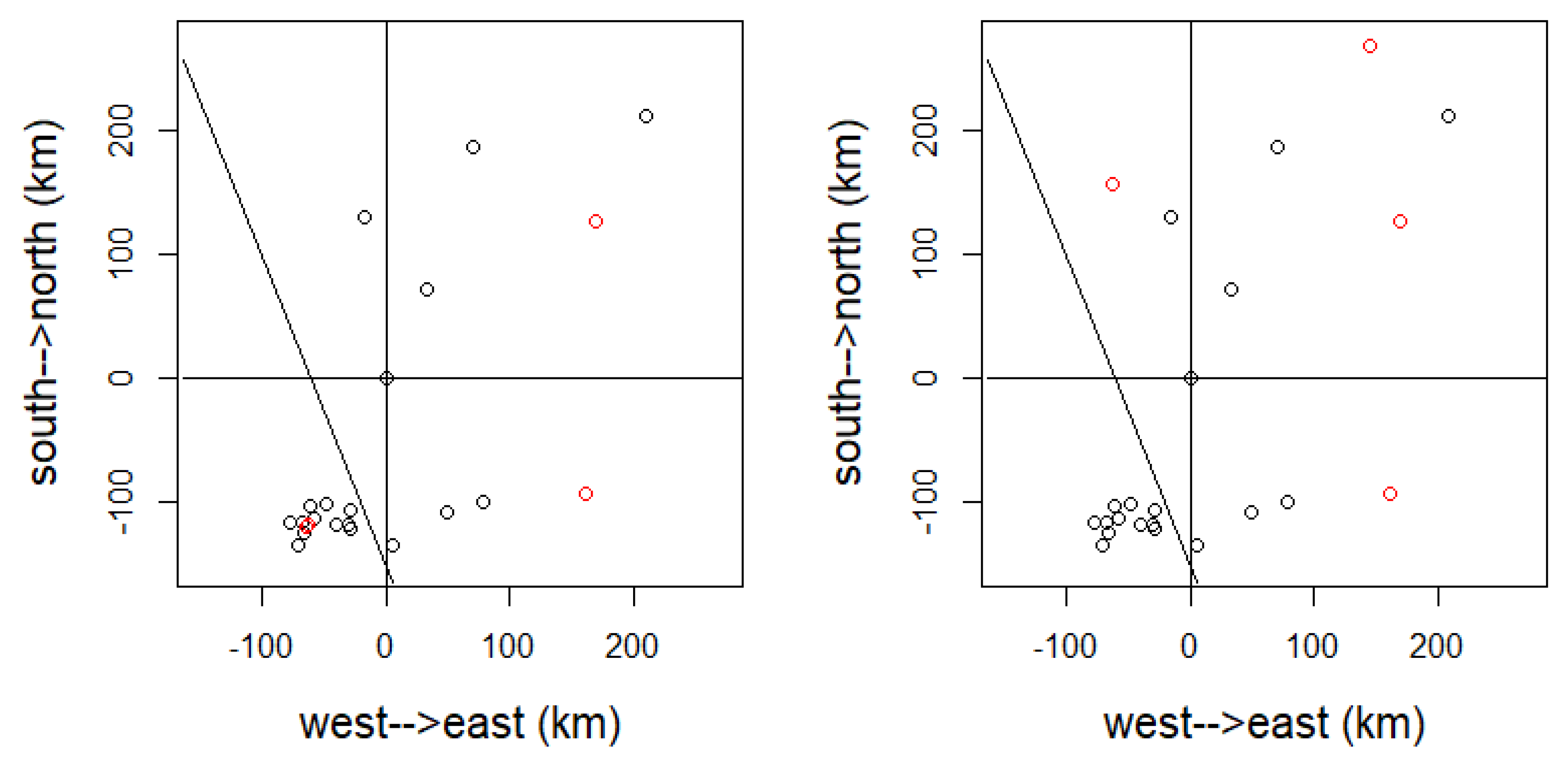
If wind farm power output is independent of the other farms, and if the farms have equal capacity and equal variability in their power generation, a 40.8% increase in the total capacity shown in Table 5 would cause only a increase in the standard deviation of the aggregate power generation. On the other hand, if all the power was generated by single farm and its capacity increased by 40.8%, the standard deviation of its power would also increase by 40.8%. The increase in the standard deviation of the aggregate power in Table 5 is between these two extreme values, indicating that the system will benefit from geographic dispersion; however, there is still room for improvement in terms of reducing the variability of the system. Indeed, a closer look at the locations of the new farms reveals that two of the new sites, Riverview and CRR2, are in the Pincher Creek cluster, see Figure 19, the left panel. For comparison, we consider a hypothetical scenario where we relocate these two sites to new locations to increase geographic dispersion as in Figure 19, the right panel. In this hypothetical scenario, we find that the mean wind power generation would increase by 40.4%, whereas the variability of the wind power generation would increase by 25.47%. This suggests that a reduction in the variability of the aggregate power can be achieved with almost no loss in the mean aggregate power. In the Alberta system, the owners of the new wind farms should also benefit from the reduction in variability.
6. Conclusions and Future Work
Many authorities, including the Alberta government, desire to increase the penetration of renewable energy such as wind power. A reliable forecast of a single wind farm in any particular site and the aggregate wind power in the whole area are helpful to achieve this goal in an efficient and cost-effective manner. In addition, the variability of aggregate wind power and the siting of new wind farms are issues that will be increasingly important as the penetration of renewable energy increases. It is possible to consider wind power output as a second order stochastic process with spatial and temporal dimensions. The most important and difficult step is finding a suitable covariance function for the process. This covariance function not only can describe the correlation in space and time, but also can capture the impact of the atmospheric factors such as the wind speed and direction.
In this study, we assume the transformed daily wind power generation in Alberta is a second-order stationary Gaussian process and estimate several correlation function models proposed by [5]. First, we estimate the simplest correlation function called the separable correlation function. Next, we estimate the space–time interaction parameter in a non-separable but fully symmetric correlation model and find that the space–time interaction is insignificant. With the evidence of asymmetry in our data, we use the Lagrangian correlation function to capture the impact of the prevailing wind. A more complicated asymmetric stationary correlation function is obtained by combining the Lagrangian correlation function with a fully symmetric correlation function. Comparing the goodness of fit for estimations of different models, we observe that the more complicated models fit the data better, that is, the general stationary correlation function model with two parametric partial winds (Model 2) fits the empirical correlations best, and gives the best predictions of the power output of the existing farms.
We use Model 2 to formulate the mean and the variance of the aggregate wind power generation of all wind farms in Alberta. We apply the formulas to calculate the mean of the variance of the aggregate wind power generation including information of the planned new wind farm sites. We find that with the new wind farms, the mean wind power generation will increase by 40.8%, whereas the variability of the wind power generation will increase by 31.5%. Hypothetically, placing the four projected farms away from the clustered region near the Rocky Mountains shows a small decrease in aggregate power output but a significant decrease in its variability.
There are a few challenges which need to be addressed in future work. Gaussian processes are simple and widely used for spatio-temporal data; however, the data of the wind power generation in Alberta is not well suited for the Gaussian assumption. As a result, we have to convert hourly data to daily average data. In our future work, a non-Gaussian spatial-temporal process, such as a hierarchical model, e.g., Bannerjee et al. [30], will be considered to model data with higher time resolution such as hourly or 15-minute data. In addition, Alberta is a large enough region which experiences different prevailing wind speeds and directions. Furthermore, if prevailing wind patterns have a stochastic nature, they may be better captured as stochastic processes (as regime switching processes) but not constants or single-valued parameters, which can also be incorporated in a hierarchical framework.
Author Contributions
This project was the MSc project of Y.L. under the supervision of the D.S., M.W. completed the data analysis. D.W. and H.Z. provided high level guidance on wind energy technology and its development in Alberta. The paper was jointly written by all authors.
Funding
Deniz Sezer is supported by a discovery grant from the Natural Sciences and Engineering Research Council of Canada. DHW’s contribution was supported by the Schulich endowment to the Schulich School of Engineering.
Conflicts of Interest
The authors declare no conflict of interest.
Abbreviations
The following abbreviations are used in this manuscript:
| AESO | Alberta Electric System Operator |
| Cov(X,Y) | Covariance of the random variables X and Y |
| Cor(X,Y) | Correlation of the random variables X and Y |
| Expectation of the random variable X | |
| LOWESS | Locally Weighted Scatterplot Smoothing |
| MAE | Mean Absolute Error |
| MSE | Mean Square Error |
| k-dimensional normal distribution with mean vector and covariance matrix | |
| PI | Prediction Interval |
| POPI | Percent of Observations out of Prediction Intervals |
| RMSE | Root mean Square Error |
| Coefficient of Determination | |
| Var(X) | Variance of the random variable X |
| WLS | Weighted least Squares |
Appendix A. The Prediction Interval
By assumption,
where is the estimated covariance matrix of . We note that there are in total four time lags for each farm, hence the dimension of the vector is . The conditional distribution of given known value for is a multivariate normal , where
We then use the diagonal elements of to construct the prediction intervals for the new predicted values . The prediction interval for i-th wind farm predicted at time t is
where is the i-th element of vector and is the i-th diagonal element of .
Appendix B. Mean and Variance of the Aggregate Wind Power
The expression for is
The covariance, , is given by
It is straightforward to obtain
However, calculating is more complicated. Since t, and are fixed and letting ,
We note that and have a bivariate normal distribution with mean and variance-covariance matrix
Thus, the moment generating function of Y at is
We have
Similarly, we can obtain . Then,
Thus,
References
- Canadian Wind Energy Association. Wind Energy in Alberta. 2018. Available online: http://xxx.lanl.gov/abs/https://canwea.ca/wind-energy/alberta/ (accessed on 1 January 2019).
- Jurasz, J.; Beluco, A.; Canales, F.A. The impact of complementarity on power supply reliability of small scale hybrid energy systems. Energy 2018, 161, 737–743. [Google Scholar] [CrossRef]
- de Oliveira Costa Souza Rosa, C.; Costa, K.A.; da Silva Christo, E.; Bertahone, P.B. Complementarity of Hydro, Photovoltaic, and Wind Power in Rio de Janeiro State. Sustainability 2017, 9, 1130. [Google Scholar] [CrossRef]
- Pinson, P. Wind Energy: Forecasting Challenges for Its Operational Management. Stat. Sci. 2013, 28, 564–585. [Google Scholar] [CrossRef] [Green Version]
- Gneiting, T.; Genton, M.; Guttorp, P. Geostatistical Space-Time Models, Stationarity, Separability and Full Symmetry; Technical Report; Department of Statistics, University of Washington: Seattle, WA, USA, 2006. [Google Scholar]
- Chen, N.; Qian, Z.; Nabney, I.; Meng, X. Wind Power Forecasts Using Gaussian Processes and Numerical Weather Prediction. IEEE Trans. Power Syst. 2014, 29, 656–665. [Google Scholar] [CrossRef]
- Ma, X.; Sun, Y.; Fang, H. Scenario Generation of Wind Power Based on Statistical Uncertainty and Variability. IEEE Trans. Sustain. Energy 2013, 4, 894–904. [Google Scholar] [CrossRef]
- Yang, M.; Lin, Y.; Zhu, S.; Han, X.; Wang, H. Multi-dimensional scenario forecast for generation of multiple wind farms. J. Mod. Power Syst. Clean Energy 2015, 3, 361–370. [Google Scholar] [CrossRef] [Green Version]
- Li, P.; Guan, X.; Wu, J.; Zhou, X. Modeling Dynamic Spatial Correlations of Geographically Distributed Wind Farms and Constructing Ellipsoidal Uncertainty Sets for Optimization-Based Generation Scheduling. IEEE Trans. Sustain. Energy 2015, 6, 1594–1605. [Google Scholar] [CrossRef]
- Gneiting, T.; Larson, K.; Westrick, K.; Genton, M.G.; Aldrich, E. Calibrated Probabilistic Forecasting at the Stateline Wind Energy Center. J. Am. Stat. Assoc. 2006, 101, 968–979. [Google Scholar] [CrossRef]
- Hering, A.S.; Genton, M.G. Powering up with Space-Time Wind Forecasting. J. Am. Stat. Assoc. 2010, 105, 92–104. [Google Scholar] [CrossRef]
- Cavalcante, L.; Bessa, R.; Reis, M.; Browell, J. LASSO vector autoregression structures for very short-term wind power forecasting. Wind Energy 2017, 20, 657–675. [Google Scholar] [CrossRef]
- Browell, J.; Drew, D.R.; Philippopoulos, K. Improved very short-term spatio-temporal wind forecasting using atmospheric regimes. Wind Energy 2018, 21, 968–979. [Google Scholar] [CrossRef]
- Damousis, I.; Alexiadis, M.C.; Theocharis, J.; Dokopoulos, P. A Fuzzy Model for Wind Speed Prediction and Power Generation in Wind Parks Using Spatial Correlation. IEEE Trans. Energy Convers. 2004, 19, 352–361. [Google Scholar] [CrossRef]
- Morales, J.; Minguez, R.; Conejo, A. A methodology to generate statistically dependent wind speed scenarios. Appl. Energy 2010, 87, 843–855. [Google Scholar] [CrossRef]
- Malvaldi, A.; Weiss, S.; Infield, D.; Browell, J.; Leahy, P.; Foley, A.M. A spatial and temporal correlation analysis of aggregate wind power in an ideally interconnected Europe. Wind Energy 2017, 20, 1315–1329. [Google Scholar] [CrossRef] [Green Version]
- Gneiting, T. Nonseparable, Stationary Covariance Functions for Space-Time Data. J. Am. Stat. Assoc. 2002, 97, 590–600. [Google Scholar] [CrossRef]
- Ezzat, A.; Jun, M.; Ding, Y. Spatio-temporal asymmetry of local wind fields and its impact on short-term wind forecasting. IEEE Trans. Sustain. Energy 2018, 9, 1437–1447. [Google Scholar] [CrossRef] [PubMed]
- Reichenberg, L.; Wojciechowski, A.; Hedenus, F.; Johnsson, F. Geographic aggregation of wind power—An optimization methodology for avoiding low outputs. Wind Energy 2017, 20, 19–32. [Google Scholar] [CrossRef]
- Tejeda, C.; Gallardo, C.; Domínguez, M.; Gaertner, M.; Gutierrez, C.; Castro, M. Using wind velocity estimated from a reanalysis to minimize the variability of aggregated wind farm production over Europe. Wind Energy 2018, 21, 174–183. [Google Scholar] [CrossRef]
- MacCormack, J.; Westwick, D.; Zareipour, H.; Rosehart, W. Stochastic modeling of future wind generation scenarios. In Proceedings of the 2008 40th North American Power Symposium, Calgary, AB, Canada, 28–30 September 2008; pp. 1–7. [Google Scholar] [CrossRef]
- Miettinen, J.; Holttinen, H. Characteristics of day-ahead wind power forecast errors in Nordic countries and benefits of aggregation. Wind Energy 2016, 20, 959–972. [Google Scholar] [CrossRef]
- Baxevani, A.; Lennartsson, J. A spatiotemporal precipitation generator based on a censored latent Gaussian field. Water Resour. Res. 2015, 51, 4338–4358. [Google Scholar] [CrossRef] [Green Version]
- Glasbey, C.; Nevison, I.; Hunter, A. Parameter Estimators for Gaussian Models with Censored Time Series and Spatio-temporal Data. In COMPSTAT98: Proceedings in Computational Statistics; Payne, R., Green, P., Eds.; Physica-Verlag: Heidelberg, Germany, 1998; pp. 323–328. [Google Scholar]
- Allcroft, D.J.; Glasbey, C.A. A latent Gaussian Markov random-field model for spatiotemporal rainfall disaggregation. J. R. Stat. Soc. Ser. C Appl. Stat. 2003, 52, 487–498. [Google Scholar] [CrossRef]
- Cleveland, W.S. Robust Locally Weighted Regression and Smoothing Scatterplots. J. Am. Stat. Assoc. 1979, 74, 829–836. [Google Scholar] [CrossRef]
- Sherry, M.; Rival, D. Meteorological phenomena associated with wind-power ramps downwind of mountainous terrain. J. Renew. Sustain. Energy 2015, 7. [Google Scholar] [CrossRef]
- Alberta Agriculture and Forestry. Current and Historical Alberta Weather Station Data Viewer. Available online: https://agriculture.alberta.ca/acis/alberta-weather-data-viewer.jsp (accessed on 4 January 2019).
- Gaeton, C.; Guyon, X. Spatial Statistics and Modeling; Springer Science+Business Media, LLC: Berlin/Heidelberg, Germany, 2010. [Google Scholar]
- Banerjee, S.; Carlin, B.; Gelfand, A. Hierarchical Modeling and Analysis of Spatial Data; CRC Press: Boca Raton, FL, USA, 2015; Chapter 5; pp. 129–175. [Google Scholar]
Figure 1.
Locations of the 19 wind farms in Alberta. North is vertically upwards. The width and height of map are ≈500 kms. The Rocky Mountains start just to the west of wind farm no. 17 and follow the direction of the slanted line to Banff National park. The remainder of the area in the figure is flat.

Figure 2.
Histograms of hourly wind power production in 19 wind farms in the training test. The hourly wind power production values in MW are shown in the x-axis.
Figure 2.
Histograms of hourly wind power production in 19 wind farms in the training test. The hourly wind power production values in MW are shown in the x-axis.

Figure 3.
Histograms of daily wind power production in 19 wind farms after preprocessing in the training set.
Figure 3.
Histograms of daily wind power production in 19 wind farms after preprocessing in the training set.

Figure 4.
The flow chart of data preprocessing.

Figure 5.
Empirical correlations against distance with fitted pure spatial correlation.

Figure 6.
Empirical auto-correlations against time lags with fitted pure temporal correlation.

Figure 7.
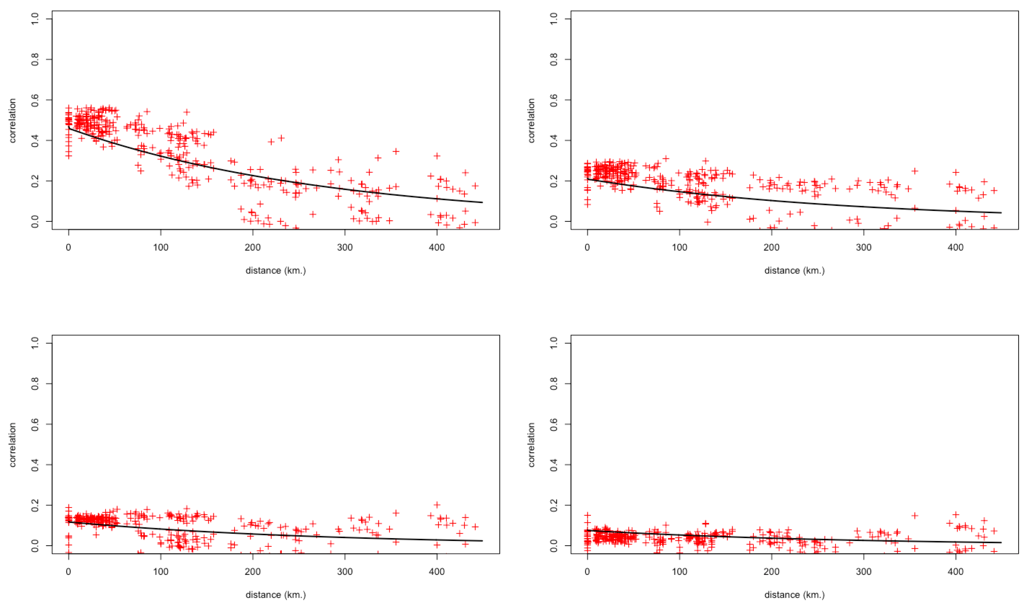
Empirical spatial-temporal correlation plots with fitted correlation function at time lag one day (upper left), two days (upper right), three days (lower left), four days (lower right).
Figure 7.
Empirical spatial-temporal correlation plots with fitted correlation function at time lag one day (upper left), two days (upper right), three days (lower left), four days (lower right).

Figure 8.
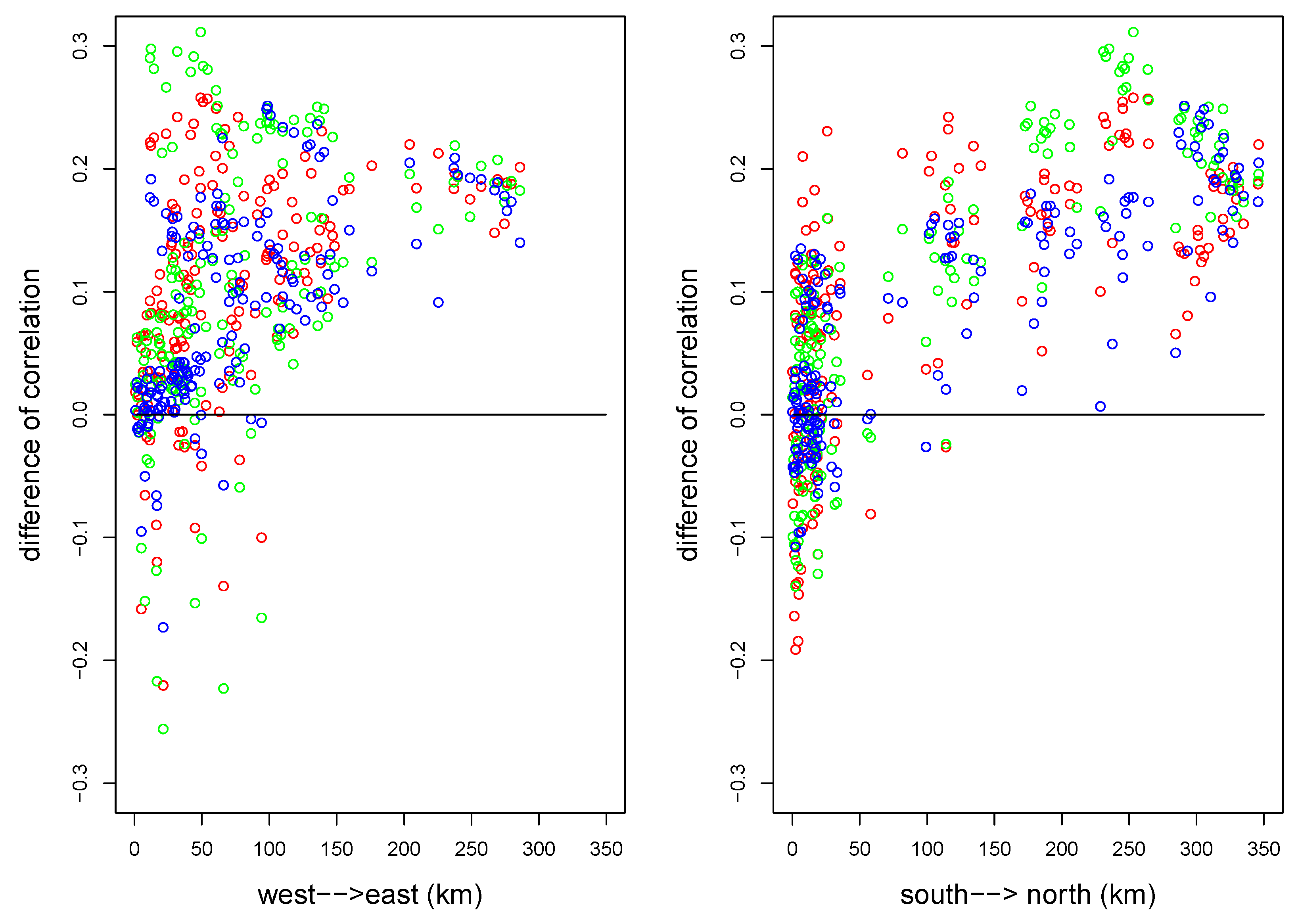
The left plot indicates the difference between the empirical west-to-east and east-to-west cross-correlations for the 171 distinct pairs of wind farms at temporal lags one day (red), two days (green), and three days (blue) against the east-west distance between the farms. The right plot indicates the difference between the empirical south-to-north and north-to-south cross-correlations against the north-south distance between the farms.
Figure 8.
The left plot indicates the difference between the empirical west-to-east and east-to-west cross-correlations for the 171 distinct pairs of wind farms at temporal lags one day (red), two days (green), and three days (blue) against the east-west distance between the farms. The right plot indicates the difference between the empirical south-to-north and north-to-south cross-correlations against the north-south distance between the farms.

Figure 9.
Wind rose plot taken from Sherry and Rival [27]. The measurements were made at a height of 50 m using a wind mast on the northern outskirts of Calgary.
Figure 9.
Wind rose plot taken from Sherry and Rival [27]. The measurements were made at a height of 50 m using a wind mast on the northern outskirts of Calgary.

Figure 10.
Wind rose plot from eight randomly selected weather stations in the region defined in Figure 1.
Figure 10.
Wind rose plot from eight randomly selected weather stations in the region defined in Figure 1.

Figure 11.
Wind rose from the weather station at Vauxhall, AB, midway between farms 5 and 10.

Figure 12.
Goodness of fit of the three models: black, red, green, and blue colors correspond to cross correlations of any two locations at time lags 0, 1, 2, and 3 days, respectively.
Figure 12.
Goodness of fit of the three models: black, red, green, and blue colors correspond to cross correlations of any two locations at time lags 0, 1, 2, and 3 days, respectively.

Figure 13.
Actual daily power production (black) versus predicted values when BUL is treated as an existing wind farm. The x-axis is in days. Prediction intervals are in color gray.
Figure 13.
Actual daily power production (black) versus predicted values when BUL is treated as an existing wind farm. The x-axis is in days. Prediction intervals are in color gray.

Figure 14.
Actual daily power production (black) versus predicted values when CR1 is treated as an existing wind farm. The x-axis is in days. Prediction intervals are in color gray.
Figure 14.
Actual daily power production (black) versus predicted values when CR1 is treated as an existing wind farm. The x-axis is in days. Prediction intervals are in color gray.

Figure 15.
Root mean square error (RMSE), mean absolute error (MAE), coefficient of determination (), and percent of observations out of prediction intervals (POPI) for predicting power output from all wind farms. Empirical: red. Model 1: red. Model 2: green. Model 3: blue.
Figure 15.
Root mean square error (RMSE), mean absolute error (MAE), coefficient of determination (), and percent of observations out of prediction intervals (POPI) for predicting power output from all wind farms. Empirical: red. Model 1: red. Model 2: green. Model 3: blue.

Figure 16.
Actual daily power production (black) versus predicted values when BUL is treated as a new wind farm. The x-axis is in days. Prediction intervals are in color gray.
Figure 16.
Actual daily power production (black) versus predicted values when BUL is treated as a new wind farm. The x-axis is in days. Prediction intervals are in color gray.

Figure 17.
Actual daily power production (black) versus predicted values when BTR1 is treated as a new wind farm. The x-axis is in days. Prediction intervals are in color gray.
Figure 17.
Actual daily power production (black) versus predicted values when BTR1 is treated as a new wind farm. The x-axis is in days. Prediction intervals are in color gray.

Figure 18.
RMSE, MAE, , and POPI for predicting a new wind farm as a function of the farm site. Model 1: black. Model 2: red. Model 3: green.
Figure 18.
RMSE, MAE, , and POPI for predicting a new wind farm as a function of the farm site. Model 1: black. Model 2: red. Model 3: green.

Figure 19.
The left figure shows the relative locations of the planned sites in Table 4. The right figure shows a hypothetical relocation of the planned sites. The straight lines in the figures are the same as in Figure 1.


Table 1.
Alberta wind farms, their capacity in Megawatts (second row), and specific variances in daily production (third row).
Table 1.
Alberta wind farms, their capacity in Megawatts (second row), and specific variances in daily production (third row).
| BUL | BSR1 | CRR1 | AKE1 | TAB1 | NEP1 | HAL1 | KHW1 | OWF1 | SCR3 |
| 1 | 2 | 3 | 4 | 5 | 6 | 7 | 8 | 9 | 10 |
| 29 | 300 | 77 | 73 | 81 | 82 | 150 | 63 | 46 | 30 |
| 0.046 | 0.055 | 0.072 | 0.074 | 0.048 | 0.041 | 0.048 | 0.079 | 0.084 | 0.053 |
| SCR2 | GWW1 | SCR4 | ARD1 | BTR1 | CR1 | CRE3 | IEW1 | IEW2 | |
| 11 | 12 | 13 | 14 | 15 | 16 | 17 | 18 | 19 | |
| 30 | 71 | 88 | 68 | 66 | 39 | 20 | 66 | 66 | |
| 0.053 | 0.064 | 0.042 | 0.067 | 0.066 | 0.08 | 0.055 | 0.082 | 0.072 |
Table 2.
Mean prediction errors for all wind farms.
| Model | ||||
|---|---|---|---|---|
| Empirical | 0.2379 | 0.1920 | 0.1484 | 0.1234 |
| Model 1 | 0.2242 | 0.1886 | 0.2440 | 0.0429 |
| Model 2 | 0.2238 | 0.1869 | 0.2446 | 0.0584 |
| Model 3 | 0.2255 | 0.1873 | 0.2326 | 0.0608 |
Table 3.
Mean prediction errors for a new wind farm.
| Model | ||||
|---|---|---|---|---|
| Model 1 | 0.2245 | 0.1892 | 0.2432 | 0.0366 |
| Model 2 | 0.2246 | 0.1878 | 0.2397 | 0.0538 |
| Model 3 | 0.2260 | 0.1880 | 0.2306 | 0.0621 |
Table 4.
Future wind farms.
| Sites | Capacity (MW) | Coordinates |
|---|---|---|
| Sharp Hills, Oyen | 248.4 | |
| Riverview, Pincher Creek | 115 | |
| CRR2 Pincher Creek | 30.6 | |
| Whitla Wind, Medicine Hat | 201.6 |
Table 5.
Current and future aggregate daily production.
| Farms | Total Capacity (MW) | Mean Production (MW) | Standard Deviation (MW) |
|---|---|---|---|
| Current (Farms 1–19) | 1445 | 737.23 | 381.34 |
| Future (Farms 1–23) | 2040.6 | 1037.93 | 502.34 |
© 2019 by the authors. Licensee MDPI, Basel, Switzerland. This article is an open access article distributed under the terms and conditions of the Creative Commons Attribution (CC BY) license (http://creativecommons.org/licenses/by/4.0/).
Share and Cite
MDPI and ACS Style
Luo, Y.; Sezer, D.; Wood, D.; Wu, M.; Zareipour, H. Estimation of the Daily Variability of Aggregate Wind Power Generation in Alberta, Canada. Energies 2019, 12, 1998. https://doi.org/10.3390/en12101998
AMA Style
Luo Y, Sezer D, Wood D, Wu M, Zareipour H. Estimation of the Daily Variability of Aggregate Wind Power Generation in Alberta, Canada. Energies. 2019; 12(10):1998. https://doi.org/10.3390/en12101998
Chicago/Turabian StyleLuo, Yilan, Deniz Sezer, David Wood, Mingkuan Wu, and Hamid Zareipour. 2019. "Estimation of the Daily Variability of Aggregate Wind Power Generation in Alberta, Canada" Energies 12, no. 10: 1998. https://doi.org/10.3390/en12101998
Note that from the first issue of 2016, this journal uses article numbers instead of page numbers. See further details here.