Non-Probabilistic Time-Varying Reliability-Based Analysis of Corroded Pipelines Considering the Interaction of Multiple Uncertainty Variables

Abstract

Reliability analysis of corroded pipelines is critical to the integrity and safe working of pipeline infrastructure. Aiming at less probability information is obtained for corrosion pipeline engineering, and the mechanical properties of pipeline with corrosion defects deteriorate caused by the accumulative effect of corrosion growth. Based on the quasi-static analysis method and non-probability theory, this paper presents a reliability model for assessing corroded pipelines with corrosion growth. In fact, reliability analysis of corroded pipelines needs to consider the interaction of multiple uncertainty variables. By introducing interaction theory, a mathematical model of corrosion defects considering the interaction of variables is put forward. Moreover, this paper develops a non-probabilistic time-varying reliability method for pipeline systems with multiple defects. Thus, several numerical examples are investigated to discuss the effectiveness of the proposed methodology. The results show that a two-dimensional or even three-dimensional ellipsoid model with correlation has more accurate results to evaluate corroded pipelines under the interaction of multiple corroded defects with poor information. Furthermore, a non-probabilistic time-varying reliability model is established according to the time-varying characteristics of the corroded pipeline under the influence of multiple factors. An effective complement to the theory of non-probabilistic reliability analysis of system is investigated. The analysis of the results suggests that interaction of corroded pipeline has a negligible impact on reliability. It also provides a theoretical basis for maintenance and is of great significance for risk- and reliability-informed decisions regarding buried oil and gas pipelines.

1. Introduction

Oil and gas have been the main source of energy [1,2]. As a lifeline project, the safety operation of the pipeline plays an important role for energy transportation. Pipelines with corrosion defects introduce risk to the structural safety of the pipeline infrastructure. Corrosion therefore threatens the normal operation of the pipeline, even causing secondary accidents [3,4]. In particular, the interaction of corroded defects can affect each other and cause damage to the pipeline [5,6]. Moreover, analysis of the interaction of multiple corrosion defects provides more accurate and reliable prediction of the safety assessment of pipelines as corroded defects are usually present within a sufficiently close spatial distance [7]. Thus, system reliability analysis is closer to practical engineering. Due to the decay characteristic of corrosion with time, the resistance of the pipeline has the trend of decrease, which is a dynamic time-varying process [8,9].

Reliability analysis methods are useful tools for maintenance optimization of corroded pipelines. With reliability analysis, a lot of research work on the risk and reliability of corroded pipelines has been presented [10,11,12,13,14]. However, reliability analysis of corroded pipelines based on classical probabilistic reliability theory needs a lot of statistical data. In fact, credible probability models may not be suitable if experimental data are insufficient. In addition, it is difficult to obtain accurate probability distribution based on small samples in pipeline engineering, and there is also a high cost involved in collecting data. Ben-Haim and Elishakoff proposed the concept of non-probabilistic set theory in the field of applied mechanics [15,16]. The non-probability set theory convex method proposes that the distribution and assumptions of uncertainty information need not be obtained, since the bounds can be confirmed with small samples. Thus, when there is not enough data to construct the edge probability distribution of variables, non-probabilistic convex sets can be used to describe the uncertainty variables [17]. The convex domain is used to process the uncertainty variables, whose shape and size reflect the degrees of cognition of the variables and the fluctuation range of the uncertainty variable, respectively. The interval model and the ellipsoid model are the most widely used in the field of non-probabilistic reliability. The interval model can only deal with independent variables, while the ellipsoid model can deal with problems involving dependent variables [18,19]. Thus, the modeling method of the ellipsoid convex set model is applied to practical engineering involved interaction research [20].

Assessment of reliability involve a process of dynamic change throughout the life of the project. Based on random process theory considering the influence of time for structural resistance and stress, the methods of first transcendence and of performance extremes substituted for the dynamic reliability method [21,22]. Furthermore, the dynamic reliability method, being based on random process, needs numerous data [23].

In this work a non-probabilistic method is presented to analyze the reliability of pipelines by considering the interaction coefficients in corroded pipelines. More importantly, an interaction model is proposed for analyzing the influence of two-dimensional and three-dimensional uncertainty spatial domains based on the ellipsoidal theory. Specifically, according to convex model theory, the interaction model is used to study the non-probabilistic reliability design of corroded pipelines with the correlation of parameters. Furthermore, a method regarding the interaction degree for multiple correlation influences of corroded pipelines with uncertainty parameters is presented. Combined with the structural decay of resistance and small sample, the non-probabilistic time-varying reliability analysis of corroded pipelines was set up. It is anticipated that this work develops a promising methodology for the safe assessment of the interaction effect between multiple uncertain variables of corroded defects and for system non-probabilistic reliability analysis, as well as supplementing risk decision and reliability analysis of corroded pipeline engineering.

2. Failure Mode of Local Corroded Pipelines

2.1. Pipeline with Local Corrosion

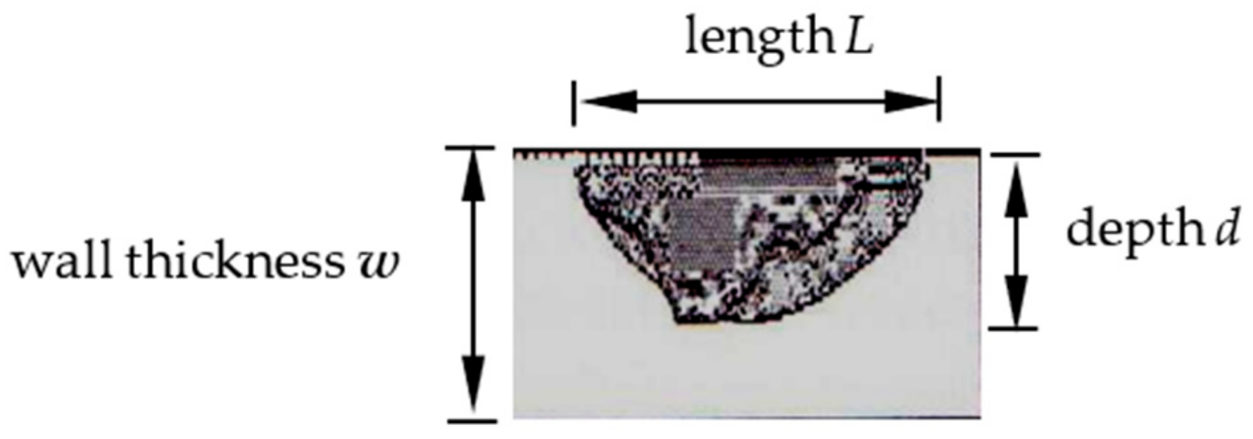
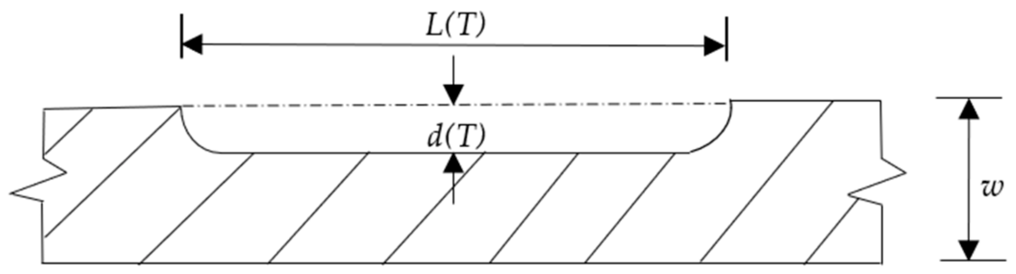
Local corrosion failure of pressure pipelines is one of the main modes. For many corrosion failures of oil and gas pipelines, the proportion of failures caused by local corrosion of pipelines is much larger than that of general corrosion [24]. Figure 1 shows the performance of the local corrosion of the pipeline. The main failure mode of local corrosion of pipelines is local blasting failure, the reason being that the residual wall thickness of local corrosion defects cannot withstand internal pressure. Thus, it not only causes local blasting of pipelines, but also causes a large amount of leakage, with the pipeline pressure also dropping significantly. Most studies suggest simplifying the ideal corrosion defect to equal-depth shapes, as shown in Figure 2.

Many burst pressure prediction models were evaluated by the B31G, modified B31G, RSTRENG, and PCORRC certification programs [25,26]. This paper obtains the ASME B31G standard; the failure pressure of corroded pipeline is given by [27]:

$$P_f=2\left({\sigma }_s+68.95\right)\frac{w}{D}\times \frac{1-0.85d/w}{1-0.85d/\left(w{M}_T\right)},$$

(1)

where ${\sigma }_s$ is the yield strength of material, $w$ is the wall thickness of the pipeline, $d$ is the corroded depth of the defect, $D$ is the diameter of the pipeline, and $M_T$ is the Folias coefficient, which is related to the length of the corroded defect, the outer diameter of the pipeline, and the wall thickness.

When $\frac{L^2}{Dw}\le 50$, the Folias coefficient $M_T$ can be expressed as:

$$M_T=\sqrt{1+0.6275\frac{L^2}{Dw}-0.003375\frac{L^4}{D^2{w}^2}},$$

(2)

where $L$ is the length of the corrosion defect.

When $\frac{L^2}{Dw}>50$, the Folias coefficient $M_T$ can be expressed as:

$$M_T=0.032\left(\frac{L^2}{Dw}\right)+3.3.$$

(3)

2.2. Time-Varying Failure Modes of Pipeline with Local Corrosion

Since most practical engineering does not have accurate data to fit the corrosion growth model, for simplicity, the rate of corrosion growth is a linear process. For the assumption of the quasi-steady state of corrosion not affect the interaction of different studied uncertain variables, the corrosion growth process can be a linear function over time, as follows [28]:

$$d\left(T\right)=d_0+v_d\Delta T,$$

(4)

$$L\left(T\right)=L_0+v_L\Delta T,$$

(5)

$$b\left(T\right)=b_0+v_b\Delta T,$$

(6)

where $d_0$ is the initial corroded depth of defect; $v_d$ is the rate of radial growth, which is given by $v_d=\Delta d/\Delta T$; $L_0$ is the length of initial corroded defect; $v_L$ is the rate of axial growth, which is given by $v_L=\Delta L/\Delta T$; $b_0$; is the width of initial corroded defect; $v_b$ is the rate circumferential growth, which is given by $v_b=\Delta b/\Delta T$; and $\Delta T$ is the time interval.

Based on the corrosion growth characteristics of the pipeline, combined with the formula (1), (4) and (5), the pressure of the time-dependent corroded pipeline model can be obtained:

$$P_f=2\left({\sigma }_s+68.95\right)\frac{w}{D}\times \frac{1-0.85\left(d_0+v_d\Delta T\right)/w}{1-0.85\left(d_0+v_d\Delta T\right)/\left(w{M}_T\right)}.$$

(7)

2.3. Interaction of Corroded Defects

Interaction refers to the degree of closeness between two or more variables. The interaction coefficient measures the degree and direction of the interaction among non-independent random variables. When the interaction coefficient is positive, it means that when one variable increases, the other increases. When the interaction coefficient is negative, it means that one variable increases while the other variable decreases. Therefore, the absolute value of the interaction coefficient indicates the interaction of random variables. Furthermore, the magnitude of the interaction coefficient of random variables and its impact on the probability of failure vary with the practical situation.

Due to the interaction of the uncertainty variables for corroded defects, the interaction coefficient can be obtained from multiple sets of corroded defect data obtained by pipeline detection. Assuming that two sets of random variables are $x_1,x_2,x_3\cdots x_n$ and $y_1,y_2,y_3\cdots y_n$, respectively. The interaction coefficient has the following expression:

$$\rho =\frac{n{\displaystyle \sum _{i=1}^n{x}_i{y}_i}-{\displaystyle \sum _{i=1}^n{x}_i}\cdot {\displaystyle \sum _{i=1}^n{y}_i}}{\sqrt{n{\displaystyle \sum _{i=1}^n{x}_i^2}-{\left({\displaystyle \sum _{i=1}^n{y}_i}\right)}^2}\cdot \sqrt{n{\displaystyle \sum _{i=1}^n{x}_i^2}-{\left({\displaystyle \sum _{i=1}^n{y}_i}\right)}^2}},$$

(8)

where $\rho$ is the interaction coefficient and $x_i$, $y_i$ are the interaction variables.

When $0<\rho <1$, the interaction variable is positively correlated. When $-1<\rho <0$, the interaction variable is negatively correlated. When the absolute value of the interaction coefficient is closer to 1, this means there is a stronger correlation. In contrast, if the absolute value of the interaction coefficient is closer to 0, this means there is a weaker correlation. When $\left|\rho \right|=0$, it indicates that the variables are independent of each other. When $\left|\rho \right|=1$, it indicates that the variables are fully related to each other.

3. Interaction Model of Pipeline Corroded Defects

3.1. Definition of Interaction Model

Based on the ellipsoid model theory, we proposed the interaction model involving the correlation analysis of corroded defects in pipeline engineering with small sample. The variables of each study are uncertain parameters $x_i$, and the range of each uncertainty parameter is quantified by an interval as follows:

$$x_i=\left[x_i^{\mathrm{l}},x_i^{\mathrm{u}}\right],i=1,2,3\dots n,$$

(9)

where $x_i^{\mathrm{l}}$ is the lower bound of the interval and $x_i^{\mathrm{u}}$ is the upper bound of the interval.

When these uncertainty parameters are independent, it constitutes an interval model. However, if the interval parameters are independent, the uncertainty domain can be described using an ellipsoid model, as follows:

$${\Omega }=\left\{x|{\left(x-x_0\right)}^{\mathrm{T}}{M}^{-1}\left(x-x_0\right)\le 1,x\in R_n\right\},$$

(10)

where Ω is the region in the n-dimensional space; $x_0$ is the center of the ellipsoid; $M$ is the inverse matrix of the ellipsoidal feature matrix, $M$ determines the shape, size, and direction of the ellipsoid, which can characterize the interaction among ellipsoid variables; and Rn is the n-dimensional space.

3.2. Two-Dimensional Interaction Model

When the interaction model is two-dimensional, it is a planar figure defining that a two-dimensional ellipsoid projects to a one-dimensional axis which is an interval $\left[x_i^{\mathrm{l}},x_i^{\mathrm{u}}\right],i=1,2$.

The mathematical characteristic parameters of the interaction model can be expressed as [29]:

$$x_i^{\mathrm{c}}=\frac{x_i^{\mathrm{l}}+x_i^{\mathrm{u}}}{2},i=1,2,$$

(11)

$$x_i^{\mathrm{r}}=\frac{x_i^{\mathrm{u}}-x_i^{\mathrm{l}}}{2},i=1,2,$$

(12)

$$D\left(x_i\right)={\left(\frac{x_i^{\mathrm{u}}-x_i^{\mathrm{l}}}{2}\right)}^2,i=1,2,$$

(13)

$$\rho \left(x_1,x_2\right)=\frac{\mathrm{cov}\left(x_1,x_2\right)}{\sqrt{D\left(x_1\right)}\sqrt{D\left(x_2\right)}},$$

(14)

where $x_i^{\mathrm{c}}$ is the midpoint of interval, $x_i^{\mathrm{r}}$ is the radius of interval, $D\left(x_i\right)$ is the variance, and $\mathrm{cov}\left(x_1,x_2\right)$ is the covariance.

The covariance matrix of correlated random variable $x$ is given by:

$$C=\left[\begin{array}{cc}\mathrm{cov}\left(x_1,x_1\right)& \mathrm{cov}\left(x_2,x_1\right)\\ \mathrm{cov}\left(x_2,x_{{}_1}\right)& \mathrm{cov}\left(x_2,x_2\right)\end{array}\right],$$

(15)

$$\mathrm{cov}\left(x_1,x_2\right)={\rho }_{12}\sqrt{D\left(x_1\right)D\left(x_2\right)}.$$

(16)

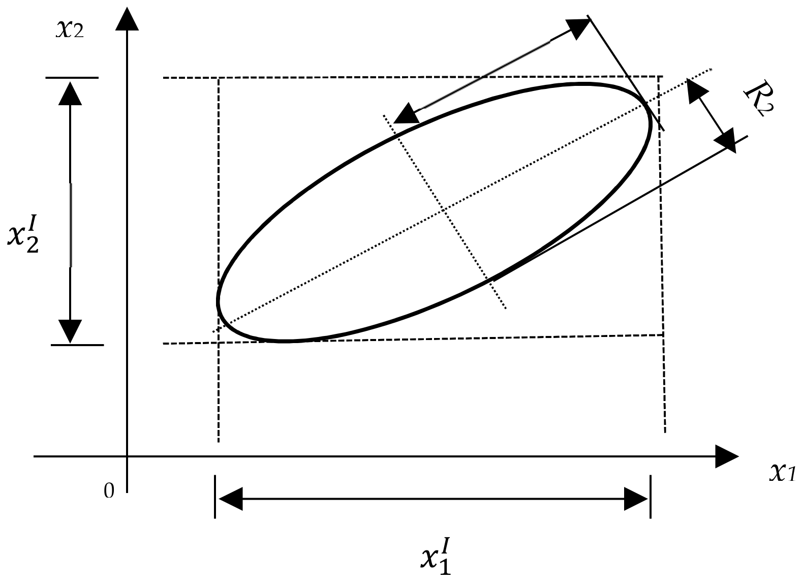
As shown in Figure 3, according to Equation (10), the two-dimensional interaction model can be expressed as:

$$G\left(x\right)={\left(x-x^{\mathrm{c}}\right)}^{\mathrm{T}}{C}^{-1}\left(x-x^{\mathrm{c}}\right)\le 1.$$

(17)

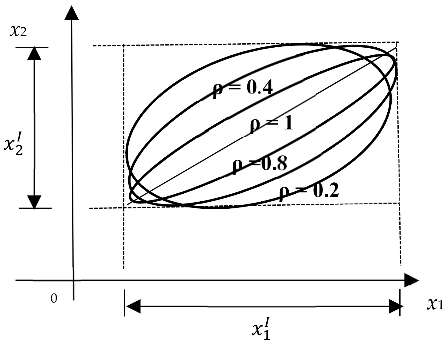
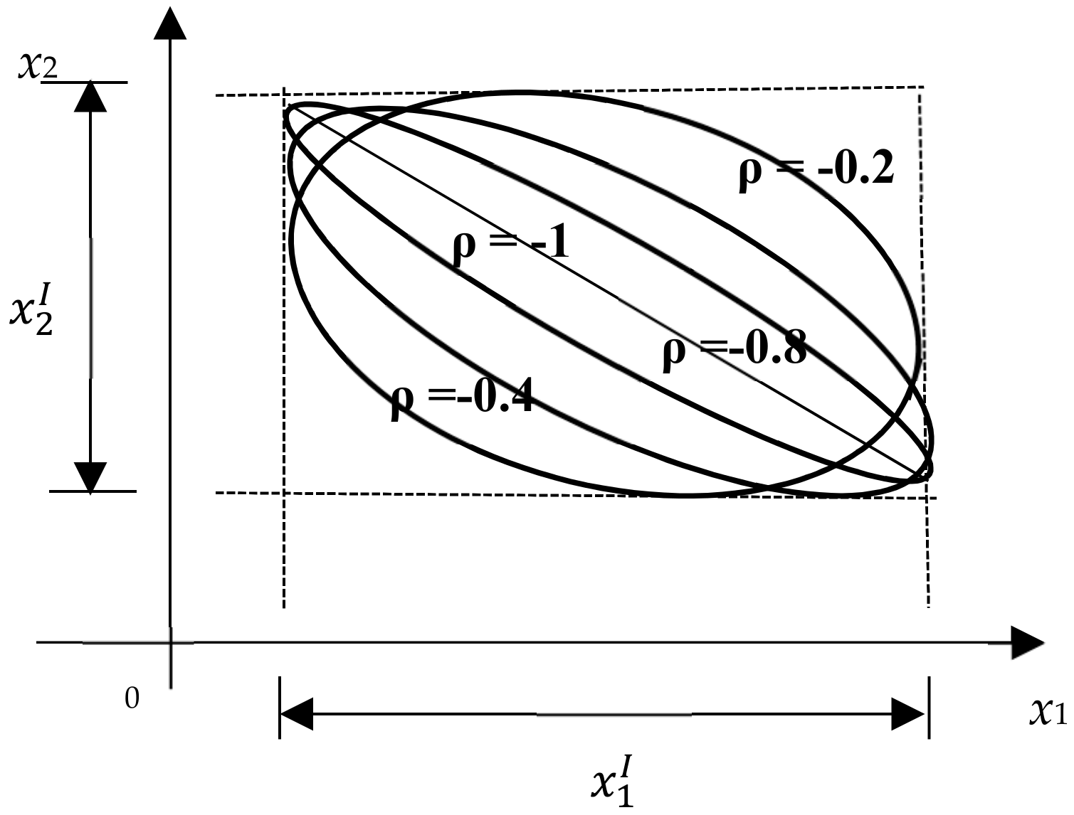
3.3. Interaction Coefficient of Two-Dimensional Interaction Model

The interaction coefficient reflects the geometric characteristics between the uncertain domains. For the interaction model, the magnitude of ${\rho }_{x_1{x}_2}$ reflects the relationship between x₁ and x₂. In addition, a positive interaction of interval variables x₁ and x₂ in two-dimensional ellipsoidal uncertainty fields is shown in Figure 4, while Figure 5 shows a negative correlation of interval variables x₁ and x₂ in two-dimensional interaction uncertainty domains.

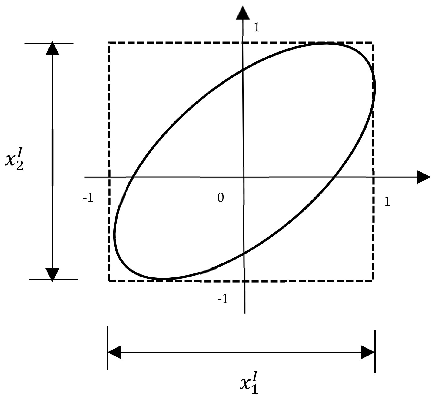
3.4. Standardization of Two-Dimensional Interaction Model

In the two-dimensional space, the interval variable $\left[x_i^{\mathrm{l}},x_i^{\mathrm{u}}\right]$ can be standard quantified as follows:

$$\left[x_1^{\mathrm{l}},x_1^{\mathrm{u}}\right]=\left[x_1^{\mathrm{o}}-x_1^{\mathrm{r}},x_1^{\mathrm{o}}+x_1^{\mathrm{r}}\right],$$

(18)

$$\left[x_2^{\mathrm{l}},x_2^{\mathrm{u}}\right]=\left[x_2^{\mathrm{o}}-x_2^{\mathrm{r}},x_2^{\mathrm{o}}+x_2^{\mathrm{r}}\right].$$

(19)

The uncertainty domains of the two-dimensional interaction model are established [18]:

$$C={\left[\begin{array}{c}{x}_1-x_1^c\\ x_2-x_2^c\end{array}\right]}^{\mathrm{T}}\left[\begin{array}{cc}{\mathrm{cov}}_{x_1{x}_1}& {\mathrm{cov}}_{x_1{x}_2}\\ {\mathrm{cov}}_{x_2{x}_1}& {\mathrm{cov}}_{x_2{x}_2}\end{array}\right]\left[\begin{array}{c}{x}_1-x_1^c\\ x_2-x_2^c\end{array}\right].$$

(20)

Thus, the standardized two-dimensional interaction model, as shown in Figure 6, can be realized as:

$$C={\left[\begin{array}{c}\frac{x_1-x_1^c}{x_1^r}\\ \frac{x_2-x_2^c}{x_2^r}\end{array}\right]}^{\mathrm{T}}\left[\begin{array}{cc}1& {\rho }_{x_1{x}_2}\\ {\rho }_{x_2{x}_1}& 1\end{array}\right]\left[\begin{array}{c}\frac{x_1-x_1^c}{x_1^r}\\ \frac{x_2-x_2^c}{x_2^r}\end{array}\right].$$

(21)

3.5. Definition of N Dimensional Interaction Model for Corroded Defect

When uncertainty parameters constitute an n-dimensional parameter space, all uncertainty parameters x_i can be defined as:

$$\left[x_i^{\mathrm{l}},x_i^{\mathrm{u}}\right]=\left[x_i^0-x_i^{\mathrm{r}},x_i^0+x_i^{\mathrm{r}}\right],i=1,2,3\dots n.$$

(22)

As shown in Figure 7, when correlation exists among these uncertainty parameters, the n-dimensional interaction model can be obtained:

$$M=\left[\begin{array}{cccc}\mathrm{cov}\left(x_1,x_1\right)& \mathrm{cov}\left(x_1,x_2\right)& \cdots & \mathrm{cov}\left(x_1,x_n\right)\\ \mathrm{cov}\left(x_2,x_1\right)& \mathrm{cov}\left(x_2,x_2\right)& \cdots & \mathrm{cov}\left(x_2,x_n\right)\\ ⋮& \cdots & \cdots & ⋮\\ \mathrm{cov}\left(x_n,x_1\right)& \cdots & \cdots & \mathrm{cov}\left(x_n,x_n\right)\end{array}\right],$$

(23)

$${\left(X-X_0\right)}^{\mathrm{T}}{M}^{-1}\left(X-X_0\right)\le 1.$$

(24)

4. Non-Probabilistic Time-Varying Reliability of Ellipsoidal Model with Correlation

4.1. Non-Probabilistic Reliability Analysis

With regards the reliability analysis, the functional equation of structure can be constructed as:

$$Z={\displaystyle \sum _{i=1}^n{R}_i}-{\displaystyle \sum _{i=1}^n{S}_i}(\mathrm{n}=1,2,3\dots \mathrm{n}),$$

(25)

where $Z$ is the structural function, $R$ is the structural resistance, and $S$ is the load effect.

The measurement models of uncertainty domains are different, thus the standardized way is also different. When the interval is $\left[x_i^{\mathrm{L}},x_i^{\mathrm{R}}\right]$, the geometric characteristics of the model can be defined as:

$$x_i^{\mathrm{c}}=\frac{x_i^{\mathrm{L}}+x_i^{\mathrm{R}}}{2},$$

(26)

$$x_i^{\mathrm{r}}=\frac{x_i^{\mathrm{R}}-x_i^{\mathrm{L}}}{2}.$$

(27)

The standardized transformation of the parameters are:

$$U_i=\frac{x_i-x_i^{\mathrm{c}}}{x_i^{\mathrm{r}}},i=1,2,3\dots \mathrm{n}.$$

(28)

Then Equation (24) can be expressed as [30]:

$$U{C}_{\mathrm{U}}^{-1}{U}^{{\rm T}}\le 1.$$

(29)

Substituting Equation (29) into the space of the circle, we can obtain Equation (30), which performs a Cholesky decomposition to a positive definite matrix $C_U^{-1}$:

$$C_{\mathrm{U}}^{-1}=C{C}^{\mathrm{T}}.$$

(30)

When introducing the hypothesis, the expression has the following form:

$$\delta =C^{\mathrm{T}}U.$$

(31)

The standard reliable domain can be obtained using uncertainty domains in the standard circle space:

$${\Omega }=\delta {\delta }^{-1}\le 1.$$

(32)

As shown in Figure 8, when establishing an interaction model based on an ellipsoid theory, the physical meaning of $\beta$ is the expansion space of the standardized interval variable. Thus, the value of the minimum two norm measures the shortest distance from the origin of the coordinate to the failure surface.

Therefore, the optimization equation is then created to compute the non-probabilistic reliability index $\beta$, as follows:

$$\beta =\underset{\delta }{\min }{\Vert \delta \Vert }_2=\min \sqrt{{\delta }_1^2+{\delta }_2^2+\cdots +{\delta }_n^2},$$

(33)

$$\mathrm{s}.\mathrm{t}. f\left(\delta \right)=0,$$

(34)

where ${\Vert \delta \Vert }_2$ is the value of the minimum two norm.

4.2. Non-Probabilistic Time-Dependent Reliability Model

Time-dependent reliability refers to the dynamic reliability of the structure suffered from uncertainty effect over time. Moreover, affects include the varying loads, environmental conditions and degradation of material properties. In real engineering, the effect and the resistance have time-varying characteristics. Therefore, taking into account the time factor for structural reliability is more accurate for reliability analysis. Considering the time-varying characteristics of resistance and effect, the time-varying model can be expressed as:

$$R{\left(T\right)}^{{\rm I}}-S{\left(T\right)}^{{\rm I}}=Z{\left(T\right)}^{{\rm I}},$$

(35)

where $Z{\left(T\right)}^{{\rm I}}$ is the interval of structural function, $R{\left(T\right)}^{{\rm I}}$ is the interval of structural resistance, and $S{\left(T\right)}^{{\rm I}}$ is the interval of structural effect.

When the uncertainty domains of interval variables $x_i\left(i=1,2,3\cdots n\right)$ are described as ellipsoid domains, the non-probabilistic indexes can be defined as the minimum distance of two norm between the origin and the limit state surface. In addition, it can be obtained based on the mathematical optimization theory [31]:

$$\beta =\underset{\partial }{\min }{\Vert \partial \Vert }_2=\min \sqrt{{\partial }_1^2+{\partial }_2^2+\cdots {\partial }_n^2},$$

(36)

$$\mathrm{s}.\mathrm{t}. G(\partial )=0.$$

(37)

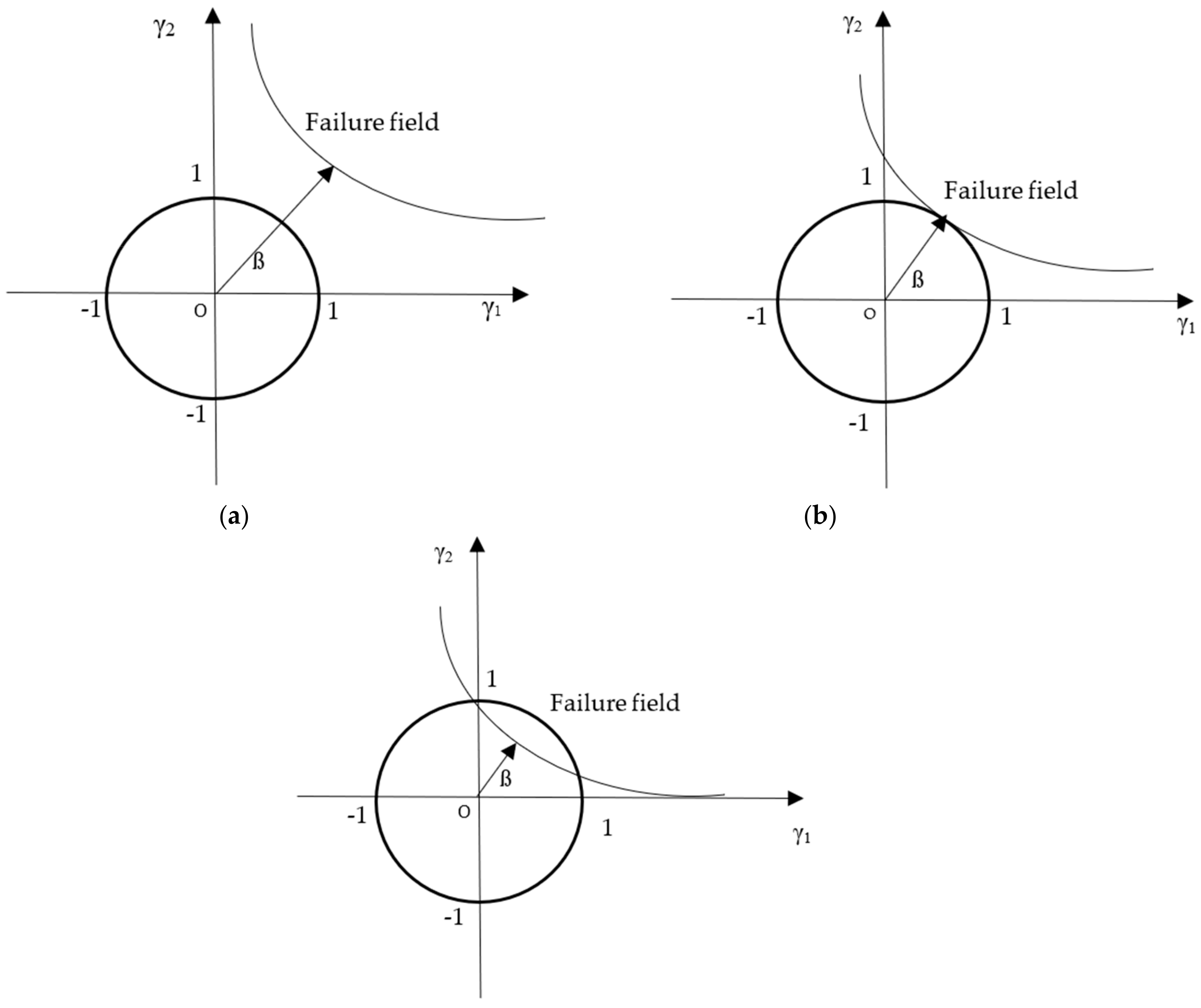
As shown in Figure 9, there are three conditions of non-probabilistic index, which are $\beta >1$, $\beta =1$, and $\beta <1$, respectively. When $\beta >1$, the uncertainty domain and failure domain have no interaction, so the structure is safe. When $\beta =1$, the uncertainty domain and failure surface are tangent to each other, so the structure is located in the critical state. When $\beta <1$, the uncertainty domain and failure surface have partial intersection. Due to the structure having the possibility of failure, it is regarded as losing effectiveness in real engineering. Thus, the degree of reliability and the magnitude of the non-probabilistic reliability index are positively related.

4.3. Reliability Analysis of Corroded Pipelines Under Uncertainty Variables

In order to evaluate the reliability of the corroded pipeline, it is necessary to establish a limit state function which satisfies the structure. Therefore, the reliability analysis needs to determine the uncertainty domain of variables. The definition of the boundaries between pipeline safety and failure is necessary in the reliability analysis. When using $x_i(x_1,x_2,x_3\dots x_n)$ to represent the basic variable, the safety of the pipeline is affected by an uncertain domain. Thus, the limit state equation of the corroded pipeline can be defined as:

$$Z=g(x_1,x_2,x_3\dots x_n).$$

(38)

For the two interrelated uncertainty variables, their projections on the two-dimensional coordinate planes is ellipse. Theoretically, when referring to the three-dimensional space, it can constitute the ellipsoid. Combined with Section 2.3 and Section 4.2, the limit state equation of the corroded pipeline can be proposed as:

$$Z=2\left({\sigma }_s+68.95\right)\frac{w}{D}\times \frac{1-0.85\left(d_0+v_d\Delta T\right)/w}{1-0.85\left(d_0+v_d\Delta T\right)/\left(w{M}_T\right)}-P,$$

(39)

where P is the work pressure of pipelines.

When these uncertain coefficients are described as interval variables with correlation, an optimization equation can be established to obtain a non-probabilistic reliability index:

$$\beta =\min {\Vert \delta \Vert }_2,$$

(40)

$$\mathrm{s}.\mathrm{t}. x_i\in \left[x_i^{\mathrm{l}},x_i^{\mathrm{u}}\right],G(\partial )=0,$$

(41)

where ${\Vert \delta \Vert }_2$ is the distance of two norm and $G(\partial )$ is the limit state surface.

4.4. Non-Probabilistic Reliability Analysis of Multiple Corroded Defects

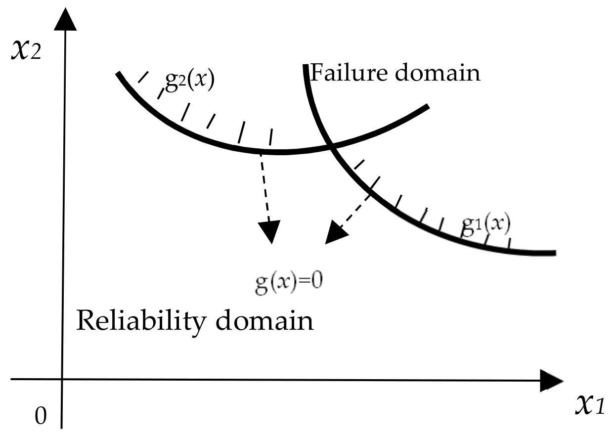
Considering a pipeline containing multiple corroded defects, the non-probabilistic reliability system is series. Thus, the failure of any one of the limit state functions would lead to the failure of the structure. After obtaining the failure modes of each component failure, a calculation of the non-probabilistic reliability index of the structural system can be performed. Taking the system reliability into consideration, the reliability of the structural system is determined by the most dangerous failure mode of the minimum index of non-probability reliability, as shown in Figure 10. Then, the non-probabilistic reliability index of the structural system can be represented in the following form [32]:

$$\beta =\min \left\{{\beta }_1,{\beta }_2,\dots ,{\beta }_n\right\}\ge 0,$$

(42)

where ${\beta }_i\left(i=1,2,3,\dots ,n\right)$ is the non-probabilistic reliability index of the ith failure mode.

5. Examples and Discussion

This section illustrates the impact of the different uncertain variables described herein on the reliability of pipeline. Through the analysis of the associated uncertain variables, the non-probabilistic time-dependent reliability index of the corroded pipeline with interaction is obtained. Considering a pipeline system with multiple corroded defects, the system non-probabilistic reliability is analyzed. Since a three-dimensional interaction model was proposed to study the interaction of multiple variables, which is a study of multi-state reliability in which the pipeline suffers both external and internal influences.

5.1. Non-Probabilistic Time-Dependent Analysis Involving Two Interaction Variables for Corrode Defect

Considering the influences of three conditions relating to the different stochastic variables, the uncertainty variables are constituted using a two-dimensional ellipsoid model. In addition, the basic parameters of pipeline, for these conditions, are shown in

Table 1. Basic parameters of corroded pipeline.

Parameters	Parameter Value
Operating pressure/MPa	2.7
Wall thickness/mm	6.5
Diameter of pipeline/mm	526
Initial depth of defect/mm	[1.9,2.9]
Initial length of defect/mm	[290,310]
Axial corrosion defects growth rate/(mm/year)	14
Radial corrosion defects growth rate/(mm/year)	0.1
Yield stress/MPa	332

,

Table 2. Basic parameters of corroded pipeline.

Parameters	Parameter Value
Operating pressure/MPa	2.7
Wall thickness/mm	6.5
Diameter of pipeline/mm	526
Initial depth of defect/mm	1.9
Initial length of defect/mm	290
Axial corrosion defects growth rate/(mm/year)	[14,16]
Radial corrosion defects growth rate/(mm/year)	[0.075,0.175]
Yield stress/MPa	332

, and

Table 3. Basic parameters of corroded pipeline.

Parameters	Parameter Value
Operating pressure/MPa	2.7
Wall thickness/mm	[14,16]
Diameter of pipeline/mm	[526,530]
Initial depth of corroded defect/mm	1.9
Initial length of corroded defect/mm	290
Axial corrosion defects growth rate/(mm/year)	14
Radial corrosion defects growth rate/(mm/year)	0.1
Yield stress/MPa	332

, respectively [33].

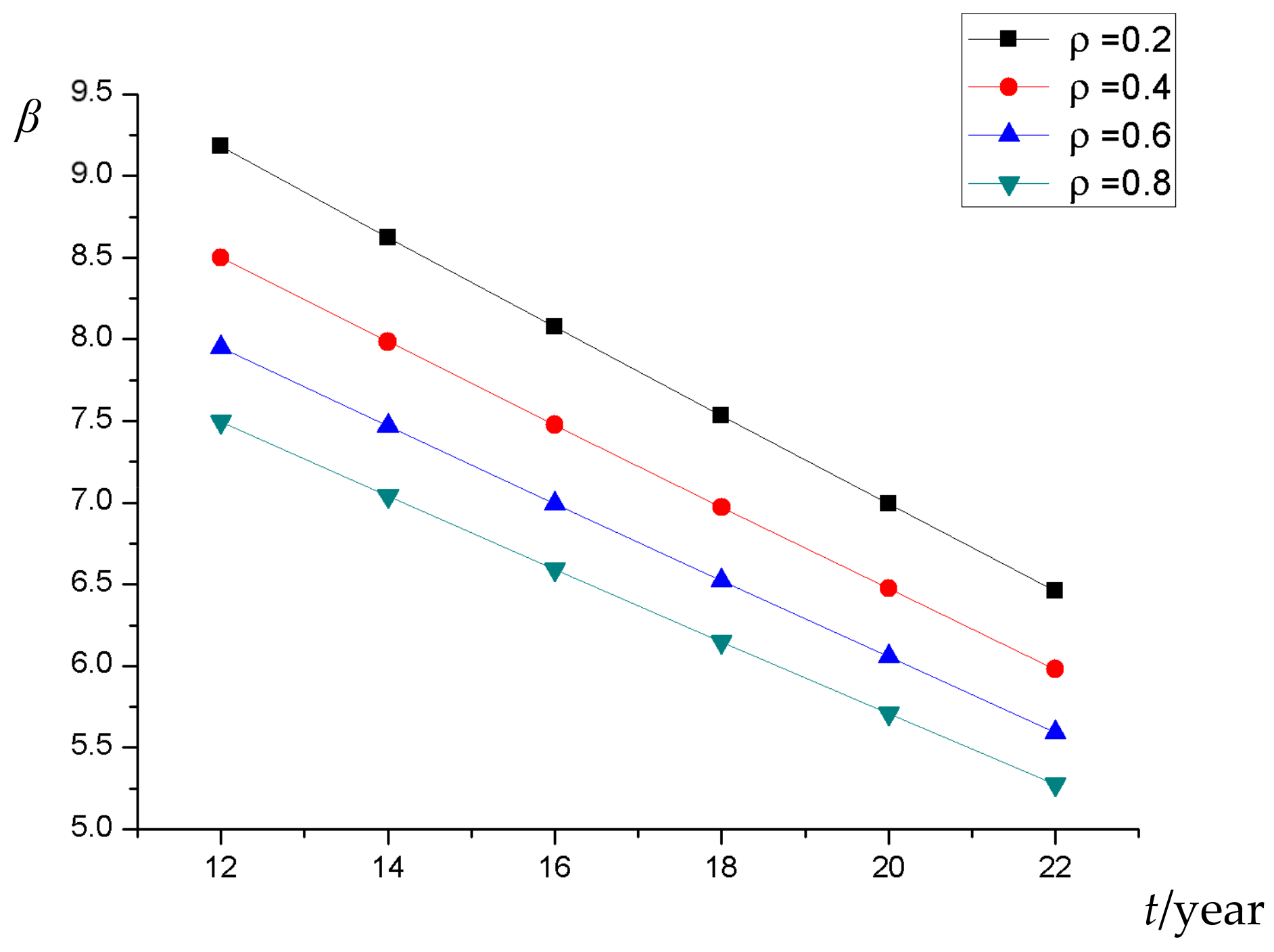
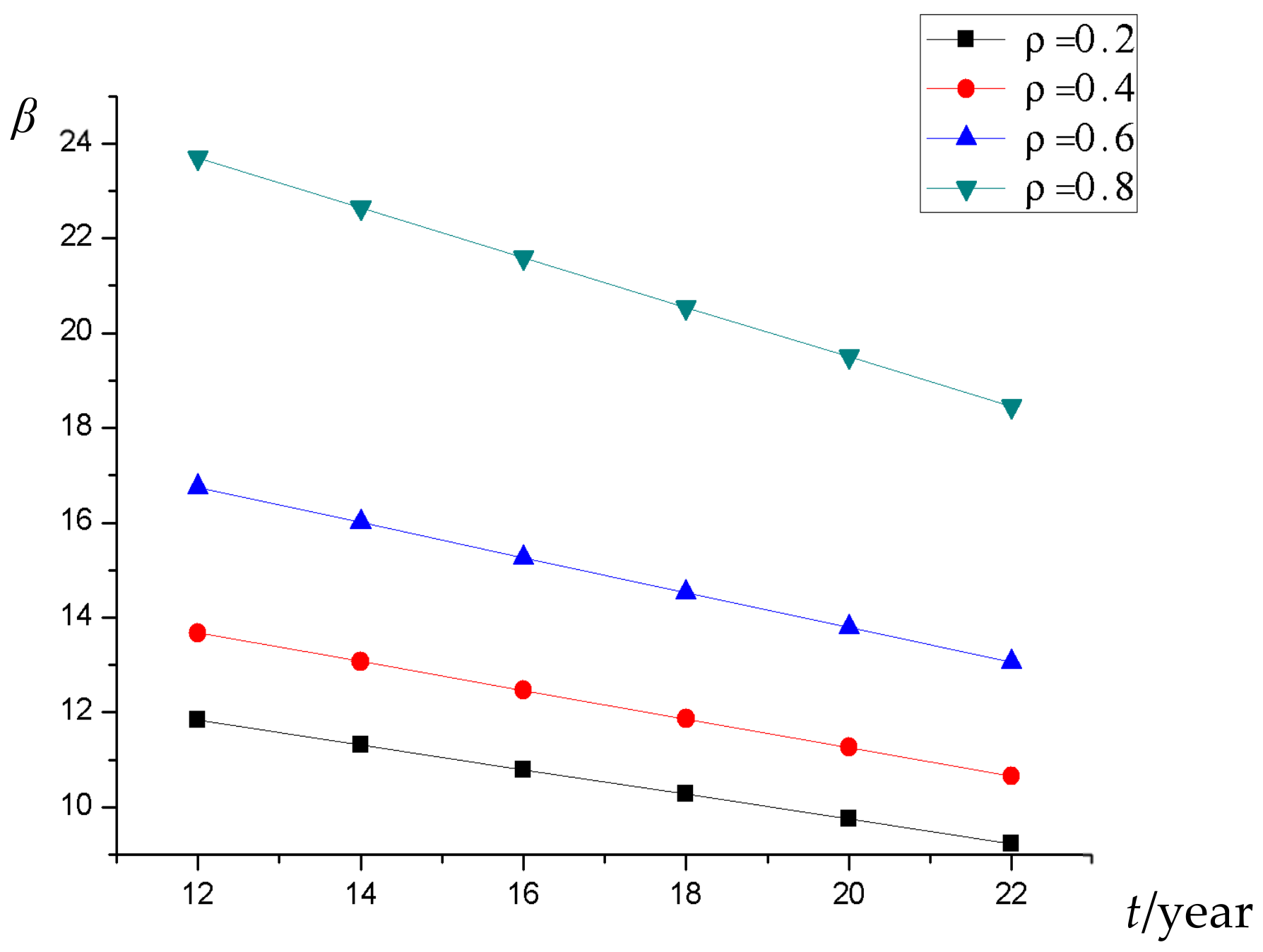
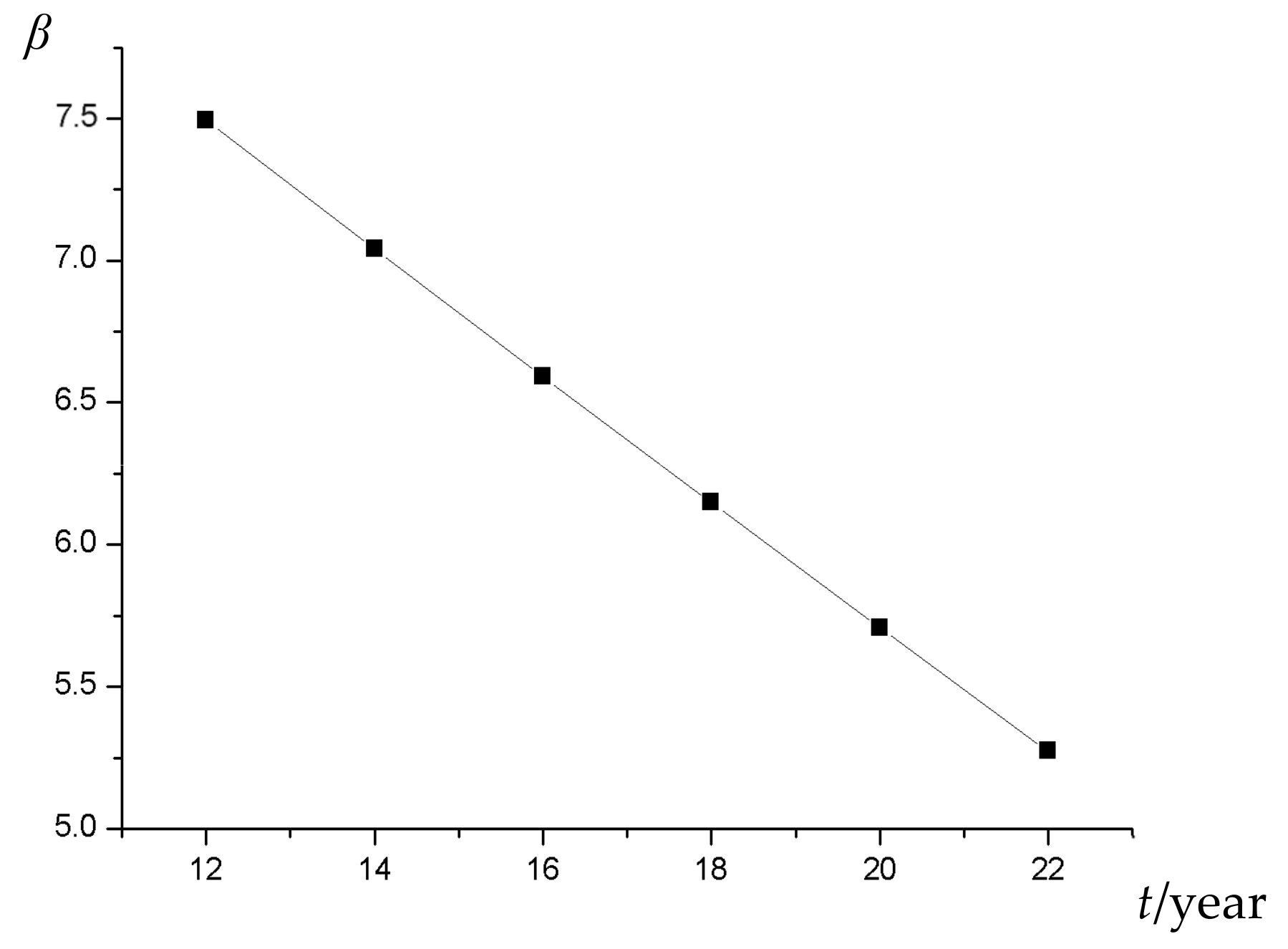
When the interaction coefficients between the two variables in each condition are 0.2, 0.4, 0.6, and 0.8, respectively, other parameters are independent of each other. With the deterioration of time, the non-probabilistic reliability indexes can be calculated as shown in Figure 11, Figure 12, and Figure 13, respectively.

It can be observed that, as shown in Figure 11, Figure 12 and Figure 13, the non-probabilistic reliability indexes show a decreasing trend with time. For locally corroded pipelines, considering the depth and length dependence of corrosion defects, the radial corrosion rate, and the axial corrosion rate, the non-probability reliability index increases with the decreasing of the interaction coefficient, while the non-probability reliability index decreases with the increasing of the interaction coefficient.

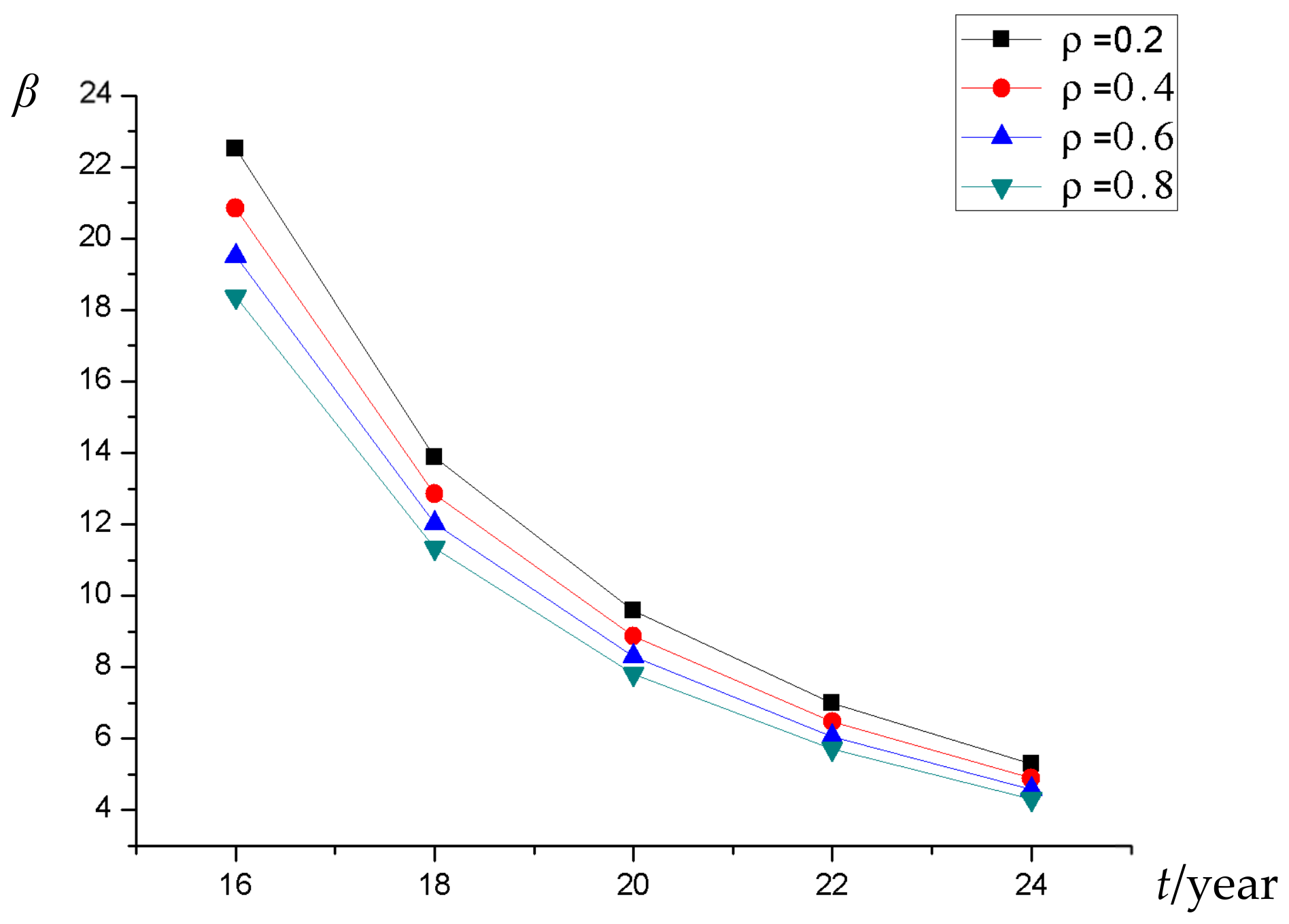
5.2. Non-Probabilistic Time-Dependent System Reliability Analysis of Multiple Corroded Defects

A pipeline has multiple corroded defects during the operation process. Combined with Section 4.4, all parameters of one defect are assumed to be independent while each defect is dependent. For example, the analysis includes each defects’ interaction of depth and length by considering four numbers of defects. The parameters are shown in Table 1. Assuming that the value of interaction coefficient $\rho$ relating to corroded depth of defect and corroded length of defect are 0.2, 0.4, 0.6, and 0.8, respectively, the non-probabilistic time-varying indexes of the pipeline with multiple defects be as shown in Figure 14.

As mentioned, the interaction between multiple adjacent corroded defects leads to a reduction in the reliability of the pipeline, and the reliability is reduced with time. Thus, the mutual influence of multiple corrosion defects will cause the system to reduce the non-probabilistic reliability index.

5.3. Non-Probabilistic Time-Dependent Reliability Analysis Involving Multi-Dimensional Interaction for Corrode Defect

When the pipeline is simultaneously damaged by corrosion damage and natural disasters, the interaction research is three-dimensional.

Table 4. Parameters of suspended pipeline with corrosion defects.

Parameters	Parameter Value
Wall thickness/mm	7.5
Diameter of pipeline/mm	506
Initial depth of corroded defect/mm	[2.2,3.2]
Initial width of corroded defect/mm	[10,12]
Axial corroded defects growth Rate/(mm/year)	0.1
Loop corroded defects growth Rate/(mm/year)	0.2
Suspended length/m	[124,132]

shows the parameters of the X52 suspended pipeline with corroded defects. Combined with the time-dependent reliability model and the limit state equation for a suspended pipeline with corroded pipeline has the following form [34,35,36]:

$$Z=47.453+\frac{5.29\left(d_0+v_d\Delta T\right)}{0.79t}+\frac{1.67}{0.004+\frac{b_0+v_b\Delta T}{0.67\pi D}}-\frac{0.02}{\left(0.004+\frac{d_0+v_d\Delta T}{0.79t}\right)\times \left(0.004+\frac{b_0+v_b\Delta T}{0.67\pi D}\right)}-L_s$$

(43)

Considering the interaction of the corroded depth, corroded width, and suspended length, the matrix of interaction coefficient can be constructed as:

$$\left[\begin{array}{ccc}1& {\rho }_{12}& {\rho }_{13}\\ {\rho }_{21}& 1& {\rho }_{23}\\ {\rho }_{31}& {\rho }_{32}& 1\end{array}\right].$$

(44)

After obtaining the matrix of the interaction coefficient, the three-dimensional interaction model can be expressed as:

$$\left\{\left[\begin{array}{c}{d}_0\\ b_0\\ L_s\end{array}\right]\right\}{\left[\begin{array}{c}\left(d_0-2.7\right)/0.5\\ \left(b-11\right)/1\\ \left(L_s-128\right)/4\end{array}\right]}^{\mathrm{T}}\left[\begin{array}{ccc}1& {\rho }_{12}& {\rho }_{13}\\ {\rho }_{21}& 1& {\rho }_{23}\\ {\rho }_{31}& {\rho }_{32}& 1\end{array}\right]\left[\begin{array}{c}\left(d_0-2.7\right)/0.5\\ \left(b_0-11\right)/1\\ \left(L_s-128\right)/4\end{array}\right]\le 1.$$

(45)

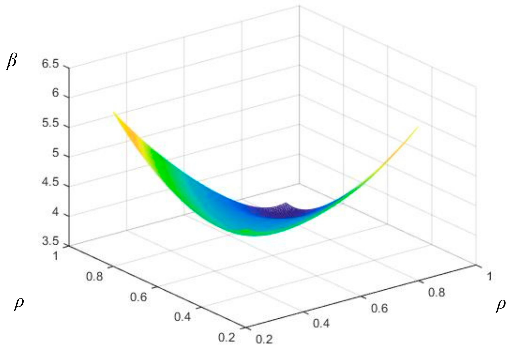
To discuss the influence of multidimensional interaction on the reliability of pipelines, the trend in the presence of a fixed time, i.e.,$t$, is used as a reference. For example, when the time is taken as 12 years, the interaction coefficients among corroded depth, corroded width, and limit suspended length are assumed to be 0.2, 0.4, 0.6, and 0.8, respectively. Furthermore, other random variables are independent of each other. When coefficients ${\rho }_{12}$, ${\rho }_{13}$, ${\rho }_{21}$, ${\rho }_{23}$, ${\rho }_{31}$, ${\rho }_{32}$ are 0.2, the non-probability reliability index is 5.1585; when coefficients ${\rho }_{12}$, ${\rho }_{13}$, ${\rho }_{21}$, ${\rho }_{23}$, ${\rho }_{31}$, ${\rho }_{32}$ are 0.4, the non-probability reliability index is 4.5494; when coefficients ${\rho }_{12}$, ${\rho }_{13}$, ${\rho }_{21}$, ${\rho }_{23}$, ${\rho }_{31}$, ${\rho }_{32}$ are 0.6, the non-probabilistic reliability indicator is 4.1151; and when coefficients ${\rho }_{12}$, ${\rho }_{13}$, ${\rho }_{21}$, ${\rho }_{23}$, ${\rho }_{31}$, ${\rho }_{32}$ are 0.8, the non-probabilistic reliability indicator is 3.7853. The results are shown in Figure 15.

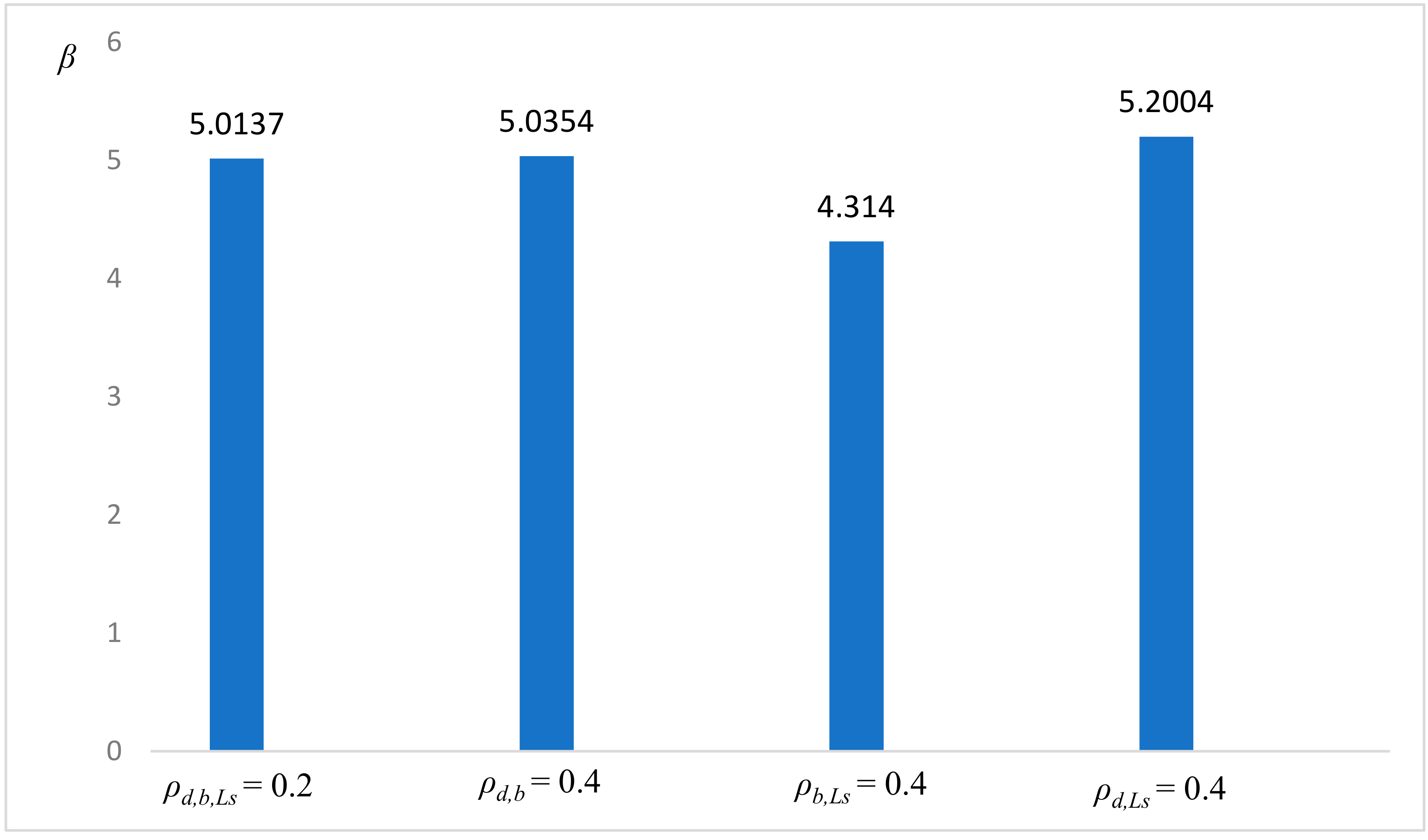
In order to further demonstrate the influence of the interaction degree of different uncertain variables on the pipeline reliability, when the working time of the corroded pipeline is 12 years, this paper establishes an interaction corrosion study under four conditions as follows:

• the values of interaction coefficients for corroded length, corroded depth, and limit suspended length are all 0.2
• the value of interaction coefficients for corroded length and corroded depth is 0.4, the other values of interaction coefficients are all 0.2
• the value of interaction coefficients for corroded depth and limit suspended length is 0.4, the other values of interaction coefficients are all 0.2
• the value of interaction coefficients for corroded width and limit suspended length is 0.4, the other values of interaction coefficients are all 0.2
• the results in Figure 16 compare the non-probabilistic reliability indexes in these four cases.

It can be observed from Figure 16 that when the value of interaction coefficient for corroded depth, corroded width, and suspended length is 0.2, the non-probabilistic index is 5.1585. However, when the value of the interaction coefficient for corroded defect is changed to 0.4, the non-probabilistic index is 5.0354. Similarly, when the interaction coefficient of corroded width and suspended length is 0.4, the non-probabilistic index is 4.3140, and when the interaction coefficient of corroded depth and suspended length is 0.4, the non-probabilistic index is 5.2004. Apparently, as analyzed above, the degree of interaction between corroded width and suspended length has a more significant level than corroded width and corroded depth on the safety of corroded pipelines, while the influence of corroded depth and suspended length is small. Thus, the conclusions drawn apply for corroded pipelines with regards safety inspection and prediction of remaining life.

6. Conclusions

The reliability analysis of corroded pipeline is a bright methodology for defect assessment, especially involving the interaction influence for corroded defects and natural disaster. Based on the small amount of data in some practical engineering, a non-probabilistic ellipsoid model is proposed for uncertainty quantification of uncertain parameters. In addition, corroded pipeline considering interaction is analyzed through the proposed method. Two interaction variables for corroded pipeline can be analyzed by constructing an ellipse model, and three interaction variables by constructing a three-dimensional ellipsoid model.

Thus, the non-probability time-dependent index for pipeline with corroded defects can be calculated using small samples, which would be very helpful for risk- and reliability-formed risk decision in pipeline engineering. With the degree of interaction analysis for interval variables, the sensitivity of related parameters in the reliability analysis is proposed, which is necessary for the safe detection of corroded pipelines. Furthermore, the dynamic time-dependent characteristics and trend of reliability in practical engineering is verified. Considering the multiple defects, a methodology is developed to calculate the non-probabilistic time-dependent index for the system reliability.

It is true that the proposed methodology can be used to establish the limit state equation under the influence of multiple factors based on small samples, which is a supplement to the reliability analysis of pipeline engineering. Moreover, through studying the influence of two and three interaction variables on corroded pipeline, the results show that different variables have different degrees of influence on reliability. This research therefore lays the foundation for a non-probabilistic time-dependent reliability analysis of oil and gas pipelines that takes into account the interaction of corroded defects in reliability analysis and has important engineering significance for risk decision and reliability design of pipeline engineering.

References

- Zhang, P.; Wang, Y.H.; Qin, G.J. Fuzzy damage analysis of the seismic response of a long-distance pipeline under a coupling multi-influence domain. Energies 2019, 12, 62. [Google Scholar] [CrossRef]
- Ndubuaku, O.; Martens, M.; Cheng, J.J.R.; Adeeb, S. Integrating the shape constants of a novel material stress-strain characterization model for parametric numerical analysis of the deformational capacity of high-strength x80-grade steel pipelines. Appl. Sci. 2019, 9, 322. [Google Scholar] [CrossRef]
- Teixeira, A.P.; Soares, C.G.; Netto, T.A.; Estefen, S.F. Reliability of pipelines with corrosion defects. Int. J. Press. Vessel. Pip. 2008, 85, 228–237. [Google Scholar] [CrossRef]
- Mihir, M.; Vahid, K.; Arash, N. Reliability-based lifecycle management for corroding pipelines. Struct. Saf. 2019, 76, 1–14. [Google Scholar] [CrossRef]
- Caleyo, F.; González, J.L.; Hallen, J.M. A study on the reliability assessment methodology for pipelines with active corrosion defects. Int. J. Press. Vessel. Pip. 2002, 79, 77–86. [Google Scholar] [CrossRef]
- Zhang, P.; Su, L.B.; Qin, G.J.; Kong, X.H.; Peng, Y. Failure probability of corroded pipeline considering the correlation of random variables. Eng. Fail. Anal. 2019, 99, 34. [Google Scholar] [CrossRef]
- Chen, H.F.; Shu, D. Simplified limit analysis of pipelines with multi-defects. Eng. Struct. 2001, 23, 207–213. [Google Scholar] [CrossRef]
- Zhou, W.; Xiang, W.; Hong, H.P. Sensitivity of system reliability of corroding pipelines to modeling of stochastic growth of corrosion defects. Reliab. Eng. Syst. Saf. 2017, 167, 428–438. [Google Scholar] [CrossRef]
- Hong, X.B.; Liu, Y.; Lin, X.H.; Luo, Z.Q.; He, Z.W. Nonlinear ultrasonic detection method for delamination damage of lined anti-corrosion pipes using PZT transducers. Appl. Sci. 2018, 8, 2240. [Google Scholar] [CrossRef]
- Al-Amin, M.; Zhou, W. Evaluating the system reliability of corroding pipelines based on inspection data. Struct. Infrastruct. Eng. 2014, 10, 1161–1175. [Google Scholar] [CrossRef]
- Qian, G.; Niffenegger, M.; Zhou, W.X.; Li, S.X. Effect of correlated input parameters on the failure probability of pipelines with corrosion defects by using FITNET FFS procedure. Int. J. Press. Vessel. Pip. 2013, 105, 19–27. [Google Scholar] [CrossRef]
- Larin, O.; Barkanov, E.; Vodka, O. Prediction of reliability of the corroded pipeline considering the randomness of corrosion damage and its stochastic growth. Eng. Fail. Anal. 2016, 66, 60–71. [Google Scholar] [CrossRef]
- Seghier Ben, M.E.A.; Bettayeb, M.; Correia, J. Structural reliability of corroded pipeline using the so-called Separable Monte Carlo method. J. Strain Anal. Eng. Design 2018, 53, 730–737. [Google Scholar] [CrossRef]
- Seghier Ben, M.E.A.; Keshtegar, B.; Correia, J.; Lesiuk, G.; De Jesus, A. Reliability analysis based on hybrid algorithm of M5 model tree and Monte Carlo simulation for corroded pipelines: Case of study X60 Steel grade pipes. Eng. Fail. Anal. 2019, 97, 798–803. [Google Scholar] [CrossRef]
- Ben-Haim, Y.; Elishakoff, I. Convex Models of Uncertainties in Applied Mechanics; Elsevier: Amsterdam, The Netherlands, 1990. [Google Scholar]
- Elishakoff, I.; Elisseeff, P.; Glegg, S.A.L. Non-probabilistic, convex-theoretic modeling of scatter in material properties. Aiaa J. 2012, 32, 843–849. [Google Scholar] [CrossRef]
- Zeng, M.; Hao, H.; Zhou, H.L. Super parametric convex model and its application for non-probabilistic reliability-based design optimization. Appl. Math. Modell. 2018, 55, 354–370. [Google Scholar] [CrossRef]
- Ni, B.Y.; Jiang, C.; Huang, Z.L. Discussions on non-probabilistic convex modelling for uncertain problems. Appl. Math. Modell. 2018, 59, 54–85. [Google Scholar] [CrossRef] [Green Version]
- Jiang, C.; Han, X.; Lu, G.Y.; Liu, J.; Zhang, Z.; Bai, Y.C. Correlation analysis of non-probabilistic convex model and corresponding structural reliability technique. Comp. Methods Appl. Mech. Eng. 2011, 200, 2528–2546. [Google Scholar] [CrossRef]
- Pantelides, C.P.; Ganzerli, S. Design of trusses under uncertain loads using convex models. J. Struct. Eng. 1998, 124, 318–329. [Google Scholar] [CrossRef]
- Li, J.; Chen, J.B.; Fan, W.L. The equivalent extreme-value event and evaluation of the structural system reliability. Struct. Saf. 2007, 29, 112–131. [Google Scholar] [CrossRef]
- Utkin, L.V.; Gurov, S.V. A general formal approach for fuzzy reliability analysis in the possibility context. Fuzzy Sets Syst. 1996, 83, 203–213. [Google Scholar] [CrossRef]
- Liu, J.; Zio, E. System dynamic reliability assessment and failure prognostics. Reliab. Eng. Syst. Saf. 2017, 160, 21–36. [Google Scholar] [CrossRef] [Green Version]
- Xu, L.Y.; Cheng, Y.F. Reliability and failure pressure prediction of various grades of pipeline steel in the presence of corrosion defects and pre-strain. Int. J. Press. Vessel. Pip. 2012, 89, 75–84. [Google Scholar] [CrossRef]
- Leis, B.; Stephens, D. An Alternative Approach to Assess the Integrity of Corroded Line Pipe—Part I: Current Status; International Society of Offshore and Polar Engineers: Whisam, CA, USA, 1997. [Google Scholar]
- Kiefner, J.F.; Vieth, P.H. Evaluating pipe 1: New method corrects criterion for evaluating corroded pipe. Oil Gas J. 1990, 88, 56–59. [Google Scholar] [CrossRef]
- American Society of Mechanical Engineers (ASME) B31G. Manual for Determining the Remaining Strength of Corroded Pipelines; American Society of Mechanical Engineers (ASME): New York, NY, USA, 2009. [Google Scholar]
- Caleyo, F.; Velázquez, J.C.; Valor, A.; Hallena, J.M. Probability distribution of pitting corrosion depth and rate in underground pipelines: A Monte Carlo study. Corros. Sci. 2009, 51, 1934. [Google Scholar] [CrossRef]
- Jiang, C.; Bi, R.G.; Lu, G.Y.; Han, X. Structural reliability analysis using non-probabilistic convex model. Comp. Methods Appl. Mech. Eng. 2013, 254, 83–98. [Google Scholar] [CrossRef]
- Wang, B.; Jiang, C. Reliability analysis method of evidence theory structure considering correlation. Mech. Sci. Technol. 2014, 33, 1324–1328. [Google Scholar] [CrossRef]
- Luo, Y.J.; Kang, Z.; Li, A. Research on structural non-probabilistic reliability index based on convex model and its solving method. J. Solid Mech. 2011, 32, 646–654. [Google Scholar] [CrossRef]
- Qiu, Z.P.; Yang, D.; Elishakoff, I. Probabilistic interval reliability of structural systems. Int. J. Solids Struct. 2008, 45, 2850–2860. [Google Scholar] [CrossRef] [Green Version]
- Wei, Z.P. Dynamic non-probabilistic reliability analysis of corroding pipelines in service. J. Eng. Design 2014, 21, 27–31. [Google Scholar] [CrossRef]
- Wang, Y.H.; Zhang, P.; Qin, G.J. Non-probabilistic time-dependent reliability analysis for suspended pipeline with corrosion defects based on interval model. Process Saf. Environ. Protect. 2019, 124, 290–298. [Google Scholar] [CrossRef]
- Liu, Z.; Liu, Y.; He, B.J.; Xu, W.; Jin, G.; Zhang, X. Application and suitability analysis of the key technologies in nearly zero energy buildings in China. Renew. Sust. Energ. Rev. 2019, 101, 329–345. [Google Scholar] [CrossRef]
- Zhang, P.; Qin, G.; Wang, Y. Risk Assessment System for Oil and Gas Pipelines Laid in One Ditch Based on Quantitative Risk Analysis. Energies 2019, 12, 981. [Google Scholar] [CrossRef]
Figure 1.
Local corrosion.
Figure 2.
The profile of pipeline with ideal corrosion defects.
Figure 3.
Two-dimensional interaction model for corroded defect.
Figure 4.
Two-dimensional ellipsoidal uncertainty domain of positive interaction coefficient.
Figure 5.
Two-dimensional ellipsoidal uncertainty domain of negative interaction coefficient.
Figure 6.
The standardized two-dimensional interaction model.
Figure 7.
Three-dimensional interaction model.
Figure 8.
Non-probabilistic reliability index of the standard space ellipsoid model.
Figure 9.
State of structure: (a) the structure is safe, ; (b) the structure is critical state, ; (c) the structure has possibility of failure, .
Figure 10.
Failure surfaces of the series systems.
Figure 11.
Non-probabilistic non-varying reliability indexes considering the interaction of corroded length and depth.
Figure 12.
Non-probabilistic time-varying reliability indexes considering axial corrosion defects, growth rate, and radial corrosion defects growth rate.
Figure 13.
Non-probabilistic time-varying reliability index considering diameter and wall thickness.
Figure 14.
Non-probabilistic time-varying system reliability analysis.