Comparison of Direct and Indirect Active Thermal Energy Storage Strategies for Large-Scale Solar Heating Systems


1
ESIEE Paris, University of Paris Est, F-93162 Noisy le Grand, France
2
LIED-PIERI, UMR 8236, CNRS, University of Paris Diderot (Paris 7), F-75013 Paris, France
3
EFFICACITY, 14-20 boulevard Newton, F-77447 Marne la Vallée CEDEX 2, France
4
Jiangsu Provincial Key Laboratory of Oil & Gas Storage and Transportation Technology, Changzhou University, Changzhou, Jiangsu 213016, China
*
Authors to whom correspondence should be addressed.
Energies 2019, 12(10), 1948; https://doi.org/10.3390/en12101948
Submission received: 3 April 2019
/
Revised: 15 May 2019
/
Accepted: 16 May 2019
/
Published: 21 May 2019
(This article belongs to the Special Issue Solar Thermal Energy Storage and Conversion)
Abstract
:Large-scale solar heating for the building sector requires an adequate Thermal Energy Storage (TES) strategy. TES plays the role of load shifting between the energy demand and the solar irradiance and thus makes the annual production optimal. In this study, we report a simplified algorithm uniquely based on energy flux, to evaluate the role of active TES on the annual performance of a large-scale solar heating for residential thermal energy supply. The program considers different types of TES, i.e., direct and indirect, as well as their specifications in terms of capacity, storage density, charging/discharging limits, etc. Our result confirms the auto-regulation ability of indirect (latent using Phase Change Material (PCM), or Borehole thermal storage (BTES) in soil) TES which makes the annual performance comparable to that of direct (sensible with hot water) TES. The charging and discharging restrictions of the latent TES, until now considered as a weak point, could retard the achievement of fully-charged situation and prolong the charging process. With its compact volume, the indirect TES turns to be promising for large-scale solar thermal application.
1. Introduction
Recovery and Renewable Energy Sources (RRES) are abundant in urban areas where the principal energy demands come from the building sector. While building energy renovation is encouraged by recent European directives [1], its pace is far from satisfactory. In 2016, the annual renovation rate in the EU countries is 0.4–1.2% whereas still 75% of the remaining house stock is yet to be restored. In the middle term, injecting RRES in heating and Domestic Hot Water (DHW) supply provides opportunity to reduce fossil dependency and carbon emissions from buildings.
Meanwhile, technical and legislative supports in District Heating Networks (DHN) development provide favourable conditions for RRES integration. First, the next generation DHN will be characterized by low temperature thermal energy supply [2,3]. Contrary to typical high temperature solutions such as that with steam (1st generation) or pressurised hot water above 100 °C (2nd and 3rd generation), the supply temperature of the 4th generation DHN is lower than 100 °C. This trend is ongoing thanks to techniques like Demand Side Management (DSM) through building thermal mass [4,5], load prediction & scheduling [6], using thermally responsive coatings to regulate the solar input [7], as well as online substation monitoring & control [8,9]. In consequence, several low-grade RRES (e.g., solar thermal, sewage water heat recovery) could find their place in modern DHN. Secondly, governmental regulations have been established in most EU countries encouraging DHN energy efficiency progress [10,11]. In France, local authorities can impose purchase obligations on new construction buildings to connect their energy distribution systems to an existing DHN [11]. Other legislative supports include reduced taxes and heat funds from ADEME [12] for new DHN projects. Finally, to benefit from the above legislative supports, one important condition is that the DHN’s RRES share into the global energy mix should be at least 50%. For this reason, both energy service companies and local authorities are looking for RRES integration in their DHN project development.
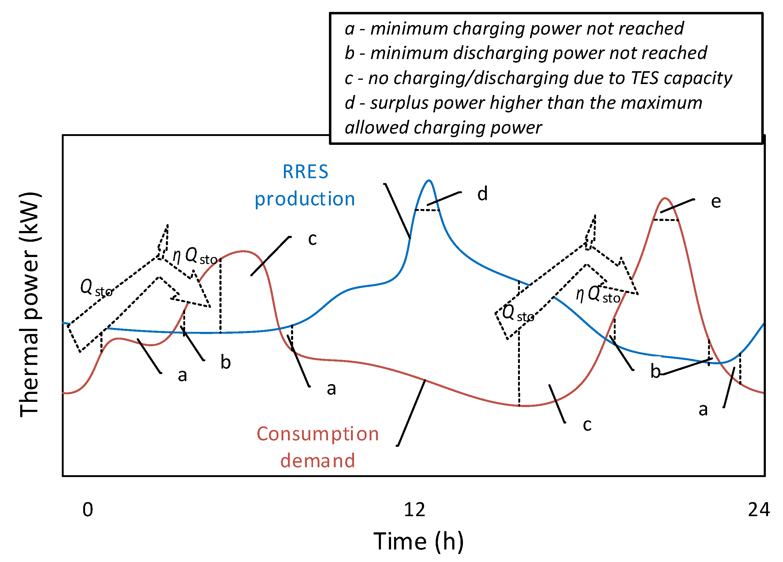
Although the reported amount of low-temperature RRES is significant, their deployment requires very cautious study. A decision-making tool with compromise between heavy computing simulation and rough estimation is highly needed. First, traditional estimation methods tend to over-estimate the available energy quantity. In France, statistical top-down estimations give around 100 TWh of waste heat in the manufacturing industry for a temperature range between 40 and 250 °C [13]. Similarly in the UK, the waste recovery estimation is between 10 TWh and 40 TWh between ambient temperature and 250 °C [14,15]. These estimations are significant, since a decrease from 75% to 50% of French national nuclear electricity production in 2013 means around 140 TWh [16]. If all waste heat were reused, a profound change in the energy landscape would have been realized. However, the above-mentioned estimation of waste heat availability is done with high improbability. According to Brueckner et al. [17], potential estimation of waste heat resources decreases from a physical estimation to technical one, until down to an economically acceptable value. The top-down approach, largely used by related studies [13,14,15,18], is not adapted for a specific project evaluation. Then, the spatial distance and temporal variation characteristics of waste sources with respect to potential user’s demands make some available RRES not effectively used. The mismatching between intermittent sources and fluctuating demands can be shown in Figure 1. In case of high RRES penetration in a DHN, ideal thermal energy storage (TES) system can shift the surplus to later consumption. The ideal case supposes that the TES can store surplus energy production and release it entirely later when demand dominates production. The share of sustainable energy in total annual energy consumption can approach its maximum potential value. To be more realistic, a rigorous analysis as explained by legends a/b/c/d of the Figure 1 should be adopted. In this detailed analysis, one should consider TES capacity (shown as c in the figure) and the storage efficiency η. The minimum and maximum charging/discharging rate limitation (shown as a/b/d/e in the figure), should also be accounted.
The objective of this study is to investigate the influence of TES integration in a DHN with high RRES penetration, taking solar thermal as an example. The idea is to develop an easy-to-use decision-making tool for solar thermal deployment in a low-carbon city, without employing highly complex simulation tools. Specifically, we consider the annual dynamic energy curves of both demand- and source-sides with an hourly time step. The mismatching is treated by TES integrations and we compare two types of TES with different sizing. Yet rarely addressed by the literature, the charging and discharging limitations of latent (indirect) and sensible (direct) TES are considered in this work. The study is part of a large project within EFFICACITY, a French national research institute focusing on urban energy transition [19]. The decision-making tool is named Recov’Heat [20] and it provides techno-economic indicators with only a limited number of key parameters. By using this tool, local communities and energy service companies can easily make preliminary studies with sufficient precision about the feasibility of solar thermal district heating project. This open-access tool [21] helps break the barrier of pre-study costs while delivering sufficiently accurate results for project implementation.
The manuscript is organised as follows: Section 2 briefly reviews different TES systems that can be used in a DHN. Their main characteristics to be considered in the modelling are listed. Section 3 introduces the methodology to construct TES integrated estimation model as well as demand- and production-side thermal energy data to be used as inputs. In Section 4, we analyse the influence of TES capacities based on selected criteria. Special attention is given to the sizing influence on the annual performance in terms of solar share within the total demand and the recovery ratio with respect to a waste heat source. Comparisons are also made between direct hot water-based TES and indirect TES using a Phase Change Material (PCM). Finally, a comparative techno-economic analysis is done to evaluate the energy cost and CO2 emission with/without TES.
2. TES Systems: Position, Characteristics and Classification
Different TES systems, from hourly to seasonal storage, from centralized installation to individual small-size equipment, have been extensively used. The most known TES system is perhaps electric hot water tanks with sizing of about a hundred litres, generally installed in individual households in high electrification countries like France. The heat storage tank enables a lower electricity bill for householders by allowing heating during off-peak hours when most grid companies charge lower tariffs. Besides, cumulative heating mode can avoid grid pollution from excessive power demand, which is the case for instantaneous electric heaters. Besides, solar thermal and air source heat pump heaters also require storage tank due to their low heating power. Others TES are on greater scales, such as storage in aquifer (ATES) or borehole (BTES). Those large-scale systems have been extensively tested particularly in solar thermal district heating projects through the IEA SHC (International Energy Agency, Solar Heating and Cooling) demonstrational tasks [22].
Depending on their physical mechanisms, TES can be classified by sensible, latent and thermochemical energy storage. Sensible TES uses the heat capacity of a storage medium by raising (charging) or decreasing (discharging) its temperature and conserve the energy during the storage (standby). The storage temperature differs from that of ambient and as a result heat loss should be considered. Advanced TES systems by latent heat using PCM [23] or chemical- or physical-bond related energy, so called thermochemical techniques, have also been studied extensively [24]. PCM and thermochemical storages are usually more compact than sensible TES. In addition, certain storage configurations use the supercooling of certain PCM and thus have zero heat loss during the storage [25]. Each of these systems has its own pros and cons from different criteria. From the point of view of system integration and for any of the above storage technologies, a TES should be:
- (i)
- Reliable and flexible: energy could be charged and retrieved with sufficient intensity (charging/discharging rates) whenever demanded;
- (ii)
- Efficient: charged energy should be recovered with low heat loss during storage;
- (iii)
- Available at the right temperature level. This criterion applies mainly to sensible, liquid-based TES where fluids with different temperature levels can be mixed if the storage volume is not well stratified. A perfect stratification can be supposed only if the natural convection is mastered and no turbulence created during charging/discharging processes.
In this study, both direct (hot water) and indirect (typically PCM or BTES) active TES are addressed. We define direct TES by those who don’t rely on an intermediate Heat Transfer Fluid (HTF) or heat exchanger in the TES itself. The system takes in general water as the storage medium. Comparatively, the thermal storage medium in an indirect TES cannot flow out of its storage reservoir [26,27,28]. Thus, a HTF is needed to circulate between the heat user (e.g., heat pump) and the storage medium, through a heat exchanger. In this study, their differences in charging/discharging time as well as energy storage density are considered. Particularly for the indirect one, comparing with a direct TES can help evaluate the influence of its charging/discharging rate limitations to the overall performance at the system level. Note that passive buildings using TES in the building envelop is a direct technique but in a passive way; while this paper only addresses the active TES, i.e., a storage reservoir exclusively dedicated for thermal storage purpose.
2.1. Position of TES in Heating Networks
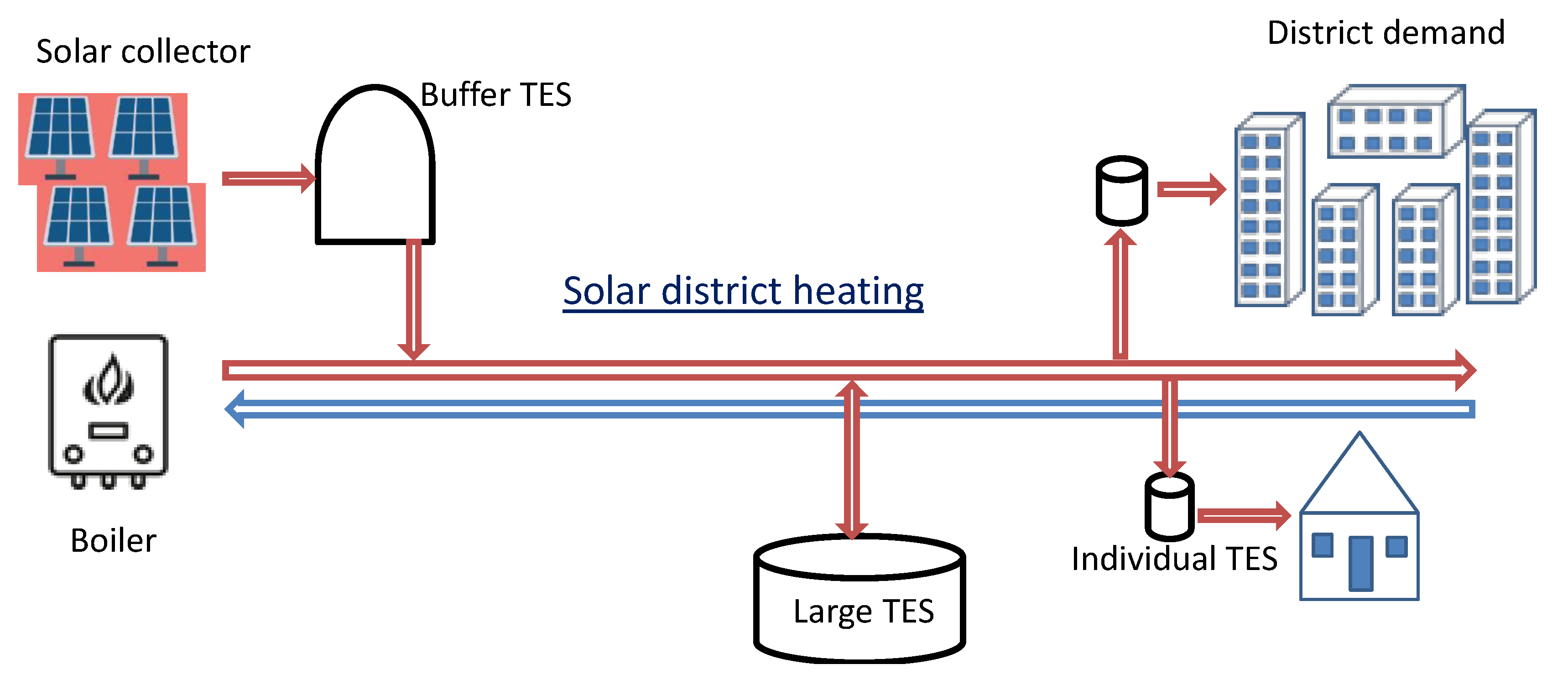
A DHN with high solar thermal penetration usually requires large scale storages [29,30] in the main network. Complementary smaller baffle storages close to each end user can be employed to smooth load fluctuation. In some cases where a heating connection is unavailable, movable TES can be employed [23,31] from a RRES production to the main DHN. In case of local space limitation, indirect PCM TES is generally preferable than sensible heat storage thanks to their high specific storage capacity [28,32]. Illustrated in Figure 2 are possible TES systems integrated to a low-grade heat recovery network.
Particularly in a solar district heating network, a well dimensioned central TES system could optimize energy use. A well dimensioned thermal energy storage allows optimal capacity sizing for solar collectors. Moreover, compared with configurations without TES, the one with a buffer TES has much longer working hour for the solar collector. This means less primary energy consumption from boilers [33].
In terms of temperature, storage systems with low-temperature (<100 °C) could be potentially applied to future centralised or decentralised heating networks. Especially after pressurized water or steam heating disappear, the storage with hot water or PCM becomes easier. Very low temperature TES with storage temperature below 70 °C are expected to be extensively applied to modern energy networks.
2.2. Main Technical Characteristics of TES Systems
For all the above-mentioned TES systems, the following characteristics are relevant for application: (i) energy storage capacity, ; (ii) storage time; (iii) charging and discharging rate, and ; and (iv) storage efficiency, .
Among these parameters, the energy storage capacity is the most dominant one. For a sensible TES system, its capacity can be directly obtained by multiplying the storage volume , heat storage medium density and its heat capacity . In the case of indirect TES using PCM, the storage capacity is comprised of the enthalpy change during phase change process, in addition to the sensible energy storage. With the same storage volume, a PCM based indirect storage system usually holds higher energy capacity. In other words, the same energy capacity requires smaller storage volume in the case of PCM.
Another important characteristic is the energy charging and discharging rate. For direct sensible TES, its charging and discharging rates are determined by pump flow rates and the storage temperature. For indirect TES such as systems incorporating PCM, their charging and discharging rates are mainly limited by the heat exchange rate between Heat Transfer Fluid (HTF) and storage medium (e.g., PCM). Shown in Equations (1) and (2) are expressions of charging rates for direct and indirect TES systems, respectively:
For direct TES systems such as tank storage or aquifer TES, its charging or discharging rates are limited only by pump circulation flow rate . For indirect systems such as PCM storage or BTES using soil as storage medium, the specific charging rate is closely influenced by the total heat exchange coefficient H as well as the inner heat transfer area surface between HTF and storage medium, .
Another parameter, the thermal storage efficiency, is defined as the ratio of useful, discharged energy and charged energy from/into a TES. (Equation (3)):
The fact of applying integral function to and is that the charging and discharging rates are highly time-dependent since they are subjected to demand/production fluctuations. Consequently, the storage time is unpredictable since the TES is not necessarily totally empty before the next charging starts. For an annual analysis, the integral should be done for 8760 h.
It worth noting that the energy loss of a TES system depends on its storage duration as well as the heat loss rate , as expressed by Equation (4):
where and are respectively storage medium temperature and ambient temperature. This expression remains applicable for both sensible and latent storage mechanisms.
Finally, the energy conservation rate during charging and discharging processes can be characterised by a dimensionless ratio (shown in Equation (4)). During the charging process, this ratio is expressed as effectively stored thermal power above surplus charging rate from the source side. The same ratio is applied to the discharging process. The ratio is always lower than 1 and it considers both energy losses during charging/discharging and the auxiliary power consumptions along with:
2.3. Scale Effect – the Importance of Thinking Big
For the case of sensible storage, high-capacity TES requires large storage volume, which in turn results in low energy loss through insulation. This could be explained from Equation (9), in which heat loss could be explained by thermal insulation UA number (heat loss coefficient) times the temperature difference between storage and ambient. Besides, the charged thermal energy for a sensible TES is determined by multiplying the density, the heat capacity of storage medium, the storage volume as well as the temperature difference between initial temperature (here supposed to be the same as ambient) and storage temperature. In the case of PCM-based TES, the heat capacity can be replaced by an effective capacity considering both liquid- and solid-phase specific heat and the phase-change enthalpy.
The specific energy loss, sometimes named thermal loss coefficient (s−1) [34], could be expressed by:
It is observed from Equation (9) that the specific energy loss rate is proportional to the ratio , representing the insulation surface area per unit of storage volume. Since this ratio decreases in cases of larger TES [35], it means lower specific energy loss rate for large-scale pit TES or ATES systems compared with small tank TES. This effect is often named scale effect.
In this study, hourly heat loss coefficient is considered as ranging from 0.9992 to 0.9997, corresponding to storage volumes ranging from 5 m3 to 100 m3. Determination of these values is based on assumptions of fully charged storage tanks with a height/diameter ratio h/d = 2, heat transfer coefficient U value of 0.28 W/(m−2·K−1), constant storage and ambient temperature values being respectively at 65 °C and 10 °C. Accumulated 7-day heat loss coefficient is 87% to 98% according to the storage volume since high volume storage is more efficient thanks to the abovementioned scale effect.
2.4. Heat Transfer Enhancement Necessity for Indirect TES
Since energy charging and discharging rates mean flexibility, it is desirable to have sufficiently adjustable values. The ratio of charging rate and storage capacity, named specific charging and discharging rate, , can be used to represent flexibility. The ratio is defined by Equation (10):
By examining the expressions of for direct and indirect TES systems through Equations (11) and (12), we find key influencing parameters on the flexibility issue: flow rate for direct systems and heat transfer rate for indirect ones:
For a direct TES system, the charging or discharging rate is limited only by pump circulation flow rate , which can be adjustable within the nominal limit by a varied-flowrate circulator. For indirect systems, the specific charging rate depends highly on the total heat exchange coefficient H as well as the inner heat transfer area surface between HTF and storage medium, . The {inner heat transfer area}/{storage volume} ratio directly influences the charging rate in a proportional manner. This requires heat transfer enhancement technologies such as optimisation in fluid contact between HTF and PCM, for example by direct contact configuration [23,31], or by maximising heat transfer coils [36], adding heat enhancement fins [37] or metal foam [38].
In summary, efficient TES systems are expected to hold high specific charging and discharging rate for flexibility convenience and low specific energy loss rate for better energy conservation. Both the two parameters are investigated in our model.
3. Simplified, Flux-Based Model towards a Rapid Estimation Tool
The TES model is part of our comprehensive waste heat mapping tool Recov’Heat. The simplified model includes production estimation, demand side identification as well as TES control by the energy flux towards or from the storage unit. Since the Recov’Heat tool is based on the exchange of data, i.e. energy/geography/distance/built surface/occupancy, the model should not include temperature nor flow rate details.
3.1. Recov’Heat Tool
An estimation tool covering major renewable and recovery heat sources and their characteristics may help decision makers evaluate its deployment in a district heating project. An annual estimation of diverse techno-economic indicators such as annual coverage rate, installation capacity, etc., should help decide whether a detailed study is necessary.
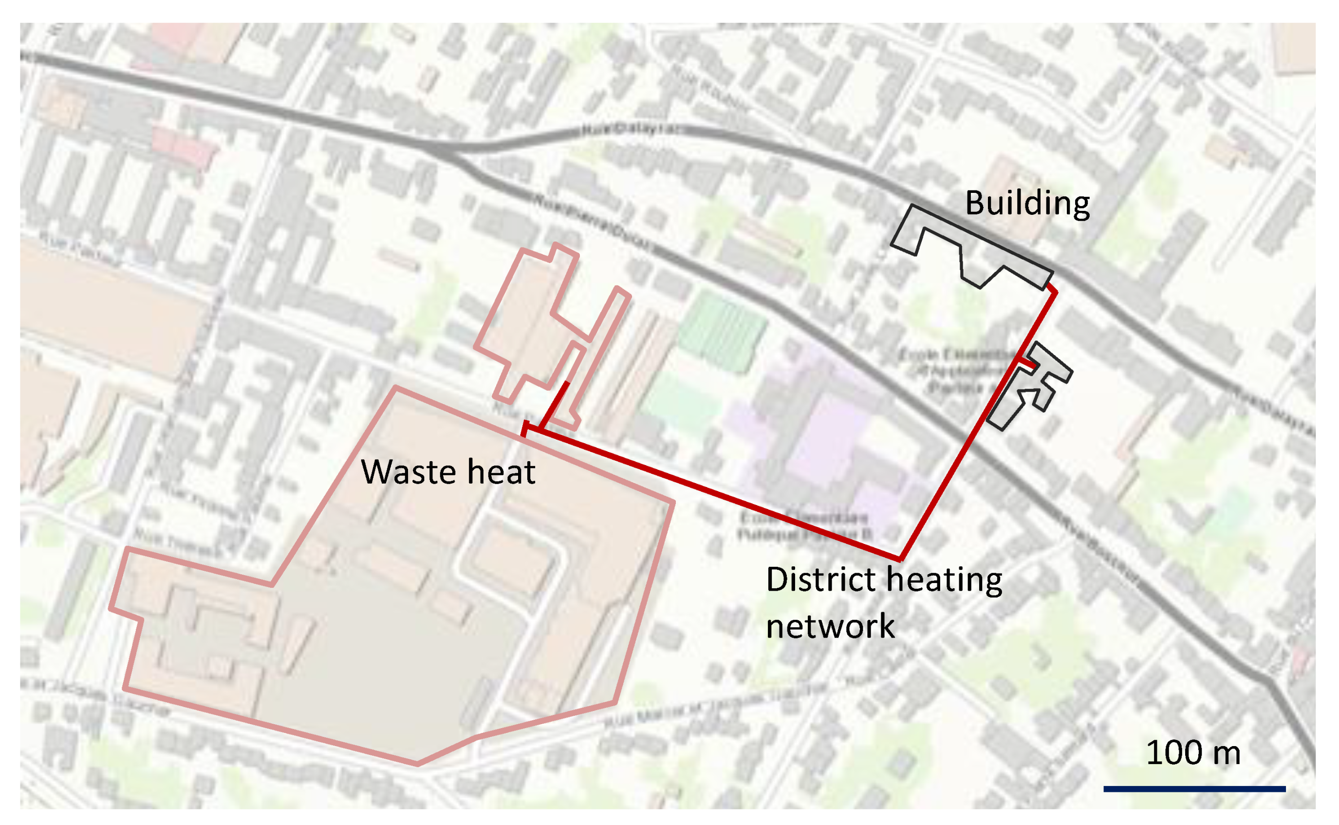
One of the aims of this easy-to-use, comprehensive estimation tool is to integrate into a Geographic Information System (GIS) tool (Figure 3) to accelerate the feasibility study of waste heat deployment by (i) visualizing the geographical and temporal distribution of waste heat in urban area, (ii) to estimate the heat demands from buildings and (iii) to evaluate the annual coverage rate. Potentially, the tool allows to visualize a DHN in terms of longer, density and tracing.
The TES model is one of the components of this comprehensive tool and as a result it cannot be based on detailed and tedious dynamic simulation. However, rigorous simulation is conducted to obtain data as inputs to the flux-based model.
3.2. Solar Thermal Production Potential
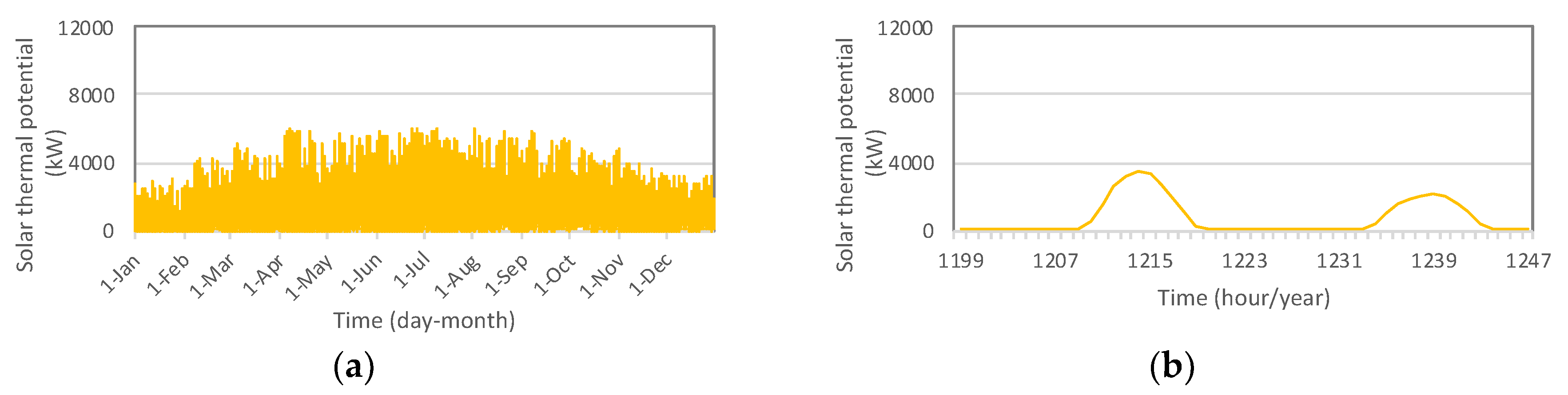
A large-scale solar thermal production with vacuum-tube collectors is simulated under the climate data of the Paris region in France. Since the solar conversion efficiency is dependent on the absorber temperature, which itself depends on the inlet HTF, we need to distinguish the direct and indirect TES. More specifically, during the charging process and compared with an indirect TES, water-based direct TES requires lower temperature difference between the source and the TES. Consequently, the temperature inlet into the solar absorber is higher in the case of indirect TES than the direct one. By estimating a temperature gap of 10 °C between the two cases, a decrease of 20% of the conversion efficiency can be estimated, i.e., 0.6 for the direct one and 0.48 for the indirect one. As a result, the required installation solar collector measures respectively 16,000 m2 and 20,000 m2 for the direct and indirect systems. Both suppose an orientation to the south and an inclination angle of 30°. The annual production curve is estimated simply by multiplying this efficiency with hourly solar radiation data obtained from Meteonorm embedded to TRNSYS [39]. It has to be noted that, to make comparison easier, the above parameters result in the same solar production for both cases. The estimation is based on statistical data in Paris region and the dynamic morning start-up time is not considered. The expected specific solar thermal production per year is 673 kWh/m2. Annual and 2-days’ curve variations of this source are shown in Figure 4a,b.
For all the four sources, their individual annual productions are very close: from 10,671 MWh to 10,878 MWh. These values correspond to an ideal share of 74.0% to 75.5% of the total annual demand which is explained in the following section.
3.3. Thermal Demand
As a highly behaviour-related consumption, the DHW demand profile down to hourly time step is considered [20,40]. The data is obtained by on-site measurement to residential applications. The total daily hot water demand is estimated to be 115 m3 per day, equivalent to an average draw-off of 144 L per day per family. Due to seasonal variation of mains water temperature, the DHW thermal demand is slightly higher in winter than in summer.
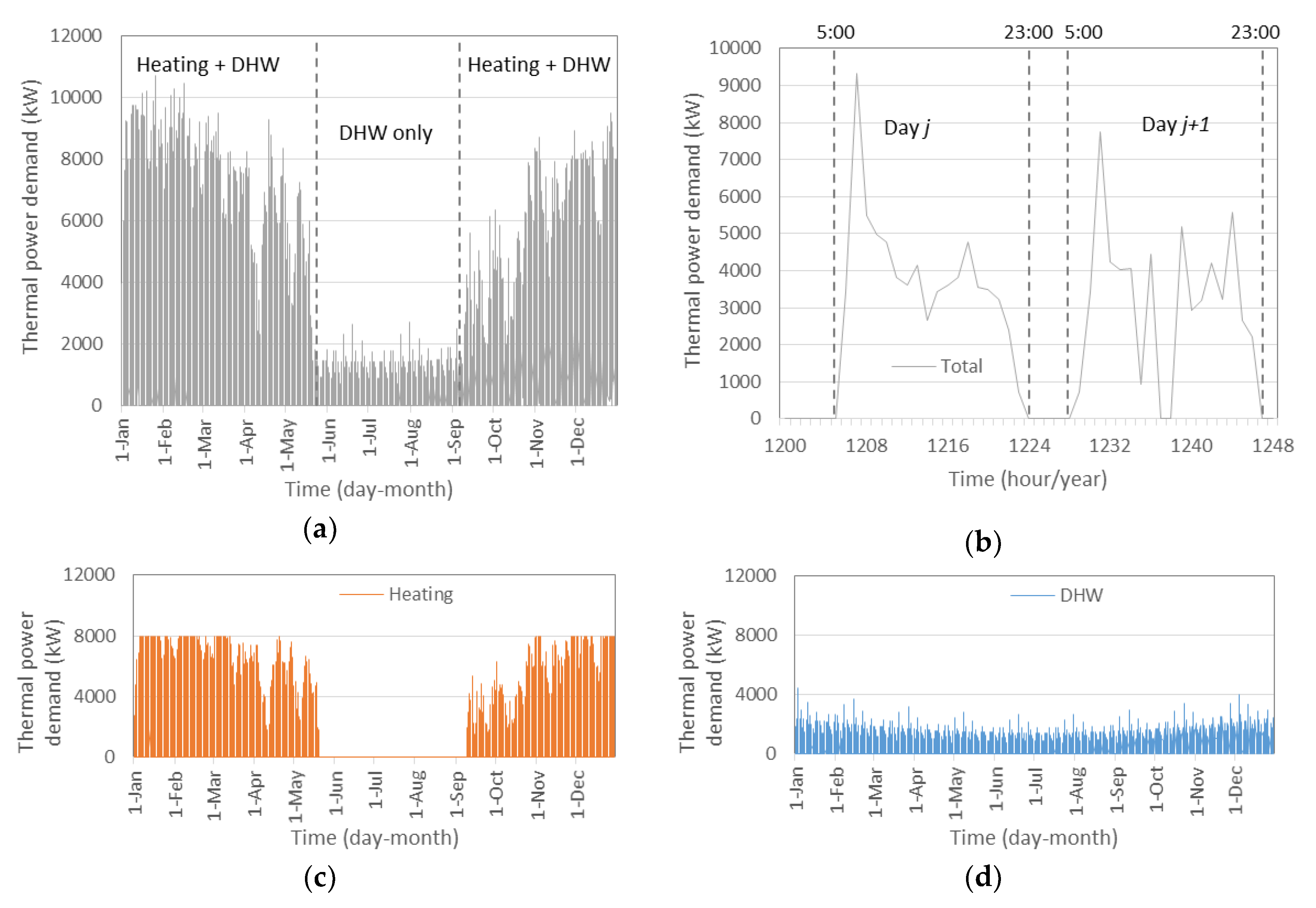
Annual demand profiles of the investigated total energy consumption, DHW-only, and heating-only demands are shown in Figure 5. To reflect the daily dynamic characteristic, a two days’ total consumption is also included. In terms of heating power, the peak demand is 10,686 kW in February, as shown in Figure 5a. This is mainly due to space heating during very cold period. On a daily basis, as shown in Figure 5b, energy demand takes place mainly between 5:00 to 23:00 during heating season. The heating supply is systematically cut during night hours, supposing that building inertia can keep a comfortable indoor environment from 23:00 to 5:00 next morning. In general, daily peak demand appears in the morning around 7:00 when both DHW and space heating run at their high loads.
The aggregated annual heat demand is 14,416 MWh, composed of a principal demand of 11,980 MWh from central heating and 2435 MWh for DHW supply. Since the original radiators are conserved during the building renovation, it is reasonable to maintain the feed temperature as that required by the radiators, i.e., at 70 °C. Consequently, some mixing is necessary for the DHW supply which requires 60 °C. This could result in some exergy destroy but only have marginal influence on the results due to the secondary characteristic of DHW consumption in the total demand. Therefore, both demands are directly primary thermal energy and they are supposed to require the same feed temperature.
3.4. Flux-Based Model
Although the potential benefits of TES in renewable district heating have been widely recognized [41], technology choice and storage sizing guidance are to be addressed in this work. Particularly, the comparison between water-based TES and PCM-based indirect one, regarding the charging/discharging limitation, may offer guidance on the proper choice of TES. A similar study in battery electricity storage is recently reported by Parra et al. [42]. In this study, batteries based on PbA and Li-ion technologies are compared in a photovoltaic (PV) power management application. The maximum charging current of the Li-ion battery is 15 times higher than that of PbA. Similar difference is implemented to the discharging rate. According to their comparison, Li-ion is the best solution for renewable power shifting when the PV fraction is higher than 50%. PbA battery, due to its lower charging rate, is more adapted to other applications such as DSM. Similarly, the above problematic also exists in thermal energy storage, namely between hot water based direct TES and PCM based indirect one. Our model considers these limitations.
In the model, simplifications are made to avoid constructing a detailed dynamic simulation program but to develop a rapid estimation tool to support decision making. Consequently, the model is based on pure energy flow with hourly time step. No flow rate, temperature or system control is considered in the current algorithm. Meanwhile, we do consider heat loss characteristic in TES. In this regard, the adopted methodology does not reflect the dynamic characteristics of the system such as flexibility, control strategy, which requires more detailed dynamic optimization shown in the literatures [41,43,44,45,46].
3.4.1. TES Parameters
For both direct and indirect TES, six storage capacities are investigated. The sizing criterion is based on the yearly maximum thermal demand, i.e., 10,686 kW. Applying ratios from 0.03 to 0.57 to the maximum thermal demand, we obtain six TES capacities. This indicates that under the peak load circumstance (i.e., peak cold weather conditions) and if the RRES production is zero, a fully charged TES could last several minutes (0.03 h) to about half an hour (0.57 h). However, in most of the time, the TES discharging is supposed to be capable to last more than this duration since the real load should be much lower than the peak one. In addition, a zero-storage case and ideal case are also presented. For the latter, the annual RRES potential is supposed to be entirely consumed by the clients (unlimited TES capacity and zero loss during charging/discharging/storage).
Physically, the above energy capacities (from 299 to 6091 kWh) match sensible TES volumes from 5 to 100 m3 of water (from 10 °C to 65 °C). To consider the stratification factor which could degrade the availability of water at relevant temperatures, a factor of 0.95 is used for over dimensioning the volume. Concerning indirect TES by PCM, the TES volume ranges from 4 to 75 m3 proportionally. This is thanks to the higher storage capacity by phase change enthalpy. In addition, to consider the volumes occupied by auxiliaries such as heat exchanger coils or tank envelop, the total gross TES volumes are estimated. We take a 10% extra volume for tank envelops for the direct water-based TES while 25% for indirect PCM-based ones since they also require heat exchangers (Table 1).
Minimum and maximum charging or discharging rates to/from a TES are defined as functions of TES type and capacity. The maximum charging and discharging rate for indirect TES is nearly ¼ of the direct one.
For direct TES, 2% of the TES capacity is taken as the minimum charging power and that of maximum value is 98% of the TES capacity. In other words, under the maximum charging rate, 0.98 h is needed to fully charge a storage system starting from empty. With the lowest charging rate, a TES turns fully charged within 50 h. The part of surplus over the maximum charging rate will be curtailed while that under the minimum rate will not be put in storage even if the TES is not fully charged. The above values remain applicable to the discharging process:
For indirect TES, their minimum and maximum charging rates are defined as 2% and 25% of the corresponding TES capacities. The maximum charging rate, considered as 25% of the capacity, is obtained from analyzing reported experimental results including inorganic paraffin or organic PCMs. For example, in the experimental results reported by Wang et al. [23], a charging rate of 2.287 kW has been observed for a 9.15 kWh storage corresponding to 74 kg PCM (the sugar alcohol erythritol). Thus, compared with direct storage, the lower maximum charging rate gives more limitation on indirect TES functionality due to inefficient heat exchange between HTF and storage medium. Some other researches show much better performance in terms of charging speed. In the study of Merlin et al. [47], a graphite doped paraffin composite is able to be charged in 0.06 h (6 kWh with a charging rate of 100 kW). But in most studies, the maximum charging rate is much lower than this value and we decided to keep the value of 25%, i.e., a minimum charging time of 4 h, as the maximum charging rate limitation in the case of indirect TES:
The energy conservation rates during charging and discharging processes, considering both heat losses and auxiliary power consumption, are assumed to be . This value remains the same for both direct and indirect systems. It worth noting that the energy conservation rate is also related to the minimum charging or discharging limitation. A ratio of 0.02 is used to determine the minimum charging or discharging limitation, and it represents the part of energy loss due to heat dissipation and auxiliary equipment consumption. This is equivalent to the value of 0.98 for energy conservation rate. The above TES parameters are summarized in Table 1.
3.4.2. Model Flowchart
The main inputs to the model are pre-identified hourly energy demands and solar production during a year (8760 h). All TES characteristics, e.g., the range of sizing, type (direct or indirect) and associated charging/discharging constraints, are integrated in the model. Output parameters include annual solar fraction, solar recovery rate, etc.
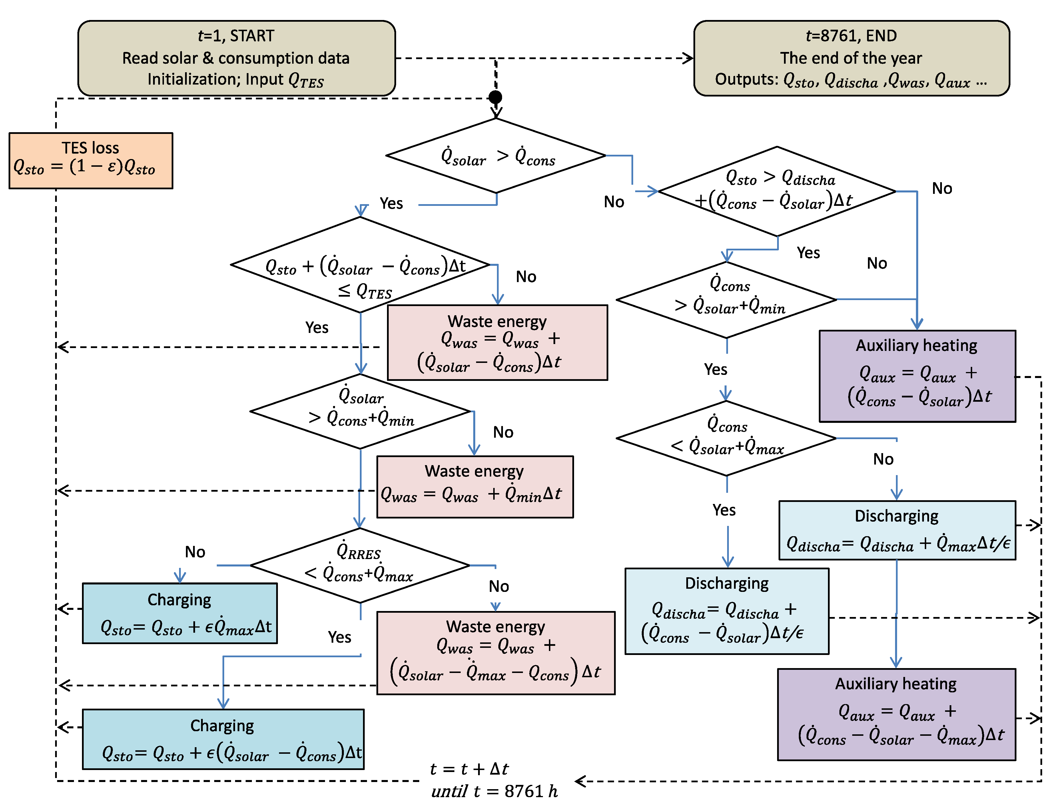
The program, running at a time step of 1 h in the Matlab® [48] environment (The MathWorks, Inc., Massachusetts 01760 USA), is described in Figure 6. For each time step, it starts by comparing solar production and heat demand. If surplus production is expected, it checks each of the three conditions: (i) does TES have extra space for charging?; (ii) is the charging rate higher than the minimum charging rate limited by the TES capacity? and (iii) is the charging rate lower than the maximum charging rate which is also linked to the TES capacity? If all above conditions are satisfied, the instantaneous surplus energy is charged into the TES. Otherwise, a part or the entire surplus becomes waste energy (identified as capacity limited, Pmin limited or Pmax limited losses). These losses are recorded for further evaluation.
On the contrary, when the potential production is lower than the demand, the program checks the following criteria: (i) is TES fully/partially charged? (ii) is the discharging need is higher than the Pmin limitation? and (iii) is the discharging need is lower than Pmax limitation? A discharge will be actuated under all the above limitations. If necessary, the program uses a gas boiler to satisfy the complementary load. For boiler heat supply when the solar production is insufficient, its performance efficiency is assumed to be 98%. This value is reasonable especially in the case of large capacity condensing gas boilers.
3.5. Evaluation Criteria
Evaluation indicators are considered both from the point of view of solar thermal exploitation and regarding the TES itself. First of all, from the client or primary energy consumption point of view, the solar fraction gives important information on techno-economic feasibility of a project. This fraction (also known as solar coverage rate), fsolar, is defined as the total annual renewable/recovery energy within the total demand. This value may vary according the size of TES and it is represented by fsolar,0 for the case where no TES system is available. Additionally, the ideal part of solar in its total annual consumption, defined as fsolar,i, can provide the limit of exploration of studied solar thermal installation in terms of coverage rate. This ideal situation supposes that a capacity unlimited, zero loss TES is integrated in the system and it can shift the entire surplus production to later usages. Finally, from the TES investment point of view, State of Charge (SOC) is analysed. This is defined by the ratio of charged energy and the capacity. SOC gives information on how the TES is operated annually.
Definitions of all the above indicators are shown in Equations (19)–(21):
Another evaluation parameter, Recovery Rate (RR), is used to represent the effectively recovered energy above the total annual recoverable potential. This stands for the effective recovery rate of a studied source:
where represents the total annual solar potential, kWh. The three losses , and signify unrecovered energy due to one of the three reasons: (i) solar production is lower than the minimum storable value thus not stored, ; (ii) solar production is higher than the maximum charging value and the extra energy is cut, ; and (iii) the TES is charged to its full capacity and any extra production should be considered as curtailed energy, .
4. Results and Discussion
4.1. Solar Fraction and Recovery Rate
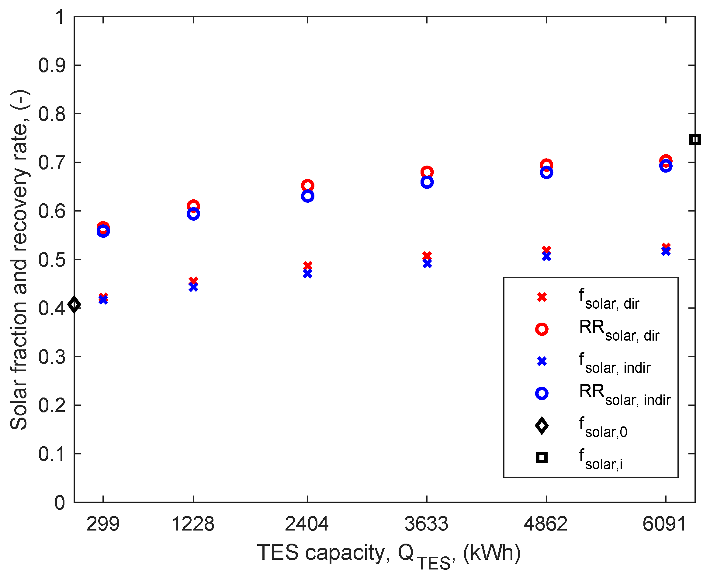
The solar fraction with different TES capacities is shown in Figure 7. A clear increase in solar fraction is observed with the integration of TES. We note that the ideal solar share is close to 75%, which is much higher than the shown real-case solar fractions in the figure. For example, with the studied TES capacities, the solar fraction fluctuates from 42% and 52%. Back to the no TES situation, the solar share is fsolar,0 = 41%. Following certain legislations, namely those requiring at least 50% of renewable injections, projects are only legible to benefit governmental aids if an appropriate TES system is planned.
Figure 7 also illustrates the variation of recovery rate (RR) as a function of TES capacities. This parameter is relative to the source side, and it gives information on how the renewable potential is exploited. It is shown, with investigated TES capacities, that solar thermal system can be deployed by only 56% to 70% of its total potential production. As explained, this is due to the high mismatching factor between this source and the heating-dominated demand.
Comparing direct TES with indirect ones, however, we surprisingly remark very little difference both in terms of solar fraction and in terms of recovery rate. As indicated in the modeling methodology, we adopt more strict discharging and charging power limitations to indirect TES, i.e., the charging and discharging power are only ¼ of an equivalent direct one. It is thus worthwhile to conduct a detailed, dynamic analysis for a time period.
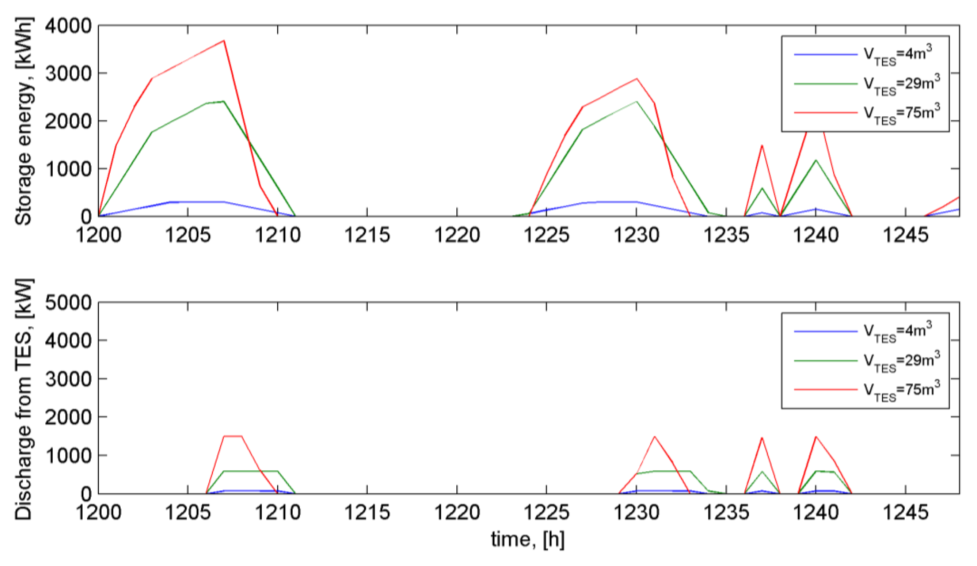
4.2. Direct or Indirect Storage?
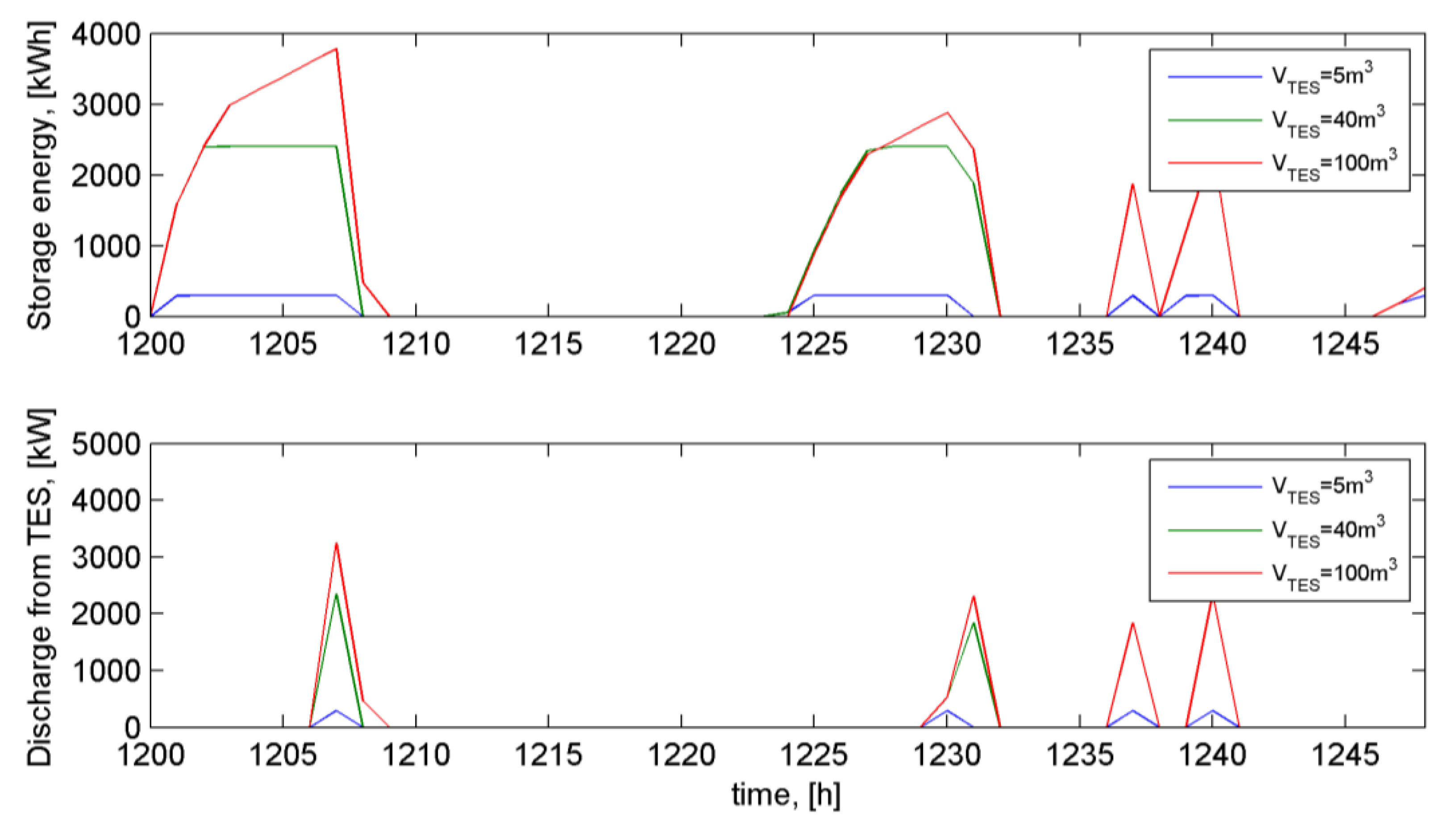
For direct and indirect TES, they are both alternatively charged and discharged but in different manner. In Figure 8 and Figure 9, we compare the stored energy and discharging power for direct TES and indirect ones, both holding the same storage capacity. The PCM indirect one gives more limitations to the charging and discharging rate. The analysis is based on a comparison between the case of TES capacities of 299, 3633 and 6091 kWh.
The little impact of storage medium, i.e., water or PCM, on the final solar fraction, can be explained by an auto-regulation characteristic of PCM. For the demand and solar production potential, the same dynamic curves are used during the period of 20–21 February. We observe that direct TES is soon fully charged while there is still surplus solar production (Figure 8). The charging of indirect TES, however, is self-regulated since it is more limited by its charging rate. As in Figure 9, the full capacity is only achieved during 2–3 h of charging, instead of only 1 h for the direct one. This way, the charging and discharging of indirect TES is less rapid but lasts longer. The result of this auto-regulation is the annual discharging energy of direct and indirect TES are nearly equivalent. In other words, the indirect TES has comparable performance as that of direct TES.
4.3. The Seasonal Variation of Storage Time
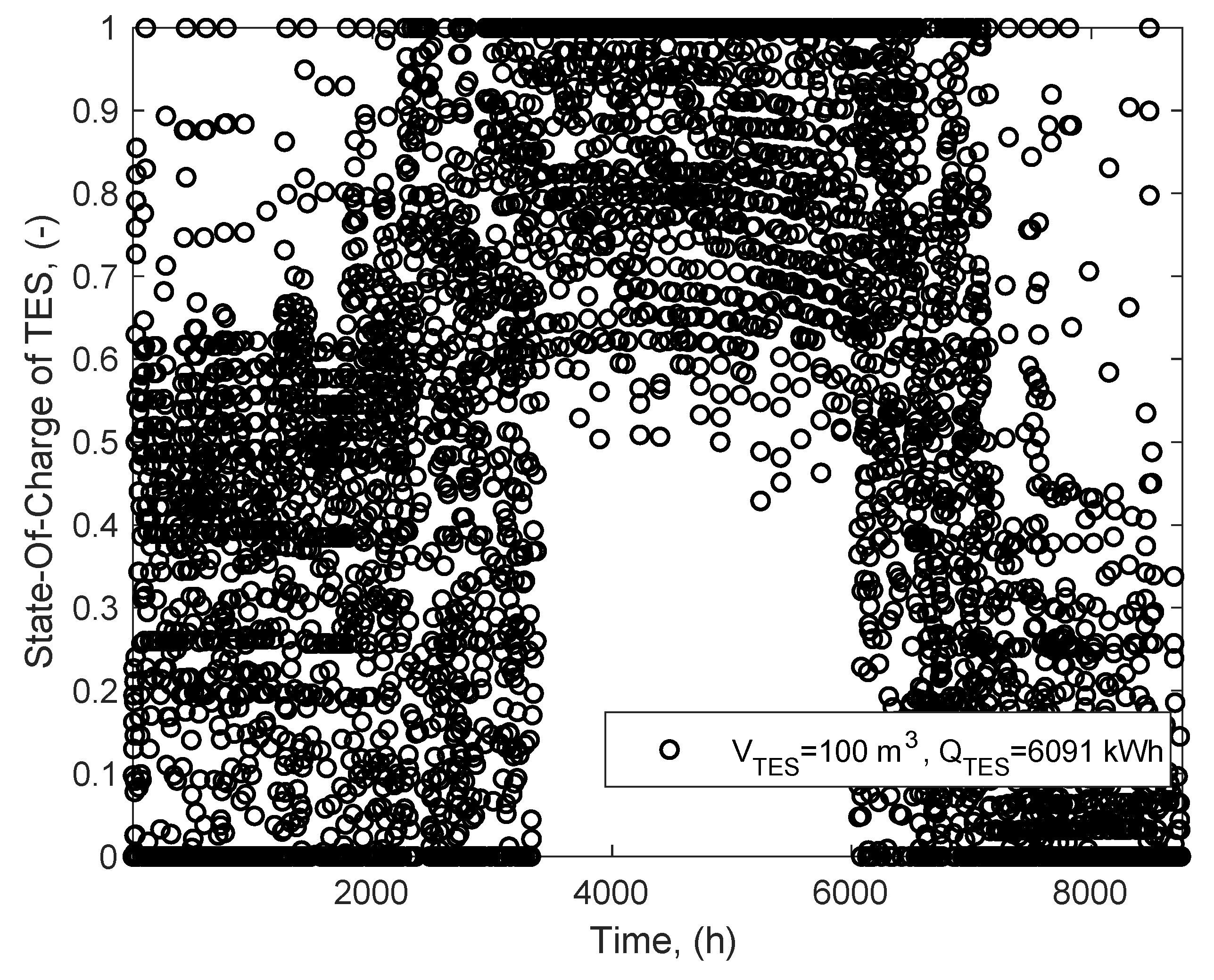
The storage time depends highly on the intermittent characteristics between the demand and the production. Shown in Figure 10 is the annual variation of the state of charge (SOC, 0–100%) of TES in a year. The result is based on a 100 m3 direct TES, corresponding to a storage capacity of 6091 kWh. The value of the SOC is clearly separated by heating seasons: between May (3600 h) and August (6000 h), the TES is always charged at higher than 45% of its full capacity. The TES is never fully discharged during this period, meaning no boiler operation is needed during this season. In cold seasons such as January and December, in contrary, the TES is rarely fully charged. Its SOC varies from 0 to 65%, with a significant concentration at 0 due to peak heating demand.
The 100 m3 TES plays a role of hourly storage other than seasonal shifting since otherwise the charging and discharging process would be more progressive.
4.4. Economic and Environmental Analyses
The economic-environmental assessment follows a simplified approach focusing on the TES itself. Only initial investment cost of TES is considered, and its value is taken as 1500 €/m3. No maintenance or other material costs (such as storage medium, i.e., water or PCM) are included. The analysis is based on a comparison between the case of no TES and that of 100 m3 hot water TES integration.
From an economic point of view, integrating a 100 m3 TES reduces the payback period for the solar thermal plant by 1 year. The estimation is supported by a payback calculation for three cases: (i) solar thermal without TES + auxiliary gas boiler, (ii) solar thermal with TES + auxiliary gas boiler, (iii) only gas boiler. For the initial investment in equipment, we suppose a price of 100 €/m2 for solar panels, and 160,000 € for gas boilers (including auxiliary). The initial investment is thus respectively 1.76 M€, 1.91 M€ and 0.16 M€ for the three cases. Then during the operation, as the solar share rises from 41% to 52% thanks to the TES unit, useful solar energy increases by 1701 MWh within the total demand (14,416 MWh). Considering 4% of auxiliary electricity consumption at a rate of 0.15 €/kWh and gas price of 0.05 €/kWh, the annual cost for the three cases is 460,735 €, 390,962 € and 720,800 €. This way, the case i) will have a payback period of 6.3 years on the basis of the case iii); while that of the case ii) is reduced to 5.2 years thanks to the use of renewable and the storage.
Environmental analysis uses GreenHouse Gas (GHG) emission as an indicator and it is significantly reduced thanks to TES. In France, GHG emission factors for electricity are estimated to be 0.055 t-eq CO2/MWh and 0.206 t-eq CO2/MWh for natural gas [49]. For the case of TES integration, the increased solar thermal utilization has only a price of 3.7 t-eq. CO2/year from its 4% auxiliary electricity consumption. In contrast, the case without TES must burn gas to compensate the mismatched solar production and that would result in an additional 350.4 t-eq. CO2/year.
5. Conclusions
In this study, we have developed a simplified decision-making tool for the integration of TES in a solar district heating. The emphases are both on the size issue of TES and the comparison between direct and indirect TES. Storage capacities from 299 to 6 091 kWh are analysed and they correspond to either 5 to 100 m3 direct hot water storage, or 4 to 75 m3 of indirect PCM storage. The hourly-based program is very convenient to use, and it only requires energy flux data from the demand and solar production sides. Economic-environmental evaluation can provide key information about the viability of a large-scale solar thermal project. The model provides useful messages for energy user (solar fraction, energy gain), energy service operators (TES size and SOC) and local communities/industries (solar energy recovery rate).
The integration of TES can help increase both solar fraction of the demand side and recovery rate of the sources. For example, with only integration of hot water tank of 100 m3, a solar heating project may see its solar share increase from 41% to 52%. The useful volume of this TES is only equivalent to a 36 m2 office with 2.8 m ceiling-high. Considering 800 households benefiting this carbon free energy, finding such a space should be reasonable. In addition, indirect TES based on PCM can economise 25% of storage volume (thus space occupation) while giving equivalent performances. This result provides arguments for those who research in the field of not only PCM-based indirect thermal energy storage, but also other indirect ones like borehole, soil, etc.
Our future works will be focused on the coupling of different waste energy sources in a dynamic district heating network. Installation of TES of different capacities both at the central production plant and/or at the end-users will be investigated. Another ongoing work is on the model sensibility regarding the storage temperature which is over simplified in the current version. Also, the heat transfer between HTF and PCM is only roughly considered, as well as the volume of heat transfer tubes which can occupy non-negligible volume compared with that of PCM.
Author Contributions
Conceptualization, methodology, software, validation, writing and editing, X.G.; resources, A.G.; validation and review, A.G. and C.W.; funding acquisition, X.G.
Funding
The current study received funding from the French Ministry of Europe and Foreign Affairs (MEAE), through the PHC Xu Guangqi program (N°: 41269UL, 2018).
Acknowledgments
Xiaofeng Guo would like to express his acknowledgement for the mobility funding from the French Ministry of Europe and Foreign Affairs (MEAE), within the Jeunes Talents France-Chine program, (N°: 925116B, 2018).
Conflicts of Interest
The authors declare no conflict of interest. The funders had no role in the design of the study; in the collection, analyses, or interpretation of data; in the writing of the manuscript, or in the decision to publish the results.
References
- European Commission. Proposal for a Directive of the European Parliament and of the Council Amending Directive 2010/31/EU on the Energy Performance of Buildings; European Commission: Brussels, Belgium, 2016. [Google Scholar]
- Lund, H.; Werner, S.; Wiltshire, R.; Svendsen, S.; Thorsen, J.E.; Hvelplund, F.; Mathiesen, B.V. 4th Generation District Heating (4GDH): Integrating smart thermal grids into future sustainable energy systems. Energy 2014, 68, 1–11. [Google Scholar] [CrossRef]
- Guo, X.; Hendel, M. Urban water networks as an alternative source for district heating and emergency heat-wave cooling. Energy 2018, 145, 79–87. [Google Scholar] [CrossRef]
- Reilly, A.; Kinnane, O. The impact of thermal mass on building energy consumption. Appl. Energy 2017, 198, 108–121. [Google Scholar] [CrossRef] [Green Version]
- Kensby, J.; Trüschel, A.; Dalenbäck, J.-O. Potential of residential buildings as thermal energy storage in district heating systems-Results from a pilot test. Appl. Energy 2015, 137, 773–781. [Google Scholar] [CrossRef]
- Ayón, X.; Gruber, J.K.; Hayes, B.P.; Usaola, J.; Prodanović, M. An optimal day-ahead load scheduling approach based on the flexibility of aggregate demands. Appl. Energy 2017, 198, 1–11. [Google Scholar] [CrossRef] [Green Version]
- Wang, C.; Guo, X.; Zhu, Y. Energy saving with Optic-Variable Wall for stable air temperature control. Energy 2019, 173, 38–47. [Google Scholar] [CrossRef]
- Gadd, H.; Werner, S. Achieving low return temperatures from district heating substations. Appl. Energy 2014, 136, 59–67. [Google Scholar] [CrossRef] [Green Version]
- Gadd, H.; Werner, S. Heat load patterns in district heating substations. Appl. Energy 2013, 108, 176–183. [Google Scholar] [CrossRef] [Green Version]
- Rezaie, B.; Rosen, M.A. District heating and cooling: Review of technology and potential enhancements. Appl. Energy 2012, 93, 2–10. [Google Scholar] [CrossRef]
- Aronsson, B.; Hellmer, S. Existing Legislative Support Assessments for DHC. Available online: https://www.euroheat.org/wp-content/uploads/2016/04/Ecoheat4EU_Existing_Legislative_Support_Assessments.pdf (accessed on 1 May 2019).
- ADEME L’Agence de l’environnement et de la maîtrise de l’énergie (ADEME). Available online: http://www.ademe.fr/ (accessed on 1 May 2019).
- Berthou, M.; Bory, D. Overview of waste heat in the industry in France. In Proceedings of the ECEEE, Giens, France, 3–8 June 2019; pp. 453–459. [Google Scholar]
- Chan, C.W.; Ling-Chin, J.; Roskilly, A.P. A review of chemical heat pumps, thermodynamic cycles and thermal energy storage technologies for low grade heat utilisation. Appl. Therm. Eng. 2013, 50, 1257–1273. [Google Scholar] [CrossRef]
- Law, R.; Harvey, A.; Reay, D. Opportunities for low-grade heat recovery in the UK food processing industry. Appl. Therm. Eng. 2013, 53, 188–196. [Google Scholar] [CrossRef]
- Deloitte, C. Energy market reform in Europe. Eur. Energy Clim. Polic. Achiev. Chall. 2020 2015, 19, 165. [Google Scholar]
- Brueckner, S.; Miro, L.; Cabeza, L.F.; Pehnt, M.; Laevemann, E. Methods to estimate the industrial waste heat potential of regions-A categorization and literature review. Renew. Sustain. Energy Rev. 2014, 38, 164–171. [Google Scholar] [CrossRef]
- Ammar, Y.; Joyce, S.; Norman, R.; Wang, Y.; Roskilly, A.P. Low grade thermal energy sources and uses from the process industry in the UK. Appl. Energy 2012, 89, 3–20. [Google Scholar] [CrossRef]
- EFFICACITY. Institute of Research and Development for Urbain Energy Transition. Available online: https://www.efficacity.com/ (accessed on 1 May 2019).
- Goumba, A.; Chiche, S.; Guo, X.; Colombert, M.; Bonneau, P. Recov’ Heat: An Estimation Tool of Urban Waste Heat Recovery Potential in Sustainable Cities. In Proceedings of the AIP Conference Proceedings, College Park, MD, USA, 23 February 2017; Volume 1814. [Google Scholar]
- EFFICACITY Recov’heat, estimation tool for urban waste heat recovery projects. Available online: http://tools.efficacity.com (accessed on 1 May 2019).
- IEA SHC, Task 45. Large Scale Solar Heating and Cooling Systems. Available online: http://task45.iea-shc.org (accessed on 1 January 2017).
- Wang, W.; Guo, S.; Li, H.; Yan, J.; Zhao, J.; Li, X.; Ding, J. Experimental study on the direct/indirect contact energy storage container in mobilized thermal energy system (M-TES). Appl. Energy 2014, 119, 181–189. [Google Scholar] [CrossRef]
- Fumey, B.; Weber, R.; Baldini, L. Liquid sorption heat storage-A proof of concept based on lab measurements with a novel spiral fined heat and mass exchanger design. Appl. Energy 2017, 200, 215–225. [Google Scholar] [CrossRef]
- Heizkörper, H.M. Thermal Battery-HM Heizkörper. Available online: http://www.hm-heizkoerper.de/en/thermal-battery (accessed on 15 June 2017).
- Sarbu, I.; Sebarchievici, C.; Sarbu, I.; Sebarchievici, C. A Comprehensive Review of Thermal Energy Storage. Sustainability 2018, 10, 191. [Google Scholar] [CrossRef]
- Cabeza, L.F.; Sole, C.; Castell, A.; Oro, E.; Gil, A. Review of Solar Thermal Storage Techniques and Associated Heat Transfer Technologies. Proc. IEEE 2012, 100, 525–538. [Google Scholar] [CrossRef]
- Guo, X.; Goumba, A.P.; Rocaries, F.; Bourouina, T.; Zhao, D.; Zhao, J.; Deng, S. Process Intensification technologies applied to Thermal Energy Storage–Principles, successful applications and perspectives. In Proceedings of the SDH2015, 3rd International on Solar District Heating Conference, Toulouse, France, 26–31 October 2015. [Google Scholar]
- Schmidt, R.; Fevrier, N.; Dumas, P. Key to Innovation Integrated Solution: Smart tHermal Grids. Smart Cities Stakeholder Platform. Available online: https://eu-smartcities.eu/sites/default/files/2017-10/Smart%20Grid%20Systems%20-%20Smart%20Cities%20Stakeholder%20Platform%20%281%29_0.pdf (accessed on 1 May 2019).
- Wang, H.; Yin, W.; Abdollahi, E.; Lahdelma, R.; Jiao, W. Modelling and optimization of CHP based district heating system with renewable energy production and energy storage. Appl. Energy 2015, 159, 401–421. [Google Scholar] [CrossRef]
- Guo, S.; Li, H.; Zhao, J.; Li, X.; Yan, J. Numerical simulation study on optimizing charging process of the direct contact mobilized thermal energy storage. Appl. Energy 2013, 112, 1416–1423. [Google Scholar] [CrossRef]
- Guo, X.; Goumba, A.P. Process Intensification Principles Applied to Thermal Energy Storage Systems-A Brief Review. Front. Energy Res. 2018, 6, 17. [Google Scholar] [CrossRef]
- Verda, V.; Colella, F. Primary energy savings through thermal storage in district heating networks. Energy 2011, 36, 4278–4286. [Google Scholar] [CrossRef]
- Buoro, D.; Pinamonti, P.; Reini, M. Optimization of a Distributed Cogeneration System with solar district heating. Appl. Energy 2014, 124, 298–308. [Google Scholar] [CrossRef]
- Hadorn, J.-C. Storage Solutions for Solar Thermal Energy Reason 1: Time! Available online: http://www.viking-house.ie/downloads/Long%20Term%20Heat%20Stores,%20Swiss%20Study.pdf (accessed on 1 May 2019).
- Castell, A.; Belusko, M.; Bruno, F.; Cabeza, L.F. Maximisation of heat transfer in a coil in tank PCM cold storage system. Appl. Energy 2011, 88, 4120–4127. [Google Scholar] [CrossRef]
- Ma, Z.; Yang, W.-W.; Yuan, F.; Jin, B.; He, Y.-L. Investigation on the thermal performance of a high-temperature latent heat storage system. Appl. Therm. Eng. 2017, 122, 579–592. [Google Scholar] [CrossRef]
- Yang, J.; Yang, L.; Xu, C.; Du, X. Experimental study on enhancement of thermal energy storage with phase-change material. Appl. Energy 2016, 169, 164–176. [Google Scholar] [CrossRef]
- CSTB Meteonorm, TRNSYS Package. Available online: http://logiciels.cstb.fr/Thermique-METEONORM 2012 (accessed on 1 May 2019).
- Guo, X.; Goumba, A.P. Air source heat pump for domestic hot water supply: Performance comparison between individual and building scale installations. Energy 2018, 164, 794–802. [Google Scholar] [CrossRef]
- Powell, K.M.; Kim, J.S.; Cole, W.J.; Kapoor, K.; Mojica, J.L.; Hedengren, J.D.; Edgar, T.F. Thermal energy storage to minimize cost and improve efficiency of a polygeneration district energy system in a real-time electricity market. Energy 2016, 113, 52–63. [Google Scholar] [CrossRef]
- Parra, D.; Norman, S.A.; Walker, G.S.; Gillott, M. Optimum community energy storage for renewable energy and demand load management. Appl. Energy 2017, 200, 358–369. [Google Scholar] [CrossRef]
- Blackburn, L.; Young, A.; Rogers, P.; Hedengren, J.; Powell, K. Dynamic optimization of a district energy system with storage using a novel mixed-integer quadratic programming algorithm. Optim. Eng. 2019, 20, 1–29. [Google Scholar] [CrossRef]
- Powell, K.M.; Edgar, T.F. Modeling and control of a solar thermal power plant with thermal energy storage. Chem. Eng. Sci. 2012, 71, 138–145. [Google Scholar] [CrossRef]
- Cole, W.J.; Powell, K.M.; Edgar, T.F. Optimization and advanced control of thermal energy storage systems. Rev. Chem. Eng. 2012, 28, 81–99. [Google Scholar] [CrossRef]
- Ellingwood, K.; Safdarnejad, S.; Rashid, K.; Powell, K.; Ellingwood, K.; Safdarnejad, S.M.; Rashid, K.; Powell, K. Leveraging Energy Storage in a Solar-Tower and Combined Cycle Hybrid Power Plant. Energies 2018, 12, 40. [Google Scholar] [CrossRef]
- Merlin, K.; Delaunay, D.; Soto, J.; Traonvouez, L. Heat transfer enhancement in latent heat thermal storage systems: Comparative study of different solutions and thermal contact investigation between the exchanger and the PCM. Appl. Energy 2016, 166, 107–116. [Google Scholar] [CrossRef]
- MathWorks MATLAB. MATLAB R2018b; The MathWorks: Natick, MA, USA, 2018. [Google Scholar]
- Seck, G.S.; Guerassimoff, G.; Maïzi, N. Heat recovery using heat pumps in non-energy intensive industry: Are Energy Saving Certificates a solution for the food and drink industry in France? Appl. Energy 2015, 156, 374–389. [Google Scholar] [CrossRef]
Figure 1.
Estimation of waste energy recovery potentials with a simplified TES model.

Figure 2.
Different thermal energy storage system in a solar district heating.

Figure 3.
Example of the application of waste heat recovery evaluation.

Figure 4.
Yearly and daily production potential curves of a 16,000 m2 solar thermal installation, (a) potential curve all through a year; (b) 48 h-based potential curve, 20–21 February, midnight to midnight.
Figure 4.
Yearly and daily production potential curves of a 16,000 m2 solar thermal installation, (a) potential curve all through a year; (b) 48 h-based potential curve, 20–21 February, midnight to midnight.

Figure 5.
Thermal energy demands for 800 residential apartments under the climate of Paris, (a) aggregated thermal demand, annual curve; (b) total thermal demand for two days of 21–22 February; (c) annual heating requirements and (d) annual DHW thermal demand.
Figure 5.
Thermal energy demands for 800 residential apartments under the climate of Paris, (a) aggregated thermal demand, annual curve; (b) total thermal demand for two days of 21–22 February; (c) annual heating requirements and (d) annual DHW thermal demand.

Figure 6.
General flowchart of the flux-based model.

Figure 7.
Solar fraction with different TES capacities and different TES types.

Figure 8.
Storage and discharging cycles in two days, direct hot-water based TES.

Figure 9.
Storage and discharging cycles in two days, indirect PCM based TES.

Figure 10.
Annual variation of the state-of-charge (SOC) of a 100 m3 direct TES used in a solar district heating. Out of the heating season and for 4 months, the 100 m3 TES is always charged between 40% of its total capacity and the full state. During heating seasons, however, the SOC fluctuates between 0 and 40–60% with a high distribution near zero.


Table 1.
Main characteristics of direct and indirect TES systems.
| Types | Total Volume (m3) | Medium | Storage Temperature (°C) | |||||
|---|---|---|---|---|---|---|---|---|
| Direct | 5 | 5.5 | 299 | Water | [10, 65] | 0.98 | 0.02 | 0.98 |
| 20 | 22 | 1228 | ||||||
| 40 | 44 | 2404 | ||||||
| 60 | 66 | 3633 | ||||||
| 80 | 88 | 4862 | ||||||
| 100 | 110 | 6091 | ||||||
| Indirect | 4 | 5 | 299 | PCM | 0.25 | 0.02 | 0.98 | |
| 15 | 19 | 1228 | ||||||
| 29 | 36 | 2404 | ||||||
| 45 | 56 | 3633 | ||||||
| 60 | 75 | 4862 | ||||||
| 75 | 94 | 6091 |
© 2019 by the authors. Licensee MDPI, Basel, Switzerland. This article is an open access article distributed under the terms and conditions of the Creative Commons Attribution (CC BY) license (http://creativecommons.org/licenses/by/4.0/).
Share and Cite
MDPI and ACS Style
Guo, X.; Goumba, A.P.; Wang, C. Comparison of Direct and Indirect Active Thermal Energy Storage Strategies for Large-Scale Solar Heating Systems. Energies 2019, 12, 1948. https://doi.org/10.3390/en12101948
AMA Style
Guo X, Goumba AP, Wang C. Comparison of Direct and Indirect Active Thermal Energy Storage Strategies for Large-Scale Solar Heating Systems. Energies. 2019; 12(10):1948. https://doi.org/10.3390/en12101948
Chicago/Turabian StyleGuo, Xiaofeng, Alain Pascal Goumba, and Cheng Wang. 2019. "Comparison of Direct and Indirect Active Thermal Energy Storage Strategies for Large-Scale Solar Heating Systems" Energies 12, no. 10: 1948. https://doi.org/10.3390/en12101948
Note that from the first issue of 2016, this journal uses article numbers instead of page numbers. See further details here.