Mixed Kernel Function Support Vector Regression with Genetic Algorithm for Forecasting Dissolved Gas Content in Power Transformers

Abstract

Forecasting dissolved gas content in power transformers plays a significant role in detecting incipient faults and maintaining the safety of the power system. Though various forecasting models have been developed, there is still room to further improve prediction performance. In this paper, a new forecasting model is proposed by combining mixed kernel function-based support vector regression (MKF-SVR) and genetic algorithm (GA). First, forecasting performance of SVR models constructed with a single kernel are compared, and then Gaussian kernel and polynomial kernel are retained due to better learning and prediction ability. Next, a mixed kernel, which integrates a Gaussian kernel with a polynomial kernel, is used to establish a SVR-based forecasting model. Genetic algorithm (GA) and leave-one-out cross validation are employed to determine the free parameters of MKF-SVR, while mean absolute percentage error (MAPE) and squared correlation coefficient (r²) are applied to assess the quality of the parameters. The proposed model is implemented on a practical dissolved gas dataset and promising results are obtained. Finally, the forecasting performance of the proposed model is compared with three other approaches, including RBFNN, GRNN and GM. The experimental and comparison results demonstrate that the proposed model outperforms other popular models in terms of forecasting accuracy and fitting capability.

1. Introduction

Power transformers is some of the most vital and expensive devices in power grids. They play a significant role in transferring energy and converting voltages to different levels. Any unexpected malfunction or failure of a power transformer may jeopardize the continuity of the power supply, cause catastrophic damages to electrical equipment and power system, and bring economic losses for power utilities and society. Therefore, considerable efforts have been made to detect and monitor the operating conditions of power transformers to keep transformers working under safe conditions [1,2,3].

Due to thermal stresses, electrical stresses and aging, the insulation systems (i.e., mineral oil, cellulose and solid insulation) of power transformers inevitably deteriorate and decompose. As a result, several kinds of gases are produced and dissolve in the mineral oil during the degradation process. Numerous approaches and models based on dissolved gas concentration and gas characteristics have been developed and utilized for the last decades [4,5,6,7]. The dissolved gas analysis (DGA) technique, a simple and effective method, has been widely applied to interpret the working conditions and incipient faults of power transformers. Key gases, including hydrogen (H₂), methane (CH₄), acetylene (C₂H₂), ethylene (C₂H₄) and ethane (C₂H₆), are commonly used by DGA methods to interpret working conditions and identify potential faults in power transformers [8,9]. Consequently, if the concentration of dissolved gas can be forecast exactly with historical data, incipient faults and their development trends can be determined in advance to implement corresponding maintenance plans and minimize latent losses.

Many approaches based on artificial intelligence (AI) have been proposed and applied for forecasting the concentration of dissolved gases in power transformers, such as grey model (GM) [10], artificial neural networks (ANN) [11,12,13,14,15], least squares support vector machine (LSSVM) [16,17,18,19] and support vector regression (SVR) [20,21], etc. Each approach has its own advantages and disadvantages. ANN methods, including back propagation neural network (BPNN), radial basis function neural network (RBFNN) and generalized regression neural network (GRNN), have superior self-learning, acceptable generalization, non-linear data handling capability. However, accurate forecasting of dissolved gases in power transformers requires massive amounts of historical data, which is infeasible in practice. Besides, the structure and related parameters of ANN need to be set properly to ensure satisfactory performance. These requirements mentioned above have restricted the application of ANN in the field of forecasting. The grey model method is capable of providing desirable forecasting result with small-scale data and has been used to predict dissolved gas concentrations in power transformers. However, grey models are only suitable to depict cases where the observed variables change monotonously with time like exponential laws. In practice, the variation of dissolved gas content in power transformers doesn’t follow the premise mentioned above owing to external factors. Thus, an inherent error will always exist when GM is adopted to forecast dissolved gas content in power transformers. Support vector regression (SVR) is regarded as an extended version of the support vector machine method and has received increasing attention in function estimation. SVR is established on the principle of structural risk minimization instead of empirical risk minimization, which makes it have a simpler structure, higher forecasting accuracy and better generalization performance [22].

In general, forecasting of dissolved gas content of power transformers is a non-linear time series problem. As one of the most important component of SVR, kernel functions convert non-linear and inseparable problems into linear divisible ones. Mixed-kernel functions (MKF) have recently attracted great attention since they are able to achieve better classification and regression performance [23,24]. According to literature reviews [10,11,12,13,14,15,16,17,18,19,20,21,22], previously proposed forecasting models are implemented by a single kernel, and MKF-SVR model for dissolved gas content forecasting is rarely investigated. Therefore, in this paper we intend to propose a novel forecasting model based on MKF-SVR to improve prediction performance. In addition, genetic algorithm (GA) is also applied to tune the parameters of MKF-SVR to further improve the forecasting performance.

The remainder of this paper is organized as follows: the methodology of MKF-SVR and GA is introduced in Section 2; Section 3 describes the main process of the proposed approach. The forecasting performance of the proposed approach is presented in Section 4. Finally, the conclusions are drawn in Section 5.

2. Methodology

2.1. Support Vector Regression

The support vector machine (SVM) method, first proposed by Vapnik in the 1990s, has been acknowledged worldwide as an effective and significant method for classification and regression. The subdivision of SVM that tackles the regression problem and function estimation is known as support vector regression (SVR). SVR has been applied in many different fields and obtained remarkable progress due to its advantages of simple structure and convenient application [25,26,27,28,29]. Compared with other AI approaches, the computational complexity of SVR is determined by the number of the support vectors instead of the dimensions of input data, which not only prevents the “dimension curse”, but also reduces computational cost.

Given a dataset $D=\left\{\left(x_i,y_i\right)\right\},(x_i\in R^n,y_i\in R,i=1,2,\cdots n)$, where x is the n-dimensional input variable and y is the corresponding output value. n represents the number of samples. A linear problem can be described by the function shown below:

$$f\left(x\right)=\langle \omega ,x\rangle +b$$

(1)

where $\omega$ and b denote weight coefficient and constant coefficient, respectively; $f\left(x\right)$ is the forecasting value. When it comes to a non-linear problem, kernel function $\phi \left(x\right)$ is applied to transform the low-dimension nonlinear problem to a high-dimension linear problem. The regression function is shown as Equation (2):

$$f\left(x\right)=\langle \omega ,\phi \left(x\right)\rangle +b$$

(2)

The parameters $\omega$ and b can be estimated by minimizing the regularized risk function:

$$\begin{array}{l}\min \frac{1}{2}{\Vert \omega \Vert }^2+\frac{C}{n}{\displaystyle \sum _{i=1}^n\epsilon \left(y_i-f\left(x_i\right)\right)}\\ s.t.\epsilon \left(y_i-f\left(x_i\right)\right)=\{\begin{array}{ll}0& \left|y_i-f\left(x\right)\right|\le \epsilon \\ \left|y_i-f\left(x\right)\right|-\epsilon ,& otherwise\end{array}\end{array}$$

(3)

where C is the penalty factor, which is used to balance empirical risk and confidence degree. $\epsilon (\cdot )$ denotes the $\epsilon$ -non sensitive loss function and $\epsilon$ represents for the $\epsilon$ -intensive loss parameter. Two non-negative slack variable ${\xi }_i$ and ${\xi }_i^{\ast }$ are introduced to facilitate the solving process and then the optimization problem becomes:

$$\begin{array}{l}\underset{\omega ,\xi ,{\xi }^{\ast }}{\min }\frac{1}{2}{\Vert \omega \Vert }^2+C{\displaystyle \sum _{i=1}^n\left({\xi }_i+{\xi }_i^{\ast }\right)}\\ s.t.\{\begin{array}{l}\langle \omega ,\phi \left(x\right)\rangle +b-y_i\le \epsilon +{\xi }_i\\ y_i-\langle \omega ,\phi \left(x\right)\rangle -b\le \epsilon +{\xi }_i^{\ast }& i=1,2,\cdots ,n\\ {\xi }_i,{\xi }_i^{\ast }\ge 0\end{array}\end{array}$$

(4)

Lagrangian multipliers are introduced to convert the problem described above to a dual optimization problem, which is shown as Equation (5):

$$\begin{array}{l}\min \frac{1}{2}{\displaystyle \sum _{i,j=1}^n\left({\alpha }_i^{\ast }-{\alpha }_i\right)\left({\alpha }_j^{\ast }-{\alpha }_j\right)K\left(x_i\cdot x_j\right)}+\epsilon {\displaystyle \sum _{i=1}^n\left({\alpha }_i^{\ast }+{\alpha }_i\right)}-{\displaystyle \sum _{i=1}^n{y}_i\left({\alpha }_i^{\ast }-{\alpha }_i\right)}\\ s.t.\{\begin{array}{ll}{\displaystyle \sum _{i=1}^l\left({\alpha }_i^{\ast }-{\alpha }_i\right)}=0& i=1,2,\cdots n\\ 0\le {\alpha }_i^{\ast },{\alpha }_i\le C\end{array}\end{array}$$

(5)

where ${\alpha }_i$ and ${\alpha }_i^{\ast }$ are the Lagrangian multipliers, $K\left(x_i\cdot x_j\right)$ is kernel function. Then, the support vector regression function $f\left(x\right)$ can be obtained as follows:

$$f\left(x\right)={\displaystyle \sum _{i=1}^n\left({\alpha }_i-{\alpha }_i^{\ast }\right)K\left(x_i,x\right)+b}$$

(6)

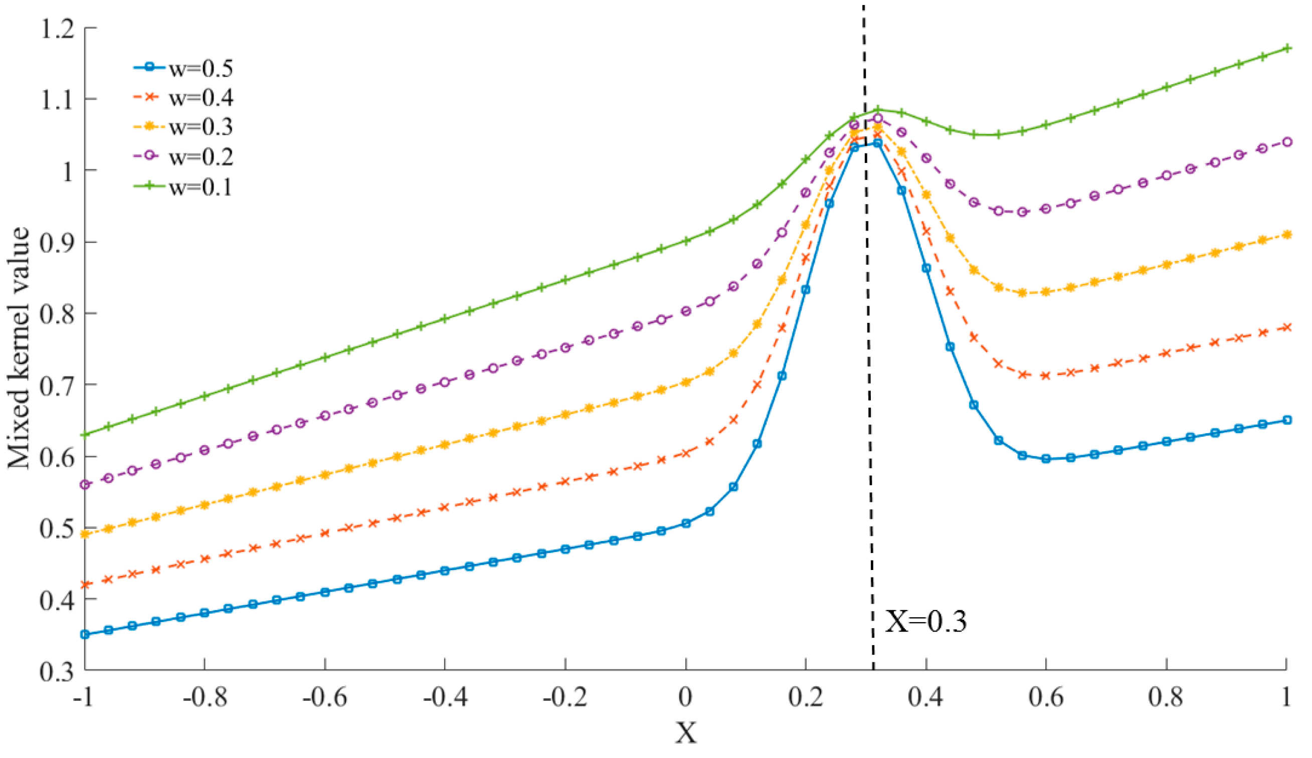
2.2. Multi-Kernel Funciton

The kernel function is the most significant component of SVR. It is used to project original low dimensional data to a higher dimensional data space, and converts a nonlinear problem into a linear problem [30]. Different kernel functions have different mapping capability, which results in different prediction accuracy. Therefore, significant efforts have been made to choose proper kernels [31,32]. Four commonly applied kernel functions are listed below:

(1)

Linear kernel function:

$$k\left(x_i,x\right)=x_i\cdot x$$

(7)

(2)

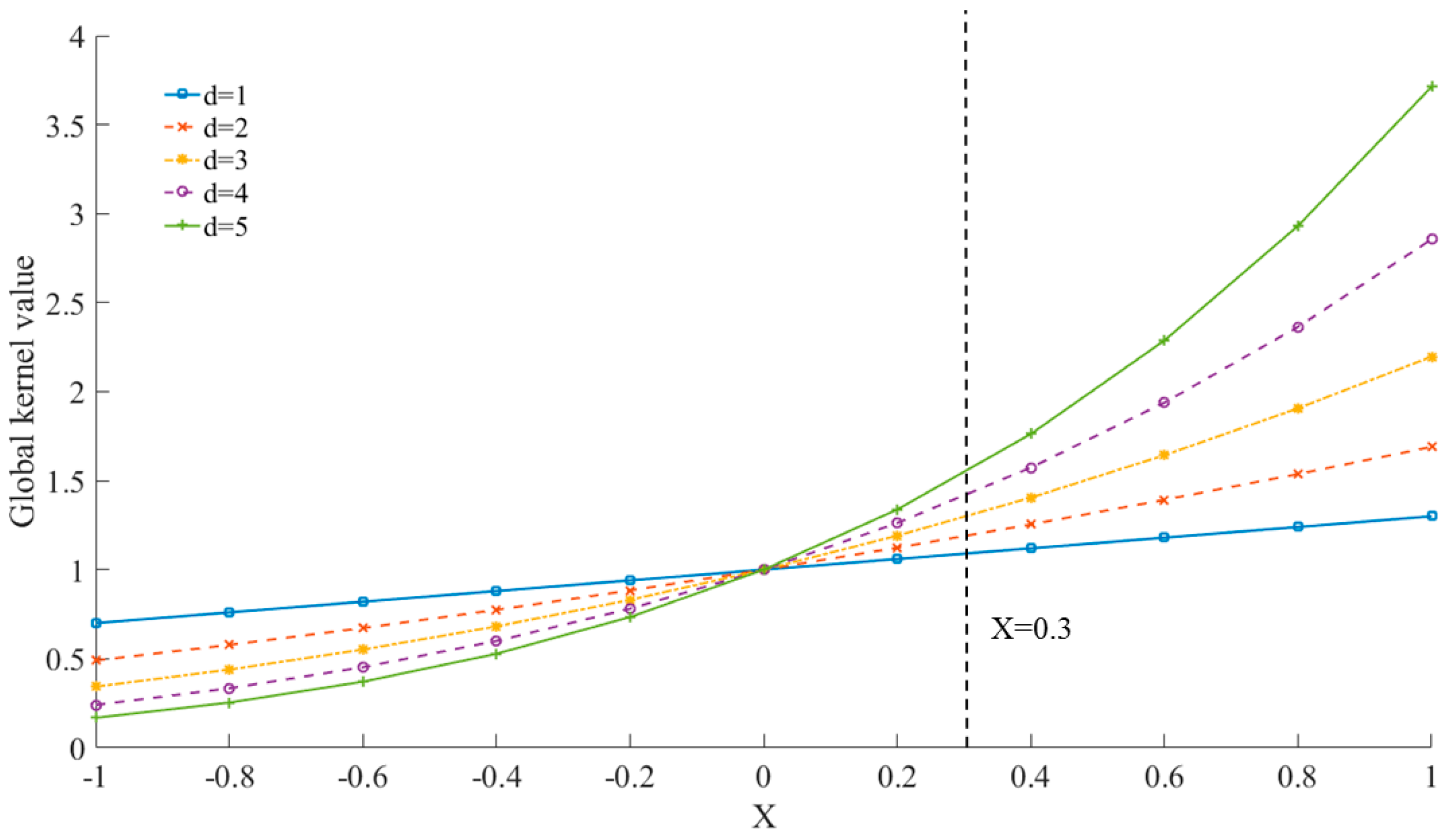
Polynomial kernel function:

$$k\left(x_i,x\right)={\left(x_i\cdot x+1\right)}^d$$

(8)

(3)

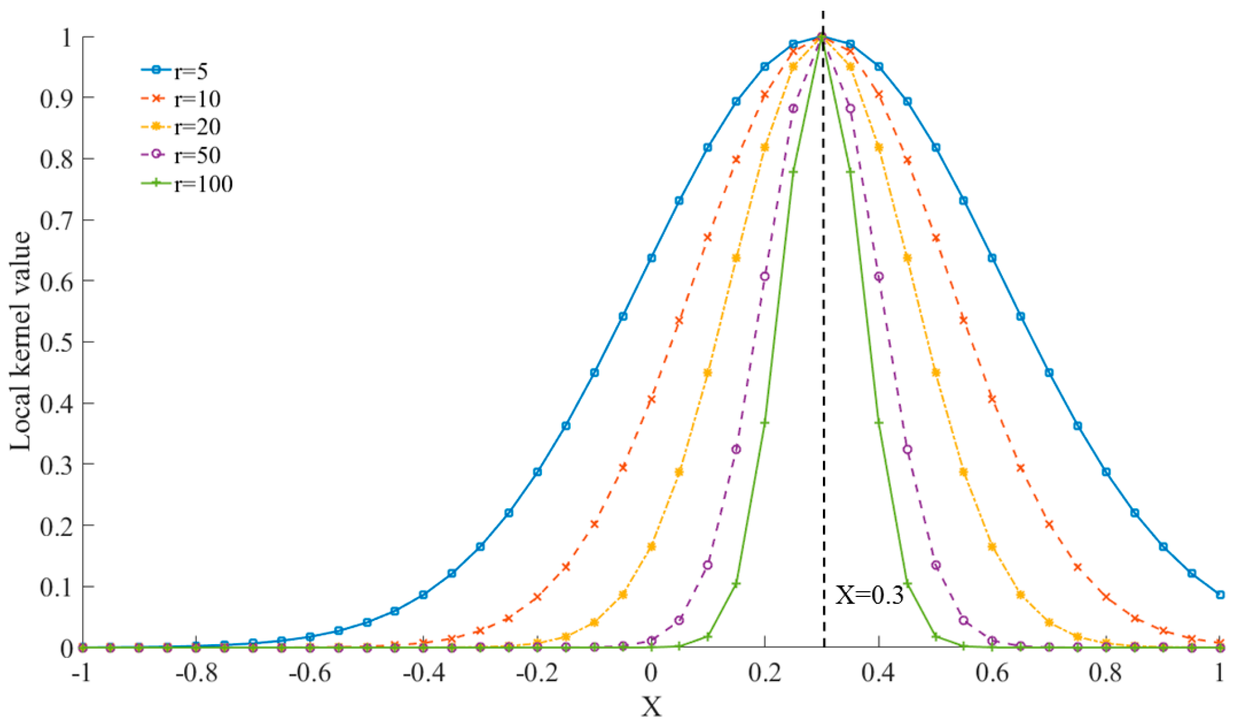
Gaussian kernel function (or RBF):

$$k(x_i,x)=\exp (-\gamma \parallel x_i-x\parallel {)}^2$$

(9)

(4)

Sigmoid kernel function:

$$k(x_i,x)=\tanh (\gamma x_i·x+\theta )$$

(10)

Generally, these kernel functions can be divided into two categories: local kernels and global kernels. There are pronounced differences in the projecting ability of different kernel functions. For the global kernel functions, such as linear kernel function and polynomial kernel function, data points far away from each other affect the kernel value and a higher order of the polynomial kernel function has better interpolation ability, while a lower order of the polynomial kernel function has better extrapolation ability. On the contrary, the local kernel functions, including Gaussian kernel function and sigmoid kernel function, allow data close to each other to have an impact on the kernel value [23,24]. The data distribution characteristics of polynomial kernel and Gaussian kernel are shown as Figure 1 and Figure 2, respectively.

Considering the advantages and disadvantage of local kernels and global kernels, we try to integrate different kernel functions to obtain one mixed-kernel function (MKF), which is shown as Equation (11). According to Mercer’s conditions, when $k_1$ and $k_2$ are allowable kernel function, then the combined kernel $k$ is also an admissible kernel.

$$k\left(x_i,x\right)=C_1{k}_1\left(x_i,x\right)+C_2{k}_2\left(x_i,x\right)\left(C_1\ge 0,C_2\ge 0\right)$$

(11)

A prevalent MKF is a mixture of the Gaussian kernel and polynomial kernel, which is defined as Equation (12):

$$k_{mix}\left(x_i,x\right)=\omega \cdot \exp {\left(-\gamma \Vert x_i-x\Vert \right)}^2+\left(1-\omega \right)\cdot {\left(x_i\cdot x+1\right)}^d\left(0\le \omega \le 1\right)$$

(12)

where $\gamma$ and $d$ are the kernel width and power exponent, respectively, and $\omega$ is the mixing coefficient. Obviously, a single kernel method can be regarded as a specific case of the MKF. That is, the MKF will be polynomial kernel when $\omega =0$, and a Gaussian kernel if $\omega =1$. Figure 3 depicts the effect of the mixing of a polynomial kernel and Gaussian kernel when test point X = 0.3, d = 1 and $\gamma$ = 50. It can be seen that the mixed kernel function possesses the merits of both the local kernel and global kernel, and able to promote fitting and generalization ability.

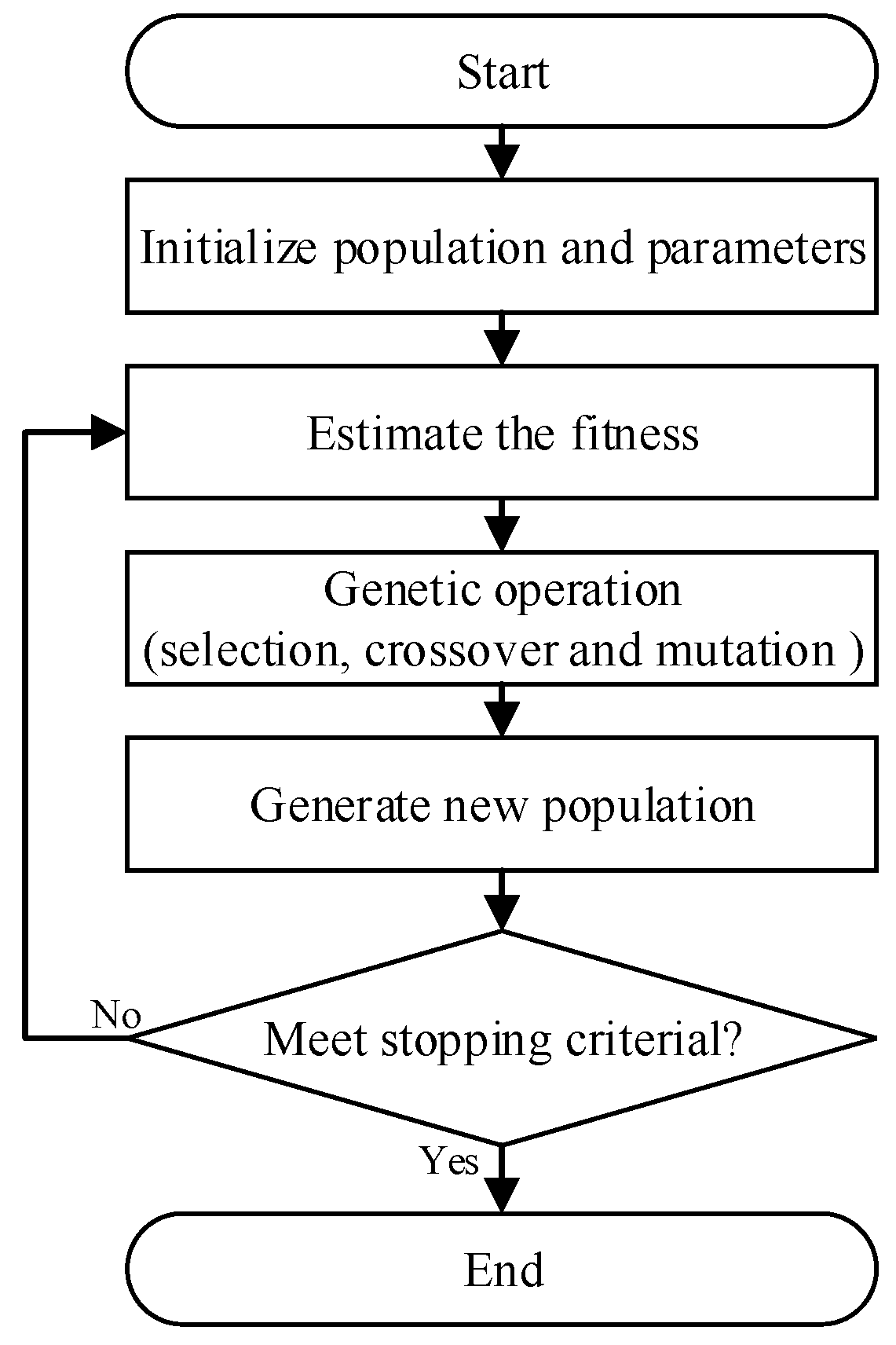
2.3. Genetic Algorithm

The genetic algorithm (GA), initially developed by John Holland in the 1970s, is a global heuristic searching and optimization technique. GA is inspired by Darwin’s principle of the “survival of the fittest” and natural evolution. GA has been applied to various optimization problems in many diverse fields and has achieved substantial progresses [33,34,35,36]. Compared with other optimization algorithms, GA is easier to converge, its calculation is more efficient and it gets a better global view of the search space because of its effective exploitation and exploration technique [37].

In general, GA starts with a randomly produced population, which represents the candidate solutions of a specific problem. Each candidate solution is called as chromosome or individual. A chromosome is composed of all concerned parameters that need to be optimized. The quality of a chromosome is assessed by a fitness function, which is established according to the objective function of the optimization problems. Genetic operations, including selection, crossover and mutation, are employed to manipulate the genetic reproduction of population during the optimization process. Selection is a process that chooses individual with higher fitness to reproduce offspring for the next generation. By this process, the population size is controlled and excellent individual is put into the next generation with a higher possibility. Crossover is a process that partial genetic information of two chosen chromosomes is exchanged by a specific way to generate new individual. Hence, individual of the next generation inherits some characteristic from each parent. The mutation operation produces new individual by randomly altering genetic information of a chromosome. The main purpose of mutation is to maintain the genetic diversity of population and avoid getting stuck in local minima. These genetic operations aforementioned will be repeated until the stopping criterion is met. A common optimization procedure of GA is shown as Figure 4.

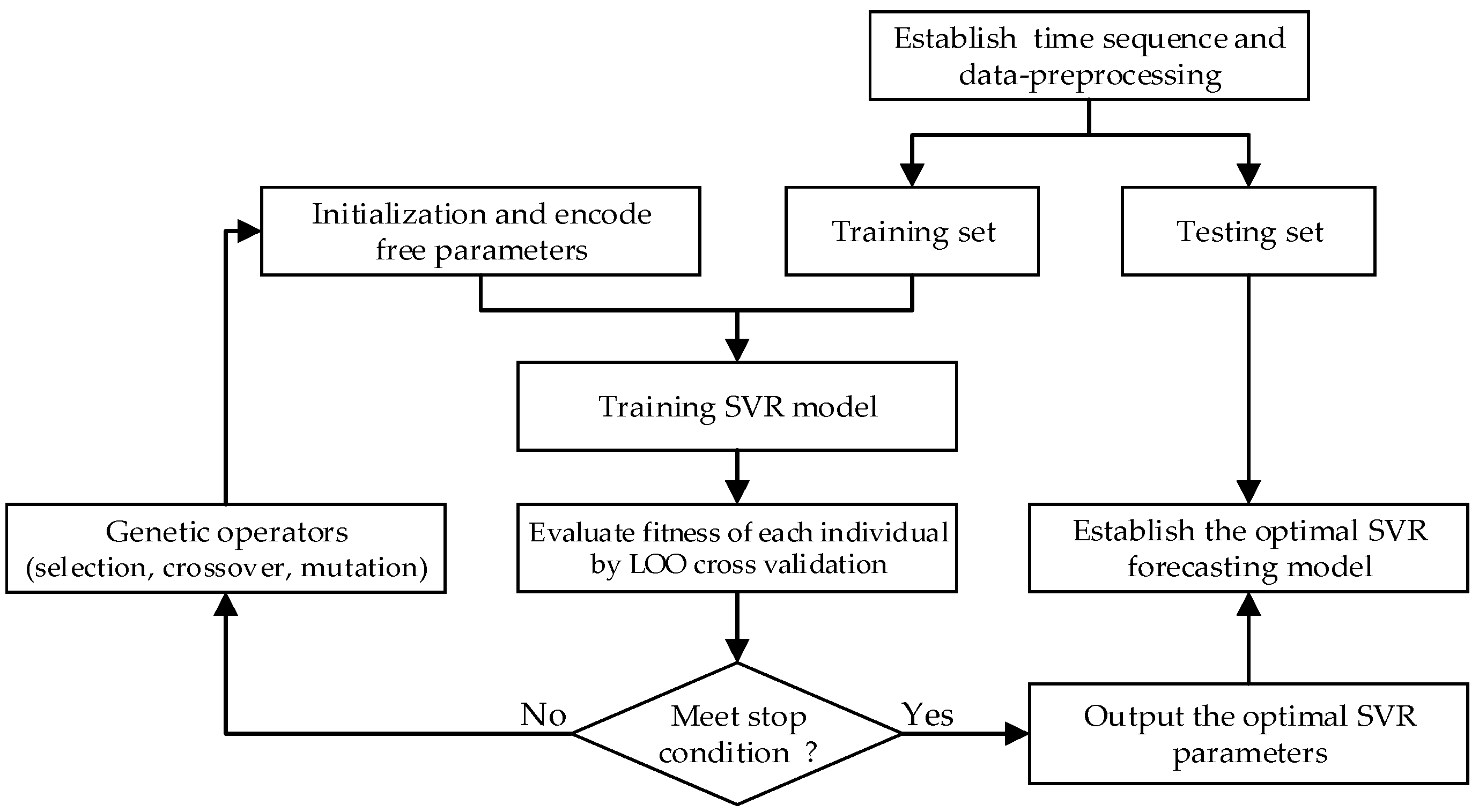
3. Procedure for Forecasting Using Proposed Regression

Usually, the concentrations of dissolved gases, including H₂, CH₄, C₂H₂, C₂H₄ and C₂H₆, are recorded or saved in chronological order. Therefore, forecasting of dissolved gas content in power transformers is treated as a non-linear time series issue. The historical dissolved gas data are used as the time sequence in the forecasting process. There are two steps to establish an effective and accurate foresting model in this study. These are, data preprocessing, training and verify the forecasting model.

3.1. Data Preprocess

For a time series problem, it is essential to preprocess the raw data due to the possibility of missing values or false data. Firstly, the input data (the historical data of H₂, CH₄, C₂H₂, C₂H₄ and C₂H₆) needs to be carefully examined in order to remove any singular values and fill in missing data by some interpolation technique. Then, normalization should be implemented prior to the construction of training and testing data to reduce estimation error and improve generalization. In this study, original data is normalized with Equation (13):

$$x_n=\frac{x_i-x_{\min }}{x_{\max }-x_{\min }}$$

(13)

where $x_i$ and $x_n$ are the data before and after normalization, respectively; $x_{\max }$ and $x_{\min }$ represent the maximum and minimum of the primary data.

Considering the case that historical data of dissolved gas may not be recorded with equal time intervals, it is necessary to convert these unequal interval series into equal time interval series to build a more convenient forecasting model. Hermite spline interpolation [19] and linear interpolation [21] are the two most popular interpolation approaches. In this paper, Hermite spline interpolation is selected to normalize primary data.

3.2. Training and Testing of The Forecasting Model

According to the historical data of dissolved gas sequence $G_n=\left\{g_1,g_2,\cdots g_n\right\}$, the training set T can be built as below:

$$T=\left\{\left(x_1,y_1\right),\left(x_2,y_2\right),\cdots \left(x_{n-m},y_{n-m}\right)\right\}\in {\left(X\times Y\right)}^{n-m}$$

(14)

where: $x_i=\left\{g_i,g_{i+1},\cdots g_{i-m+1}\right\}$ is the input vector, $y_i=\left\{g_{i+m}\right\}$ is the output value, m is the dimension of the input vector:

$$X=\left[\begin{array}{llll}{g}_1& g_2& \cdots & g_m\\ g_2& g_3& \cdots & g_{m+1}\\ ⋮& ⋮& \cdots & ⋮\\ g_{n-m}& g_{n-m+1}& \cdots & g_{n-1}\end{array}\right],Y=\left[\begin{array}{l}{g}_{m+1}\\ g_{m+2}\\ ⋮\\ g_n\end{array}\right]$$

(15)

After the historical data are divided into a training set and a testing set, a forecasting model based on MFK-SVR is trained to predict the development trend of the dissolved gas content in a power transformer. It has been mentioned in Section 2 that the free parameters of SVR and kernel functions have a great impact on the forecasting performance. Hence, GA is introduced in this paper to optimize these free parameters to improve forecasting accuracy and generalization ability. The main details of training by GA are elaborated as below:

(1) Initialization of GA and encoding parameters

In this investigation, the size of population, maximum iteration number, crossover possibility and mutation possibility are predefined at the initialization process. The chromosome, composed of free parameters (such as penalty factor C, kernel bandwidth σ, intensive loss parameter ε, power exponent d, mixing coefficient ω and so on), is set randomly. These parameters are encoded with the real code as it is suitable for complex problem and simple to use genetic operators to individuals [38]. The range and value of free parameters employed in the optimization are displayed in

Table 1. Parameters of SVR and GA.

Algorithms	Parameter	Value
SVR	Mixing coefficient ω	[0,1]
	Penalty factor C	[0.001,100]
	RBF bandwidth σ	[0.001,100]
	Epsilon ε	[0.0001,0.1]
	Polynomial degree d	[1,5]
GA	Population size	50
	Iterations	100
	Crossover probability	0.8
	Mutation probability	0.02

.

(2) Definition and calculation of fitness function

The fitness function is the core part of GA, which is used to estimate the performance of each individual. The leave one out cross-validation (LOO CV) method is adopted to calculate the forecasting accuracy. For the LOO CV method, a single sample selected from the training set is used as validation set in turn and other samples are applied as training set, then each sample is validated just once. Mean absolute percentage error (MAPE) and squared correlation coefficient (r²) are employed as fitness function to measure the quality of each chromosome and evaluate the forecasting accuracy. Generally speaking, the less MAPE, the higher forecasting accuracy. While the value of r² is limited to the range of [0,1], and the greater the value, the better forecasting performance. MAPE and r² are calculated as follows:

$$MAPE=\frac{1}{l}{\displaystyle \sum _{i=1}^l\left|\frac{f\left(x_i\right)-y_i}{y_i}\right|}$$

(16)

$$r^2=\frac{{\left(l{\displaystyle {\sum }_{i=1}^{l}f\left(x_i\right)y_i}-{\displaystyle {\sum }_{i=1}^{l}f\left(x_i\right)}{\displaystyle {\sum }_{i=1}^l{y}_i}\right)}^2}{\left(l{\displaystyle {\sum }_{i=1}^{l}f{\left(x_i\right)}^2}-{\left({\displaystyle {\sum }_{i=1}^{l}f\left(x_i\right)}\right)}^2\right)\left(l{\displaystyle {\sum }_{i=1}^l{y}_i^2}-{\left({\displaystyle {\sum }_{i=1}^l{y}_i}\right)}^2\right)}$$

(17)

where $x_i$ represents the training data; $y_i$ and $f\left(x_i\right)$ denote the actual value and forecasting value by the proposed model. l represents the size of training set.

(3) Genetic operation

Based on the estimation of the fitness value, a chromosome with higher fitness value is more likely to be selected to reproduce offspring by crossover and mutation. In this paper, roulette wheel selection, arithmetical crossover and uniform mutation are adopted to carry out genetic operations [39]. The whole process will be repeated until the maximum iteration number is reached, and then the best solution of the last generation is considered as the optimal result. The entire optimization process of the proposed approach is shown in Figure 5.

These parameters contained by the optimal solution (or chromosome) are used to establish the final forecasting model. Testing samples are set as Equation (15) described and used to calculate the forecasting valued by the established model. The index MPAE described as Equation (16), is used to test the forecasting accuracy of the proposed method. After the concerned dissolved gas contents are obtained, a local standard (GBT-7252 2001) can be employed to diagnose the working condition and incipient faults of power transformer.

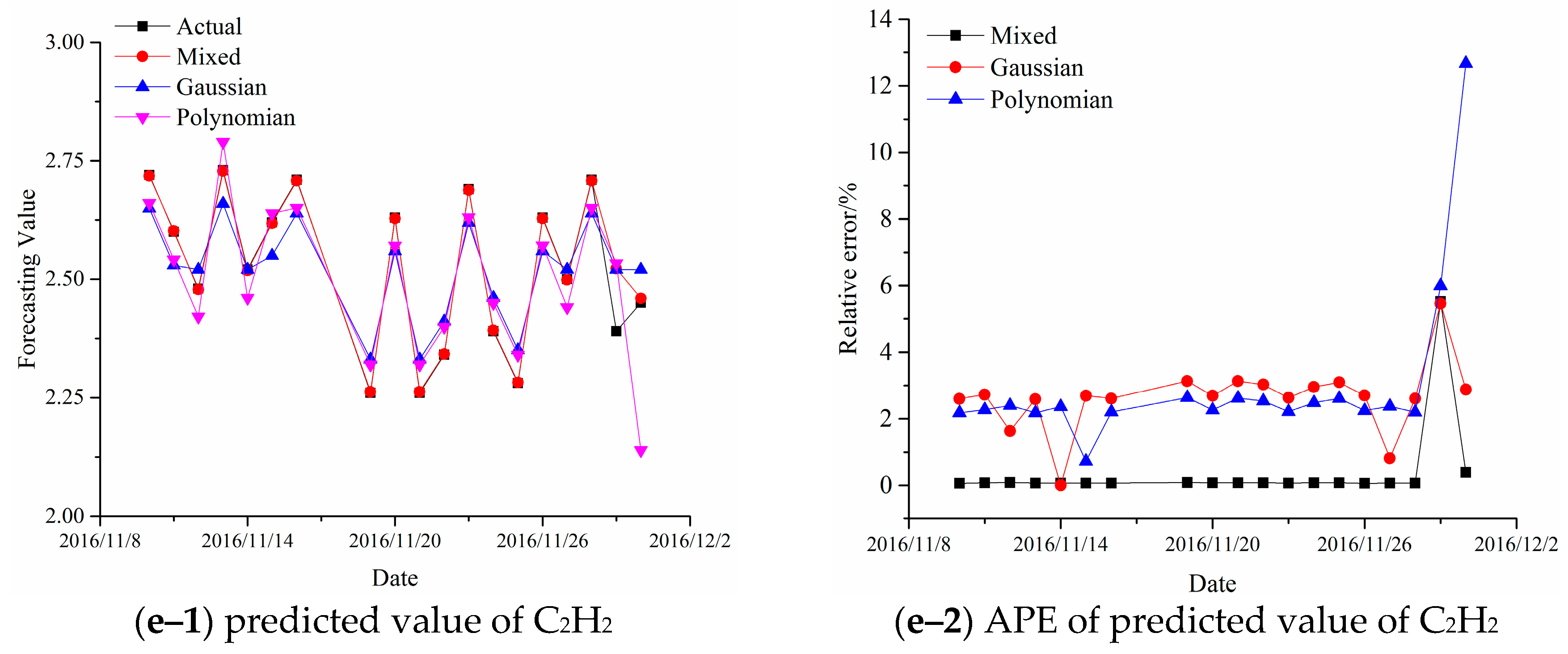
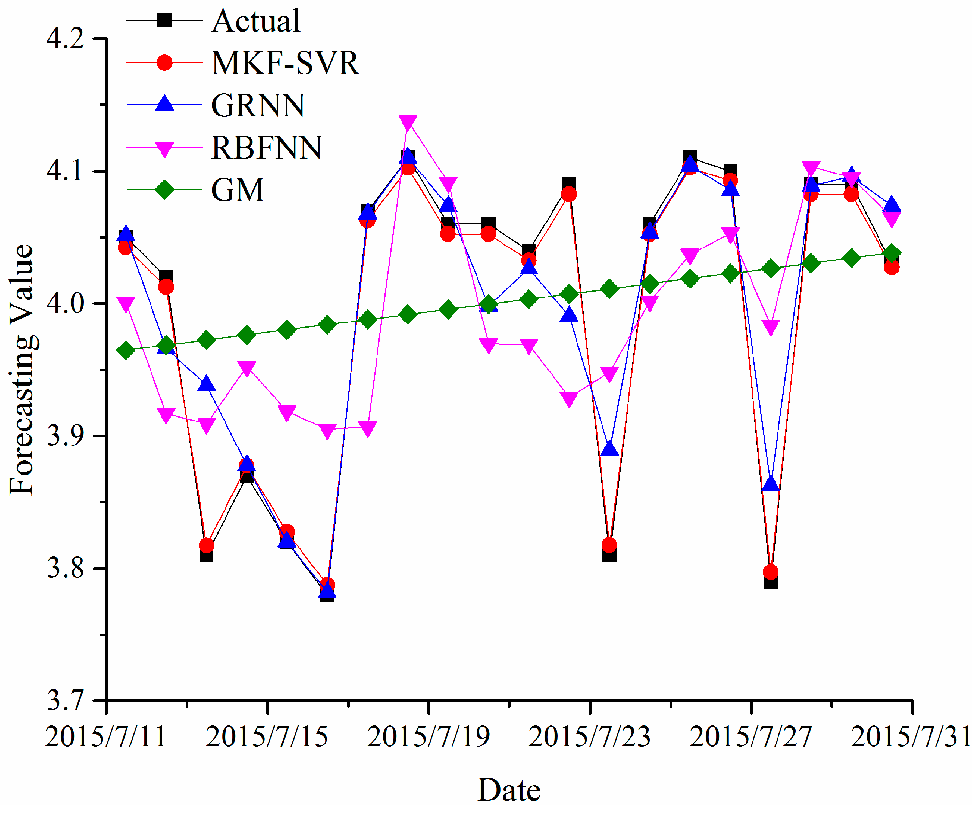
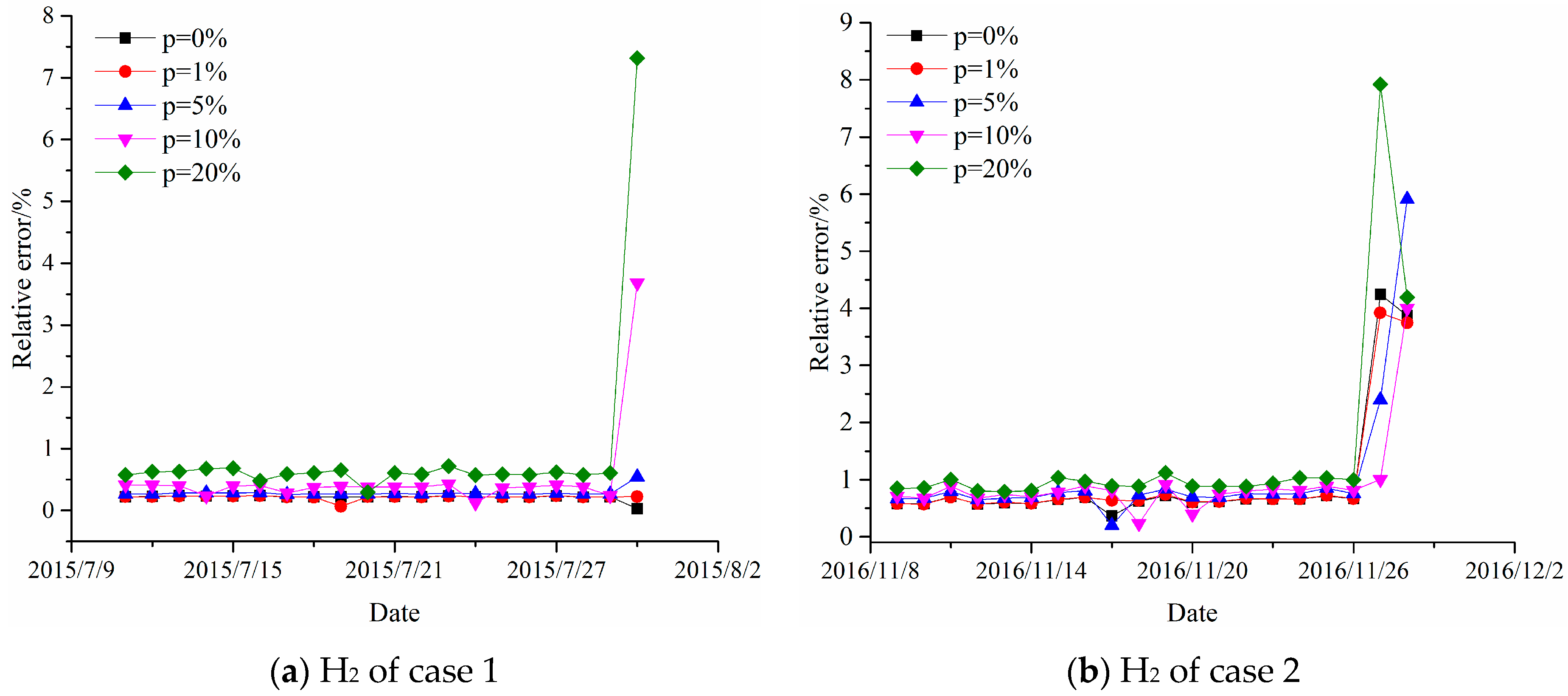
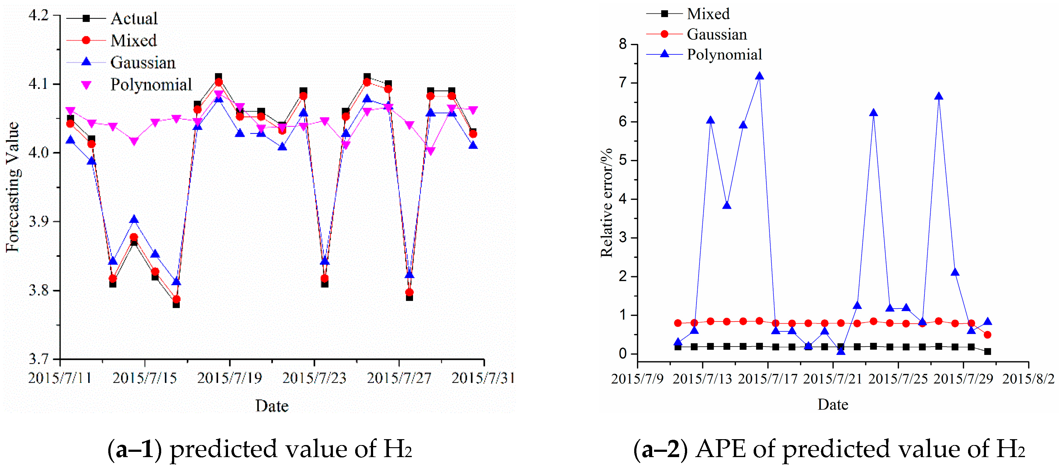
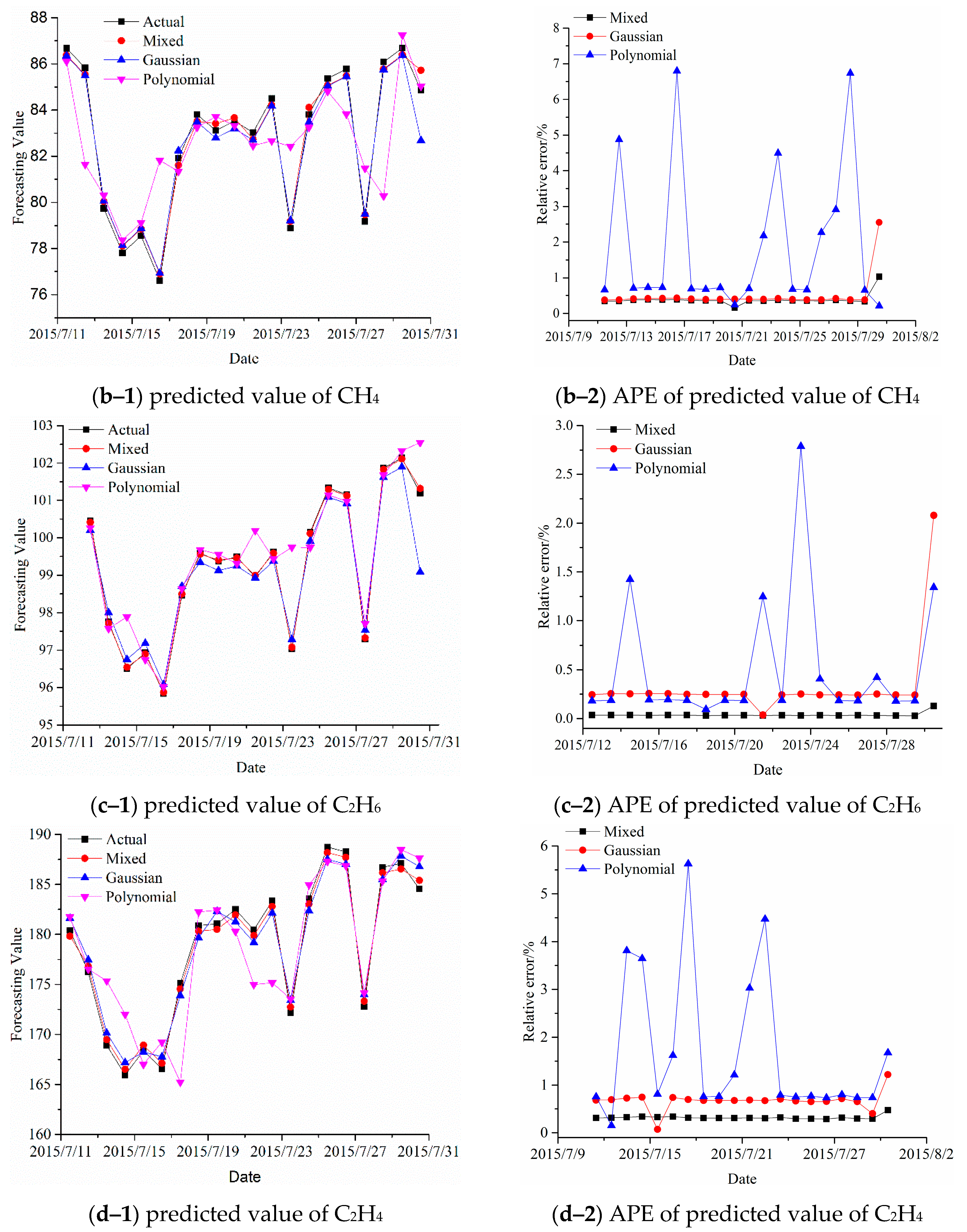
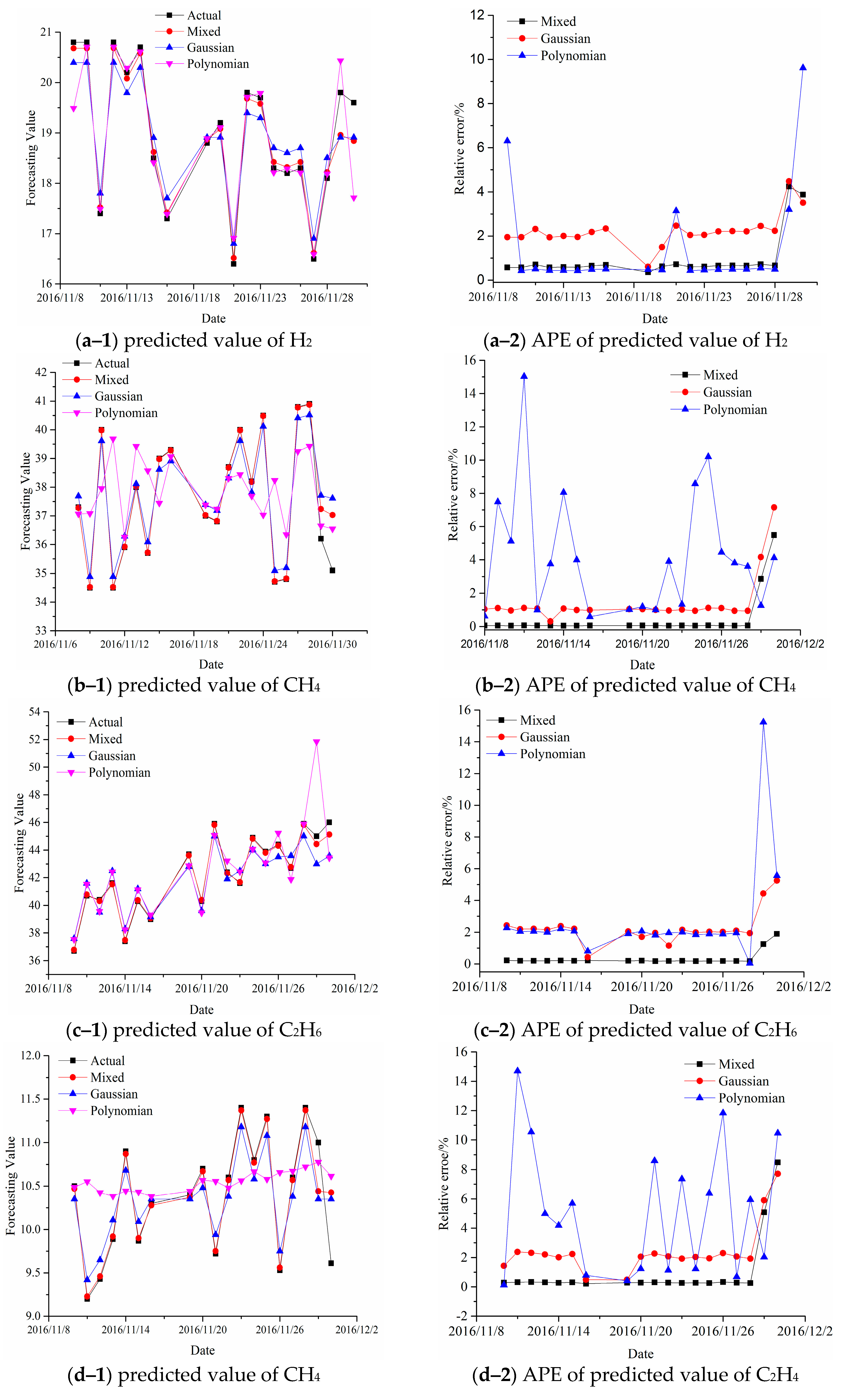
4. Experimental Results for Forecasting Dissolved Gas Content in Power Transformer Oil

Several dissolved gas content sequences of 110 kV and 220 kV power transformers from China Southern Power Grid are used to demonstrate the forecasting performance of the proposed method. These DGA data are shown in

Table 2. The dissolved gas content in a power transformer (uL/L).

Case Number	Date	H2	CH4	C2H6	C2H4	C2H2	Data Type
1	2015/7/8	3.79	80.57	97.44	167.51	0	Training
	2015/7/9	4.04	88.02	101.8	178.63	0	Training
	2015/7/10	4.04	86.55	101.4	179.98	0	Training
	2015/7/11	4.05	86.68	100.98	180.39	0	Training
	2015/7/12	4.02	85.83	100.45	176.25	0	Training
	2015/7/13	3.81	79.74	97.75	168.92	0	Training
	2015/7/14	3.87	77.81	96.51	165.95	0	Training
	2015/7/15	3.82	78.55	96.93	168.37	0	Training
	2015/7/16	3.78	76.61	95.84	166.54	0	Training
	2015/7/17	4.07	81.91	98.46	175.09	0	Training
	2015/7/18	4.11	83.81	99.59	180.88	0	Training
	2015/7/19	4.06	83.12	99.37	181.06	0	Training
	2015/7/20	4.06	83.53	99.49	182.5	0	Training
	2015/7/21	4.04	83.03	98.96	180.45	0	Training
	2015/7/22	4.09	84.51	99.62	183.36	0	Training
	2015/7/23	3.81	78.88	97.04	172.18	0	Training
	2015/7/24	4.06	83.81	100.15	183.58	0	Training
	2015/7/25	4.11	85.37	101.33	188.73	0	Training
	2015/7/26	4.1	85.78	101.16	188.25	0	Training
	2015/7/27	3.79	79.17	97.29	172.77	0	Training
	2015/7/28	4.09	86.08	101.86	186.71	0	Training
	2015/7/29	4.09	86.69	102.14	187.1	0	Training
	2015/7/30	4.03	84.85	101.19	184.53	0	Testing
2	2016/11/5	17.40	37.30	40.80	10.70	2.89	Training
	2016/11/6	17.20	40.10	38.90	10.00	2.63	Training
	2016/11/7	18.60	39.90	39.50	10.80	2.59	Training
	2016/11/8	18.20	37.30	37.20	9.84	2.97	Training
	2016/11/9	20.80	34.50	40.10	9.73	2.55	Training
	2016/11/10	20.80	40.00	36.70	10.50	2.72	Training
	2016/11/11	17.40	34.50	40.70	9.20	2.60	Training
	2016/11/12	20.80	35.90	40.40	9.43	2.48	Training
	2016/11/13	20.20	38.00	41.60	9.89	2.73	Training
	2016/11/14	20.70	35.70	37.40	10.90	2.52	Training
	2016/11/15	18.50	39.00	40.30	9.87	2.62	Training
	2016/11/16	17.30	39.30	39.00	10.30	2.71	Training
	2016/11/17	18.80	37.00	43.70	10.40	2.26	Training
	2016/11/18	19.20	36.80	40.30	10.70	2.63	Training
	2016/11/19	16.40	38.70	45.90	9.72	2.26	Training
	2016/11/20	19.80	40.00	42.40	10.60	2.34	Training
	2016/11/21	19.70	38.20	41.60	11.40	2.69	Training
	2016/11/22	18.30	40.50	44.90	10.80	2.39	Training
	2016/11/23	18.20	34.70	43.90	11.30	2.28	Training
	2016/11/24	18.30	34.80	44.40	9.53	2.63	Training
	2016/11/25	16.50	40.80	42.70	10.60	2.50	Training
	2016/11/26	18.10	40.90	45.90	11.40	2.71	Training
	2016/11/27	19.80	36.20	45.00	11.00	2.39	Testing
	2016/11/28	19.60	35.10	46.00	9.61	2.45	Testing
3	2015/7/15	8.58	7.58	6.39	1.65	0	Training
	2015/7/22	7.67	7.11	5.54	1.58	0	Training
	2015/7/29	8.25	7.33	6.59	1.85	0	Training
	2015/8/5	8.62	7	5.88	1.66	0	Training
	2015/8/12	7.92	7.64	6.56	1.62	0	Training
	2015/8/19	7.57	7.3	6.4	1.87	0	Training
	2015/8/26	8.52	7.68	5.67	1.59	0	Training
	2015/9/2	7.51	7.48	6.53	1.74	0	Training
	2015/9/9	8.14	7.67	5.64	1.6	0	Training
	2015/9/16	8.3	9.51	6.91	2.11	0	Training
	2015/9/23	7.84	9.89	7.14	2.11	0	Training
	2015/9/30	7.57	9.76	7.58	2.2	0	Training
	2015/10/7	8.68	9.52	6.95	2.11	0	Training
	2015/10/14	7.94	8.97	6.64	1.97	0	Testing
	2015/10/21	7.79	8.11	6.59	2.19	0	Testing

.

The dissolved gas data is firstly divided into training set and testing set according to data size and related references. Among them, case 1 and case 2 are sampled every day, while case 3 is sampled each week. It should be noted in this study that none singular value is eliminated and no more than 5% of data (11 out of 272) are missing in all three cases. Afterwards, normalization is implemented to improve generalization capability and reduce computational error. The whole experimental tests of the proposed approaches are conducted in the MATLAB (R2016) environment with the aid of the LIBSVM toolbox [40]. After data preprocessing and normalization, the time sequences for training set and testing set are established according to Equation (15). In this study, we test the forecasting performance of SVR models established on different single kernels, shown as Equations (7)–(10). GA is utilized to optimize the kernel parameters of ε -SVR, while LOO CV is applied to estimate the fitness to select the best choice among the candidate solutions. Numerical experiments for each model are repeated 50 times to decrease randomness within the final results. Results of the forecasting model for the training set of case 1 and case 2 are shown in

Table 3. The average forecasting performance of the training set (Case 1, 50 times).

Dissolved Gas	Kernel Type	MAPE/%			Average r2
		Max	Min	Average
H2	Linear	0.9132	0.5176	0.8227 ± 0.1018	0.0403 ± 0.0064
	Sigmoid	0.6392	0.4035	0.5484 ± 0.0801	0.0649 ± 0.0188
	Gaussian	0.6917	0.4961	0.6077 ± 0.0484	0.9958 ± 0.0018
	Polynomial	1.4718	0.8222	1.1495 ± 0.1422	0.2311 ± 0.0834
	Mixed	0.7411	0.0653	0.4144 ± 0.1764	0.9881 ± 0.0272
CH4	Linear	1.7395	0.4885	1.1726 ± 0.3569	0.1582 ± 0.0178
	Sigmoid	2.6103	0.3090	1.9075 ± 0.3687	0.0049 ± 0.0217
	Gaussian	2.7872	2.5508	2.7202 ± 0.0631	0.9838 ± 0.0067
	Polynomial	2.5717	0.2112	1.5787 ± 0.6075	0.7397 ± 0.2489
	Mixed	2.3868	0.0176	1.1702 ± 0.6838	0.9035 ± 0.1975
C2H6	Linear	2.5265	1.1519	1.4769 ± 0.3788	0.1445 ± 0.0059
	Sigmoid	3.7174	3.6412	3.6703 ± 0.0201	0.0007 ± 0.0001
	Gaussian	2.1104	2.0794	2.1027 ± 0.0006	0.9854 ± 0.0042
	Polynomial	14.6658	0.1851	7.9456 ± 6.3304	0.6667 ± 0.3152
	Mixed	1.1391	0.0105	0.4101 ± 0.2536	0.9713 ± 0.0394
C2H4	Linear	1.1385	0.0957	0.4457 ± 0.3161	0.2592 ± 0.0135
	Sigmoid	9.4499	0.2294	3.3252 ± 1.9865	0.1056 ± 0.0514
	Gaussian	2.2305	1.2168	2.0206 ± 0.2003	0.9917 ± 0.0052
	Polynomial	1.7409	0.5681	1.5511 ± 0.3239	0.6648 ± 0.1375
	Mixed	2.8552	0.4731	1.4342 ± 0.4458	0.9590 ± 0.0180

and

Table 4. The average forecasting performance of the training set (Case 2, 50 times).

Dissolved Gas	Kernel Type	MAPE/%			Average r2
		Max	Min	Average
H2	Linear	3.8211	2.2219	3.2477 ± 0.3734	0.0474 ± 0.0055
	Sigmoid	3.9352	3.8265	3.8321 ± 0.0192	0.0252 ± 0.0392
	Gaussian	4.5223	3.9864	4.1491 ± 0.1088	0.9723 ± 0.0021
	Polynomial	11.6459	6.4116	10.7708 ± 0.773	0.9598 ± 0.0197
	Mixed	4.1166	3.9798	4.0138 ± 0.0311	0.9855 ± 0.0184
CH4	Linear	5.6681	0.9128	1.9240 ± 1.6286	0.1198 ± 0.0064
	Sigmoid	35.2251	3.8304	19.7238 ± 4.9772	0.0037 ± 0.0041
	Gaussian	5.7169	5.6574	5.6986 ± 0.0139	0.9921 ± 0.0007
	Polynomial	38.4981	2.885	34.8767 ± 7.934	0.9059 ± 0.1747
	Mixed	5.4689	3.7155	4.9363 ± 0.4794	0.9877 ± 0.0309
C2H4	Linear	2.4426	0.1028	1.5430 ± 0.6544	0.5348 ± 0.0086
	Sigmoid	8.3909	0.1954	8.0604 ± 1.5451	0.0560 ± 0.0891
	Gaussian	5.5427	4.8443	5.2869 ± 0.1656	0.9694 ± 0.0239
	Polynomial	13.3713	9.7006	12.1296 ± 0.997	0.9009 ± 0.0084
	Mixed	3.18	1.5021	2.6799 ± 0.4240	0.9797 ± 0.0797
C2H6	Linear	10.2447	8.0635	9.2906 ± 0.6432	0.1107 ± 0.0112
	Sigmoid	11.3452	7.4219	10.1950 ± 1.2591	0.0051 ± 0.0074
	Gaussian	6.9159	6.7734	6.8489 ± 0.0324	0.9752 ± 0.0032
	Polynomial	20.9745	6.2449	19.6727 ± 2.644	0.8881 ± 0.0164
	Mixed	6.8225	6.8054	6.8085 ± 0.0035	0.9891 ± 0.0081
C2H2	Linear	2.5655	0.1149	1.6961 ± 0.6905	0.3469 ± 0.0059
	Sigmoid	5.2049	5.0081	5.1173 ± 0.0466	0.0006 ± 0.0005
	Gaussian	4.2828	4.1690	4.2138 ± 0.0299	0.9695 ± 0.0022
	Polynomial	10.714	4.92	9.6174 ± 1.3411	0.8397 ± 0.0134
	Mixed	3.1884	2.6363	2.9458 ± 0.1212	0.9934 ± 0.0079

, respectively.

It can be seen from Table 3 and Table 4 that, the SVR models based on linear kernel and sigmoid kernel have relatively better average MAPE than that of models established on the Gaussian kernel and polynomial kernel for all cases. However, the average r² of ε-SVR model with linear kernel or sigmoid kernel are far lower than that of models based on the other two kernels. r² provided by linear or sigmoid kernel is generally no more than 0.2 and 0.3, while the values obtained by the Gaussian and polynomial kernel are no less than 0.6 and 0.8 for case 1 and case 2, respectively.

Small r² indicates that the established model could not effectively depict the developing trends of the time series. Therefore, it is concluded that sigmoid kernel and lineal kernel are not suitable for forecasting the dissolved gas content of power transformer, and then they have not been studied further in the following investigation.

Models based on Gaussian and polynomial kernel have better squared correlation coefficient and acceptable forecasting accuracy. Therefore, we apply Gaussian and polynomial kernel to develop a novel MKF-SVR model for predicting dissolved gas contents. Forecasting results of the training set are also presented in Table 3 and Table 4, respectively. Compared with Gaussian and polynomial kernels, MKF-SVR model has slightly lower MAPE and comparative r². Among the forecasting result obtained by mixed kernel, the worst average MAPE is no more than 2% and 5%, and the lowest r² is no less than 0.95 and 0.97 for case 1 and case 2, respectively. Besides, squared correlation coefficient r² of MKF-SVR model is far better than that of models based on linear and sigmoid kernel. The results reveal that the proposed MKF-SVR model integrates the advantages of local and global kernel and manifest the superiority of the proposed approach. All cases described in Table 2 are examined with the MKF-SVR model (repeated 50 times). For the proposed model, the mixed kernel function is shown as Equation (12), and free parameters that need to be optimized have been listed in Table 1. It should be pointed out that the dimension of input vector m plays an important role in forecasting performance. An improper dimension value m will lead to undesirable forecasting results [20]. Hence, parameter m is also considered in optimization process. The optimal parameters for each gas and corresponding prediction performance are presented in

Table 5. The optimal parameters of each dissolved gas sequence.

Case No.	Dissolved Gas	Parameters						MAPE/%
		m	C	σ	ξ	d	ω	Training	Testing
1	H2	3	45.2410	66.4078	0.0228	1.8197	0.9991	0.1884	0.0645
	CH4	3	64.0668	24.8862	0.0261	1.5696	0.3923	0.3509	1.0295
	C2H6	4	72.7747	68.2022	0.0051	2.8875	0.1179	0.0332	0.1292
	C2H4	3	51.1808	77.3654	0.0538	3.7792	0.2934	0.6412	0.4713
2	H2	4	66.6143	59.5728	0.0273	1.1563	0.7490	0.6221	4.0578
	CH4	3	62.6013	53.9830	0.0033	2.0307	0.9092	0.0576	4.1765
	C2H6	5	44.8368	19.0071	0.0087	2.6108	09281	0.1917	1.5704
	C2H4	5	43.9790	68.0588	0.0134	1.0770	0.8621	0.2843	6.7836
	C2H2	5	63.0017	47.3237	0.0026	2.6083	0.7759	0.0754	2.9589
3	H2	1	2.2736	91.1686	0.0639	1.0834	0.7572	1.0224	0.8085
	CH4	1	0.1742	55.3330	0.0577	3.0111	0.0381	4.9175	3.6875
	C2H6	5	6.3558	88.1067	0.0012	2.6507	0.9225	0.0430	6.3674
	C2H4	4	70.8075	95.6627	0.0269	1.7927	0.9516	0.8165	0.0185

.

It is shown in Table 5 that the optimal value of m varies from case to case, which proves that it is necessary to tune the input vector dimension to gain a better performance. Moreover, the variation of mixing coefficient ω suggests that it is indispensable to integrate different kernels to obtain better forecasting performance. Take “H₂” of case 1 for example, according to Table 4, the minimum MAPE for Gaussian and polynomial kernel is 0.4961 and 0.8222, while for the mixed kernel, ω_G is equal to 0.9991, which means that the mapping characteristic of the kernel function is mainly determined by the Gaussian kernel. Although the weight of polynomial kernel is negligible (ω_p = 0.0009), the predicted result of the training set is greatly improved to 0.1884, which indicates that the participation of the linear kernel has greatly improved the learning ability and decreased the forecasting error. Predicted values and absolute percentage error (APE, obtained by Equation (18)) of the training set and testing set are shown in Figure 6 and Figure 7. Compared with models based on Gaussian and polynomial kernels, the MKF-SVR model can depict the variation trend of dissolved gas more accurate and more reliable. In addition, APE of models based on mixed kernels are generally lower than that of models established on other kernels. Specific forecasting values and corresponding MAPE for all training set and testing set are presented in

Table 6. The comparison of the forecasting result (testing set).

Case	Kernel Type	H2	CH4	C2H6	C2H4	C2H2
1	Actual/Mixed RBF/Polynomial	4.0300/4.0274/ 4.0101/4.0631	84.8500/85.7235/ 82.6856/85.0292	101.1900/101.3207/ 99.0858/102.5478/	184.5300/185.4030/ 186.7754/187.6218	--
	MAPE(%) (2015/7/30)	0.0645/0.4938 /0.8213	1.0295/2.5509 /0.2112	0.1292/2.0794/ /1.3418	0.4731/1.2168/ /1.6755	--
2	Actual-1/Mixed RBF/Polynomial	19.8000/18.9596/ 18.913/20.434	36.2/37.2366/ 37.707/36.548	45.0000/44.4396/ 43.0012/51.855	11.0000/10.4411/ 10.3502/7.7145	2.3900/2.5220/ 2.5206/2.5333
	Actual-2/Mixed RBF/Polynomial	19.6000/18.8412/ 18.9117/17.7143	35.1000/37.0268/ 37.6111/36.5464	46.0000/45.1275/ 43.5865/43.442	9.6100/10.4255/ 10.3503/9.017	2.4500/2.4596/ 2.5258/2.1396
	MAPE1(%) (2016/11/27)	4.2444/4.4848 /10.5353	2.8635/4.1630 /0.9613	1.2447/4.4418 /15.2333	5.0809/5.9063 /29.8636	5.5230/5.4644 /5.9832
	MAPE2(%) (2016/11/28)	3.8714/3.5102 /9.6224	5.4894/7.1538 /4.1197	1.896/5.2467 /5.5608	8.4860/7.7034 /6.1707	0.3918/3.0938 /12.6938
3	Actual-1/Mixed RBF/Polynomial	7.9400/7.9315/ 7.9160/7.5543	8.9700/9.4120/ 9.3905/9.2016	1.9700/2.0758/ 1.9234/1.4785	6.6400/6.6377/ 6.5933/5.0692	--
	Actual-2/Mixed RBF/Polynomial	7.7900/7.6724/ 7.7044/7.8758	8.1100/8.5526/ 8.8907/8.4542	2.1900/2.0287/ 1.9234/1.1178	6.5900/6.5902/ 6.5933/4.0049	--
	MAPE-1(%) (2015/10/14)	0.1068/0.3025 /4.8574	1.9171/4.6881 /2.5814	5.3716/2.3650 /24.9491	0.0340/0.7033 /23.6561	--
	MAPE-2(%) (2015/10/21)	1.5102/1.0988 /1.1014	5.4580/9.6268 /4.2437	7.3631/12.1731 /48.9590	0.0031/0.0501 /39.2284	--

. For each case, the least MAPE for forecasting value of the testing set are displayed in bold. Most of the result obtained by MKF-SVR are preferable to that of other methods. To sum up, the MKF-SVR model generally can accurately depict developing trends of dissolved gas and elevate the forecasting accuracy:

$$APE=\left|\frac{f\left(x_i\right)-y_i}{y_i}\right|$$

(18)

Furthermore, we compare the forecasting performance of MKF-SVR with other three popular methods (including GRNN, RBFNN and GM) in order to demonstrate the superiority of the proposed method. The experimental results and forecasting values of training and testing sets are presented as

Table 7. The comparison of experimental results for H₂ (Case 1).

Methods	Training Set		Testing Set
	MAPE	r2	MAPE
MKF-SVR	0.4144	0.9881	0.0645
GRNN	0.7625	0.8566	1.0893
RBFNN	2.1712	0.3478	0.8734
GM	2.6542	0.0911	0.2062

and Figure 8 (for Case 1, H₂). Table 7 shows that the proposed MKF-SVR method has the best MAPE and r² than that of other traditional methods. According to Figure 8, it can be found that, for the grey model, the forecasting value is monotonously increased, which is not accordance with the actual value at all and gives the biggest error and lowest r² due to the limitation of grey model mentioned in Section 1. In comparison with RBFNN, GRNN not only has better forecasting results, but also can depict the developing trends better. Nevertheless, these models are based on the principle of empirical risk minimization, thus the forecasting performance can be further promoted by adding extra samples. The proposed MKF-SVR method applies the principle of structural risk minimization, which make it have satisfying generalization ability with fewer samples. Moreover, it has better learning ability and prediction ability as the combination of local kernel and global kernel, which is conducive to illustrate developing trends of dissolved gas in power transformers. In conclusion, the forecasting accuracy and fitting performance of the proposed MKF-SVR model outperform that of other popular approaches.

Considering a situation that there exists bias or noisy during measurement of the dissolved gas content, which might affect the reliability and accuracy of the proposed model. Hence, the robustness of the proposed model is examined with noisy data. The noisy data is obtained by Equation (19):

$$dat{a}_{noisy}=dat{a}_{ori}(1+p*rand))\left(0\%<p\le 100\%\right)$$

(19)

where $dat{a}_{ori}$ and $dat{a}_{noisy}$ are the original data and noisy data, respectively. p denotes a percentage level of noise. rand represents a data generated by uniform distribution between 0 and 1.

When the noisy data is ready, the data preprocessing techniques mentioned in Section 3 are carried out and the proposed model with the optimal parameters is employed to forecast the dissolved gas content. Forecasting values of training set and testing set are obtained and APE is adopted to estimate the forecasting performance. Data of H₂ in case 1 and case 2 are used to demonstrate the prediction capability, and the absolute value of APE of the forecasting results at different p are shown in Figure 9.

It can be seen from Figure 9 that APE is increased as p increases, whereas, there are slight differences in the training sets for both case 1 and case 2. Although the APE value of the testing set varies greatly, for case 1, APE for the testing set is obviously increased when p is larger than 5%, while for case 2, there are minor difference in APE for the testing set when the noise level is increased from 0 to 20%. Besides, the maximum change on APE for the testing sets of both case is no more than 10%, which is acceptable in practical application. Therefore, it can be concluded from Figure 9 that the proposed model has remarkable forecasting performance and desirable robustness.

5. Conclusions

In this paper, a mixed-kernel function based support vector regression model (MKF-SVR) is proposed to forecast the dissolved gas content in power transformers. At the beginning, the forecasting performance of SVR models with single kernel function are checked and the results suggest that models based on sigmoid kernel or linear kernel are not suitable for prediction of dissolved gas content. A mixed kernel function, combined with Gaussian kernel and polynomial kernel, is applied to develop the novel MKF-SVR model. Genetic algorithm and LOO-CV are adopted to optimize free parameters. Forecasting performance of the proposed MKF-SVR model is tested by actual gas data and the results indicate that the proposed model is generally superior to single kernel function based SVR models. Moreover, prediction results of RBFNN, GRNN and GM are compared with that of MKF-SVR, and the comparison results demonstrate that the proposed model has a better forecasting accuracy and fitting capability than that of other models. Additionally, the forecasting results based on noisy data verify the desirable robustness of the proposed model. In the future, several extra factors, including oil temperature, working load and environmental condition, should be taken into consideration for forecasting the development trends of dissolved gas levels in power transformers. Besides, more kernel types and different optimization algorithms can also be investigated to improve the forecasting performance.

References

1. Kari, T.; Wen, S.; Zhao, D. An Integrated Method of ANFIS and Dempster-Shafer Theory for Fault Diagnosis of Power Transformer. IEEE Trans. Dielectr. Electr. Insul. 2018, 25, 360–371. [Google Scholar] [CrossRef]
2. Faiz, J.; Soleimani, M. Dissolved gas analysis evaluation in electrical power transformer using conventional methods: A review. IEEE Trans. Dielectr. Electr. Insul. 2017, 24, 1239–1248. [Google Scholar] [CrossRef]
3. Cheng, L.; Yu, T. Dissolved Gas Analysis Principle-Based Intelligent Approaches to Fault Diagnosis and Decision Making for Large Oil-Immersed Power Transformers: A Survey. Energies 2018, 11, 913. [Google Scholar] [CrossRef]
4. Duval, M. Dissolved Gas Analysis: It Can Save Your Transformer. IEEE Electr. Insul. Mag. 1989, 5, 22–27. [Google Scholar] [CrossRef]
5. Rogers, R. IEEE and IEC Codes to Interpret Incipient Faults in Transformers Using Gas in Oil Analysis. IEEE Trans. Electr. Insul. 1978, 13, 349–354. [Google Scholar] [CrossRef]
6. Ghoneim, S.; Taha, I.; Elkalashy, N. Integrated ANN-Based Proactive Fault Diagnostic Scheme for Power Transformer Using Dissolved Gas Analysis. IEEE Trans. Dielectr. Electr. Insul. 2016, 23, 1838–1845. [Google Scholar] [CrossRef]
7. Khatib, E.; Barco, R.; Andrades, A. Diagnosis Based on Genetic Fuzzy Algorithms for LTE Self-Healing. IEEE Trans. Veh. Technol. 2016, 65, 1639–1651. [Google Scholar] [CrossRef]
8. Mansour, D. Development of a New Graphical Technique for Dissolved Gas Analysis in Power Transformers Based on the Five Combustible Gases. IEEE Trans. Dielectr. Electr. Insul. 2015, 22, 2507–2512. [Google Scholar] [CrossRef]
9. Piotr, M.; Yann, L. Statistical machine learning and dissolve gas analysis: A Review. IEEE Trans. Power Deliv. 2012, 27, 1791–1799. [Google Scholar]
10. Wang, M. Grey-Extension Method for Incipient Fault Forecasting of Oil-Immersed Power Transformer. Electr. Power Compon. Syst. 2010, 32, 959–975. [Google Scholar] [CrossRef]
11. Pereira, F.; Bezerra, F.; Junior, S. Nonlinear Autoregressive Neural Network Models for Prediction of Transformer Oil-Dissolved Gas Concentrations. Energies 2018, 11, 1694. [Google Scholar] [CrossRef]
12. Lin, J.; Sheng, G.; Yan, Y. Prediction of Dissolved Gas Concentrations in Transformer Oil Based on the KPCA-FFOA-GRNN Model. Energies 2018, 11, 225. [Google Scholar] [CrossRef]
13. Shaban, K.B.; EI-Hag, A.H.; Benhmed, K. Prediction of Transformer Furan Levels. IEEE Trans. Power Deliv. 2016, 31, 1778–1779. [Google Scholar] [CrossRef]
14. Weron, R. Electricity price forecasting: A review of the state-of-the-art with a look into the future. Int. J. Forecast. 2014, 30, 1030–1081. [Google Scholar] [CrossRef]
15. Cinotti, S.; Gallo, G.; Ponta, L. Modeling and forecasting of electricity spot-prices: computational intelligence VS classical econometrics. AI Commun. 2014, 27, 301–314. [Google Scholar]
16. Liao, R.; Zheng, H.; Grzybowski, S. Particle swarm optimization-least square support vector regression based forecasting model on dissolved gas in oil-filled power transformer. Electr. Power Syst. Res. 2011, 81, 2074–2080. [Google Scholar] [CrossRef]
17. Liao, R.; Bian, J.; Yang, L. Forecasting dissolved gas content in power transformer oil based on weakening buffer operator and least square support vector machine–Markov. IET Gener. Transm. Dis. 2011, 6, 142–151. [Google Scholar] [CrossRef]
18. Zheng, H.; Zhang, Y.; Liu, J. A novel model based on wavelet LS-SVM integrated improved POS algorithm for forecasting of dissolved gas contents in power transformer. Electr. Power Syst. Res. 2018, 155, 196–205. [Google Scholar] [CrossRef]
19. Zhang, Y.; Wei, H.; Yang, Y. Forecasting of Dissolved gas in Oil-immersed Transformers Based upon Wavelet LS-SVM Regression and PSO with Mutation. Energy Procedia 2016, 104, 38–43. [Google Scholar] [CrossRef]
20. Fei, S.; Liu, C.; Miao, Y. Support vector machine with genetic algorithm for forecasting of key-gas ratios in oil-immersed transformer. Expert Syst. Appl. 2009, 36, 6326–6331. [Google Scholar] [CrossRef]
21. Fei, S.; Sun, Y. Forecasting dissolved gas content in power transformer oil based on support vector machine with genetic algorithm. Electr. Power Syst. Res. 2008, 78, 507–514. [Google Scholar] [CrossRef]
22. Fei, S.; Wang, M.; Miao, Y. Particle swarm optimization-based support vector machine for forecasting dissolved gas content in power transformer oil. Energy Convers. Manag. 2009, 50, 1604–1609. [Google Scholar] [CrossRef]
23. Cheng, K.; Lu, Z.; Wei, Y. Mixed kernel function support vector regression for global sensitivity analysis. Mech. Syst. Signal. Appl. 2017, 96, 201–214. [Google Scholar] [CrossRef]
24. Zhu, X.; Huang, Z.; Shen, H. Dimensionality reduction by Mixed Kernel Canonical Correlation Analysis. Pattern Recognit. 2012, 45, 3003–3016. [Google Scholar] [CrossRef]
25. Li, S.; Fang, H.; Liu, X. Parameter optimization of support vector regression based on sine cosine algorithm. Expert Syst. Appl. 2018, 91, 63–71. [Google Scholar] [CrossRef]
26. Wu, L.; Cao, G. Seasonal SVR with FOA algorithm for single-step and multi-step ahead forecasting in monthly inbound tourist flow. Knowl.-Based Syst. 2016, 110, 157–166. [Google Scholar]
27. Li, W.; Xuan, Y.; Li, H. Hybrid Forecasting Approach Based on GRNN Neural Network and SVR Machine for Electricity Demand Forecasting. Energies 2017, 10, 44. [Google Scholar] [CrossRef]
28. Peng, L.; Fan, G.; Huang, M. Hybridizing DEMD and Quantum PSO with SVR in Electric Load Forecasting. Energies 2016, 9, 221. [Google Scholar] [CrossRef]
29. Huang, M. Hybridization of Chaotic Quantum Particle Swarm Optimization with SVR in Electric Demand Forecasting. Energies 2016, 9, 426. [Google Scholar] [CrossRef]
30. Zhong, Z.; Carr, T. Application of mixed kernels function (MKF) based support vector regression model (SVR) for CO2—Reservoir oil minimum miscibility pressure prediction. Fuel 2016, 184, 590–603. [Google Scholar] [CrossRef]
31. Wu, D.; Wang, Z.; Chen, Y. Mixed-kernel based weighted extreme learning machine for inertial sensor based human activity recognition with imbalanced dataset. Neurocompuing 2016, 190, 35–49. [Google Scholar] [CrossRef]
32. Zhang, Y.; Wang, Y.; Zhou, G. Multi-kernel extreme learning machine for EEG classification in brain-computer interfaces. Expert Syst. Appl. 2018, 96, 302–310. [Google Scholar] [CrossRef]
33. Liu, Y.; Wang, R. Study on network traffic forecast model of SVR optimized by GAFSA. Chaos Solitons Fractals 2016, 89, 153–159. [Google Scholar] [CrossRef]
34. Wang, S.; Hae, H.; Kim, J. Development of Easily Accessible Electricity Consumption Model Using Open Data and GA-SVR. Energies 2018, 11, 373. [Google Scholar] [CrossRef]
35. Gholamalizadeh, E.; Kim, M. Multi-Objective Optimization of a Solar Chimney Power Plant with Inclined Collector Roof Using Genetic Algorithm. Energies 2016, 9, 971. [Google Scholar] [CrossRef]
36. Li, C.; Zhai, R.; Yang, Y. Optimization of a Heliostat Field Layout on Annual Basis Using a Hybrid Algorithm Combining Particle Swarm Optimization Algorithm and Genetic Algorithm. Energies 2017, 10, 1924. [Google Scholar] [Green Version]
37. Wang, B.; Yang, Z.; Lin, F. An Improved Genetic Algorithm for Optimal Stationary Energy Storage System Locating and Sizing. Energies 2014, 7, 6434–6458. [Google Scholar] [CrossRef] [Green Version]
38. Haghrah, A.; Mohammadi, B.; Seyedmonir, S. Real coded genetic algorithm approach with random transfer vectors-based mutation for short-term hydrothermal scheduling. IET Gener. Transm. Distrib. 2013, 9, 75–89. [Google Scholar] [CrossRef]
39. Herrera, F.; Lozano, M.; Verdegay, J. Tackling Real-Coded Genetic Algorithms: Operators and Tools for Behavioural Analysis. Artif. Intell. Rev. 1998, 12, 265–319. [Google Scholar] [CrossRef]
40. Chang, C.; Lin, C. A library for support vector machines. ACM T. Intell. Syst. Technol. 2011, 2, 27:1–27:27. [Google Scholar]
Figure 1. Data distribution of global kernel (polynomial kernel, test point X = 0.3).
Energies 11 02437 g001
Figure 2. Data distribution of local kernel (Gaussian kernel, test point X = 0.3).
Energies 11 02437 g002
Figure 3. Data distribution of a mixed kernel (Gaussian kernel & polynomial kernel, test point X = 0.3).
Energies 11 02437 g003
Figure 4. Flowchart of the optimization procedure of GA.
Energies 11 02437 g004
Figure 5. Flowchart of parameter optimization of MKF-SVR.
Energies 11 02437 g005
Figure 6. Forecasting value and APE of SVR model with different kernels (Case 1).
Energies 11 02437 g006aEnergies 11 02437 g006b
Figure 7. Forecasting value and APE of SVR model with different kernels (Case 2).
Energies 11 02437 g007aEnergies 11 02437 g007b
Figure 8. The forecasting values of H2 (Case 1).
Energies 11 02437 g008
Figure 9. APE of forecasting result with different p.
Energies 11 02437 g009