Optimum Thermal Concentration of Solar Thermoelectric Generators (STEG) in Realistic Meteorological Condition

Abstract

Global warming and air pollution concerns make renewable energies inevitable. Thermoelectric (TE) generators—solid-state devices which can convert thermal energy into electricity—are one of the candidates to capture the energy of the sun’s rays. Impact of high thermal on flat panel Solar Thermoelectric Generator (STEG) performance is known. In this research, a method to optimize thermal concentration in realistic terrestrial condition is introduced. To this end, a Simulink model of the STEG was developed, and module performance curves are determined. According to the results, Thermal concentration in realistic condition is more than double, compared to standard condition. The efficiency of the STEG was 4.5%, 6.8%, and 7.7% when the module figure of merit (ZT) was set to 0.8, 1.2, and 1.5, respectively, in locations with a higher ratio of diffused radiation (e.g., Aalborg and Denmark). These values corresponded to 70%, 106%, and 121% of the electrical power produced by parabolic troughs under the same meteorological condition. Furthermore, the possibility of controlling the ratio of heat and electricity in the cogeneration system is possible by controlling the heating flow or electric current. Heating flow can be controlled by the electrical current in STEG over 17 percent of its value in optimum condition.

1. Introduction

The thermoelectric effect has been known since 1821 when Thomas Seebeck observed the electric potential by applying a temperature gradient. However, low efficiency restricted their applications to thermocouple sensors and niche places, such as space exploration [1]. The first Solar Thermoelectric Generator (STEG) with the efficiency of 0.63% was introduced by Telkes in 1954 [2], who predicted that solar absorbers could increase efficiency to 1.05%. Promising theoretical [3] and experimental [4] studies in the 1990s revealed thermoelectric (TE) properties could significantly enhanced, paving the way for further studies. On the other hand, green energy has become increasingly important during the past few decades, mostly due to global warming and air pollution concerns [5,6,7]. There are three major types of solar plants, including photovoltaic, flat, and concentrated thermal absorbers. Photovoltaic can directly convert photons energy to electricity, where based on semiconductor band gap theory efficiency is limited to 32.8% for single-junction GaAs cell. However, practical obstacles make the real efficiency a fraction of the theoretical one [8]. Solar thermal collectors absorb the energy of the sun’s rays, which is typically used to provide warm water [9]. Having a large emissivity in the solar wavelengths and a small emissivity in the long wavelengths, selective solar absorbers can convert more than 95% of solar energy into heat [10], which leads to efficiency within the range of 40 to 60% with working fluid temperature below 100 $℃$ [11]. Parabolic troughs were present in 96.3% of installed concentrated solar power plants (CSPs) until 2011, with the peak efficiency of 21%. Meanwhile, the electricity efficiency for achieved system level of sun rays is in the range of 10 to 15% with 18% mid-term perspective [12,13]. A major drawback is that CSPs only capture DNI rays and their performance is degraded under cloudy conditions [13].

TEGs require a high temperature difference to show good performance [2,14] while the solar flux is constant. Different types of STEGs, hybrid photovoltaic–thermoelectric generators, and cogeneration of heat and electricity by concentrated photovoltaic systems were reviewed in previous studies [15,16,17,18,19,20,21,22,23,24,25,26,27,28]. Moreover, concentrated optical systems [15,16] and flat-panel STEGs, which use the thermal concentration (TC) [2] to conduct heat in the absorber laterally to concentrate heat where the TEG is located, have been evaluated before.

In 2017, Olsen et al. [15] designed a high-temperature STEG with segmented n-type leg consisting of skutterudite and $L{a}_{3}T{e}_4$, and p-type leg including skutterudite and $Y{b}_{14}Mn21S{b}_{11}$ in the designed thermal/optical cavity, so that the whole complement of light wavelengths could be captured and an efficiency of 15% could be achieved. In the aforementioned research, the efficiency of 18% was predicted by higher optical concentration (200–300 Suns and $T_h=1000 ℃$) and active cooling on the cold side of the TEG. This shows a 2-fold gain, compared to experimental results [16] in 2016 with efficiency of 7.4% (TC = 211, selective absorber, vacuum insulators, segmented legs, and $T_h=600 ℃$).

Among several researchers who applied TC concepts [17,18,19,20,21], Kraemer et al. [19] carried out an interesting study, reporting the highest STEG efficiency of 5% without any optical concentrator. They designed a flat-panel STEG with a selective absorber and nanostructured thermoelectric materials. According to the aforementioned research, efficiency was in the range of 4.3 to 5.2% at AM1.5 while the ZT material was equal to 1.04 at an optimum temperature of $100 ℃$ [15,22]. Kraemer et al. also predicted an efficiency of 14% by a more efficient material with ZT = 2 and an optical concentration of 10. Clearly, the concentrated STEGs show better performance compared to flat panels. Nonetheless, STEGs have some disadvantages, including the complexity of the system and the fact they can only capture DNI [16]. Generally, concentrating systems are only economical for locations with DNI above $1800 {\mathrm{kWkm}}^{-2}{\mathrm{year}}^{-1}$ [13], this restricts the application of concentrator systems in low-DNI locations.

The theoretical studies [23] on flat-panel STEGs include several simplifications, such as temperature independent material properties, geometry-independent radiation heat losses, and neglecting thermal/electrical contact resistances. A more detailed model for STEGs was proposed by Kraemer et al. [24], who considered all of the aforementioned effects and compared the model with previous studies in order to highlight the importance of each assumption. Furthermore, some modified simplifications were introduced to maintain the accuracy of the model and reduce the computational time. By considering a geometric ratio ($L/A_{TEG}$) to determine thermal resistance of the STEG for cold side temperatures between 25 and 100 °C, the optimum geometric ratio was determined to be between 0.32 and 0.41 m. These researchers also calculated the output energy for the period of one day, concluding that the results were not exactly sensitive to the geometric ratio. However, their model was unable to generalize this conclusion throughout the year due to the variation of the temperature and radiation.

Figure 1 shows solar irradiation of two locations with different solar incident specifications, including Aalborg in the North of Denmark with high diffused irradiance and low global irradiance and Gibraltar city in Gibraltar with lower diffused irradiance and higher global irradiance. In contrast to Gibraltar, annual direct irradiance in Aalborg is below the minimum DNI required for concentrated systems ($1800{\mathrm{kWkm}}^{-2}{\mathrm{year}}^{-1})$. With respect to the actual terrestrial conditions (e.g., air temperature and irradiance in a period of one year), and high dependency of STEG performance on thermal concentration value and cold side temperature, the optimization objective of the STEG must be achieved to maximize the efficiency for a year instead of a specific standard test condition (STC) in order to avoid obtaining yearly performance below the expected rate.

Based on the above argument, this work aims to develop a method to optimize the thermal concentration of STEG with respect to realistic terrestrial conditions. To end this goal, a 1D model of STEG was developed in MATLAB Simulink where TEG performance was computed over a wide range of solar radiation and cold side temperature. The model simulates STEG behavior, and it can control current, voltage, and cold side temperature. To optimize TC over a year, the optimum values of each day are averaged. This is carried out in a loop to check the peak hot side temperature and adjust TC to protect module.

2. Materials and Methods

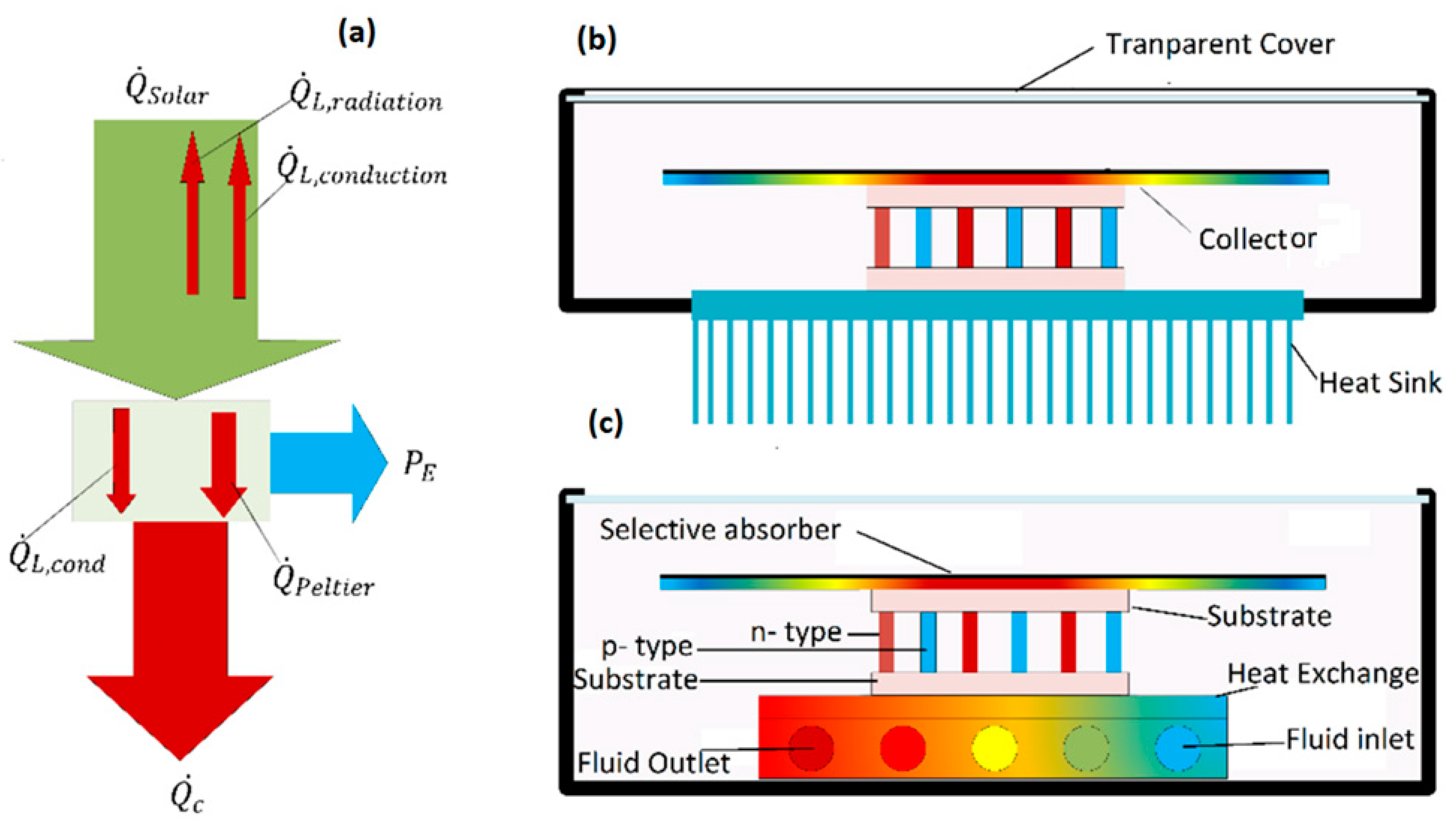
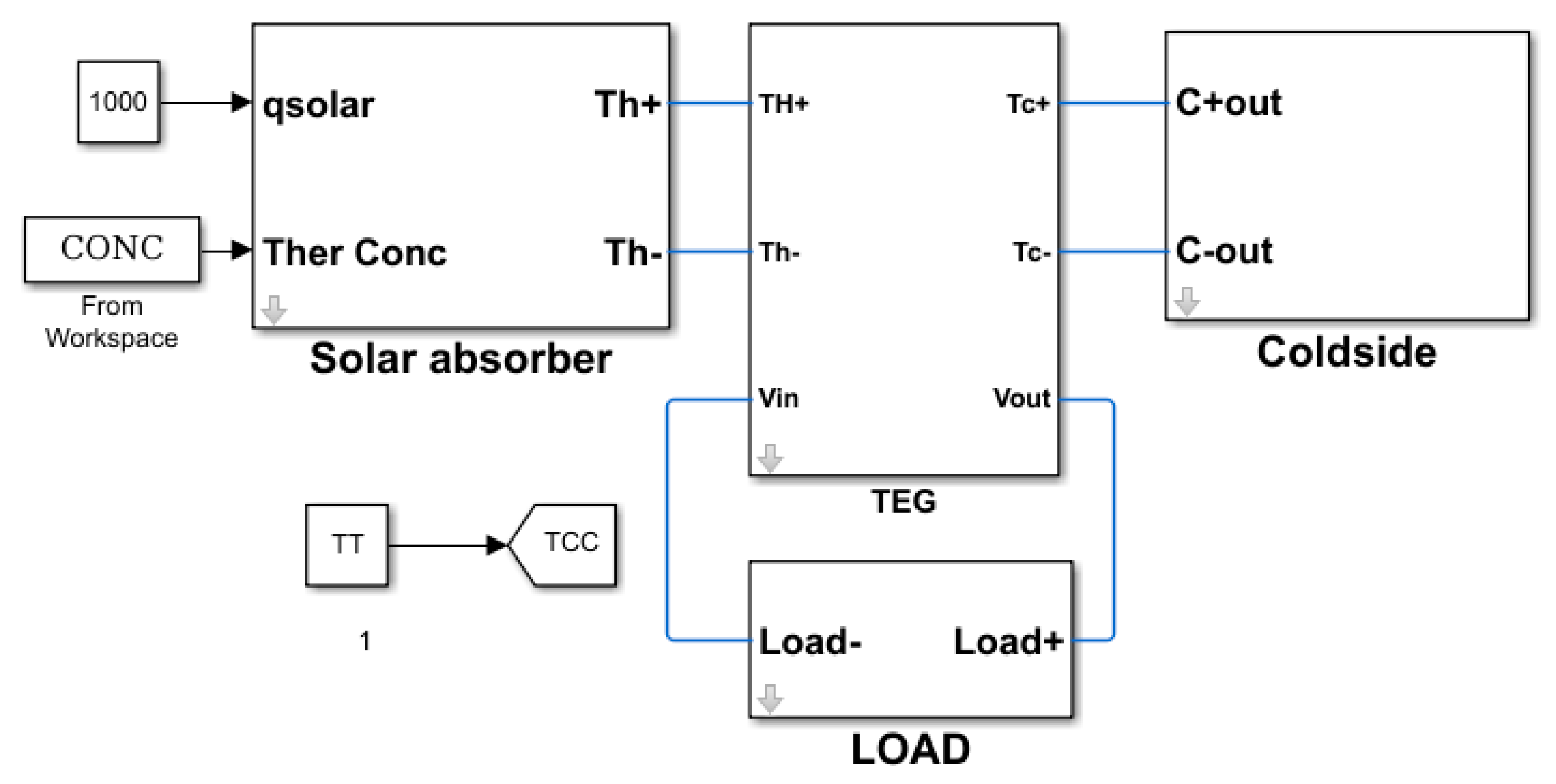
2.1. Solar TEG Model

Electrical equivalent model for thermal studies, which is based on the analogy between thermal and electrical parameters (

Table 1. Analogy between thermal and electrical parameters in this study.

Thermal Quantity	Electrical Equivalent
Temperature, $\left[\mathrm{K}\right]$	Voltage, [V]
Heat flow, $\dot{Q}=\left(\frac{\mathsf{\Delta }T}{R_{th}}\right)\left[\mathrm{W}\right]$	Current, $I=\left(\frac{\mathsf{\Delta }V}{R}\right)\left[\mathrm{A}\right]$
Thermal conductivity, $\kappa \left[\frac{\mathrm{W}}{\mathrm{mK}}\right]$	Electrical conductivity, $\sigma \left[\frac{1}{\mathsf{\Omega }\mathrm{m}}\right]$
Thermal mass, $C_{th}\left[\frac{\mathrm{J}}{\mathrm{K}}\right]$	Electrical capacitance, [F]
ermal resistance, $R_{th}\left[\frac{\mathrm{K}}{\mathrm{W}}\right]$	Electrical resistance, $R\left[\mathsf{\Omega }\right]$

), was used to simulate thermoelectric generators [26,27,28,29]. In the present study, MATLAB Simulink Simscape library was exploited to develop the model. The model includes the solar absorber, TEG, cold side heat exchanger, and electrical load. In Figure 2, the schematic of the two conceptual designs of the STEGs, which use a selective absorber, as well as vacuum insulated chamber and transparent glass are presented.

The energy flow is shown in Figure 2a. The sun irradiance $({\dot{Q}}_{Solar})$ is absorbed by the selective absorber, passes through the collector plate, and then flows through the thermoelectric legs (Figure 2b). The thermal concentration, the ratio between the collector $\left(A_{Coll}\right)$, and TEG $\left(A_{TEG}\right)$ surface areas are above 100, which causes high temperature and radiative losses $({\dot{Q}}_{L, Rad})$. Vacuum insolation can minimize conductive losses $({\dot{Q}}_{L, Cond})$. Moreover, the thermal conductivity in a typical vacuumed solar collector is in the order of ${10}^{-3}\mathrm{W}/\mathrm{mK}$. In Figure 2b, the dissipated heat $({\dot{Q}}_C)$ rejects to ambient. Meanwhile, the rejected heat is an input of the heat for the CHP system, presented in Figure 2c. Energy balance equations of the system are, as follows:

$${\dot{Q}}_{Solar}={\dot{Q}}_{L,Rad}+{\dot{Q}}_{L,Cond}+P_E+{\dot{Q}}_C$$

(1)

$${\dot{Q}}_C={\dot{Q}}_{Peltier}+{\dot{Q}}_{Cond}$$

(2)

In STEGs, efficiency of the system is the product of thermal efficiency and electrical efficiency where:

$${\eta }_{R\to H}=\frac{{\dot{Q}}_{Solar}-{\dot{Q}}_{L,Rad}-{\dot{Q}}_{L,Cond}}{{\dot{Q}}_{Solar}}$$

(3)

$${\eta }_{H\to E}=\frac{P_E}{{\dot{Q}}_{Solar}-{\dot{Q}}_{L,Rad}-{\dot{Q}}_{L,Cond}}=\frac{P_E}{P_E+{\dot{Q}}_C}$$

(4)

$$\eta =({\eta }_{R\to H})\times ({\eta }_{H\to E})$$

(5)

Thermal efficiency (3) depends on absorber properties, insulation quality, and temperature difference, while electrical efficiency Equation (4) is the function of TEG properties and the temperature difference across the TEG. The temperature must be optimized due to the inverse effect of the temperature difference on the thermal and electrical efficiencies. A STEG system includes a solar absorber, a TEG device, cold side, and an electrical load, as shown in Figure 3. Each part of the system is masked to sweep across variables by assigning the thermal concentration and cold side temperature from the MATLAB workspace.

2.2. Solar Absorber Model

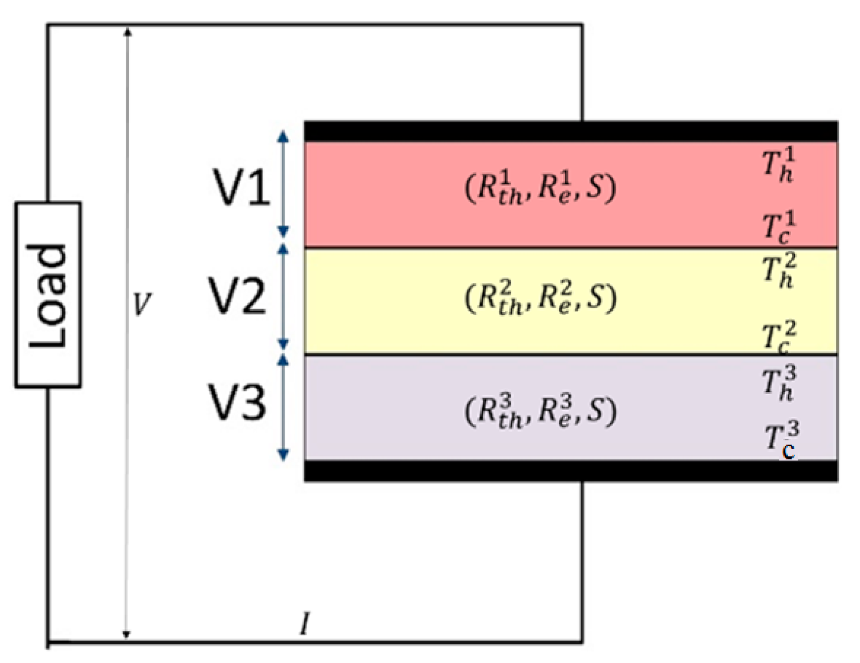
The input heat to solar absorber is the product of the collector surface and radiation intensity. The input energy and the absorbed heat are expressed as,

$${\dot{Q}}_H={\dot{Q}}_{Absorber}-{\dot{Q}}_{L,Rad}-{\dot{Q}}_{L,Cond}$$

(6)

$${\dot{Q}}_{Absorbe}=\tau ·\alpha ·{\dot{Q}}_{Solar}$$

(7)

$${\dot{Q}}_{Solar}={\dot{q}}_{Solar}·TC·A_{TEG}$$

(8)

The thermal losses can be expressed as:

$${\dot{Q}}_{L,Rad}=A_{coll}\epsilon ·{\sigma }_{SB}·\left[T_{absorber}^4-T_{amb}^4\right]$$

(9)

$${\dot{Q}}_{L,cond}=K_{enclose}\left[T_{absorber}-T_{amb}\right]$$

(10)

In the Simulink view, the solar absorber acts as a current source, controlled by absorber temperature, radiation intensity, and the system dynamic. The cold side was considered as a controllable voltage (temperature) source, and the electrical load block as a controllable resistor. In the case of maximum electrical efficiency, the load’s resistance should be equal to the TEG’s internal resistance.

2.3. TEG Model

Peltier’s, Seebeck’s, and Ohm’s laws are governing equations for TEG devices. By dividing TEG into stacked blocks, temperature-dependent material properties can be used. In this approach, the TEG is divided into several thin TEGs, which are thermally and electrically connected in series. The output of each block is an input for the next block. Due to only small temperature differences along each block, it is possible to assume that temperature is constant and use locally constant temperature-dependent materials’ properties. Figure 4 shows a schematic of this method.

The heat transfer and electrical equations in each block are,

$${{\dot{Q}}_h}^i=\left[S.I+{K_{th}}^i\right]\left[{T_h}^i-{T_c}^i\right]-V^{i}I$$

(11)

$$V^i=S\left[{T_h}^i-{T_c}^i\right]$$

(12)

$$I=\frac{V}{R_e+R_{Load}}$$

(13)

$$V={\displaystyle \sum }_{i=1}^{\mathrm{n}}{V}_i$$

(14)

$$R_e={\displaystyle \sum }_{i=1}^{\mathrm{n}}{R}_i$$

(15)

Properties of the blocks are computed based on average temperature of the block, number of the blocks and temperature dependent properties of the module can be expressed as:

$$R_e^i=\frac{R_e\left(T_i\right)}{{\displaystyle \sum }i}$$

(16)

$$K_{th}^i=\left[K_{th}\left(T_i\right)\right]·{\displaystyle \sum }i$$

(17)

TEG properties for different ZT values are presented in

Table 2. TEG temperature dependent properties in one verified (ZT = 0.8) and two (Z = 1.2 and ZT = 1.5) modified conditions.

Module Figure of Merit	${\mathit{A}}_{\mathit{s}}\left({10}^{-7}\right)$	${\mathit{B}}_{\mathit{s}}\left({10}^{-4}\right)$	${\mathit{C}}_{\mathit{s}}\left({10}^{-4}\right)$	${\mathit{A}}_{\mathit{R}}\left({10}^{-5}\right)$	${\mathit{B}}_{\mathit{R}}\left({10}^{-4}\right)$	${\mathit{C}}_{\mathit{R}}\left({10}^{-4}\right)$	${\mathit{A}}_{\mathit{t}\mathit{h}}\left({10}^{-4}\right)$	${\mathit{B}}_{\mathit{t}\mathit{h}}\left({10}^{-4}\right)$	${\mathit{C}}_{\mathit{t}\mathit{h}}$
$Z{T}_{max}=0.8$	$-2$	$2$	$4.4$	$5$	$141$	$4418$	$-2$		$-3.78$
$Z{T}_{max}=1.2$	$-2$	$2$	$5$	$5$	$136$	$4241$	$-2$		$-4.736$
ZTmax = 1.5	$-2$	$2$	$5.3$	$5$	$127$	$3976$	$-2$		$-4.903$
$S\left(T\right)=A_s{T}^2+B_{s}T$ + $C_s$ $R_e\left(T\right)=A_R{T}^2+B_{R}T+C_R$ $R_{th}\left(T\right)=A_{th}{T}^2+B_{th}T+C_{th}$			TEG dimensions (L × W × H) are $8.7\times 8.7\times 1.4 \left({\mathrm{mm}}^3\right)$.

. In Case #1 (ZT = 0.8), the coefficients were extracted by fitting curves for experimental data. Afterward, the coefficients were modified to make maximum ZT equal to 1.2 and 1.5 for Cases #2 and #3, respectively. In the present study, the value of the figure of merit refers to an effective ZT module [30].

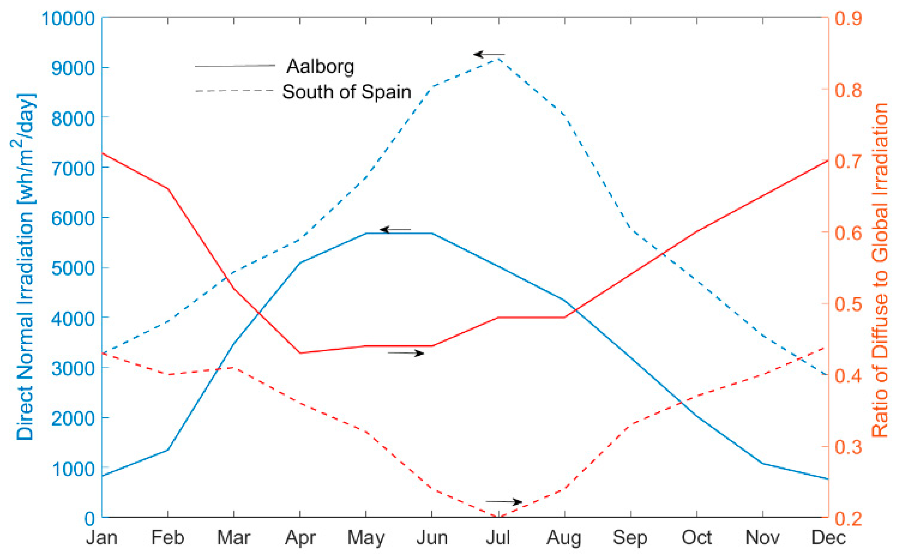
2.4. Meteorological Data

The Joint Research Centre, which is the commission’s science and knowledge service, provides an online database of environmental data related to renewable energies [25] exploited in this study. Two places in Europe with different insolation and temperature regimes were selected: Aalborg (57°2′11″ N, 9°55′21″ E) in the North of Denmark, which is mostly cloudy with diffused isolation and 7–18 daylight hours. The second location is Gibraltar (36°19′36″ N, 5°37′29″ E), which has more direct radiation and 10–14 daylight hours. This selection was based on a diffused to direct ratio of sun isolation (see Figure 1) in order to compare the STEG and concentrated CHP. The values of direct, diffused, and total irradiance in Aalborg and Gibraltar are shown in

Table 3. Yearly average of direct, diffused, and global irradiance in Aalborg and Gibraltar.

Location	$\mathbf{Direct}\left[\mathbf{W}.\mathbf{h}/{\mathbf{m}}^2\mathbf{d}\mathbf{a}\mathbf{y}\right]$	$\mathbf{Diffused}\left[\mathbf{W}.\mathbf{h}/{\mathbf{m}}^2\mathbf{d}\mathbf{a}\mathbf{y}\right]$	$\mathbf{Global}\left[\mathbf{W}.\mathbf{h}/{\mathbf{m}}^2\mathbf{d}\mathbf{a}\mathbf{y}\right]$
Aalborg	3220	3093	6313
Gibraltar	5050	2601	7651

, according to which the diffused irradiance in Aalborg was 19% higher compared to Gibraltar. However, global irradiance was 21% lower.

2.5. Optimization Process

The optimization process was mainly carried out to find the desired value of TC so that the maximum STEG performance could be obtained in a specific location in a year. The inputs are meteorological data, STEG performances curves (at different cold side temperatures and incident radiation), and maximum hot side temperature of the TEG, which is considered a limiting factor during the process. The pairs of maximum efficiency and correlated TC were calculated based on air temperature, solar insolation, and STEG curves. The weighted mean of $\mathrm{TC}\mathrm{and} \eta$ were the yearly optimal TC and efficiency of the system. The hot side temperature limitation was applied in the final step. TC increased discriminately to ensure that temperature is in the safe zone for the module. The maximum tolerable temperature is based on solder durability, For instance, it is considered between 400 and 450 K.

$$T{C}_{opt}=\frac{{\eta }_{1}T{C}_1{q}_{sol,1}+{\eta }_{2}T{C}_2{q}_{sol,2}+\cdots {\eta }_{n}T{C}_n{q}_{sol,n}}{{\eta }_1{q}_{sol,1}+{\eta }_2{q}_{sol,2}+\cdots +{\eta }_n{q}_{sol,n}}$$

(18)

$${\eta }_{opt}=\frac{{\eta }_1{q}_{sol,1}+{\eta }_2{q}_{sol,2}+\cdots {\eta }_n{q}_{sol,n}}{q_{sol,1}+q_{sol,2}+\cdots +q_{sol,n}}$$

(19)

Each point refers to 15 min of daylight. The weighted average (Equations (18) and (19)) gives the optimum values of TC and $\eta$ efficiency in the period of one year.

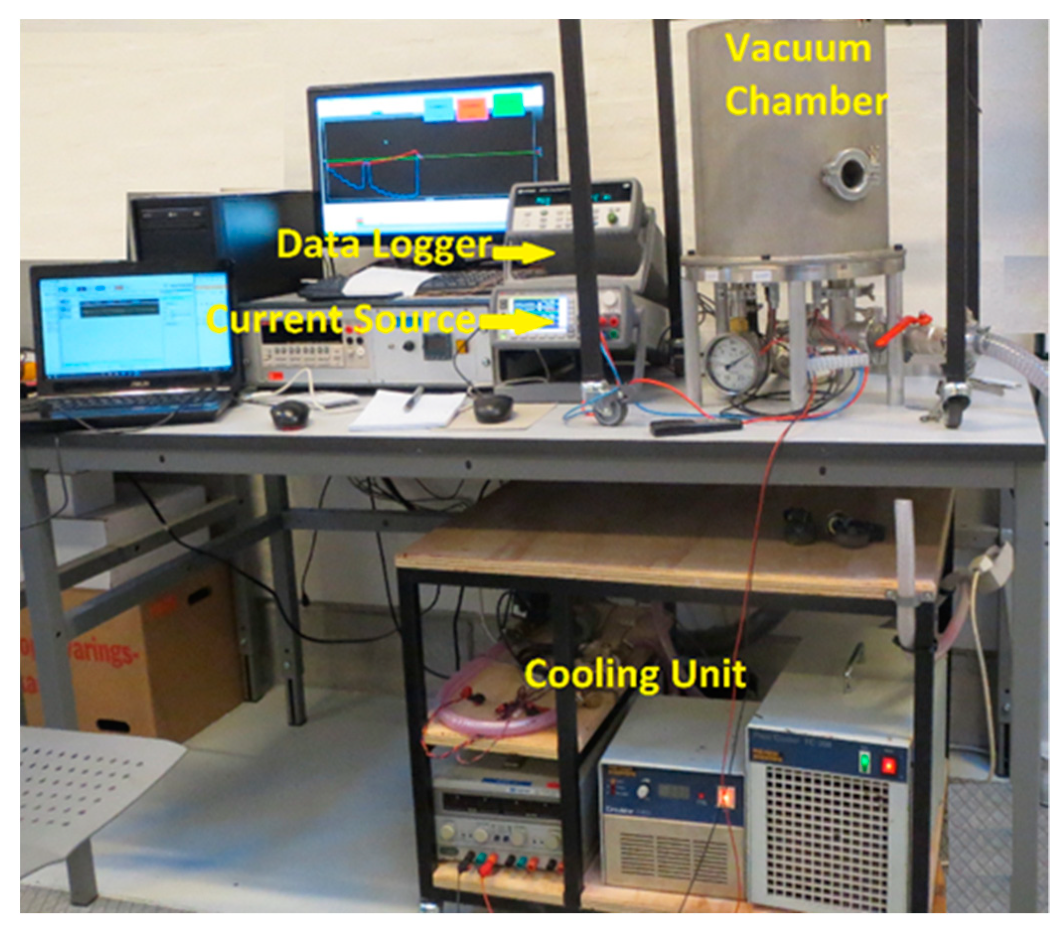
2.6. Experimental Setup

To obtain the module properties and validate the model, a sample module was tested by Tegeta at the Aalborg University [31]. This setup was designed initially to characterize high temperature oxide materials [31], and it was modified for the mid temperature module studied in this paper. Figure 5 shows the modified setup in which the ceramic heater is replaced by a ULTRAMIC 600 supplied with Keysight B2900 to maintain the hot side at the desired temperature. T-type thermocouples, with a diameter of 50 micrometers and a nominal response time of 20 milliseconds sense temperatures. The Keysight 34972 logged data every 10 s. The second channel of the Keysight B2900 was used to run constant reverse voltage and emulate the electrical load. Silicon thermal past is used between layers to ensure low thermal resistance between the hot side and TE module as well as the module and heat sink. The measurement was run over different temperatures, and all data was stored in a text file then imported to a Microsoft Excel spreadsheet for further analysis. The standard procedure to characterize TE modules was: set constant temperature and electrical load until thermal and electrical stability was achieved then log the corresponding data for each electrical load. The data was processed later to fit the output power versus electrical load. The corresponded electrical load of maximum output power is the internal electrical resistance of module.

3. Results and Discussion

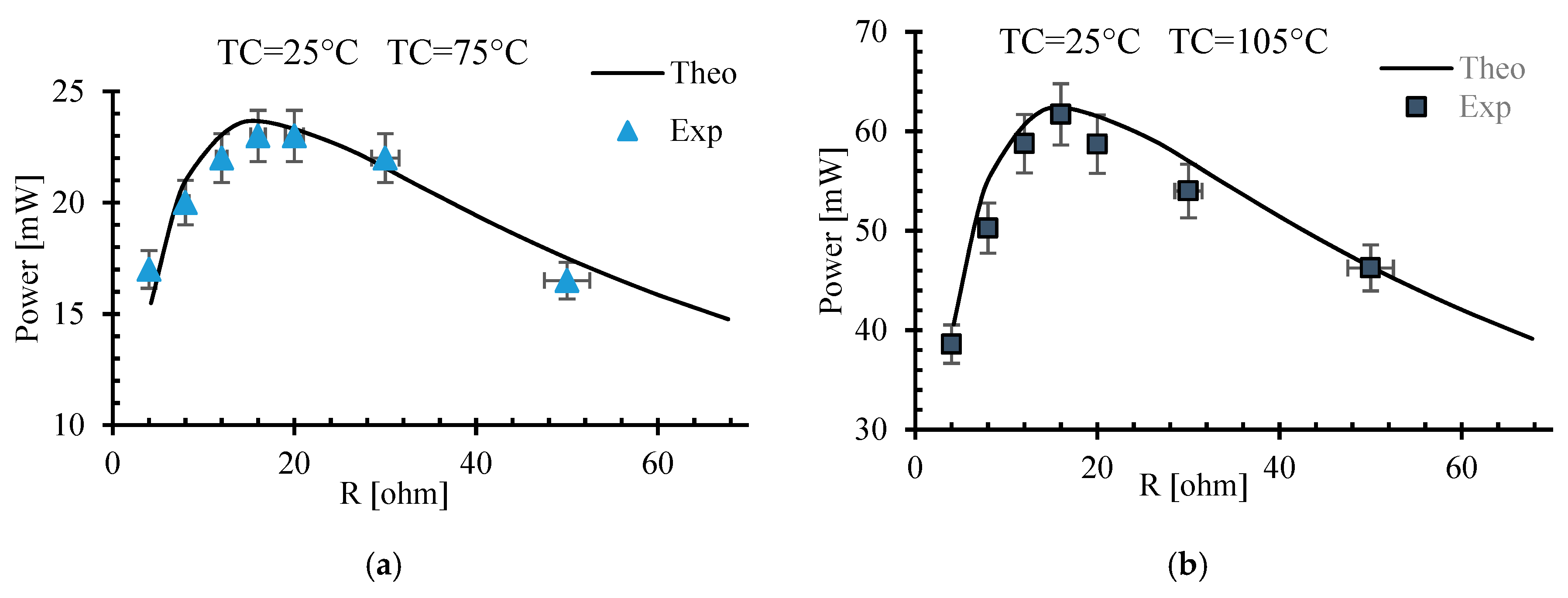
3.1. Experimental Validation of Simulink Model

Zmeter is a known method to characterize TE materials and modules; details can be found in previous papers [32,33]. The module properties were extracted by a series of experiments at different temperatures. Later, the obtained values of temperature, electrical voltage, current, and heat flow were used to fit curves, presented in Table 2. The nominal figure of merit for the tested module is 0.8; higher values can be produced by adjusting the data. Afterwards, the setup was used to validate the model. Predicted and measured values for the maximum power and corresponding electrical properties are presented in

Table 4. Comparison between measured and calculated values of matched electrical load and respected output power.

Cold Side	Temperature Difference	R [ohm]		P [mW/cm2]
		Measured	Calculated	Measured	Calculated
TC = 25 °C	dT = 15 °C	12.85	12.14	1.16	1.14
TC = 25 °C	dT = 20 °C	13.2	12.14	1.39	1.21
TC = 40 °C	dT = 15 °C	13.14	12.14	1.23	1.17
TC = 40 °C	dT = 20 °C	13.7	12.14	1.45	1.29

. The fill factor of the module was 0.7 and the number of thermocouples was 100. This module is designed to harvest energy in sensory systems.

Figure 6 shows the measured and calculated power module at two temperature differences between hot and cold sides. The mismatching between calculated and measured electrical resistance is due to sidewall thermal losses, and it is increased by increasing the average temperature, comparing between Figure 6a,b. However, the difference is acceptably less than 10 percent of the total power [34]. This proves that the model can represent a real system with an acceptable error.

3.2. Performance Curves of TE Module

The temperature distribution along the heat conduction direction in the TEG module is shown in Figure 7. Due to different heat transfer mechanisms, the temperature distribution along the TE elements is not linear. In order to have a faster simulation, the thermal mass of the solar collector was eliminated from the simulations. It is worth noting that the long response time of the TEGs is an advantage that causes higher stability in power generation systems, thereby diminishing the necessity of fast MPPT [35] algorithms and providing an intrinsic storage capability for the system. According to Table 2 and

Table 5. Thermal properties of thermoelectric materials and solar collector.

--	$\mathbf{Thermal}\mathbf{Conductivity}\left[\mathbf{W}/\mathbf{m}\mathbf{K}\right]$	$\mathbf{Heat}\mathbf{Capacity}\left[\mathbf{J}/\mathbf{g}\mathbf{K}\right]$	$\mathbf{Density}\left[\mathbf{g}/{c}{\mathbf{m}}^3\right]$
Copper	385	0.385	8.9
$\mathit{B}{\mathit{i}}_{\mathbf{2}}\mathit{T}{\mathit{e}}_{\mathbf{3}}$*	1.5	0.544	7.29

* The average value for n and p-type materials.

, the STEG time constant mostly depends on the solar thermal collector. For instance, a 1 $℃$ change in $500 \mathsf{\mu }\mathrm{m}$ thick copper takes 17 s when radiation is 1000 $\mathrm{W}/{\mathrm{m}}^2$.

Figure 8 exhibits the maximum STEG efficiency (a–c) and optimum TC (d–f) contours at different terrestrial conditions for various ZT values. Higher radiation intensity at constant cold side temperature increases the efficiency and decreases the corresponding TC, whereas an increase in the cold side temperature leads to a reduction in both efficiency and the corresponding TC, which is not a desirable condition. The opposite effects of air temperature and solar radiation intensity cause the relative efficiency in winter and summer days. For example, two different conditions in summer ($600\mathrm{W}/{\mathrm{m}}^2\mathrm{and}300\mathrm{K}$) and winter ($400\mathrm{W}/{\mathrm{m}}^2\mathrm{and}280\mathrm{K}$), have an equal efficiency of 4.8% for ZT = 0.8 and different values of TCs. Therefore, it is necessary to perform long-term optimization instead of only STC condition optimization. While the module with higher ZT increases efficiency, it simultaneously decreases TC. Incensement in ZT is due to the lower thermal conductivity of TE materials, which may lead to the manifestation of optimum temperature gradient at lower TC. For example, increasing ZT from 0.8 to 1.2 leads to the decrease of TCs at $200\mathrm{W}/{\mathrm{m}}^2$ and $500\mathrm{W}/{\mathrm{m}}^2$ by order of 200 and 110, respectively.

3.3. Optimization Results

Figure 9 and Figure 10 show how the optimum efficiency and TC can vary according to the terrestrial parameters, which confirms the necessity of yearly design optimization. Each blue dot in the figures refers to one data point. As observed, points with high values of TC were in early mornings or late evenings.

Table 6. The daily energy production in Aalborg and Gibraltar for different values of ZT compared with the parabolic trough.

Location	Parabolic trough [W. h/m2day]	ZT = 0.8 [W. h/m2day]	ZT = 1.2 $\left[\mathbf{W}.\mathbf{h}/{\mathbf{m}}^2\mathbf{d}\mathbf{a}\mathbf{y}\right]$	ZT = 1.5 $\left[\mathbf{W}.\mathbf{h}/{\mathbf{m}}^2\mathbf{d}\mathbf{a}\mathbf{y}\right]$
Aalborg	402	284	430	486
South of Spain	631	360	564	614

shows the daily energy production expectation for different values of ZT in comparison to the parabolic trough, which is a mature CHP technology with an average efficiency of 12.5% that can only capture DNI. Due to the higher amount of diffused radiation in Aalborg (49%), the increased ZT had more of an impact on energy production, compared to Gibraltar where diffused radiation is 33%. The parabolic trough can capture 67%of sun rays. STEG with ZT = 0.8 can generate 70% of the expected electrical power of the parabolic trough, and it could increase to 106% and 121% with ZT of 1.2 and 1.5, respectively.

In the second scenario, the dissipated heat on the cold side was the input to the heating system. This might cause a higher cold side temperature and lower total efficiency. Figure 11 shows the maximum efficiency and the corresponding TC for different cold side temperatures. The cold side temperature is assumed to be constant throughout a year, which is possible by control of the liquid flow and TEG current. The desirable water temperature of flat solar heat collectors was 320–350 K, which obtained efficiency between 3.5% and 2.5% for ZT = 0.8 in Aalborg. By increasing the ZT to 1.2, the efficiency increased to 6 and 4.5, respectively. The STEG efficiency in Gibraltar in the coproduction scenario was relatively higher compared to Aalborg. At lower water temperatures, this difference became more significant. By considering constant temperature for both locations, Aalborg lost the lower ambient air temperature merit. Compared to similar studies [19,36], where optimum TC varies between 120 and 270, the proposed model shows the significantly different values for TC. In the original study on STEG [19] it is between 180 and 220. Studying different materials by 3D simulations [36] shows the similar range for optimum TC. This is mainly due to the constant STC condition. The seasonal effect was studied previously [36] for two scenarios, winter and summer, and it is pointed out that the terrestrial condition significantly degrades STEG performance. Kossyvakis et al. [36] proposed to change the Fresnel lens or the focal point. A developed model represents an effort to overcome the seasonal effect by applying realistic data in the design step.

3.4. Controlling by Electric Current

According to the results, higher TC had better efficiency in the early morning and late noon due to higher energy flux. Meanwhile, lower TC provided more efficiency at noon because of lower heat losses. The results showed that the optimum point of TC was between these two values. There are two parameters with the ability to regulate the electricity generator and rejected heat at cold side: (i) electric current, which can be referred to as electrical load resistance, and (ii) cold side thermal resistance, which can be recognized as a volumetric flow of heat exchanger fluid. Due to the Peltier effect, the electric current variation exerts an impact on the thermal conduction. Figure 12 exhibits the variation of the load resistance from 0 (short circuit) to 80 ohms (open circuit), causing a 17.5% change in dissipated heat at the cold side of TEG. It means that when the solar radiation variation is below 17.5%, the water temperature can be regulated. Reversely, the output power can be kept constant by controlling the water flow of the heat exchanger.

4. Conclusions

There are several challenges in designing of thermoelectric generator systems mainly due to the several heat and electricity conversion mechanisms. The design of thermoelectric generator systems gets more complicated when dealing with an optimal design for terrestrial applications, which imposes more dynamic parameters to the system. STEGs have been designed and tested under standard test conditions based on the thermal concentration (TC) concept, showing the potential to reach energy conversion efficiency from sun rays to electricity above 4%. In this study, the new Simulink model to simulate STEGs under different conditions was presented and validated by experimental tests. The optimization results confirmed the necessity of long-term optimization. The optimum TC and maximum efficiency of STEG at two different realistic locations of Aalborg and Gibraltar were determined and the results showed that, in locations with a higher ratio of diffuse to direct radiation, STEGs could generate up to 70% of the energy of parabolic trough systems. This can increase by 106 to 121% using recently developed thermoelectric materials or cascade TEGs. The results demonstrated that the coupling between electrical and thermal flows provided the opportunity to control the temperature of cooling fluid and electrical power production. The flat-panel STEGs showed a greater number of advantages in locations with a higher ratio of diffuse to direct radiation. Considering promising new materials, which had higher ZTs and lower prices, STEGs could be more efficient even in single generation systems. In addition to the development of the materials, there are engineering challenges in this field, including the geometry of STEGs to provide uniform temperature at the hot and cold sides of the TEG, manufacturing challenges to provide maximum insolation between the hot and cold sides of the TEG, and the optimal STEG dimensions to achieve the greatest economic benefit.

References

1. Rowe, D. Applications of nuclear-powered thermoelectric generators in space. Appl. Energy 1991, 40, 241–271. [Google Scholar] [CrossRef]
2. Telkes, M. Solar thermoelectric generators. J. Appl. Phys. 1954, 25, 765–777. [Google Scholar] [CrossRef]
3. Hicks, L.; Dresselhaus, M. Effect of quantum-well structures on the thermoelectric figure of merit. Phys. Rev. B 1993, 47, 12727. [Google Scholar] [CrossRef]
4. Hicks, L.; Dresselhaus, M. Thermoelectric figure of merit of a one-dimensional conductor. Phys. Rev. B 1993, 47, 16631. [Google Scholar] [CrossRef]
5. Sokka, L.; Sinkko, T.; Holma, A.; Manninen, K.; Pasanen, K.; Rantala, M.; Leskinen, P. Environmental impacts of the national renewable energy targets—A case study from finland. Renew. Sustain. Energy Rev. 2016, 59, 1599–1610. [Google Scholar] [CrossRef]
6. Noppers, E.H.; Keizer, K.; Milovanovic, M.; Steg, L. The importance of instrumental, symbolic, and environmental attributes for the adoption of smart energy systems. Energy Policy 2016, 98, 12–18. [Google Scholar] [CrossRef] [Green Version]
7. Inglesi-Lotz, R. The impact of renewable energy consumption to economic growth: A panel data application. Energy Econ. 2016, 53, 58–63. [Google Scholar] [CrossRef] [Green Version]
8. Luque, A.; Hegedus, S. Handbook of Photovoltaic Science and Engineering; John Wiley & Sons: ‎Hoboken, NJ, USA, 2011. [Google Scholar]
9. Tian, Y.; Zhao, C.-Y. A review of solar collectors and thermal energy storage in solar thermal applications. Appl. Energy 2013, 104, 538–553. [Google Scholar] [CrossRef] [Green Version]
10. Cao, F.; McEnaney, K.; Chen, G.; Ren, Z. A review of cermet-based spectrally selective solar absorbers. Energy Environ. Sci. 2014, 7, 1615–1627. [Google Scholar] [CrossRef] [Green Version]
11. Kumar, R.; Rosen, M.A. A critical review of photovoltaic–thermal solar collectors for air heating. Appl. Energy 2011, 88, 3603–3614. [Google Scholar] [CrossRef]
12. Zhang, H.; Baeyens, J.; Degrève, J.; Cacères, G. Concentrated solar power plants: Review and design methodology. Renew. Sustain. Energy Rev. 2013, 22, 466–481. [Google Scholar] [CrossRef]
13. Müller-Steinhagen, H.; Trieb, F. Concentrating solar power. Ingenia Inform. QR Acad. Eng. 2004, 18, 43–50. [Google Scholar]
14. Chen, W.-H.; Wu, P.-H.; Lin, Y.-L. Performance optimization of thermoelectric generators designed by multi-objective genetic algorithm. Appl. Energy 2018, 209, 211–223. [Google Scholar] [CrossRef]
15. Olsen, M.; Warren, E.; Parilla, P.; Toberer, E.; Kennedy, C.; Snyder, G.; Firdosy, S.; Nesmith, B.; Zakutayev, A.; Goodrich, A. A high-temperature, high-efficiency solar thermoelectric generator prototype. Energy Procedia 2014, 49, 1460–1469. [Google Scholar] [CrossRef]
16. Kraemer, D.; Jie, Q.; McEnaney, K.; Cao, F.; Liu, W.; Weinstein, L.A.; Loomis, J.; Ren, Z.; Chen, G. Concentrating solar thermoelectric generators with a peak efficiency of 7.4%. Nat. Energy 2016, 1, 16153. [Google Scholar] [CrossRef] [Green Version]
17. Fuschillo, N.; Gibson, R.; Eggleston, F.; Epstein, J. Solar thermoelectric generator for near-earth space applications. IEEE Trans. Electron Devices 1966, 13, 426–432. [Google Scholar] [CrossRef]
18. Goldsmid, H.; Giutronich, J.; Kaila, M. Solar thermoelectric generation using bismuth telluride alloys. Sol. Energy 1980, 24, 435–440. [Google Scholar] [CrossRef]
19. Kraemer, D.; Poudel, B.; Feng, H.-P.; Caylor, J.C.; Yu, B.; Yan, X.; Ma, Y.; Wang, X.; Wang, D.; Muto, A. High-performance flat-panel solar thermoelectric generators with high thermal concentration. Nat. Mater. 2011, 10, 532–538. [Google Scholar] [CrossRef] [PubMed]
20. Lv, S.; He, W.; Hu, D.; Zhu, J.; Li, G.; Chen, H.; Liu, M. Study on a high-performance solar thermoelectric system for combined heat and power. Energy Convers. Manag. 2017, 143, 459–469. [Google Scholar] [CrossRef]
21. Sun, D.; Shen, L.; Yao, Y.; Chen, H.; Jin, S.; He, H. The real-time study of solar thermoelectric generator. Appl. Therm. Eng. 2017, 119, 347–359. [Google Scholar] [CrossRef]
22. Joshi, G.; Lee, H.; Lan, Y.; Wang, X.; Zhu, G.; Wang, D.; Gould, R.W.; Cuff, D.C.; Tang, M.Y.; Dresselhaus, M.S. Enhanced thermoelectric figure-of-merit in nanostructured p-type silicon germanium bulk alloys. Nano Lett. 2008, 8, 4670–4674. [Google Scholar] [CrossRef] [PubMed]
23. Chen, G. Theoretical efficiency of solar thermoelectric energy generators. J. Appl. Phys. 2011, 109, 104908. [Google Scholar] [CrossRef]
24. Kraemer, D.; McEnaney, K.; Chiesa, M.; Chen, G. Modeling and optimization of solar thermoelectric generators for terrestrial applications. Sol. Energy 2012, 86, 1338–1350. [Google Scholar] [CrossRef] [Green Version]
25. Photovoltaic Geographical Information System—Interactive Maps. Available online: http://re.jrc.ec.europa.eu (accessed on 14 June 2017).
26. Mitrani, D.; Tomé, J.A.; Salazar, J.; Turó, A.; García, M.J.; Chávez, J.A. Methodology for extracting thermoelectric module parameters. IEEE Trans. Instrum. Meas. 2005, 54, 1548–1552. [Google Scholar] [CrossRef]
27. Dalola, S.; Ferrari, M.; Ferrari, V.; Guizzetti, M.; Marioli, D.; Taroni, A. Characterization of thermoelectric modules for powering autonomous sensors. IEEE Trans. Instrum. Meas. 2009, 58, 99–107. [Google Scholar] [CrossRef]
28. Phillip, N.; Maganga, O.; Burnham, K.J.; Dunn, J.; Rouaud, C.; Ellis, M.A.; Robinson, S. Modelling and Simulation of a Thermoelectric Generator for Waste Heat Energy Recovery in Low Carbon Vehicles. In Proceedings of the 2012 2nd International Symposium on Environment Friendly Energies and Applications, Newcastle upon Tyne, UK, 25–27 June 2012. [Google Scholar]
29. Kane, A.; Verma, V.; Singh, B. Temperature Dependent Analysis of Thermoelectric Module Using Matlab/Simulink. In Proceedings of the 2012 IEEE International Conference on Power and Energy (PECon), Kota Kinabalu, Malaysia, 2–5 December 2012. [Google Scholar]
30. Kim, H.S.; Liu, W.; Chen, G.; Chu, C.-W.; Ren, Z. Relationship between thermoelectric figure of merit and energy conversion efficiency. Proc. Natl. Acad. Sci. USA 2015, 112, 8205–8210. [Google Scholar] [CrossRef] [PubMed] [Green Version]
31. Man, E.A.; Schaltz, E.; Rosendahl, L.; Kolaei, A.R.; Platzek, D. Experimental characterization procedure of thermoelectric generator modules under non-equilibrium thermal conditions. In Proceedings of the 2014 International Conference on Thermoelectrics, Nashville, TN, USA, 6–10 July 2014. [Google Scholar]
32. Amatya, R.; Mayer, P.; Ram, R. High temperature z-meter setup for characterizing thermoelectric material under large temperature gradient. Rev. Sci. Instrum. 2012, 83, 075117. [Google Scholar] [CrossRef] [PubMed]
33. Ando Junior, O.; Calderon, N.; de Souza, S. Characterization of a thermoelectric generator (teg) system for waste heat recovery. Energies 2018, 11, 1555. [Google Scholar] [CrossRef]
34. Shakouri, A. Recent developments in semiconductor thermoelectric physics and materials. Annu. Rev. Mater. Res. 2011, 41, 399–431. [Google Scholar] [CrossRef]
35. Dalala, Z.; Saadeh, O.; Bdour, M.; Zahid, Z. A new maximum power point tracking (mppt) algorithm for thermoelectric generators with reduced voltage sensors count control. Energies 2018, 11, 1826. [Google Scholar] [CrossRef]
36. Kossyvakis, D.; Vossou, C.; Provatidis, C.; Hristoforou, E. Computational analysis and performance optimization of a solar thermoelectric generator. Renew. Energy 2015, 81, 150–161. [Google Scholar] [CrossRef]
Figure 1. Direct normal irradiation and the ratio between diffused and global irradiation of two different places in Europe with different annual direct irradiance ( 2046   kWm 2 year 1 in Gibraltar and 1157   kWm 2 year 1 in Aalborg) [25].
Energies 11 02425 g001
Figure 2. Schematic of the studied Solar Thermoelectric Generator (STEG) designs. (a) Energy flow diagram in the system; (b) electric power generation; (c) heat and electricity cogeneration.
Energies 11 02425 g002
Figure 3. First level of STEG Simulink. Solar absorber, TEG, cold side, and load are four masked parts of a STEG system. The TC and cold side temperature can be fed from the Matlab workspace while other parameters are set inside the simulink.
Energies 11 02425 g003
Figure 4. A schematic of the dividing thermoelectric generators (TEG) into stacked layers. Each block has a Seebeck coefficient, and an electrical and thermal resistance corresponding to its average temperature.
Energies 11 02425 g004
Figure 5. Experimental setup to study the transient behavior of the thermoelectric generator.
Energies 11 02425 g005
Figure 6. Experimental results and model prediction for module power output. (a) Small temperature difference and (b) high temperature difference.
Energies 11 02425 g006
Figure 7. The temperature distribution along TEG legs.
Energies 11 02425 g007
Figure 8. (ac) Efficiency contours for different TEG properties according to cold side temperature and solar radiation intensity. (df) Optimum thermal concentration for different TEG properties according to cold side temperature and solar radiation intensity. In the case where ZT, cold side temperature, and radiation are 0.8, 300 K, and 300 W / m 2 , respectively, the optimum TC is 750 and the maximum efficiency is 3.8%.
Energies 11 02425 g008
Figure 9. Maximum efficiency and optimum TC in Aalborg. Black lines are the weighted averages for each year and the blue dots are the value for each point. X axes are data points, each point represents 15 min of sunshine.
Energies 11 02425 g009
Figure 10. Maximum efficiency and optimum TC in Gibraltar. Black lines are the weighted average for a year and blue dots are the value for each point. X axes are data points, each point represents 15 min of sunshine.
Energies 11 02425 g010
Figure 11. Maximum efficiency and corresponded TC for different values of ZT (ac) in the case where cold side temperature is constant.
Energies 11 02425 g011
Figure 12. The effect of electrical load and thermal resistance of cold side on dissipated heat at cold side.
Energies 11 02425 g012