Digital Adaptive Hysteresis Current Control for Multi-Functional Inverters


Internet of Energy Laboratory, Department of Technology Management for Innovation, The University of Tokyo, Tokyo 113-8656, Japan
*
Author to whom correspondence should be addressed.
Energies 2018, 11(9), 2422; https://doi.org/10.3390/en11092422
Submission received: 2 September 2018
/
Revised: 8 September 2018
/
Accepted: 12 September 2018
/
Published: 13 September 2018
(This article belongs to the Special Issue Control in Power Electronics)
Abstract
:This paper proposes a digital adaptive hysteresis current control method for multi-functional inverters in a power-flow control device called digital grid router. Each inverter can be controlled in master, grid-connected, or stand-alone modes, which can be specified by the controller. While the popular linear sine-triangle pulse width modulation (SPWM) control technique requires complicated proportional-integral (PI) regulators with an unavoidable time delay, hysteresis current control has a simple structure, fast responses, and robustness due to its independent system of parameters. Since the hysteresis current control method controls the output current stay around the reference current directly, in the multi-functional inverter, the reference output is not given by a current directly. Thus, the reference current used to implement the hysteresis current control in this study is calculated from the given reference voltage or power in each control mode. The controller uses high-speed sampled data at MHz level and is implemented by using a field-programmable gate array (FPGA). Experimental results show good performances of the proposed controller in controlling power exchanges in the digital grid router.
1. Introduction
Nowadays, distributed energy resources have become a solution to address energy security concerns, quality of power grids, and greenhouse gas emission standards in most countries [1,2]. The power grid has been developed with various distributed small sources, such as fuel turbines, gas, diesel, and renewable energy generations including photovoltaic, wind turbine, etc. However, these distributed generations cause problems such as voltage rise and instability problems in the power grid. The interconnection between these sources may increase the risk of cascading failures because any imbalance in the power grid may propagate quickly over a wide area [3,4]. Furthermore, it is difficult for the conventional grid architecture to maintain the supply-demand balance with the variations caused by the increase of renewable and variable energy generations [5,6].
In order to accept more and more renewable energy by enhancing the reliability of the conventional power grid, a concept called digital grid has been proposed [6]. In the digital grid system, the large scale synchronized current power system is divided into multiple smaller power systems called digital grid cells. The digital grid cells are connected together and connected to the current grid asynchronously via a digital grid router (DGR). The DGR identified by its media access control (MAC) address can send power packets to any location over existing transmission lines or by using other sub-grids with a peer-to-peer power network.
The DGR is composed of multiple AC/DC/AC multi-functional inverters connecting to a common DC bus. This structure allows the DGR to transmit the power-packets between the various distributed electrical sources, the load, and the power grid asynchronously. The functions of each inverter are changed just by the control algorithm, regardless of the inverter circuit. Thus, the controller for each inverter in the DGR plays an important role in accommodating router legs with electrical power.
Among various current control techniques for inverters, the hysteresis current control technique is used in many applications of switching inverters due to its simplicity in implementation. The popular linear sine-triangle pulse width modulation (SPWM) technique has a disadvantage of requiring a complicated proportional-integral (PI) regulator with an unavoidable delay. On the other hand, hysteresis current control has fast responses and robustness due to its independent of system parameters [7,8]. The switching signals of the hysteresis current control are derived by comparing the actual hysteresis current with the reference current bounded by a band. In the classical hysteresis control technique, the hysteresis current band is fixed to a certain value. This makes the switching frequency vary to retain the hysteresis current within the hysteresis current band and leads to unwanted resonance in the output current [9]. In order to solve this problem, an adaptive hysteresis current control, which has the hysteresis current band controlled adaptively to maintain the switching frequency at a constant value, has been proposed. In the adaptive hysteresis current control, the hysteresis current band is not fixed at a constant value but calculated using the measured output voltage during each switching modulation period [10,11].
Since a digital controller usually requires an efficient high sampling frequency at MHz level to control the hysteresis current with an accurate switching time, it is difficult to implement the hysteresis current control on a conventional microcomputer or digital signal processor (DSP), which have the sampling frequency at kHz level [12,13]. However, calculations for such the high sampling frequency can be implemented on a high-speed field programmable gate array (FPGA), which is being used in more and more applications of the inverter control. In this study, we propose a control method for the multi-functional inverter in the DGR using FPGA-based digital adaptive hysteresis current control.
This paper is organized as follows: the concepts of the digital grid system and digital grid router are introduced in Section 2. The adaptive hysteresis current control method is presented in Section 3. The adaptive hysteresis current control for multi-functional inverters is proposed in Section 4. The experimental results showing the good performances of the proposed control method are in Section 5. Conclusions are presented in Section 6.
2. Digital Grid and Digital Grid Router
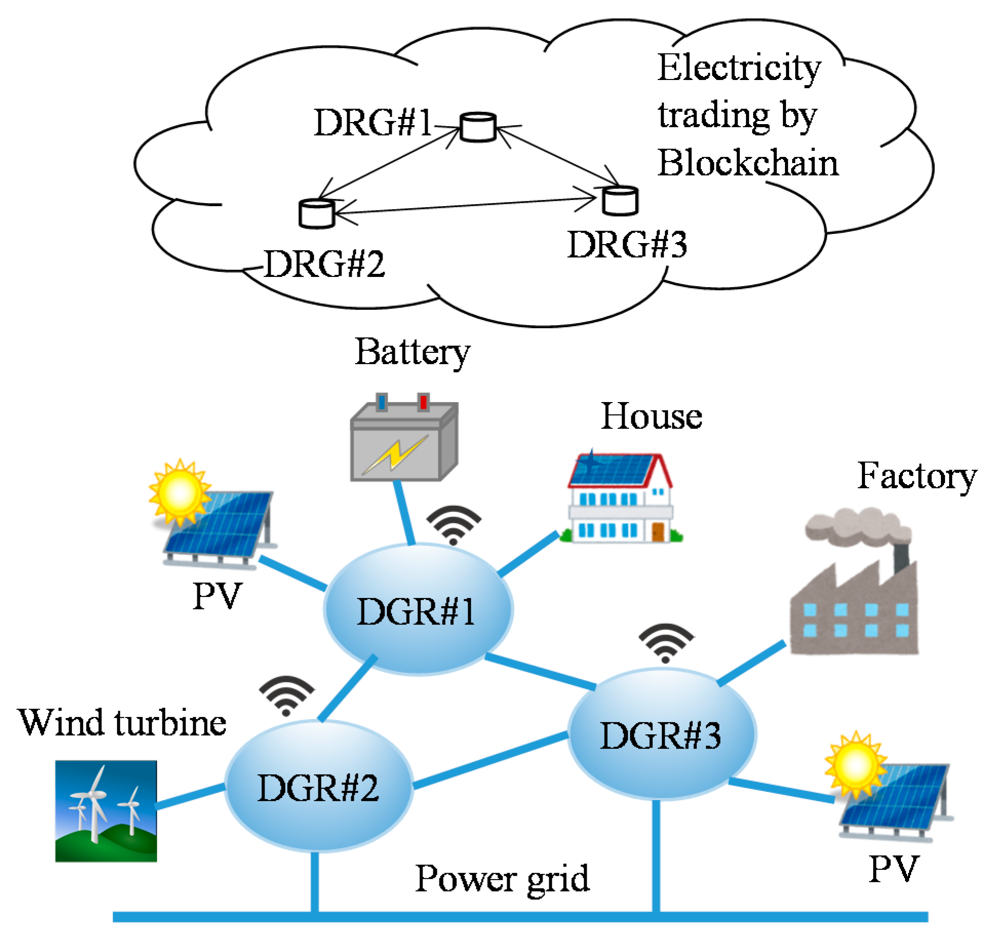
The conception of the digital grid system is dividing the large scale synchronized current power system into multiple smaller asynchronous digital grid cells connecting to the current main grid, to each other, and to other power sources using the power routers DGR as shown in Figure 1 [14]. The DGR receives the electrical trading results from the trading system and control the power flow between the equipment connecting to the cell. The renewable energy sources controlled by the DGR generate powers based on the electrical trading results so that their effects on the main grid can be increased. The stability of the main grid also can be supported by the energy storages such as batteries in the digital grid cells. The DGR is composed of multi-functional inverters connected to an internal DC bus, which is controlled at a constant voltage by one of the connected inverter. A software-based digital controller enables the multi-functional inverter to connect to various power sources within the cell or connect to other cells via a sub-grid flexibility.
The Japanese power grid can be considered as an example for the digital grid concept. The Japanese grid is composed of three independent power grids connected by two AC/DC/AC power conversion stations. The peak demand of the North, East, and West grids are 5.4 GW, 113 GW, and 66 GW respectively. The capacity of the power conversion station between the North and the East grids is 0.6 GW, and the one between the East and the West grids is 1 GW. The North and the East grids have their frequency at 50 Hz, while the West grid has its frequency at 60 Hz [15]. The digital grid concept can also be adapted to US or Europe regions, which are composed of various asynchronous grids that are similar to the case of Japan.
The electrical trading in the digital grid system is based on the demand and supply of the users, which are predicted by the trading system. The states of all power sources and loads connecting to the DGR are sent to the trading system on the cloud by using a communication networks such as Wi-Fi or 4G network. The transactions of the electrical trading system can be implemented automatically using the smart-contracts, an application of the block-chain technology. The trading strategy can be specified by the users and be implemented by a price-matching algorithm likes the Zaraba method [16] used in stock markets. The digital grid system composed of the power flow controller DGR and the autonomous trading system is expected to yield a free market with various players and enhance the power grid under the instability caused by the peak-demand cutting and demand-response matching issues.
The remaining parts of this paper will focus on the method to control the multi-functional inverters in the DGR.
3. Adaptive Hysteresis Current Control
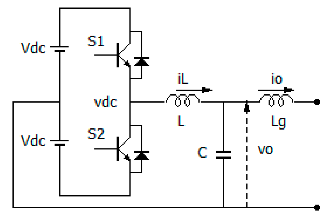
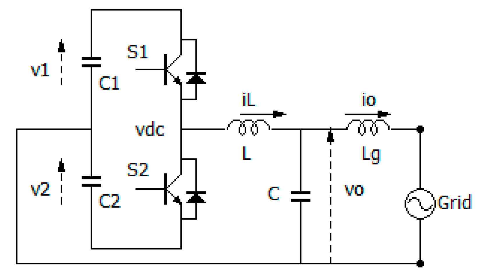
Consider a half-bridge inverter circuit, which has two constant and balanced DC sources as shown in Figure 2. Each of the DC sources has a voltage of . Parameters , , and represent the capacitance of the hysteresis current filter, the output inductance, and the grid-connected inductance, respectively. Assume that the output current of the inverter needs to be controlled to track a specified reference current . The digital controller uses data from voltage and current sensors sent through analog/digital converters to calculate the on/off pulses of the switches and .
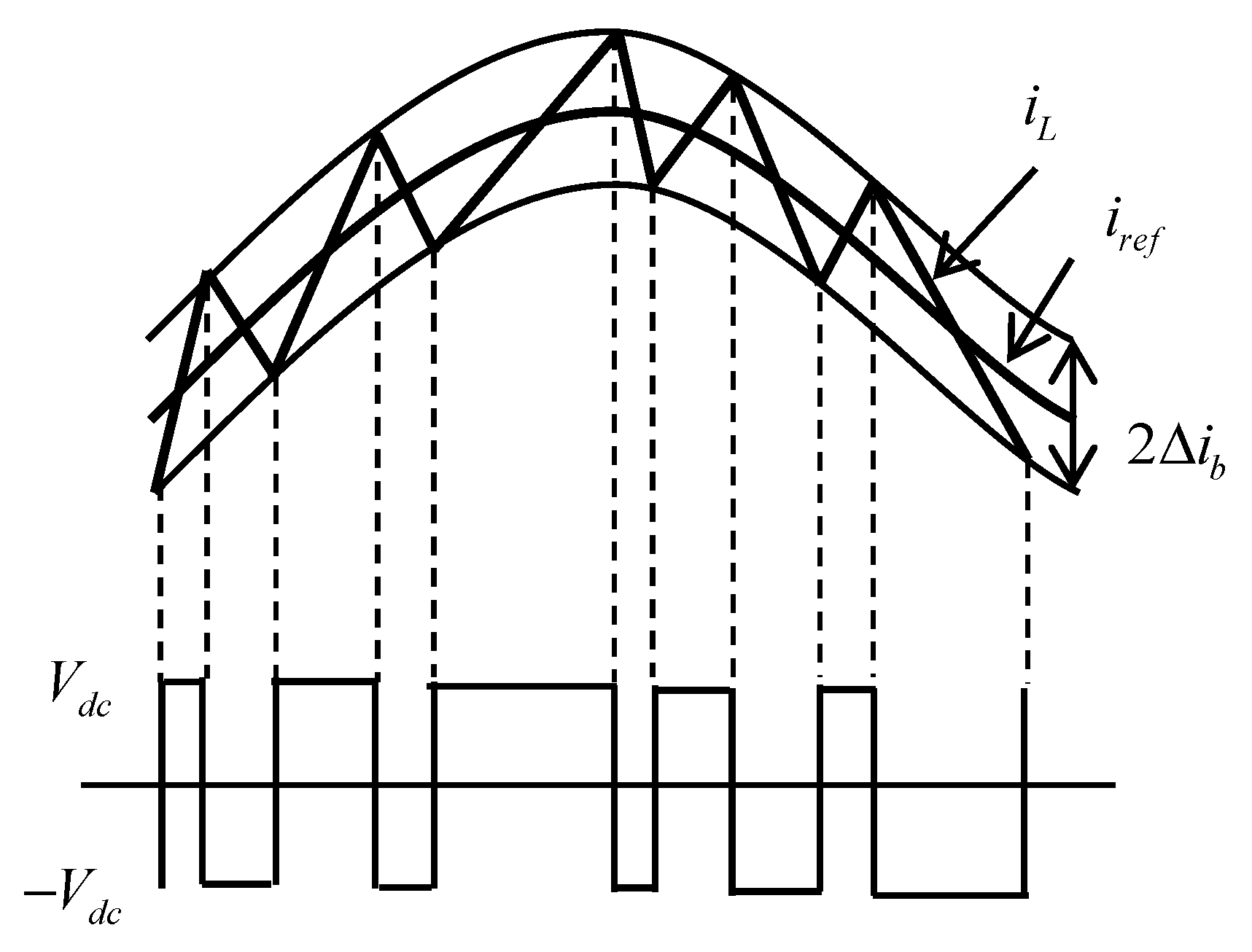
In the classical hysteresis current control technique, the hysteresis current band is usually fixed to a certain value . While the actual hysteresis current is within the hysteresis current band, states of the switches are unchanged. When the hysteresis current is equal to or greater than the upper limit of the current band , the switch is turned off and the switch is turned on to decrease the hysteresis current. In contrast, when the hysteresis current is equal to or less than the lower limit of the current band , the switch is turned on, the switch is turned off and the hysteresis current is increased to come back into the current band, as seen in Figure 3 [17].
Remark 1.
The ripple component of the hysteresis current in Figure 3 is filtered by the ripple current filter . As a result of this filter, the output current can track the reference current without the ripple component.
As mentioned in the introduction session, the fixed band hysteresis current control technique has many advantages in fast and stable response, simplicity, and independent of system parameters. However, a drawback of this technique is the non-constant switching frequency, that may lead to unwanted heavy interferences [18]. The adaptive hysteresis current control technique, which can achieve the constant switching frequency, has been presented in the pieces of literature [19,20,21]. The hysteresis current band in this technique is calculated adaptively using the measured output voltage and the desired constant switching frequency as:
where is the constant switching frequency. The reference current is slowly varying during the modulation period, such that the hysteresis current band in Equation (1) can be approximated as:
For digital control systems, where the voltage and current are sampled by analog/digital converters (ADCs), the hysteresis current band in Equation (2) under zero-order-holds (ZOHs) can be written by:
where , and is a sampling interval.
4. Hysteresis Current Control for Multi-Functional Inverter
In this work, the adaptive hysteresis current control is used to control the multi-functional inverters composing the DGR. In the hysteresis current control method, the hysteresis current is controlled to stay in a tolerance band around the reference current directly. However, in multi-functional inverters, the reference output is not given by a reference current directly, but by a reference voltage or power. Thus, we need to calculate the reference current from the given voltage or power. The reference currents for the three main modes of the multi-functional inverter used in the DGR: stand-alone, grid-connected, and master modes, are calculated as below.
4.1. Stand-Alone Mode
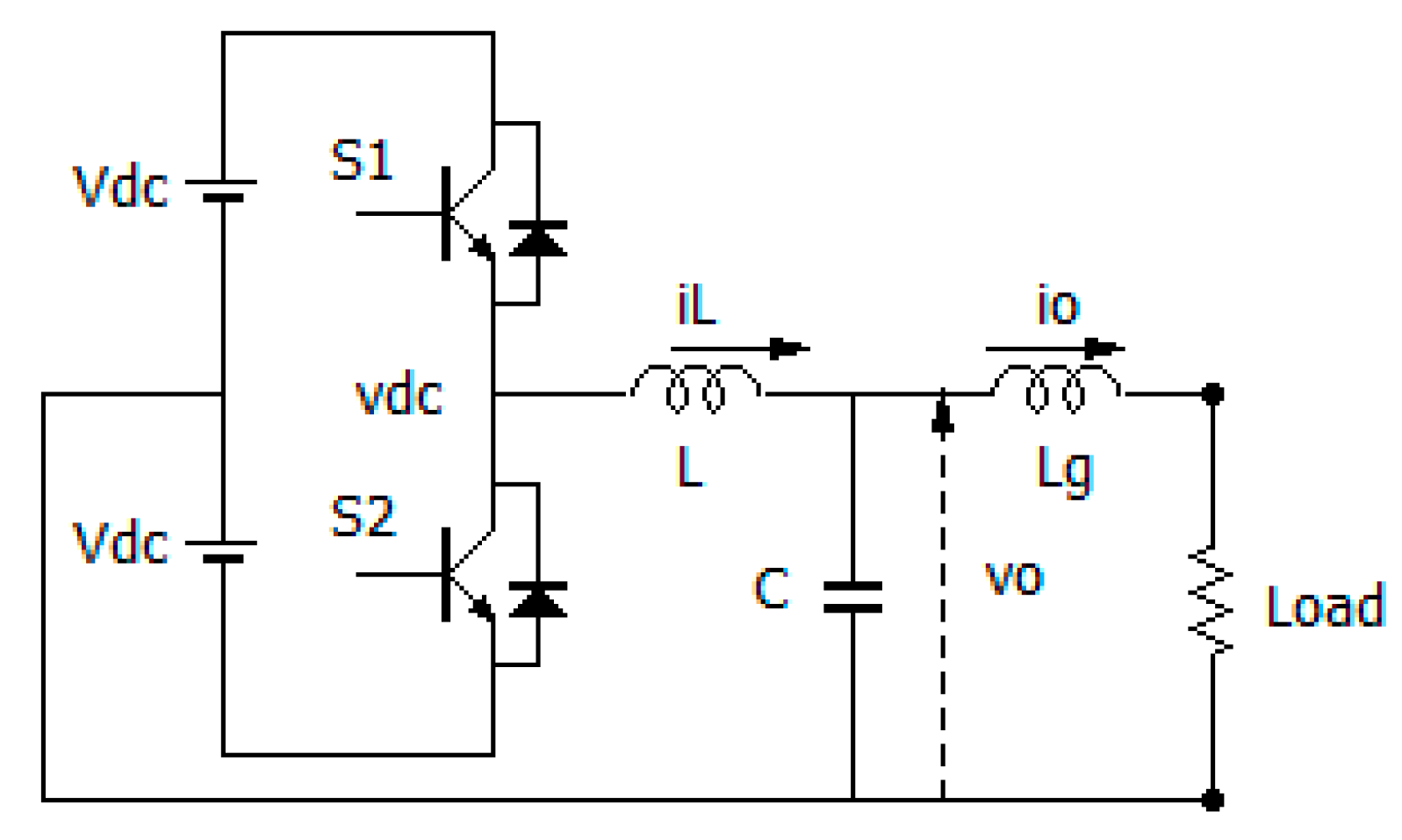
In stand-alone mode, the inverter is unconnected to the grid as shown in Figure 4. The inverter receives electrical power from the DC sources to supply a given reference output voltage for a load. This reference voltage may be an AC or DC voltage.
Using the mind of the hysteresis current control, one may think the hysteresis voltage control algorithm, where the switches are controlled comparing the output voltage with tolerance voltage bands directly, to control the output voltage track to a given reference voltage . However, comparing with the linear response of the current, the voltage responses to the switching modulation too slowly. It makes the ripple voltage cross over the hysteresis voltage bands and the switching frequency is difficult to be controlled [22].
In this work, the hysteresis current control technique is applied to control the output voltage of the inverter indirectly. The reference current used for hysteresis current control can be calculated from the given reference voltage is as below.
Using the Kirchhoff's circuit laws for the circuit as shown in Figure 4, we can calculate the reference current flows through the output inductance at the sampled-instant by a sum of the output current and the ripple current as:
The ripple current is conducted by the difference between the measured output voltage and the reference output voltage in each switching period as the following equation:
Thus, the reference current used for hysteresis current control can be derived by:
Then, the output voltage is controlled to track the reference voltage indirectly by using the hysteresis current control technique with the reference current and the hysteresis current band given by Equations (6) and (3) respectively.
4.2. Grid-Connected Mode
In the grid-connected mode, the output of the inverter is connected to the grid directly as shown in Figure 5. The inverter converts a given electrical power from the DC sources into AC power and supplies it to the grid.
When the given power is positive, the grid receives power from the inverter. In contrast, when the given power is negative, the DC sources receive power from the grid. An important point in the grid-connected mode is that the output current is controlled so that it is in phase with the grid voltage to maximize the power efficiency. Thus, the output current of the inverter requires a fast dynamic response to cope with the requirement of power delivery.
Assume that the grid voltage at a sampled-instant is given by:
where is effective value and is phase angle of the grid voltage. Then the effective value of the reference current can be calculated by:
The reference current needs to be in phase with the grid voltage, then it can be written as:
Multiplying the denominator and numerator of the right-hand side of Equation (9) by , and using Equation (7), we can write the reference current as:
In the conventional sine-triangle PWM method, the output voltage is synchronized with the grid voltage by using the phase lock loop (PLL) tool to calculate the phase angle of the grid voltage. The PLL method is basically using the analog circuit to find the zero crossing point, which may be inappropriate with the digital control where the datum is sampled by the AD converters. In this work, the inverter can supply a given power with the output current is in phase with the grid voltage by using hysteresis current control, where the reference current given by Equation (10), without the complicated PI regulator and PLL tool [23].
4.3. Master Mode
In the stand-alone and grid-connected modes, the inverters convert the DC power from the DC sources to the AC power and supply it to the load or the grid. These operation modes are also called slave modes. On the other hand, in the master mode, the inverter receives the AC power from the grid to maintain the voltages of the DC bus, which is composed of electrolytic capacitors at a given constant value as shown in Figure 6. This voltage is considered as the DC power supplier for the other inverters operated in the slave mode in the DGR. The power sent by the inverter operated in the master mode to the DC bus equals the power received by the inverters operated in the slave mode.
Assume that the inverter is controlled to maintain the voltages , of the capacitors and at a constant value of . Literatures [24,25] show that if the voltages and are controlled separately, or the sum voltage is controlled singularly, it may lead to an unbalance between the voltages , . As a result, it may lead to the unbalance of DC sources from the view of the slave inverters. A number of control methods have been proposed to balance these voltages [26,27]. However, most of them are for the conventional sine-triangle PWM control. In this work, the hysteresis current control for controlling the voltages of these two electrolytic capacitors is proposed as below.
Let the grid voltage be given by Equation (7). The reference current in the hysteresis current control can be calculated as:
where are the control gains, which tune the speed of the response. The first term of the reference current in Equation (11) controls the total voltage of the DC bus while the second term balances the two separate voltages and simultaneously. When the total voltage , the capacitors are charged by the passive power, and when the total voltage , the capacitors are discharged by the active power of the inverter. Additionally, when the voltage is higher than , it is decreased by the positive DC component of the output current. On the contrary, when the voltage is higher than , it is decreased by the negative DC component of the output current.
Remark 2.
The master-slave control for paralleled inverters [28] can be implemented by combining the proposed stand-alone and grid-connected control modes. The stand-alone inverter plays as the master to produce a reference voltage. The other grid-connected inverters connect to the master and play as slaves.
5. Experimental Results
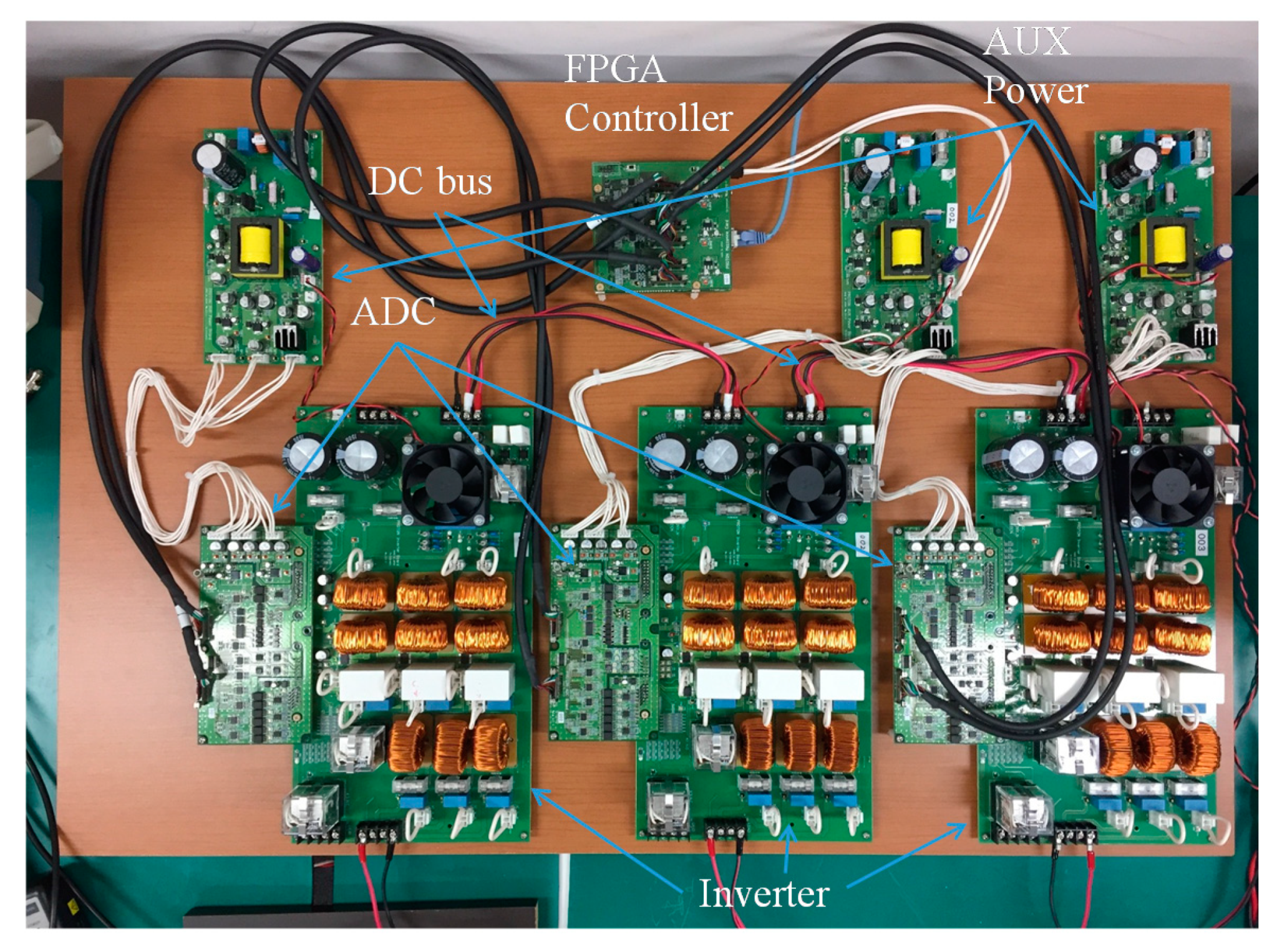
The proposed control algorithm has been assessed by using a prototype of the DGR composing of three inverters as shown in Figure 7. Each inverter in the DGR has a rated power of 300 W. The inverter circuit has the parameters given by: , , and . The analog/digital converter (ADC) has the sampling frequency of 4 MHz and the output data is at 12 bit. The constant switching frequency in the adaptive hysteresis current control is at 20 kHz. The proposed control algorithm is implemented on an FPGA-based digital controller, which is used with the clock frequency of 160 MHz.
5.1. Stand-Alone Mode
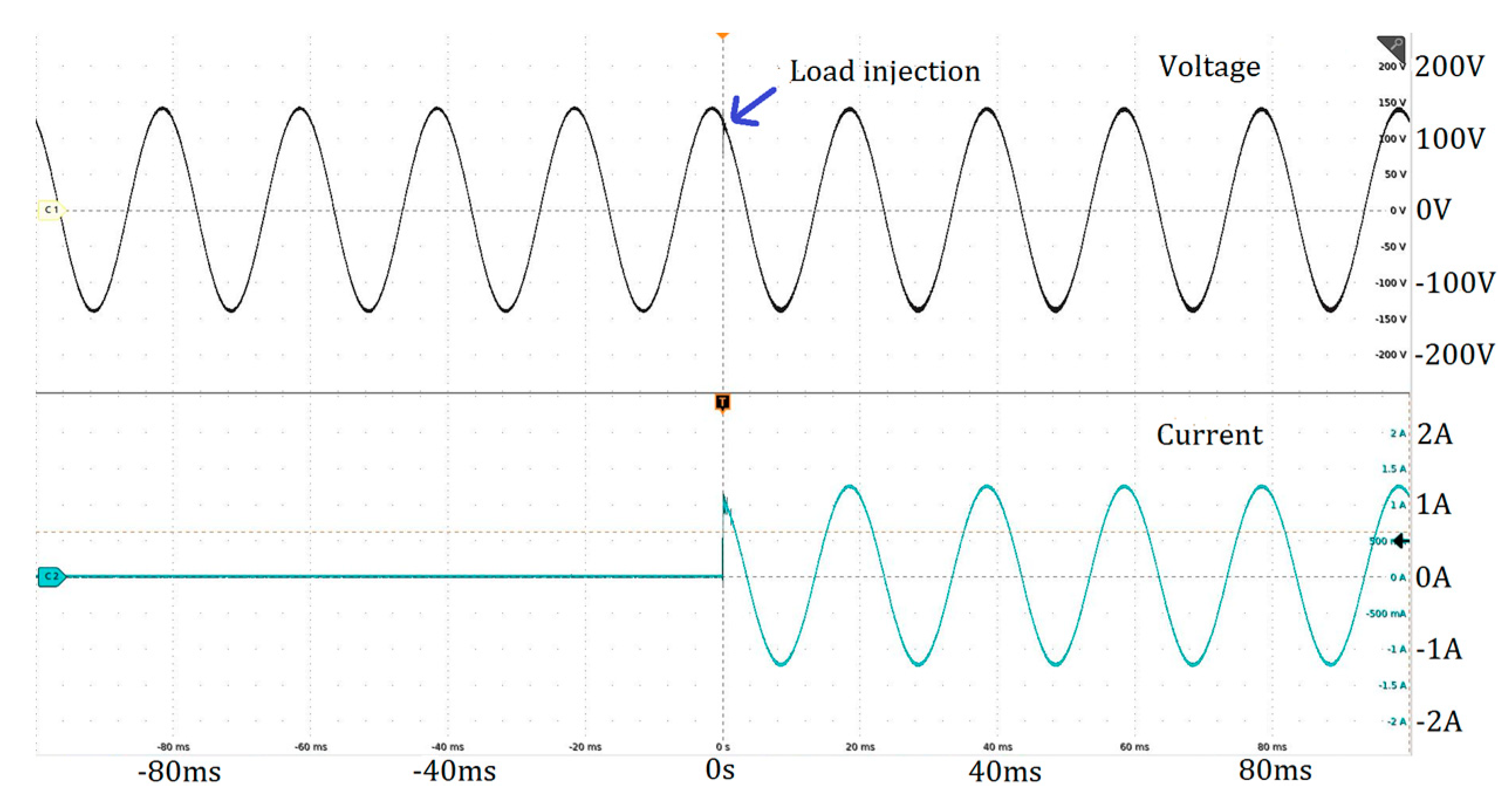
The DC sources supplied by DC generators have the voltages at 175 V. The load is a resistor with the value of . Figure 8 shows the voltage and current responses of the inverter when the load is injected. The inverter is controlled to produce an AC reference voltage, which has an effective value of 100 V, frequency of 50 Hz, and given by:
Figure 9 shows the responses of the same inverter when the reference voltage given by a DC voltage of 100 V. In both cases of the AC and DC reference voltages, the inverter yields output voltages, which are stable and match with the given reference voltages almost exactly, without transient delay. The output voltages are maintained robustly without any harmonic during the load injection.
5.2. Grid-Connected Mode
The DC voltage sources have the values of 175 V and are supplied by the same DC generators used in the stand-alone mode. The inverter is connected to a power grid with the voltage is given by:
The inverter is controlled to send a given electrical power to the grid. Figure 10 shows the voltage of the grid and the output current of the inverter when the given output power is changed from 100 W to 150 W suddenly. Figure 11 shows the responses of the same inverter when the grid voltage changes its effective value from 90 V to 100 V during sending a given power of 100 W to the grid. In all the cases, the output currents are regulated adaptively with fast and stable responses such that the inverter supplies the given powers almost exactly regardless of the sudden changes in the given power and the grid voltage. The output current of the inverter has the phase identical to that of the grid voltage.
5.3. Master Mode
The inverters are connected to a power grid with the voltage is given by:
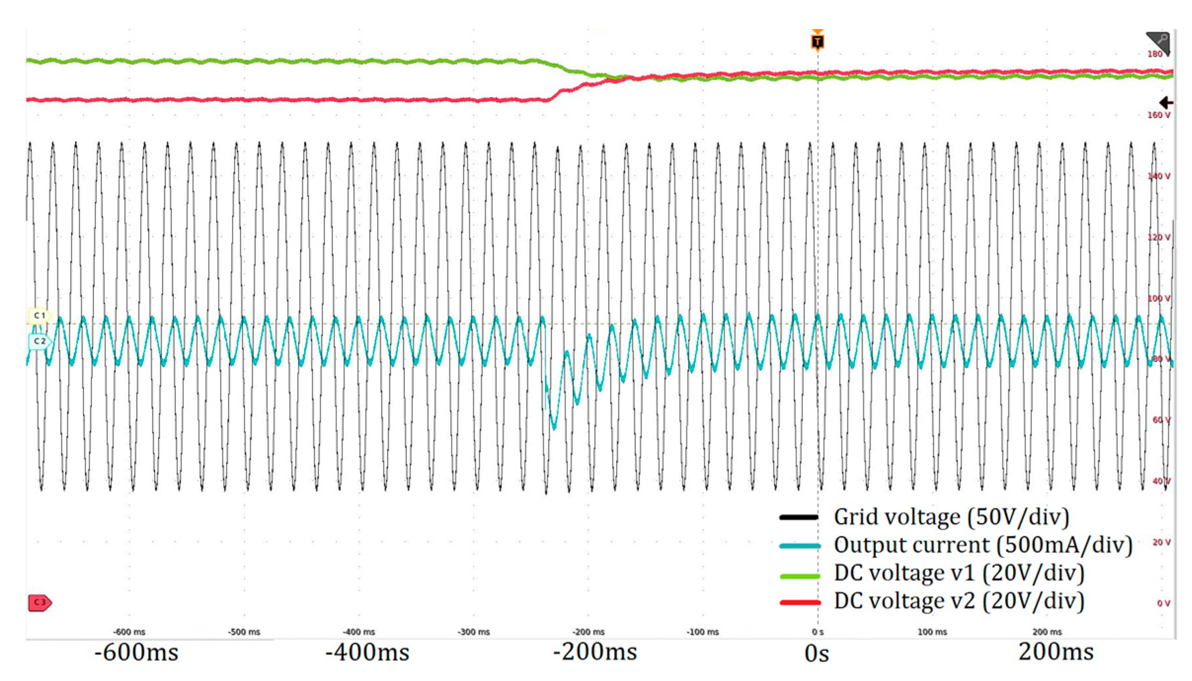
At first, the electrolytic capacitors at the DC bus of the inverter are pre-charged by the grid voltage. Each capacitor has the initial value that equals the maximum value of the grid voltage (141 V). Then, the inverter is controlled to raise the voltages and of capacitors to 175 V and maintain these voltages at that value.
Figure 12 shows the grid voltage, the output current, and the voltages of the DC bus of the inverter. In this case, the DC voltages balance at the beginning, and the amplitude of the sinusoidal term of the reference current are regulated to raise to and maintain the DC voltages at the desired value exactly.
Figure 13 shows the responses of the inverter when the DC voltages are unbalanced at the beginning. The amplitude of the sinusoidal term of the output current is regulated to raise the DC voltages while the DC term of the output current is regulated to balance the DC voltages. In all cases, the proposed control is shown to yield stable and fast responses and balances the DC voltages while maintaining them at the desired value.
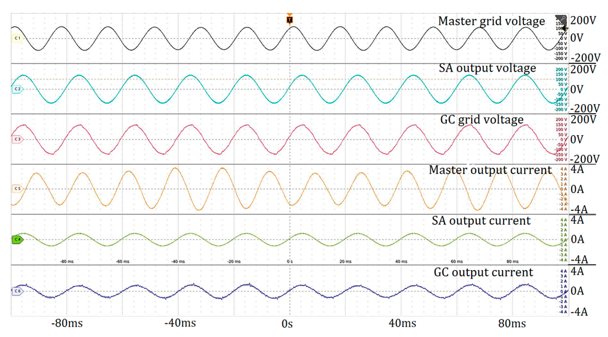
5.4. Back-to-Back System
Consider a DGR composed of the same three multi-functional inverters with a common DC bus as shown in Figure 7. In the back-to-back system, the DGR is connected to two separate power grids. The first inverter is operated in the master mode. It is connected to a power grid , which has an effective voltage value of 100 V and frequency of 60 Hz. This inverter is controlled to maintain the voltages of the common DC bus at 175 V.
The second inverter is operated in the stand-alone mode. It is controlled to supply an AC voltage to a load, which has a value of . The AV reference voltage has a frequency of 50 Hz and is given by:
The last one is operated in the grid-connected mode. It is controlled to supply a power of 100 W to a different power grid , which has an effective value of 100 V and frequency of 50 Hz.
Figure 14 shows the voltage and current responses of the master, stand-alone (SA), and grid-connected (GC) inverters respectively. The stand-alone inverter is shown to supply a voltage which matches the reference voltage almost exactly and consume a power of 100 W for the load. The grid-connected inverter transfers a power of 100 W to its grid while the master inverter receives a power of 200 W from the other grid to retain the voltages of the DC bus at 175 V. The three inverters are shown to yield stable responses and fulfill their roles almost exactly. It allows the DGR to connect to various power sources asynchronously and control the power flow smoothly.
6. Conclusions
In this paper, a digital adaptive hysteresis current control has been proposed for the multi-functional inverter in the DGR, which plays an important role in the digital grid concept. Each inverter in the DGR may be operated in the master, grid-connected or stand-alone modes, which can be specified by the software-based digital controller. The reference currents used to implement the hysteresis current control are calculated from the given reference power in the grid-connected mode, the reference voltage in the stand-alone mode, or desired voltages of the DC bus in the master mode. The controller uses high-speed sampled-data at MHz level and is implemented on the FPGA, which enable the output current to be controlled exactly with the fast dynamics. Such the FPGA-based high sampling frequency is still a new challenge in the inverter digital control area, where most of the applications are using microcomputer and DSP for the controller. This high-speed hysteresis control method with its simplicity, fast and stable response enables us to achieve the software-based multi-functional inverter. Experimental results show that the proposed control method yields stable and exact responses for the prototype of the DGR. The power packets have been transmitted between the various electrical power sources and the load in the back-to-back system asynchronously.
In our ongoing study, the digital grid system, which composes of the proposed power control in the DGR and the electricity transactions using block-chain technology, is being proving tested within a project supported by Japanese government. It is expected to produce a free-electricity market between decentralized grids and enable power grids to be adaptive to the instability due to peak-demand cutting and demand-response matching issues while accepting more and more renewable energy.
Author Contributions
T.N.-V., R.A., K.T. performed and discussed the research; T.N.-V. carried out the experiments, analyzed the data, and wrote the paper.
Funding
This research received no external funding.
Conflicts of Interest
The authors declare no conflict of interest.
References
- Asrari, A.; Wu, T.; Lotfifard, S. The Impacts of Distributed Energy Sources on Distribution Network Reconfiguration. IEEE Trans. Energy Convers. 2016, 31, 606–613. [Google Scholar] [CrossRef]
- Driesen, J.; Katiraei, F. Design for distributed energy resources. IEEE Power Energy Mag. 2008, 6, 30–40. [Google Scholar]
- Khayyer, P.; Özgüner, Ü. Decentralized Control of Large-Scale Storage-Based Renewable Energy Systems. IEEE Trans. Smart Grid 2014, 5, 1300–1307. [Google Scholar] [CrossRef]
- Marwali, M.N.; Dai, M.; Keyhani, A. Robust stability analysis of voltage and current control for distributed generation systems. IEEE Trans. Energy Convers. 2006, 21, 516–526. [Google Scholar] [CrossRef]
- Werth, A.; Kitamura, N.; Tanaka, K. Conceptual Study for Open Energy Systems: Distributed Energy Network Using Interconnected DC Nanogrids. IEEE Trans. Smart Grid 2015, 6, 1621–1630. [Google Scholar] [CrossRef]
- Abe, R.; Taoka, H.; McQuilkin, D. Digital Grid: Communicative Electrical Grids of the Future. IEEE Trans. Smart Grid 2011, 2, 399–410. [Google Scholar] [CrossRef] [Green Version]
- Buso, S.; Malesani, L.; Mattavelli, P. Comparison of current control techniques for active filter applications. IEEE Trans. Ind. Electron. 1998, 45, 722–729. [Google Scholar] [CrossRef] [Green Version]
- Irwin, J.D. Control in Power Electronics: Selected Problems, 1st ed.; Academic Press: New York, NY, USA, 2002. [Google Scholar]
- Buso, S.; Fasolo, S.; Malesani, L.; Mattavelli, P. A dead-beat adaptive hysteresis current control. IEEE Trans. Ind. Appl. 2000, 36, 1174–1180. [Google Scholar] [CrossRef]
- Malesani, L.; Tenti, P. A novel hysteresis control method for current-controlled voltage-source PWM inverters with constant modulation frequency. IEEE Trans. Ind. Appl. 1990, 26, 88–92. [Google Scholar] [CrossRef]
- Poulsen, S.; Andersen, M.A.E. Hysteresis controller with constant switching frequency. IEEE Trans. Consum. Electron. 2005, 51, 688–693. [Google Scholar] [CrossRef] [Green Version]
- Attaianese, C.; Monaco, M.D.; Tomasso, G. High Performance Digital Hysteresis Control for Single Source Cascaded Inverters. IEEE Trans. Ind. Inform. 2013, 9, 620–629. [Google Scholar] [CrossRef]
- Nguyen-Van, T.; Abe, R.; Tanaka, K. Stability of FPGA Based Emulator for Half-bridge Inverters Operated in Stand-Alone and Grid-Connected Modes. IEEE Access 2018, 6, 3603–3610. [Google Scholar] [CrossRef]
- Nguyen-Van, T.; Abe, R.; Tanaka, K. MPPT and SPPT Control for PV-Connected Inverters Using Digital Adaptive Hysteresis Current Control. Energies 2018, 11, 2075. [Google Scholar] [CrossRef]
- Hayashi, T. Power System Growth and Use of New Technologies in Japan. IEEE Power Eng. Rev. 2001, 21, 12–14. [Google Scholar] [CrossRef]
- Takagi, S. The Japanese equity market: Past and present. J. Bank. Finance 1989, 13, 537–570. [Google Scholar] [CrossRef]
- Zare, F.; Ledwich, G. A hysteresis current control for single-phase multilevel voltage source inverters: PLD implementation. IEEE Trans. Power Electron. 2002, 17, 731–738. [Google Scholar] [CrossRef] [Green Version]
- Kale, M.; Ozdemir, E. An adaptive hysteresis band current controller for shunt active power filter. Electr. Power Syst. Res. 2005, 73, 113–119. [Google Scholar] [CrossRef]
- Nguyen-Van, T.; Abe, R.; Tanaka, K. A Digital Hysteresis Current Control for Half-Bridge Inverters with Constrained Switching Frequency. Energies 2017, 10, 1610. [Google Scholar] [CrossRef]
- Vázquez, G.; Rodriguez, P.; Ordoñez, R.; Kerekes, T.; Teodorescu, R. Adaptive hysteresis band current control for transformerless single-phase PV inverters. In Proceedings of the 35th Annual Conference of IEEE Industrial Electronics, Porto, Portugal, 3–5 November 2009; pp. 173–177. [Google Scholar]
- Buso, S.; Caldognetto, T. A Nonlinear Wide-Bandwidth Digital Current Controller for DC-DC and DC-AC Converters. IEEE Trans. Ind. Electron. 2015, 62, 7687–7695. [Google Scholar] [CrossRef]
- Nguyen-Van, T.; Abe, R. An indirect hysteresis voltage digital control for half bridge inverters. In Proceedings of the IEEE 5th Global Conference on Consumer Electronics, Kyoto, Japan, 11–14 October 2016; pp. 1–4. [Google Scholar]
- Blaabjerg, F.; Teodorescu, R.; Liserre, M.; Timbus, A.V. Overview of Control and Grid Synchronization for Distributed Power Generation Systems. IEEE Trans. Ind. Electron. 2006, 53, 1398–1409. [Google Scholar] [CrossRef] [Green Version]
- Vahedi, H.; Al-Haddad, K.; Kanaan, H.Y. A new voltage balancing controller applied on 7-level PUC inverter. In Proceedings of the 40th Annual Conference of the IEEE Industrial Electronics Society (IECON), Dallas, TX, USA, 29 October–1 November 2014; pp. 5082–5087. [Google Scholar]
- Park, J.W.; Kim, J.M.; Park, S.H.; Kang, K.L.; Jung, T.U. DC voltage balancing control of half-bridge PWM inverter for linear compressor. In Proceedings of the 3rd IEEE International Symposium on Power Electronics for Distributed Generation Systems (PEDG), Aalborg, Denmark, 25–28 June 2012; pp. 598–602. [Google Scholar]
- Han, B.-M. A Half-Bridge Voltage Balancer with New Controller for Bipolar DC Distribution Systems. Energies 2016, 9, 182. [Google Scholar] [CrossRef]
- Zhang, X.; Gong, C. Dual-Buck Half-Bridge Voltage Balancer. IEEE Trans. Ind. Electron. 2013, 60, 3157–3164. [Google Scholar] [CrossRef]
- Borrega, M.; Marroyo, L.; González, R.; Balda, J.; Agorreta, J.L. Modeling and Control of a Master-Slave PV Inverter with N-Paralleled Inverters and Three-Phase Three-Limb Inductors. IEEE Trans. Power Electron. 2013, 28, 2842–2855. [Google Scholar] [CrossRef]
Figure 1.
Digital grid system with electricity trading using block-chain.

Figure 2.
Single-phase half-bridge inverter circuit.

Figure 3.
Hysteresis current control.

Figure 4.
Stand-alone inverter circuit.

Figure 5.
Grid-connected inverter circuit.
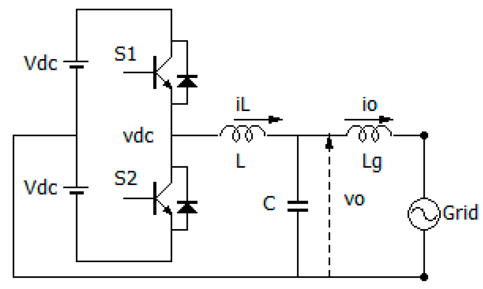
Figure 6.
Inverter circuit in master mode.

Figure 7.
The experimental inverters system. AUX: Auxiliary.

Figure 8.
Responses of the stand-alone inverter for AC reference voltage.

Figure 9.
Responses of the stand-alone inverter for DC reference voltage.
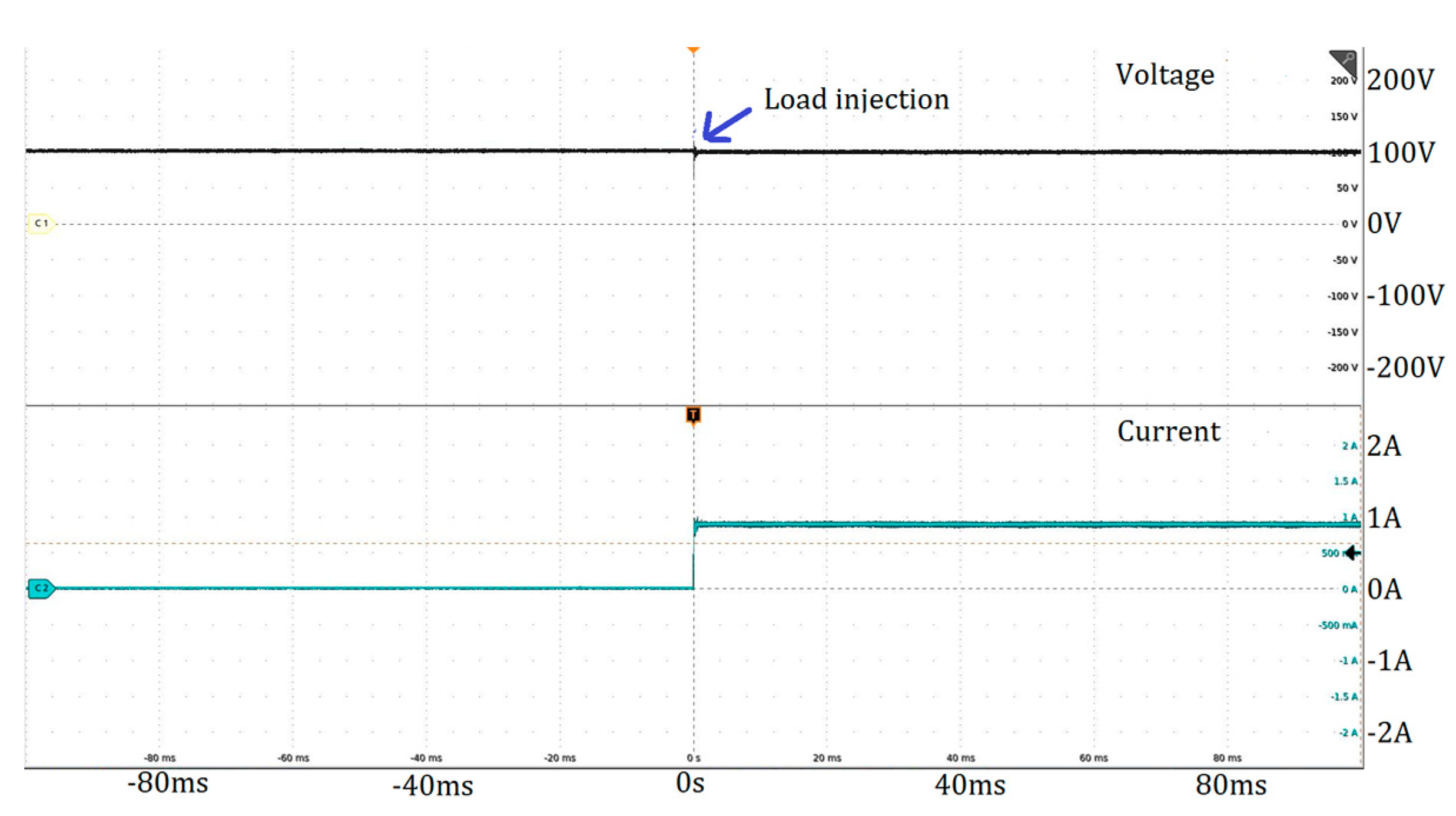
Figure 10.
Responses of the grid-connected inverter when the transferred power changes from 100 W to 150 W.
Figure 10.
Responses of the grid-connected inverter when the transferred power changes from 100 W to 150 W.
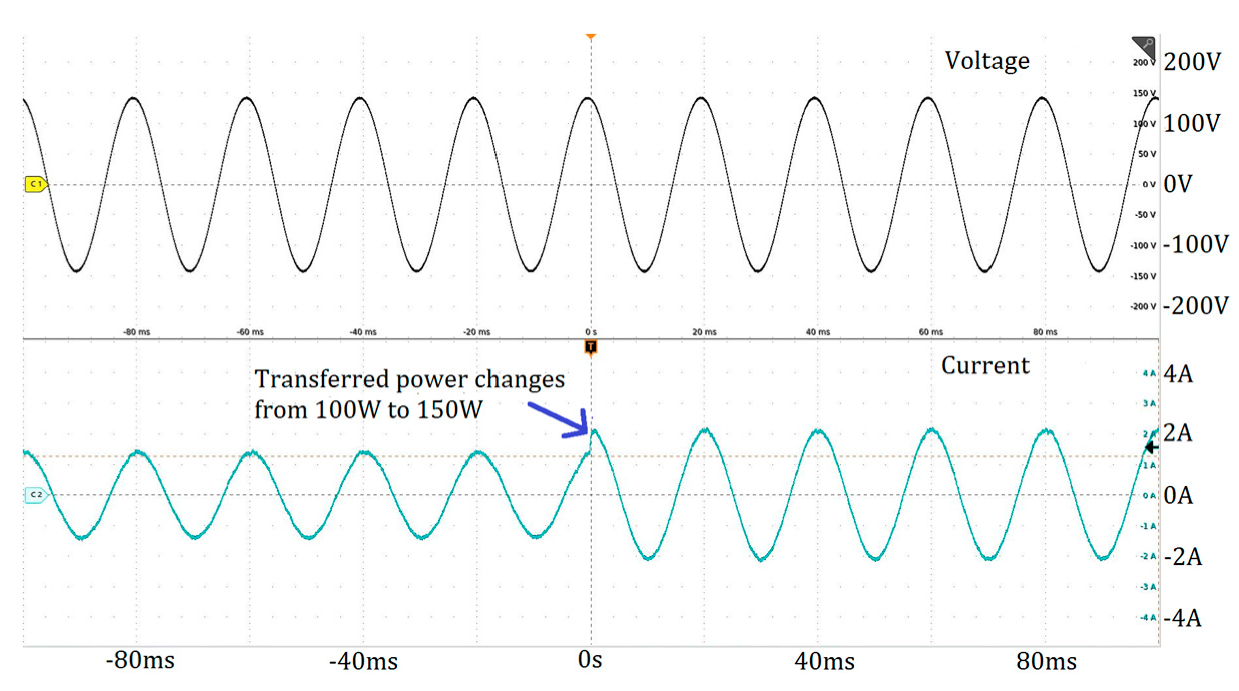
Figure 11.
Responses of the grid-connected inverter when the grid voltage changes its effective value from 90 V to 100 V.
Figure 11.
Responses of the grid-connected inverter when the grid voltage changes its effective value from 90 V to 100 V.
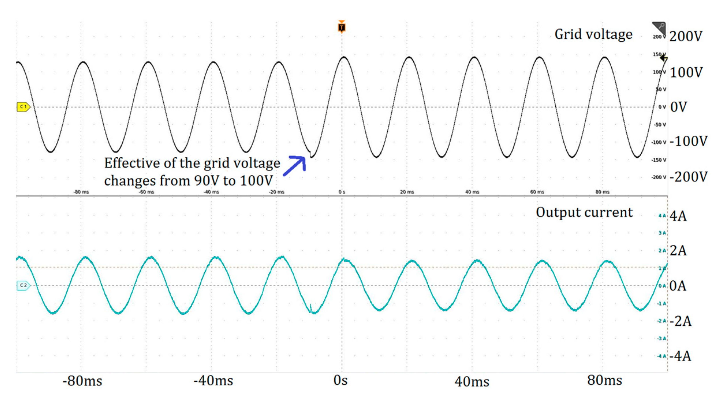
Figure 12.
Responses of the inverter in master mode when the DC voltages are maintained at desired value.
Figure 12.
Responses of the inverter in master mode when the DC voltages are maintained at desired value.
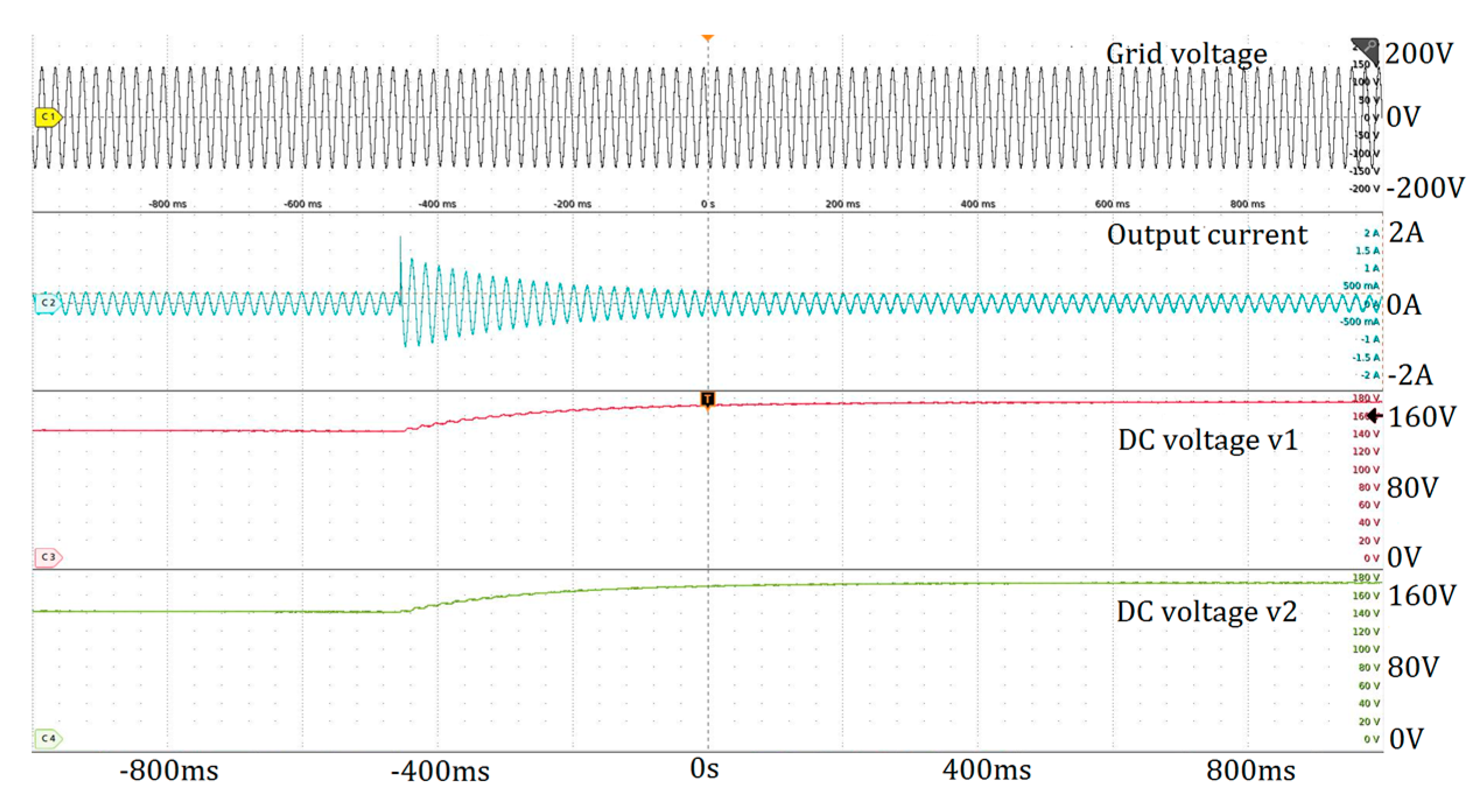
Figure 13.
Responses of the inverter in master mode when the DC voltages are imbalance.

Figure 14.
Voltage and current responses of the inverters in a back-to-back system. Abbreviations are: Stand-alone (SA), grid-connected (GC).
Figure 14.
Voltage and current responses of the inverters in a back-to-back system. Abbreviations are: Stand-alone (SA), grid-connected (GC).
© 2018 by the authors. Licensee MDPI, Basel, Switzerland. This article is an open access article distributed under the terms and conditions of the Creative Commons Attribution (CC BY) license (http://creativecommons.org/licenses/by/4.0/).
Share and Cite
MDPI and ACS Style
Nguyen-Van, T.; Abe, R.; Tanaka, K. Digital Adaptive Hysteresis Current Control for Multi-Functional Inverters. Energies 2018, 11, 2422. https://doi.org/10.3390/en11092422
AMA Style
Nguyen-Van T, Abe R, Tanaka K. Digital Adaptive Hysteresis Current Control for Multi-Functional Inverters. Energies. 2018; 11(9):2422. https://doi.org/10.3390/en11092422
Chicago/Turabian StyleNguyen-Van, Triet, Rikiya Abe, and Kenji Tanaka. 2018. "Digital Adaptive Hysteresis Current Control for Multi-Functional Inverters" Energies 11, no. 9: 2422. https://doi.org/10.3390/en11092422
Note that from the first issue of 2016, this journal uses article numbers instead of page numbers. See further details here.