Matching of Local Load with On-Site PV Production in a Grid-Connected Residential Building


1
Department of Electrical Engineering and Automation, Aalto University, 02150 Espoo, Finland
2
Electrical Engineering Department, Sharif University of Technology, Tehran 11365-11155, Iran
*
Author to whom correspondence should be addressed.
Energies 2018, 11(9), 2409; https://doi.org/10.3390/en11092409
Submission received: 23 August 2018
/
Revised: 7 September 2018
/
Accepted: 10 September 2018
/
Published: 12 September 2018
(This article belongs to the Collection Smart Grid)
Abstract
:Efficient utilization of renewable generation inside microgrids remains challenging. In most existing studies, the goal is to optimize the energy cost of microgrids by working in synergy with the main grid. This work aimed at maximizing the self-consumption of on-site photovoltaic (PV) generation using an electrical storage, as well as demand response solutions, in a building that was also capable of interacting with the main grid. Ten-minute resolution data were used to capture the temporal behavior of the weather. Extensive mathematical models were employed to estimate the demand for hot-water consumption, space cooling, and heating loads. The proposed framework is cast as mixed-integer linear programming model while minimizing the interaction with the grid. To evaluate the effectiveness of the proposed framework, it was applied to a typical Finnish household. Matching indices were used to evaluate the degree of overlap between generation and demand under different PV penetrations and storage capacities. Despite negative correlation of PV generation with Finnish seasonal consumption, a significant portion of demand can be satisfied solely with on-site PV generation during the spring and summer seasons.
1. Introduction
In recent years, a rapid growth of electricity demand was observed around the globe, which resulted in increasing energy prices and caused harmful environmental impacts such as carbon emissions. The demand increase results in more fossil-fuel consumption and faster depletion of non- renewable energy sources (non-RESs). On the other hand, the more the fossil-fuel levels decrease, the higher the price becomes. Moreover, new policies on carbon mitigation to address the concerns related to global warming enabled a contemporary shift from conventional power plants to RESs such as solar, wind, and tidal waves. However, replacing a high percentage of conventional generation with large-scale RESs adversely contributed toward the complexity of power systems by adding uncertainty that resulted in limited flexibility and increased vulnerability to overloading of networks [1]. Hence, the existing power system needs to be optimized to obtain sustainable and reliable operating conditions. An economical and promising solution to such a leapfrogging power system is taking the advantage of microgrids (MGs). An MG, as a small-scale independent power system with most of its electricity coming from local generation, mainly provided by RESs, can operate either in an islanded or interconnected mode.
The present line of research on MGs is primarily focused on minimizing the operating cost by exploiting demand response (DR) resources and employing storage facilities to cope with intermittent RESs while participating in electricity markets. Although the islanded operation of MGs may bring benefits under certain situations, in the literature, less attention is given to it. In Reference [2], to simultaneously minimize the MG operating cost and environmental impacts, as a result of importing power from the grid, a Pareto objective function was proposed. In Reference [3], the authors considered energy cost minimization in a photovoltaic (PV)-based grid-connected residential household under real-time prices. The proposed model, due to using inaccurate conventional forecasting tools, could not account for reasonable load modeling. Similarly, in Reference [4], the energy consumption of appliances through a home energy management system (HEMS) with different programming techniques was minimized for households connected to the grid. The model considered end-user discomfort levels in terms of delaying the appliance’s operation. In Reference [5], an optimal energy trading mechanism among interconnected MGs was presented wherein the DR models did not consider the end-user comfort levels, which is a crucial issue. An optimal bidding strategy for a prosumer was proposed in References [6,7] while probing the DR potential of building thermal dynamics, electric-vehicle charging, and storage facilities. The aforementioned works considered the effects of grid-connected MGs; however, the potential of islanded MGs was neglected.
One of the benefits of MGs is their intention toward matching on-site renewable generation with electricity demand. The problem of temporal matching of on-site generation and demand with one-minute time resolution was addressed in Reference [8]. The work considered PV generation and loads in a typical Finnish detached house. The revolutionary idea of net zero-energy building (ZEB) toward independent operation was studied thoroughly in References [9,10]. According to definitions in these works, a net ZEB is a grid-connected building that generates as much energy as it uses over a year. Moreover, it was highlighted that the net or nearly ZEB is capable of interacting efficiently with the distribution grid to reduce the network stresses. If a net ZEB is located in high latitude, it has high PV generation in the summer and high demand in the winter which may balance each other [11]. Such a building may supply large amounts of energy when the grid does not actually need it. Hence, there will not be a significant difference between a net ZEB and a conventional one. To utilize the full potential of green buildings, it is important to address the temporal load-matching issues in a diverse environment. In the aforementioned works, an effective framework was not considered for the utilization of on-site renewable generation in MGs or simply a green building.
This paper proposes a framework to maximize the self-utilization of on-site PV generation in a grid-connected detached house during different times of the year. This concept was naturally tailored toward a net ZEB agenda. The goal of this study was to determine the degree of being independent while relying on PV generation as much as possible. This was achieved by minimizing the power exchanges with the grid that resulted in maximizing the on-site PV consumption while exploiting flexible loads and storage devices. The load-matching index (LMI) and local-generation-matching index (LGMI) of PV were used to evaluate the degree of match or balance between PV generation and local demand. The LMI measures the fraction of the total load satisfied by the on-site generation whereas the LGMI provides information about the share of local generation that is consumed by the load. Since the weather parameters, such as solar irradiance, vary on a minute time resolution, and the calculation of the above balance metrics is time-resolution-dependent, the necessity of carrying out the study at a high time resolution is obvious. For this purpose, historical time-series data of solar irradiance and external temperature of Helsinki with ten-minute time resolution for the year 2017 were obtained from Finnish meteorological institute [12]. In the proposed model, two flexible loads, namely, electric water heater (EWH) and heating, and ventilation and air conditioning (HVAC), along with electric storage were taken into account. The main reason behind this was their major contribution to annual residential demand in Finland [13]. Also, it is worthwhile mentioning that the two loads have great flexibility mainly due to the thermal inertia of hot water and building mass [14,15,16]. The EWH is an inherent component for domestic hot-water (DHW) consumption. The temperature of hot water can be slightly altered to offer DR during hours with low PV output. For modeling the HVAC load, a two-capacity building model, which is a very efficient model for estimating the space heating or cooling demand and indoor air temperature changes with regard to outdoor temperature, was used [17]. Users usually tolerate a small deviation from the set point temperature. Hence, the ambient temperature may slightly vary inside a predefined comfort band to offer DR when required.
2. Preliminary Basics
The PV generation and load models considered in this study are briefly described in this section. These models do not constitute an original contribution of this study, but they are repeated for better understanding.
2.1. Photovoltaic Generation Model
A simple model for calculating the PV output was used in Reference [18]. The model is based on irradiance and temperature data, as well as PV characteristics, which can be found in manufacturer’s datasheet. The model is as follows:
2.2. Building Thermal Model
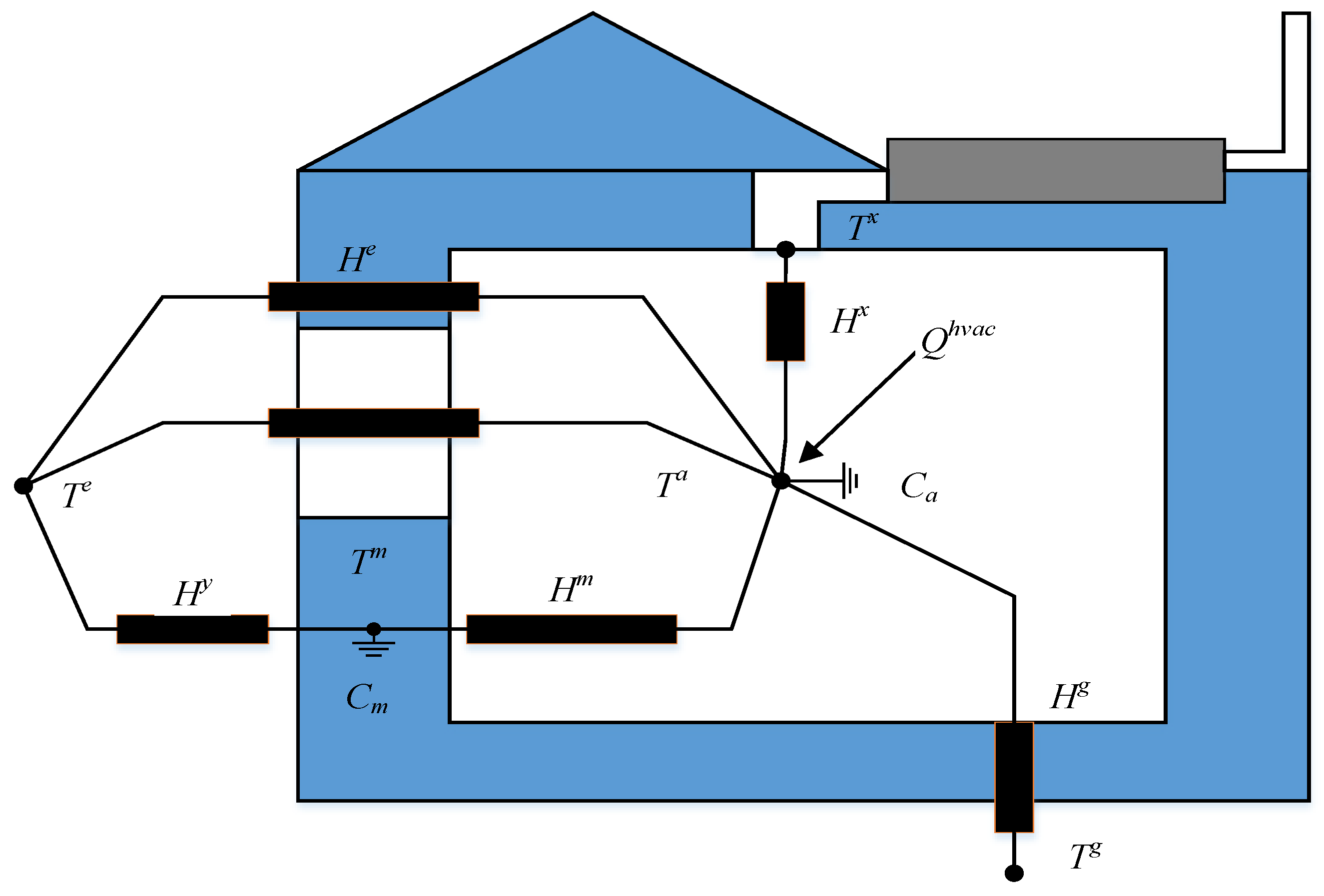
To accurately assess the space heating or cooling requirement inside a building, a two-capacity building model was utilized [17,19], which is also illustrated in Figure 1. It uses two thermal capacitances. One capacitance is assigned to the building fabric Cm, while the other capacitance Ca represents the indoor air. There are two unknown temperatures in the model, namely, building thermal mass temperature Tm and indoor air temperature Ta. Without loss of generality, it is assumed that ventilation airflows operate at constant temperature Tx. The internal heat gains from occupants and electrical appliances are assumed as negligible. The energy balance of this model is often represented by Equations (3) and (4).
2.3. Thermal Model for Electric Water Heater
This study uses the model presented in Reference [20] to represent the thermal behavior of the electric water heater. The DHW usage triggers the operation of EWH to maintain the temperature of hot water. The temperature of DHW inside the tank depends on the initial temperature of the DHW, the volume of water used in time step Δt, total volume of tank, input power, temperature of inlet cold water, and the tank thermal losses. The temperature of DHW at any instant t is a direct measure of the state of charge of the DHW tank. The temperature can be calculated as follows:
For simplicity, thermal losses are ignored in Equation (5). All parameters are given except for the temperature of hot water and the power consumption in the time slot.
3. Optimization Model
This section proposes an optimization model to maximize the consumption of on-site PV production inside a residential building tied to a grid. To do so, the objective was set to minimize the power exchange with the grid. Mathematically, the objective was represented as follows:
The objective was subject to some technical constraints and limits which ensure convenience of the user. The constraints associated with photovoltaic output, the building thermal model, and the water heater are described in the preceding section. The remaining constraints are described as follows:
Constraints (7) and (8) state that HVAC and EWH systems can be operated at any continuous power level capped by their maximum ratings. It is worthwhile to note that can take both positive and negative values depending on the external temperature. Positive values of in Equation (3) indicate that the HVAC unit is operated in heating mode, while negative values represent the cooling operation when the external temperature is higher than the HVAC set point temperature. Comfort limits for indoor ambient temperature and DHW temperature are imposed in Constraints (9) and (10), respectively. Constraints (11) and (12) ascertain that the total demand for flexible appliances, i.e., HVAC and EWH, does not change compared to business-as-usual consumption over the scheduling period, i.e., 24 h. It is worthwhile mentioning that Constraints (11) and (12) are necessary to avoid any increase in total energy consumption via activating flexibility of the appliances. The variation in state of charge of the storage is captured in Constraint (13). The charging and discharging rates of the electric storage are bounded in Constraint (14) and (15), respectively. Constraint (16) prevents the simultaneous charging and discharging of the storage. Constraint (17) restricts the state of charge (SOC) of storage within specified limits. Constraints (18) and (19) ensure that the storage is charged only from excess PV generation. In other words, the storage can be charged only if PV generation exceeds the local load. The power balance is maintained via Constraint (20). It is notable that no load or renewable generation curtailment is allowed, and that DR is not applicable to critical loads.
The resulting model is a mixed-integer nonlinear programming (MINLP) model and the existing solution approaches or commercial solvers cannot guarantee finding the global solution, although a high-quality solution might be obtained [21]. To this end, the MINLP model was reformulated into a mixed-integer linear programming (MILP) model that could be effectively embedded into an HEMS. A product of a binary variable and a continuous variable can be easily reformulated into linear expressions [22]. However, to linearize the nonlinear term related to the absolute function, two positive auxiliary variables are used. Since this absolute value is not a part of the objective function, binary variables are applied to ensure the accuracy of the linearization technique. The process is described as follows in Equations (21)–(25):
4. Case Studies and Simulation Results
A detached house with a single family in Helsinki is studied in this section. The structure of the house is assumed medium in size and it is insulated according to the minimum requirements of the Finnish Building Code C3, 2010 [23]. The typical thermal insulation levels and characteristics of the building envelope for median house structures used in this study are given in Reference [24]. The mean U-value of the building envelope is 0.47 W/m2/K. The thermodynamic two-capacity model parameters were identified using IDA, which is a simulation tool for studying the indoor climate and energy consumption of buildings [25]. The considered house was a two-floor building with a total floor area of 200 m2, i.e., 100 m2 per floor, and the parameter values of the two-capacity model for this house are listed in Table 1. Please note that the given parameters are applicable to Finnish detached houses only.
The house was equipped with PV modules, an HVAC unit, EWH and some critical load. The house was also equipped with an HEMS to prioritize the consumption of the PV modules. It was connected to a distribution grid through an interconnection with a high capacity, enabling electricity exchanges at a flat tariff. It was assumed that 10 PV modules of 500 Wp each were installed on the roof. We considered Sunpreme-made [26] PV modules with specifications detailed in Table 2.
The rating of the HVAC unit was 6 kW with 100% efficiency. The ambient temperature preference was set to 21 °C and the ground node temperature Tg was assumed constant at 10 °C. The EWH was rated 2 kW with the total volume of DHW tank as 200 L. Hot-water temperature priority was 60 °C. It was assumed that temperature of inlet cold water for EWH operation was 10 °C. Furthermore, without loss of generality, it was assumed that the daily DHW consumption profile of a household remained the same throughout a year [27]. The DHW profile is depicted in Figure 2 [28]. According to statistics provided in Reference [27], the total daily consumption considered here is well suitable for a dwelling occupied by 3–4 persons in Finland. Building occupancy was rendered continuous over the study period. Initial ambient and DHW temperatures were set to 21 °C and 60 °C, respectively. It was assumed that the weather parameters for the following day could be forecasted without significant uncertainties. The critical load used in this study were the energy consumption data of a typical residential consumer in Helsinki relying on a district heating facility for space heating, cooling, and hot-water consumption. The profile of such a consumer, thus, contains only the critical load.
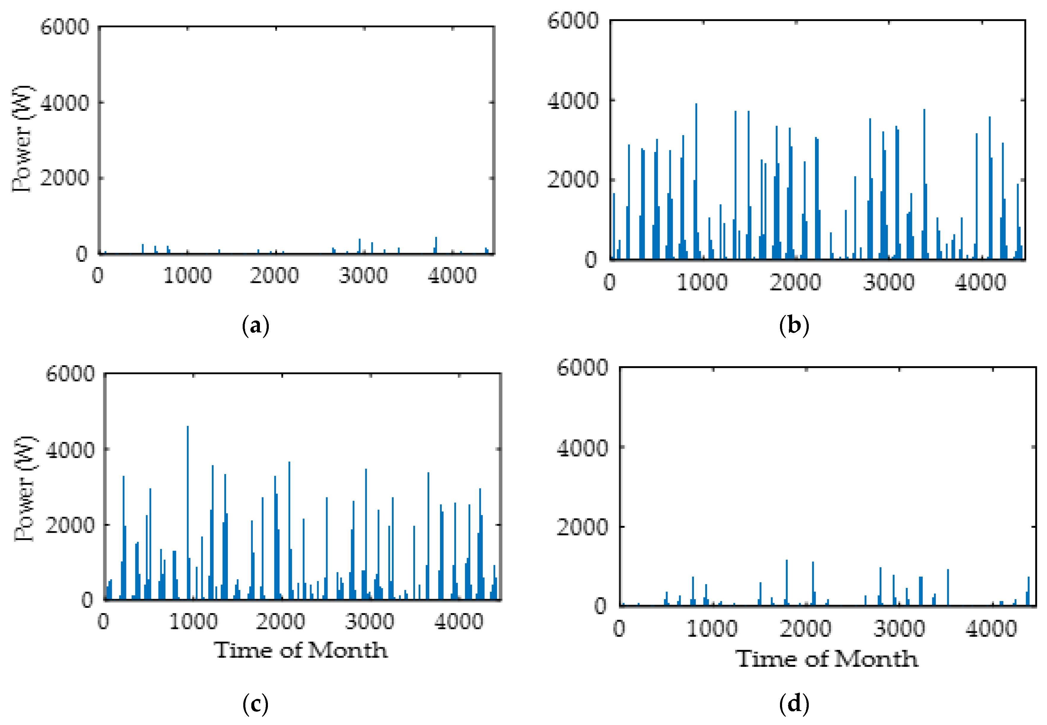
The months of January, May, July, and October were selected to represent winter, spring, summer, and autumn seasons, respectively, and the simulation was performed for each day of the representative months separately and serially. In general, LMI and LGMI indices may experience significant day-to-day variations within a month. Therefore, the indices computed in this study were the average of daily indices over the month. Considering ten-minute resolution, there were 144 time slots per day. Figure 3 depicts the PV generation in different seasons obtained using Equations (1) and (2). According to the PV generation profiles, the capacity factors of PV for the winter, spring, summer, and autumn seasons were 0.438%, 17.14%, 14.82%, and 1.824%, respectively.
Simulations were performed on Matlab software while the optimization problem was solved in GAMS using the CPLEX solver. The simulations were performed for the following four case studies:
- Case I: In this case, the model was solved for the base case considering no storage and DR. This case serves as a comparison benchmark for other cases.
- Case II: In this case, only the storage option was considered as available flexibility to minimize the power exchanges with the grid.
- Case III: Here, only DR was employed instead of the storage option.
- Case IV: The complete proposed model including both storage and DR options was simulated in this case.
In addition to the above case studies, sensitivity analyses were performed to investigate the impact of increasing PV generation and storage capacities on the matching indices.
4.1. Case I: The Base Case without Storage and DR
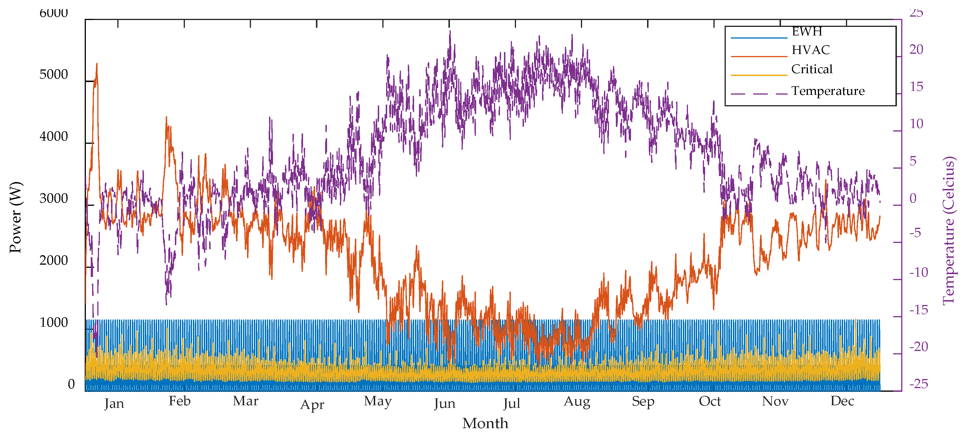
The proposed model was simulated for all seasons under strict comfort requirements, i.e., ambient temperature and DHW temperature were maintained at 21 °C and 60 °C, respectively, for all 4464 time slots. The disaggregated annual loads calculated using Equations (3)ߝ(5), along with the temperature profile, are illustrated in Figure 4. It can be seen that the HVAC loads heavily contributed to the total residential load during all seasons. The ambient temperature needed to be obliged at all times. In contrast, EWH loads depended on the DHW usage which was dominant in specific hours during the daytime only. The negative correlation of PV output with Finnish seasonal consumption is evident from Figure 3 and Figure 4.
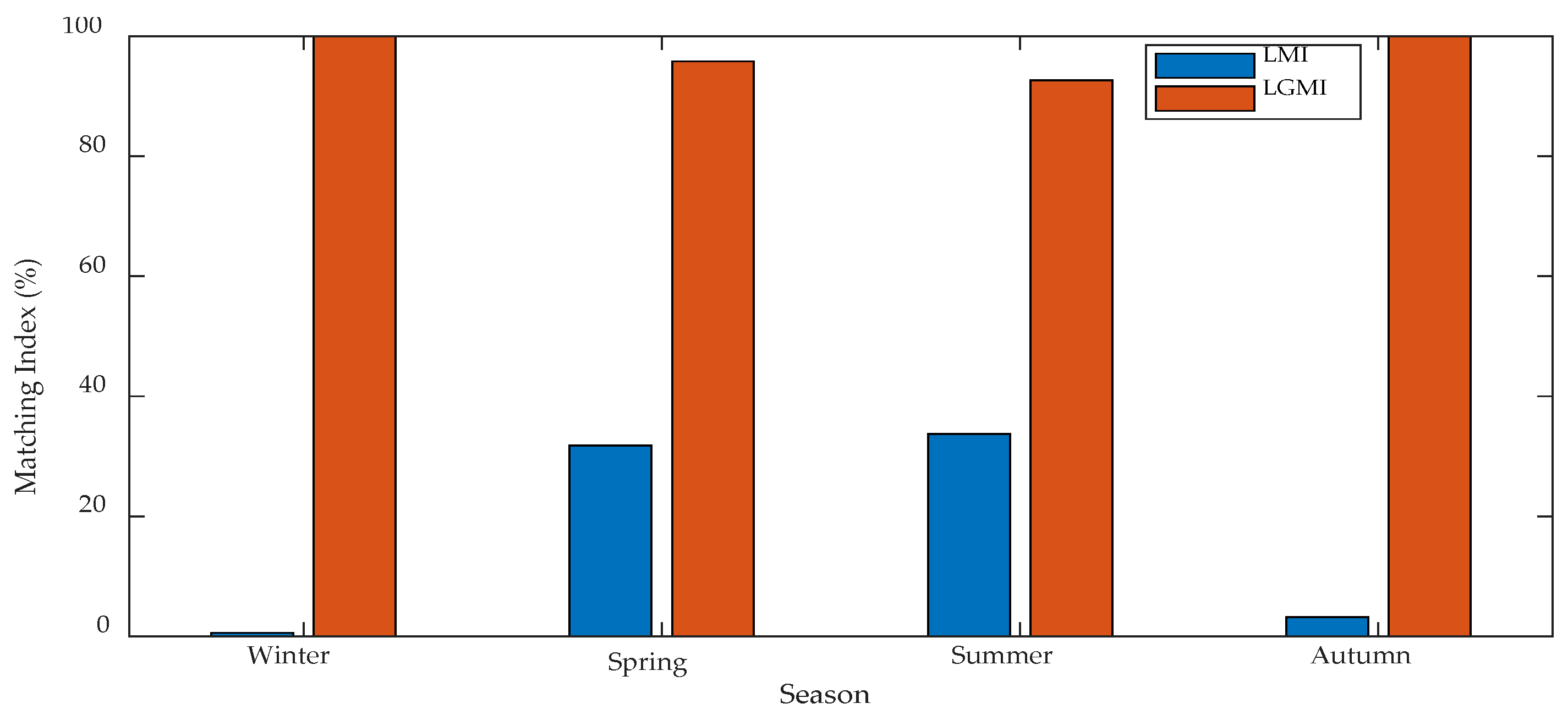
LMI and LGMI were calculated for the simulated loads and PV generation using Equations (26) and (27), respectively, and the results are displayed in Figure 5. For this case, due to low PV generation in the winter and autumn, the resulting LMI was very low but LGMI values indicated that the entire PV generation was consumed by the load. Due to the diurnal cycle of PV, a full load could not be satisfied with PV even in the summer and spring seasons. Moreover, some PV generation was exported to the grid in these seasons. The results indicate the need of demand-side flexibility and/or a storage system in order to better utilize the PV generation.
4.2. Case II: Matching of Demand and PV Generation Using Storage
In this case, an electric storage of 10 kWh capacity was integrated into the HEMS. The charging and discharging efficiencies were assumed to be 90% each. It was assumed that the initial SOC was 25% of the rated capacity at the beginning of the simulation and the resulting SOC at the end of each day in a month was made available for the next day in each simulation. The storage stored the excess amount of PV production during the day time so that it could be utilized later when PV production was negligible or zero. The storage could not take part in power exchanges with the grid. The remaining simulation parameters remained the same as in Case I. To showcase the effectiveness of the model, the operation of two consecutive days of spring are demonstrated in Figure 6. Undoubtedly, the storage operation was more demanding due to high PV generation in this season. The matching indices calculated in this case are illustrated in Figure 7. The improvement in the indices was substantial in the case of spring and summer seasons. Indices for summer and spring were improved due to high PV productions in these periods. The improvements in LMI were 18.05% and 33.51% for the spring and summer seasons, respectively. However, there was also a slight improvement in LGMI for these two seasons. The LMI improvements in the other seasons were not significant due to very low PV production. It is worthwhile pointing out that the proposed objective function targeted both matching indices since both of them improved in comparison to the first case.
4.3. Case III: Matching of Demand and PV Generation Using DR
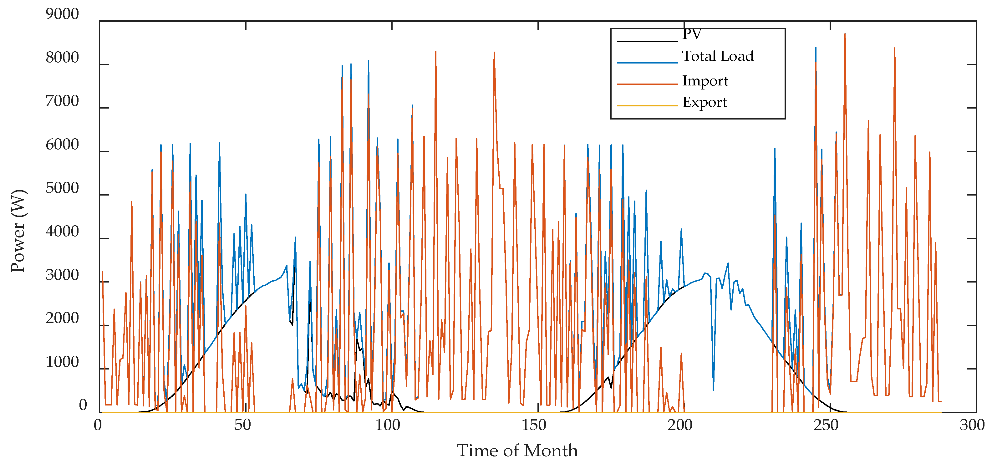
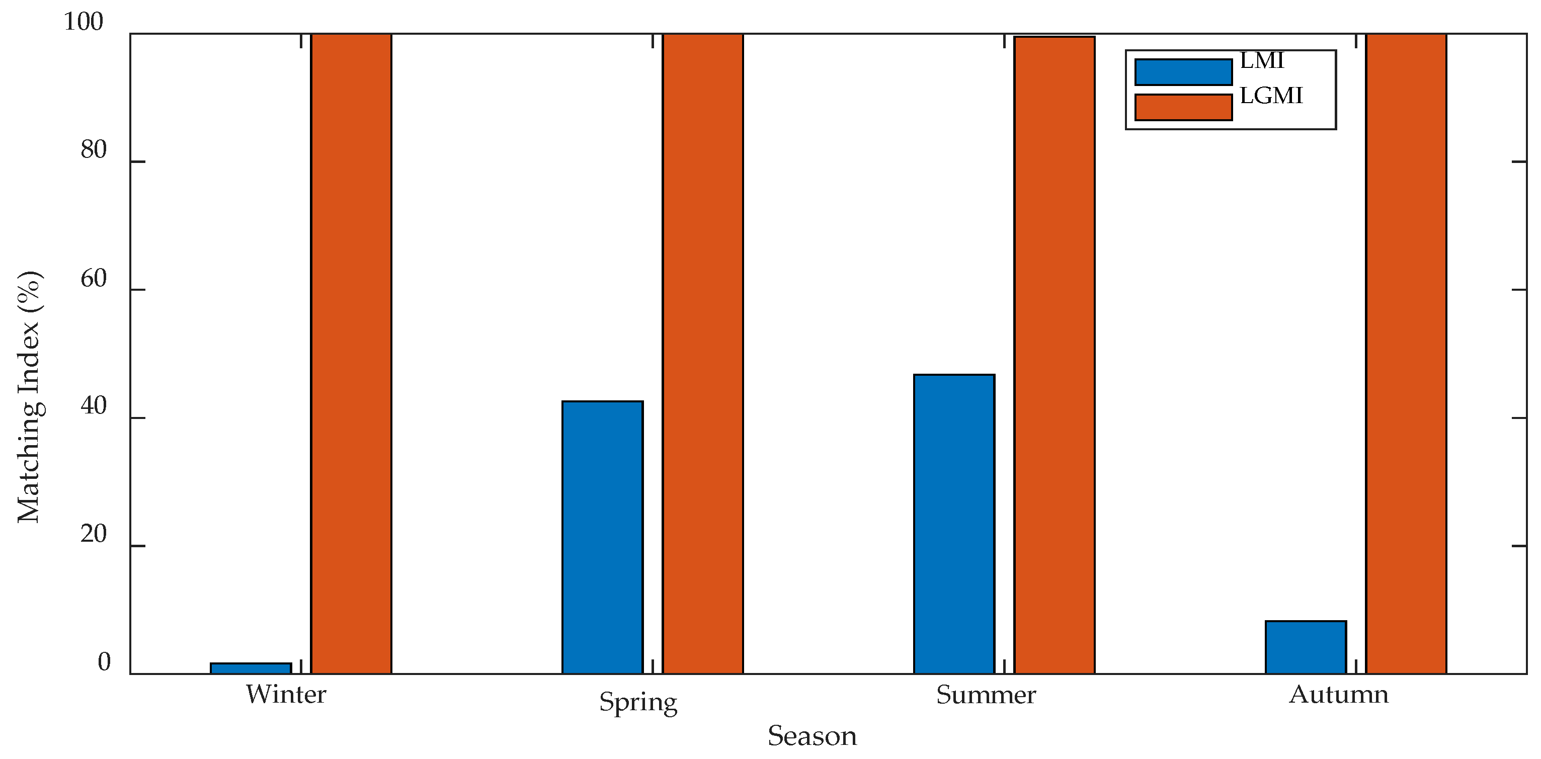
Here, it was assumed that the temperature of DHW could range between 55 °C and 65 °C, which is in accordance with the Finnish building code. The ambient temperature of the house could hover between 20.5 °C and 21.5 °C, i.e., a temperature dead band of 1 °C. It must be noted that such a minor variation from the HVAC set point does not result in discomfort as long as the total HVAC demand remains constant. There is no storage device in this case. Figure 8 illustrates that the DR provided a high-ramping capability of matching the consumption with PV production, thanks to building thermal inertia. This is due to the high portion of HVAC loads in the total residential demand (see Figure 4). It can be seen that total load was perfectly matched with PV production for some time slots. At times when there was no PV generation, the imported power was equal to the total load, which is visible in Figure 8. The calculated LMI and LGMI indices are depicted in Figure 9. The values imply that the DR option is more feasible compared to the 10 kWh storage. Compared to the first case, the improvements in LMI were 34% and 38.58% for spring and summer seasons, respectively. Moreover, this DR framework also improved the LMI for winter and autumn seasons to a reasonable extent.
4.4. Case IV: Matching of Demand and PV Generation Using Both Storage and DR
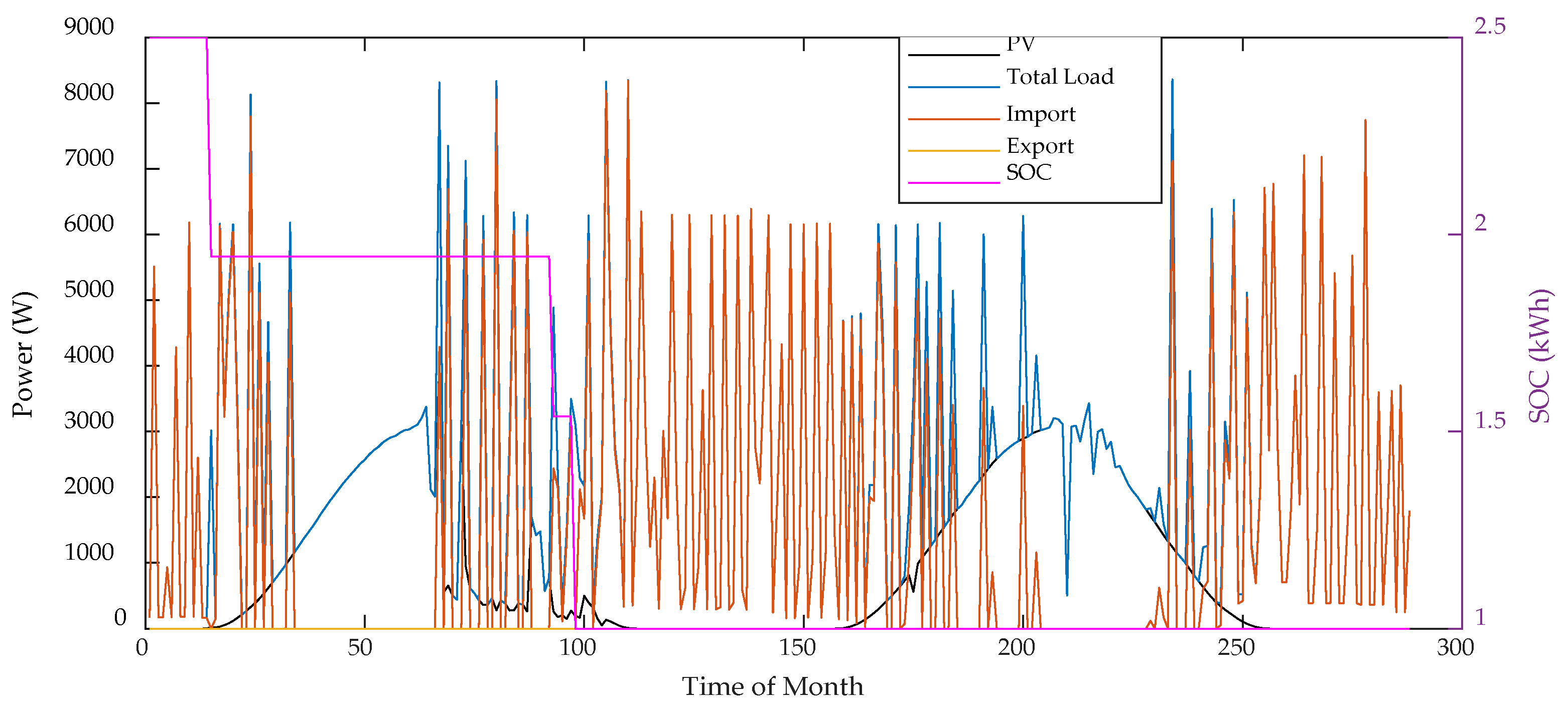
We utilized both the storage and DR options in this case. The parameters of storage and DR load remained the same as in Cases II and III, respectively. According to the obtained results, the DR option in coordination with the storage facility promised even better matching capability. The power balance for the same two days of spring is illustrated in Figure 10. It can be seen that the storage operation was limited due to DR. Instead, the building itself acted as small storage buffer. The building stored the heat energy in its thermal masses. The ramping capability of HVAC loads was much higher compared to the storage, which has limited charging and discharging power. The calculated LMI and LGMI indices are depicted in Figure 11. As can be seen, the LMI indices for all seasons were improved without compromising on LGMI. LMI indices of 46.43% and 51.83% were achieved for spring and summer seasons, respectively. Compared to the base case, there were 46.05% and 53.7% improvements in LMI for spring and summer seasons, respectively. The proposed model resulted in the full self-utilization of PV production in all seasons, as clearly seen in the LGMI values.
The dynamics of the matching indices obtained for different cases and seasons are summarized in Table 3. It can be inferred from the trend that summer and spring are the seasons in which matching can be improved significantly in Finland. High values of these indices imply that there is less power exchange with the grid. Ideally, if LMI is 100%, then load is perfectly matched with PV generation and the imported power is zero. Similarly, if LGMI is 100%, then power exported to the grid is zero.
4.5. Sensitivity Analyses
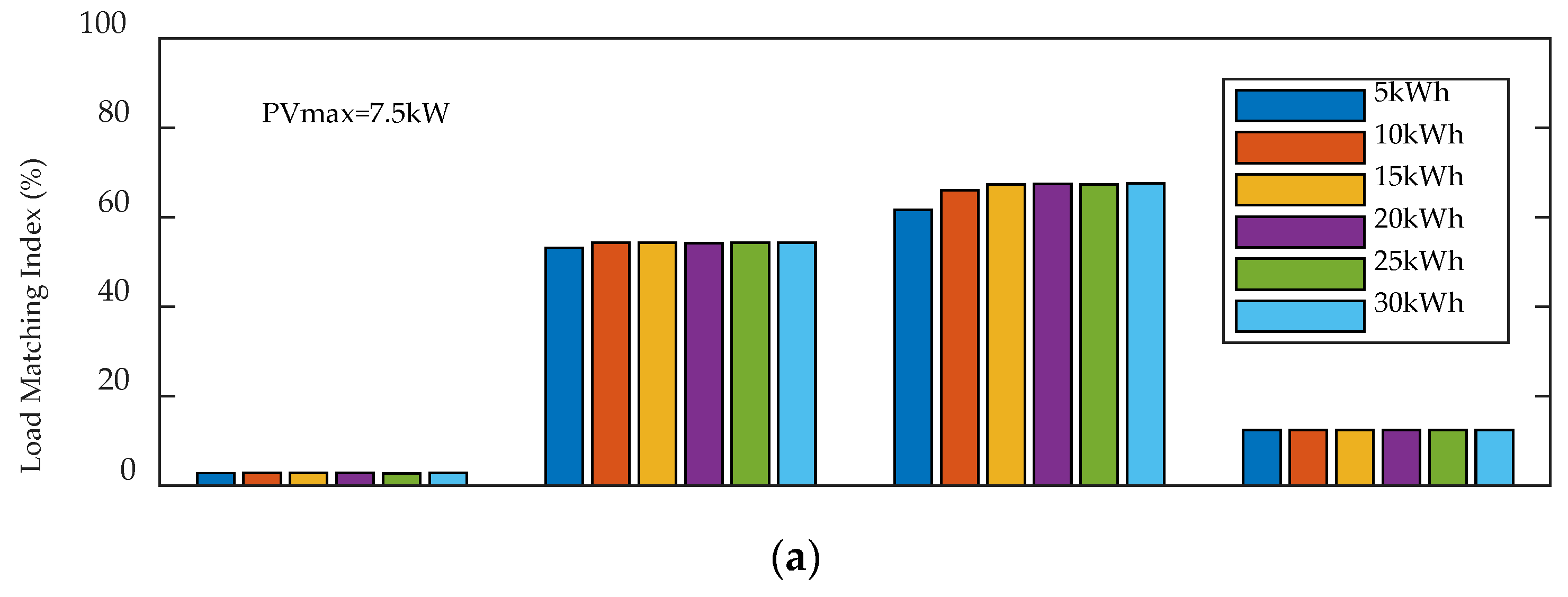
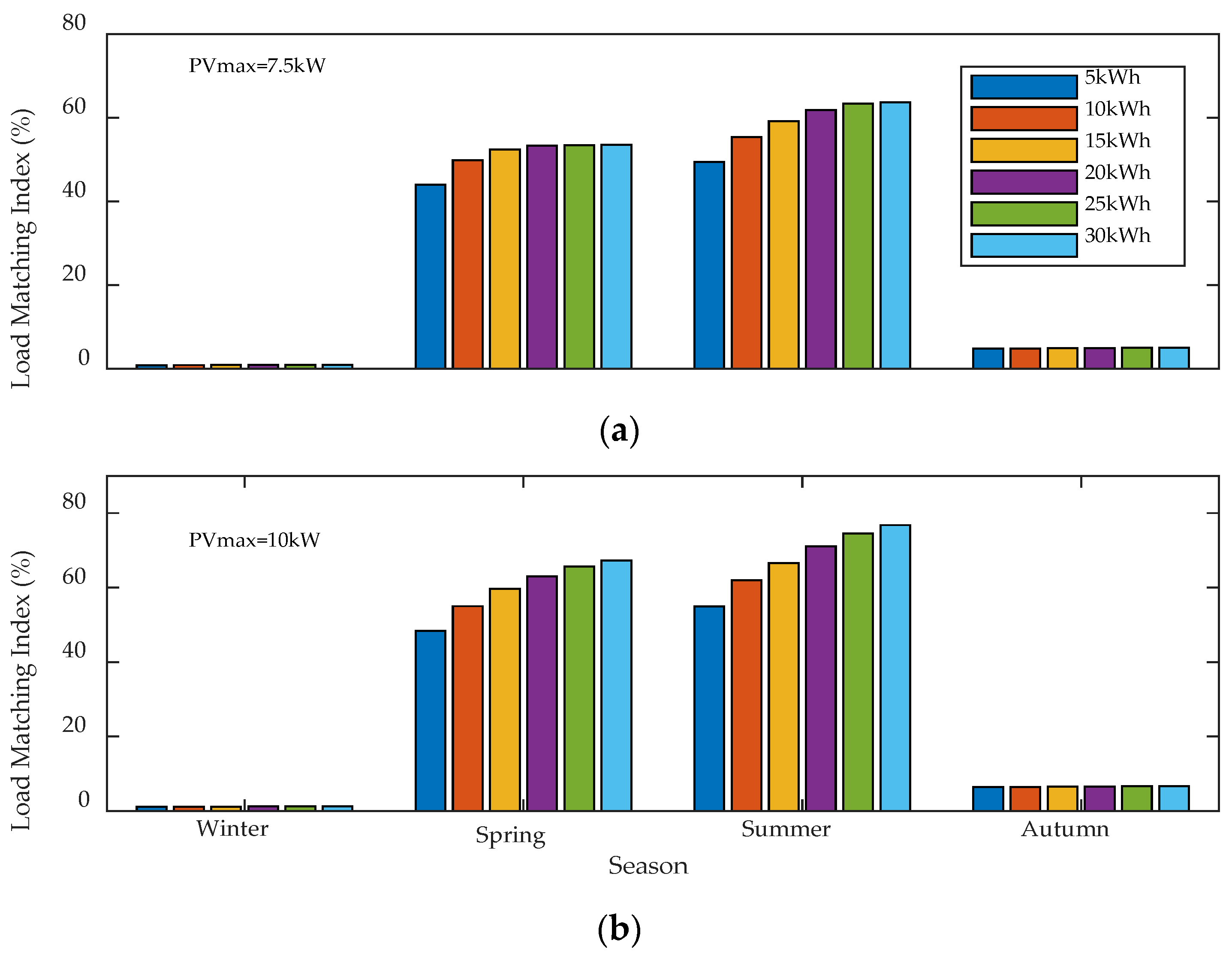
In this sub-section, sensitivity analyses were performed to study the influence of increasing PV generation and storage capacities on the LMI for Cases II and IV. In Figure 12, the effects of increasing the storage size from 5 kWh to 30 kWh, with 5 kWh steps, on the LMI for two different PV ratings of 7.5 kW and 10 kW are shown. For both PV capacities, in the spring and summer seasons, the LMI generally improved with increasing the storage capacity. Moreover, it can be seen that, in the spring season for the PVmax equal to 7.5 kW, there was no improvement in the LMI for higher storage capacities, which implies that the PV production was not enough to efficiently utilize the full storage capacity. However, there is a very small improvement for winter and autumn seasons. This might have been due to low and random PV generation in the winter and autumn that did not follow the exact diurnal pattern, which is also evident from Figure 3. The storage size did not have any substantial effect on these seasons. An LMI of 76.78% could be achieved in summer with a 10 kW peak of PV and a storage capacity of 30 kWh. As can be seen in Figure 12b for the spring and summer, unlike Figure 12a, increasing the storage capacity affected the LMI together with a higher PV capacity.
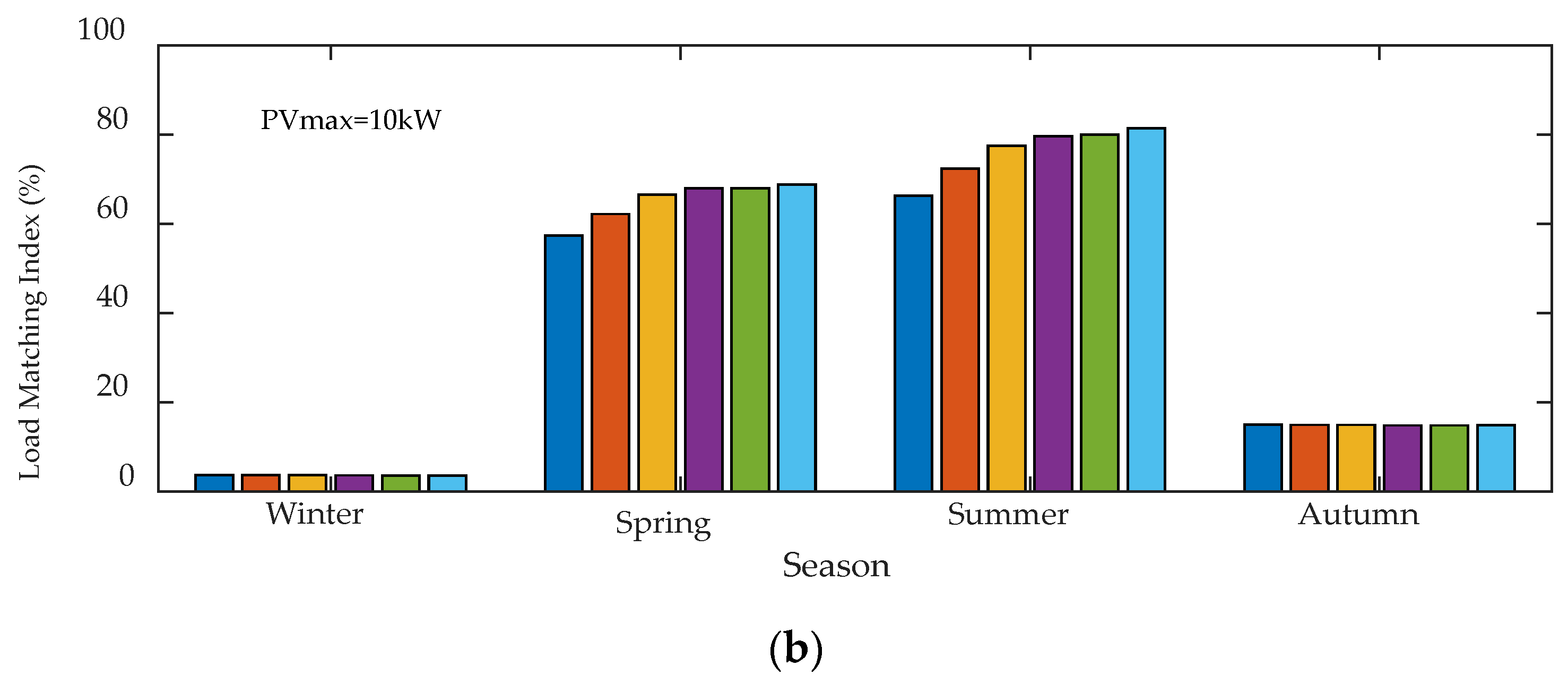
Figure 13 illustrates the dynamics of LMI in the presence of both the storage and DR options, i.e., Case IV. Compared to Figure 12, this coordination with the DR resulted in LMI improvements for all seasons; however, it can be seen that less storage capacity was necessary to reach more or less the same LMI. For example, in Figure 12a for the spring season, the maximum LMI was obtained after investing in a storage device with 20 kWh capacity, while, in Figure 13a, roughly the same LMI was obtained by investing in only 5 kWh storage. Here, the combined benefits of storage and DR were the main reason for such an outcome. For lower storage sizes, the coordination results in better matching than using just the storage devices. The major reason is the limited operation of storage in the presence of building thermal dynamics. The efficiency of storage also plays a prominent role at higher capacities. However, an LMI of 81.37% was achieved for the summer with PVmax = 10 kW and a storage capacity of 30 kWh.
5. Conclusions
This paper studied the potential of supplying local load with on-site PV generation. The proposed model uses storage and DR options to maximize the self-utilization of PV generation in a grid-connected detached house. LMI and LGMI were used to evaluate the degree of match. The results indicate that there is a high seasonal variation between the match of load and local generation in Finland. In Finnish conditions, a small-size storage system coordinated with DR was proven to be a very promising solution to address the load-matching issue. This study utilized electric storage, while domestic-storage space heaters are also another option to be considered. However, both storage systems serve a similar purpose with respect to the load-matching issue. It was also found that LMI and LGMI could be significantly improved for spring and summer seasons, as local PV generation is higher in these seasons. However, such improvements require a huge investment in PV and storage technologies for independent operation of the building.
Author Contributions
A.A.B. performed the simulations and prepared the original research draft; M.P.K. and A.S. provided the support in formulating the optimization problem and its implementation in GAMS; M.L. proposed the main idea and supervised the work.
Funding
This research was funded by Aalto University as part of the Finnish Solar Revolution (FSR) project organized by “Business Finland”.
Conflicts of Interest
The authors declare no conflict of interest.
Nomenclature
| Indices and sets | |
| t, T | Index and set of time slot |
| Parameters | |
| Specific heat capacity of water (J/kg/K) | |
| Indoor air heat capacity (J/°C) | |
| Building fabric capacity (J/°C) | |
| HVAC daily demand for consumption as usual (W·h) | |
| EWH daily demand for consumption as usual (W·h) | |
| Solar constant, i.e., 1000 W/m2 | |
| Heat conductance (W/°C) between external air and indoor air node points | |
| Heat conductance (W/°C) between indoor air and ground node points | |
| Heat conductance (W/°C) between indoor air and building mass node points | |
| Heat conductance (W/°C) between external air and building mass node points | |
| Heat conductance (W/°C) between HVAC air and indoor air node points | |
| Short-circuit current of a PV cell (A) | |
| M | A big number |
| NOCT | Normal operating cell temperature of PV module (K) |
| Rated maximum yield of the PV system (W) | |
| Rated maximum power of EWH (W) | |
| Critical load at time t (W) | |
| Rated maximum power of HVAC unit (W) | |
| S | Insolation level (mW/cm2) |
| Maximum and minimum limits for SOC of electric storage (Wh) | |
| Maximum and minimum limits for ambient temperature (°C) | |
| External temperature at time t (°C) | |
| Temperature of the ventilation air (°C) | |
| Temperature of inlet cold water in the hot water tank (°C) | |
| Ground node temperature (°C) | |
| Reference cell temperature of PV module (°C) | |
| Maximum and minimum limits for DHW temperature (°C) | |
| Volume of hot water tank of household (L) | |
| Volume of hot water used at time t (L) | |
| Charging/discharging efficiency of electric storage | |
| Variables | |
| Charging and discharging decisions of electric storage at time t | |
| Binary decisions associated with auxiliary variables | |
| electric storage balance at time t (W) | |
| Total generation from the RES at time t (W) | |
| Irradiance at time t (W) | |
| Total load at time t (W) | |
| EWH power consumption at time t (W) | |
| Charging and discharging power of electric storage at time t (W) | |
| Power flow from the building to electrical grid (W) | |
| Power flow from the electrical grid into the building (W) | |
| PV production at time t (W) | |
| HVAC power consumption at time t (W) | |
| Positive auxiliary variables for HVAC power consumption at time t (W) | |
| SOC of electric storage at time t (W·h) | |
| PV cell operating temperature at time t (K) | |
| Ambient temperature at time t (°C) | |
| DHW temperature at time t (°C) | |
| Building mass temperature at time t (°C) | |
References
- Guo, Y.; Pan, M.; Fang, Y. Optimal Power Management of Residential Customers in the Smart Grid. IEEE Trans. Parallel Distrib. Syst. 2012, 23, 1593–1606. [Google Scholar] [CrossRef]
- Di Somma, M.; Graditi, G.; Heydarian-Forushani, E.; Shafie-khah, M.; Siano, P. Stochastic optimal scheduling of distributed energy resources with renewables considering economic and environmental aspects. Renew. Energy 2018, 116, 272–287. [Google Scholar] [CrossRef]
- Yoo, J.; Park, B.; An, K.; Al-Ammar, E.A.; Khan, Y.; Hur, K.; Kim, J.H. Look-ahead energy management of a grid-connected residential pv system with energy storage under time-based rate programs. Energies 2012, 5, 1116–1134. [Google Scholar] [CrossRef]
- Iqbal, Z.; Javaid, N.; Iqbal, S.; Aslam, S.; Khan, Z.; Abdul, W.; Almogren, A.; Alamri, A. A Domestic Microgrid with Optimized Home Energy Management System. Energies 2018, 11, 1002. [Google Scholar] [CrossRef]
- Nguyen, D.T.; Le, L.B. Optimal energy management for cooperative microgrids with renewable energy resources. In Proceedings of the IEEE International Conference on Smart Grid Communications (SmartGridComm), Vancouver, BC, Canada, 21–24 October 2013; pp. 678–683. [Google Scholar]
- Nguyen, D.T.; Le, L.B. Optimal bidding strategy for microgrids considering renewable energy and building thermal dynamics. IEEE Trans. Smart Grid 2014, 5, 1608–1620. [Google Scholar] [CrossRef]
- Nguyen, D.T.; Le, L.B. Joint Optimization of Electric Vehicle and Home Energy Scheduling Considering User Comfort Preference. IEEE Trans. Smart Grid 2014, 5, 188–199. [Google Scholar] [CrossRef]
- Degefa, M.Z.; Lehtonen, M.; McCulloch, M.; Nixon, K. Real-time matching of local generation and demand: The use of high resolution load modeling. In Proceedings of the IEEE PES Innovative Smart Grid Technologies Conference Europe (ISGT-Europe), Ljubljana, Slovenia, 9–12 October 2016; pp. 1–6. [Google Scholar]
- Sartori, I.; Napolitano, A.; Voss, K. Net zero energy buildings: A consistent definition framework. Energy Build. 2012, 48, 220–232. [Google Scholar] [CrossRef] [Green Version]
- Salom, J.; Marszal, A.J.; Widén, J.; Candanedo, J.; Lindberg, K.B. Analysis of load match and grid interaction indicators in net zero energy buildings with simulated and monitored data. Appl. Energy 2014, 136, 119–131. [Google Scholar] [CrossRef]
- Salom, J.; Widén, J.; Candanedo, J.; deM Sartori, I.A.; Voss, K.; Marszal, A. Understanding Net Zero Energy Buildings: Evaluation of Load Matching and Grid Interaction Indicators. Proc. Build. Simul. 2011, 6, 2514–2521. [Google Scholar]
- Finnish Meteorological Institute. 2018. Available online: http://en.ilmatieteenlaitos.fi/ (accessed on 1 May 2018).
- Statistics Finland. 2018. Available online: www.stat.fi/til/index_en.html (accessed on 1 May 2018).
- Safdarian, A. Coordinated Management of Residential Loads in Large-Scale Systems; Springer International Publishing: Cham, Switzerland, 2018; pp. 151–171. [Google Scholar]
- Ali, M.; Safdarian, A.; Lehtonen, M. Risk-constrained framework for residential storage space heating load management. Electr. Power Syst. Res. 2015, 119, 432–438. [Google Scholar] [CrossRef]
- Safdarian, A.; Ali, M.; Fotuhi-Firuzabad, M.; Lehtonen, M. Domestic ewh and hvac management in smart grids: Potential benefits and realization. Electr. Power Syst. Res. 2016, 134, 38–46. [Google Scholar] [CrossRef]
- Ali, M.; Degefa, M.Z.; Humayun, M.; Safdarian, A.; Lehtonen, M. Increased utilization of wind generation by coordinating the demand response and real-time thermal rating. IEEE Trans. Power Syst. 2016, 31, 3737–3746. [Google Scholar] [CrossRef]
- Jones, A.D.; Underwood, C.P. A modelling method for building-integrated photovoltaic power supply. Build. Serv. Eng. Res. Technol. 2002, 23, 167–177. [Google Scholar] [CrossRef]
- Ali, M.; Ekström, J.; Lehtonen, M. Sizing Hydrogen Energy Storage in Consideration of Demand Response in Highly Renewable Generation Power Systems. Energies 2018, 11, 1113. [Google Scholar] [CrossRef]
- Shao, S.; Pipattanasomporn, M.; Rahman, S. Development of physical-based demand response-enabled residential load models. IEEE Trans. Power Syst. 2013, 28, 607–614. [Google Scholar] [CrossRef]
- Pourakbari-Kasmaei, M.; Sanches Mantovani, J.R. Logically constrained optimal power flow: Solver-based mixed-integer nonlinear programming model. Int. J. Electr. Power Energy Syst. 2018, 97, 240–249. [Google Scholar] [CrossRef]
- Melgar Dominguez, O.D.; Pourakbari Kasmaei, M.; Mantovani, J.R.S. Adaptive Robust Short-Term Planning of Electrical Distribution Systems Considering Siting and Sizing of Renewable Energy-based DG Units. IEEE Trans. Sustain. Energy 2018, 1. [Google Scholar] [CrossRef]
- Thermal Insulation in a Building; The National Building Code of Finland C3, Finnish Code of Building Regulations; Ministry of the Environment: Helsinki, Finland, 2010.
- Alimohammadisagvand, B.; Alam, S.; Ali, M.; Degefa, M.; Jokisalo, J.; Sirén, K. Influence of energy demand response actions on thermal comfort and energy cost in electrically heated residential houses. Indoor Built Environ. 2017, 26, 298–316. [Google Scholar] [CrossRef]
- Ali, M.; Jokisalo, J.; Siren, K.; Safdarian, A.; Lehtonen, M. A user-centric demand response framework for residential heating, ventilation, and air-conditioning load management. Electr. Power Compon. Syst. 2015, 44, 99–109. [Google Scholar] [CrossRef]
- Sunpreme Photovolatic Module Data Sheet. 2018. Available online: https://d3g1qce46u5dao.cloudfront.net/data_sheet/maxima_gxb_500w_bifacial_rev_1.pdf (accessed on 15 June 2018).
- Ahmed, K.; Pylsy, P.; Kurnitski, J. Hourly consumption profiles of domestic hot water for different occupant groups in dwellings. Sol. Energy 2016, 137, 516–530. [Google Scholar] [CrossRef]
- Ali, M.; Safdarian, A.; Lehtonen, M. Demand response potential of residential HVAC loads considering users preferences. In Proceedings of the IEEE PES Innovative Smart Grid Technologies, Europe, Istanbul, Turkey, 12–15 October 2014; pp. 1–6. [Google Scholar]
Figure 1.
Two-capacity building thermal model.

Figure 2.
Domestic hot-water consumption profile.
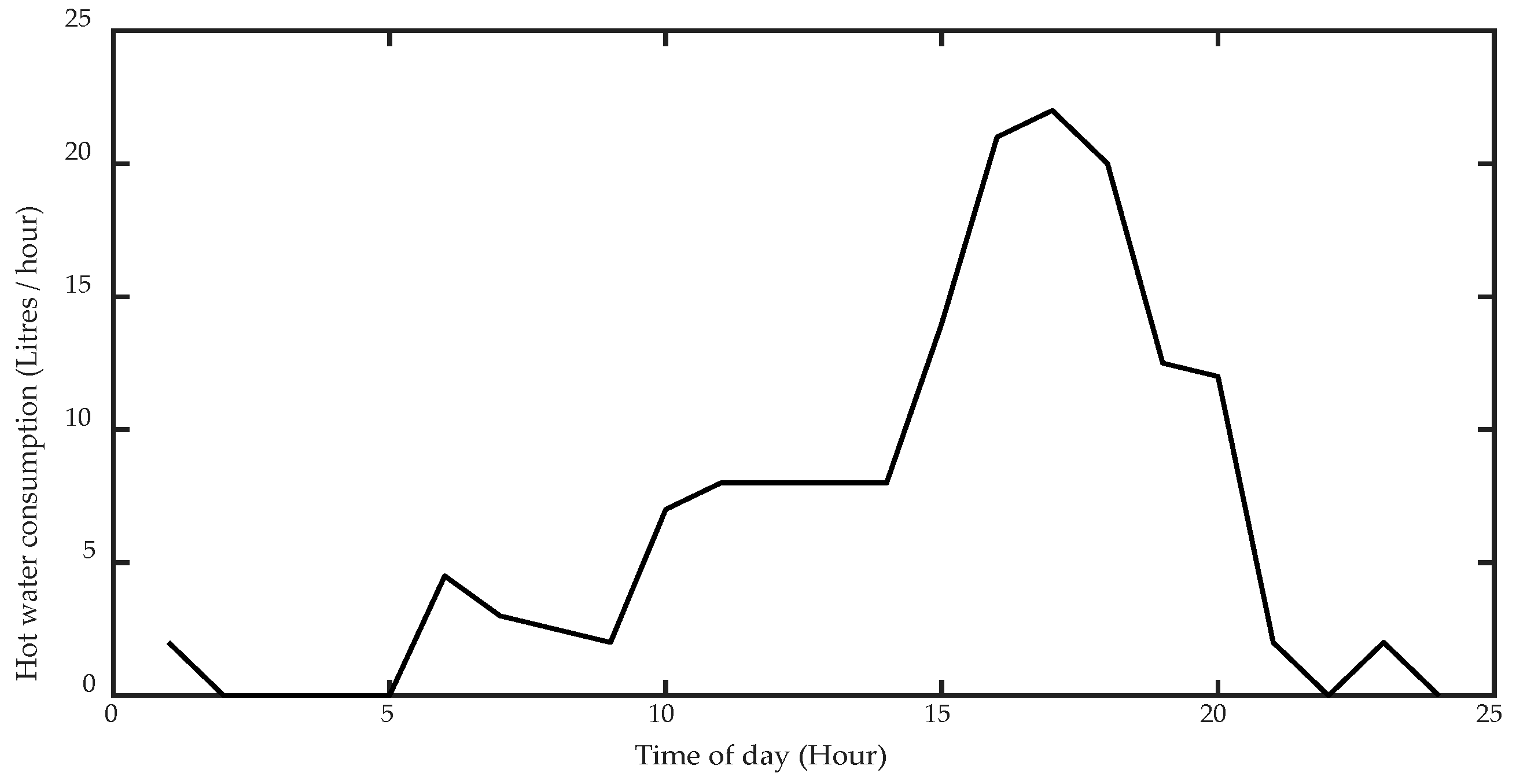
Figure 3.
Photovoltaic (PV) generation modeled for the four seasons: (a) winter; (b) spring; (c) summer; (d) autumn.
Figure 3.
Photovoltaic (PV) generation modeled for the four seasons: (a) winter; (b) spring; (c) summer; (d) autumn.

Figure 4.
Disaggregated annual residential load and external temperature.

Figure 5.
Matching indices comparison for different seasons in Case I.

Figure 6.
Load balance of the household for two typical spring days in Case II.
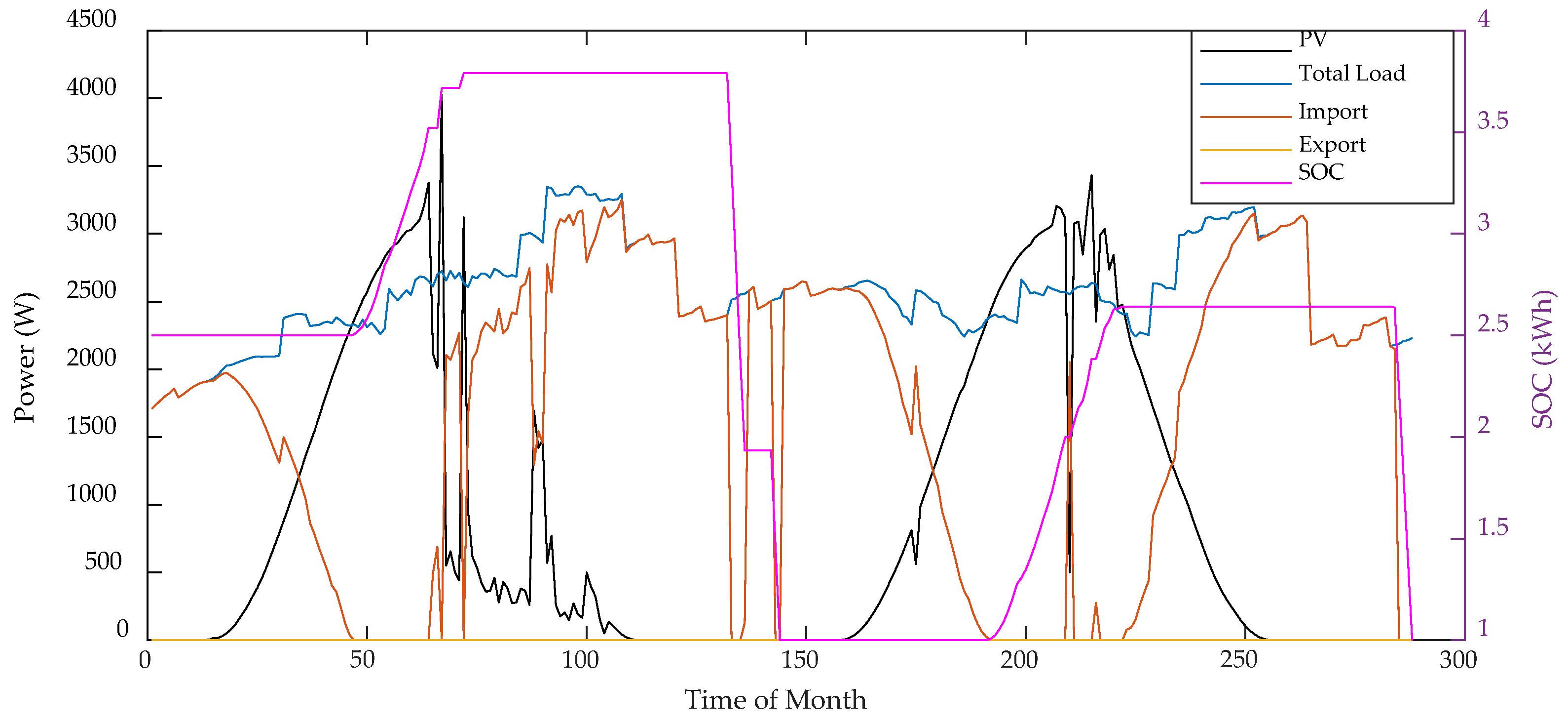
Figure 7.
Matching indices comparison for different seasons in Case II.
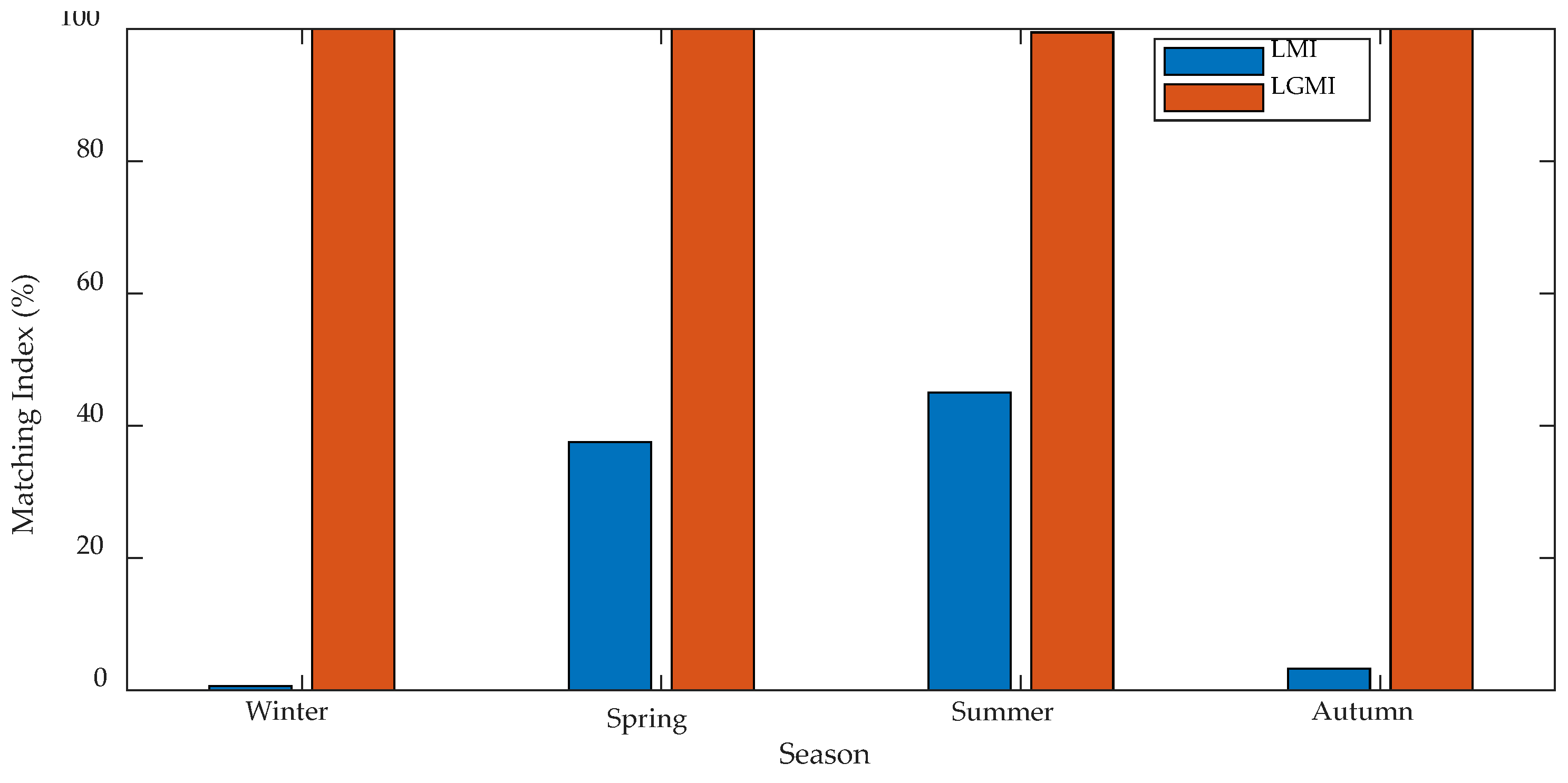
Figure 8.
Load balance of the household for two typical spring days in Case III.

Figure 9.
Matching indices comparison for different seasons in Case III.

Figure 10.
Load balance of the household for two typical spring days in Case IV.

Figure 11.
Matching indices comparison for different seasons in Case IV.
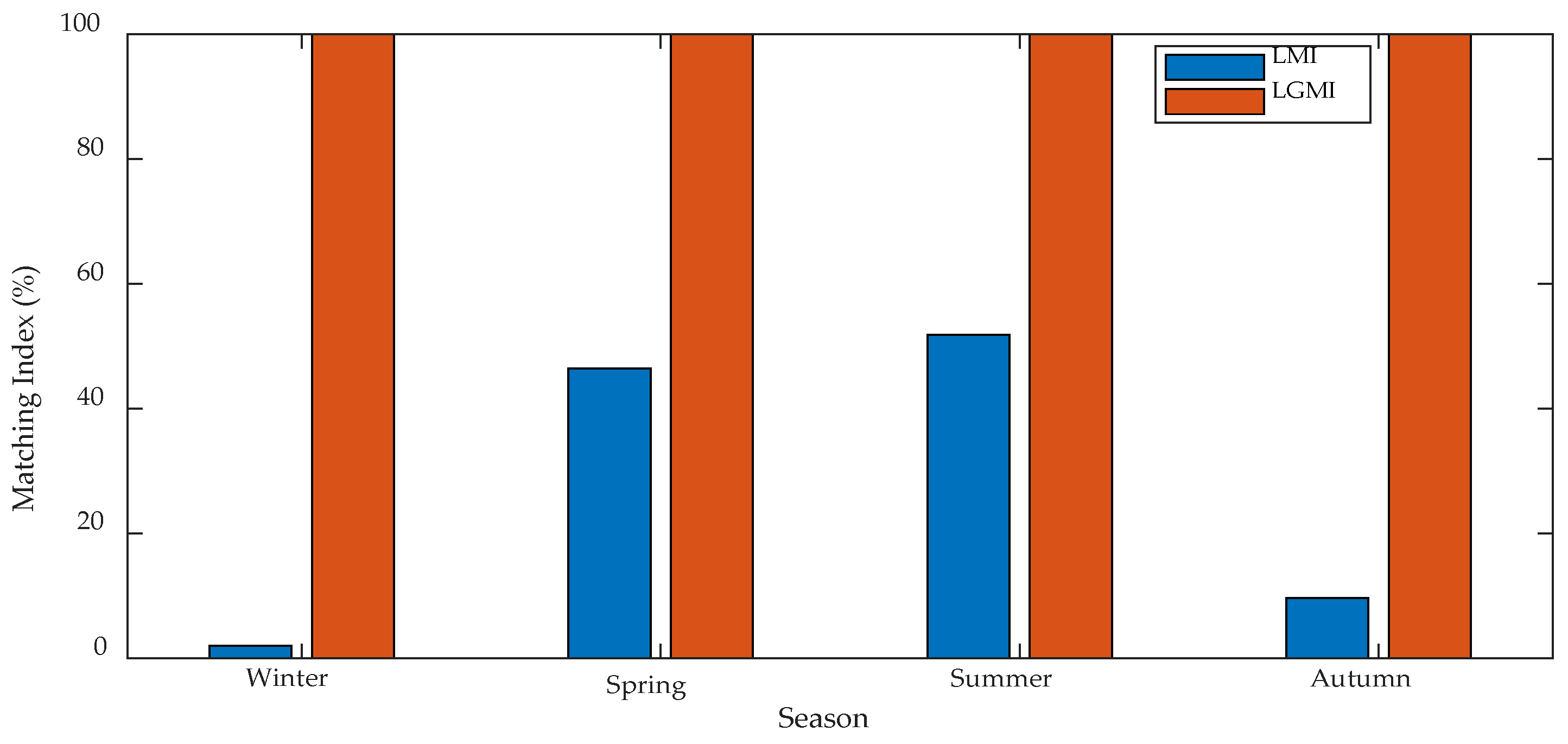
Figure 12.
Impact of increasing storage capacity on load-matching index (LMI) in Case II: (a) PVmax = 7.5 kW; (b) PVmax = 10 kW.
Figure 12.
Impact of increasing storage capacity on load-matching index (LMI) in Case II: (a) PVmax = 7.5 kW; (b) PVmax = 10 kW.

Figure 13.
Impact of increasing storage capacity on LMI in Case IV: (a) PVmax = 7.5 kW; (b) PVmax = 10 kW.
Figure 13.
Impact of increasing storage capacity on LMI in Case IV: (a) PVmax = 7.5 kW; (b) PVmax = 10 kW.


Table 1.
Two-capacity model parameters.
| Parameter | Unit | Value |
|---|---|---|
| He, Hy, Hm, Hg, Hx | W/°C | 58, 66, 1032, 10, 96 |
| Ca, Cm | W·min/°C | 217, 1868.8 |
| Tx | °C | 18 |
Table 2.
Specifications of photovoltaic (PV) module.
| Characteristic | Unit | Value |
|---|---|---|
| Model type | MAXIMA GXB 500 | |
| Rated output at standard conditions (PVmax) | W | 500 |
| Short-circuit current (Isc) | A | 9.3 |
| Module efficiency at standard conditions (η) | % | 19.3 |
| Normal operating cell temperature (NOCT) | K | 318 |
| Dimensions | mm | 1981 × 1308 × 6 |
Table 3.
Comparison of load-matching index (LMI) and local-generation-matching index (LGMI) for the case studies.
Table 3.
Comparison of load-matching index (LMI) and local-generation-matching index (LGMI) for the case studies.
| Season | Load-Matching Index (%) | Local-Generation-Matching Index (%) | ||||||
|---|---|---|---|---|---|---|---|---|
| Case I | Case II | Case III | Case IV | Case I | Case II | Case III | Case IV | |
| Winter | 0.57 | 0.63 | 1.65 | 1.96 | 100 | 100 | 100 | 100 |
| Spring | 31.79 | 37.53 | 42.6 | 46.43 | 95.82 | 100 | 100 | 100 |
| Summer | 33.72 | 45.02 | 46.73 | 51.83 | 92.7 | 99.5 | 99.51 | 100 |
| Autumn | 3.21 | 3.28 | 8.23 | 9.62 | 100 | 100 | 100 | 100 |
© 2018 by the authors. Licensee MDPI, Basel, Switzerland. This article is an open access article distributed under the terms and conditions of the Creative Commons Attribution (CC BY) license (http://creativecommons.org/licenses/by/4.0/).
Share and Cite
MDPI and ACS Style
Bashir, A.A.; Pourakbari Kasmaei, M.; Safdarian, A.; Lehtonen, M. Matching of Local Load with On-Site PV Production in a Grid-Connected Residential Building. Energies 2018, 11, 2409. https://doi.org/10.3390/en11092409
AMA Style
Bashir AA, Pourakbari Kasmaei M, Safdarian A, Lehtonen M. Matching of Local Load with On-Site PV Production in a Grid-Connected Residential Building. Energies. 2018; 11(9):2409. https://doi.org/10.3390/en11092409
Chicago/Turabian StyleBashir, Arslan Ahmad, Mahdi Pourakbari Kasmaei, Amir Safdarian, and Matti Lehtonen. 2018. "Matching of Local Load with On-Site PV Production in a Grid-Connected Residential Building" Energies 11, no. 9: 2409. https://doi.org/10.3390/en11092409
Note that from the first issue of 2016, this journal uses article numbers instead of page numbers. See further details here.