Dynamic Efficiency Analysis of an Off-Shore Hydrocyclone System, Subjected to a Conventional PID- and Robust-Control-Solution


Department of Energy Technology, Aalborg University, Esbjerg 6700, Denmark
*
Author to whom correspondence should be addressed.
†
Current address: Niels Bohrs Vej 8, Esbjerg 6700, Denmark.
Energies 2018, 11(9), 2379; https://doi.org/10.3390/en11092379
Submission received: 8 August 2018
/
Revised: 29 August 2018
/
Accepted: 5 September 2018
/
Published: 9 September 2018
Abstract
:There has been a continued increase in the load on the current offshore oil and gas de-oiling systems that generally consist of three-phase gravity separators and de-oiling hydrocyclones. Current feedback control of the de-oiling systems is not done based on de-oiling efficiency, mainly due to lack of real-time monitoring of oil-in-water concentration, and instead relies on an indirect method using pressure drop ratio control. This study utilizes a direct method where a real-time fluorescence-based instrument was used to measure the transient efficiency of a hydrocyclone combined with an upstream gravity separator. Two control strategies, a conventional PID control structure and an H robust control structure, both using conventional feedback signals were implemented, and their efficiency was tested during severely fluctuating flow rates. The results show that the direct method can measure the system’s efficiency in real time. It was found that the efficiency of the system can be misleading, as fluctuations in the feed flow affect the inlet concentration more than the outlet oil concentration, which can lead to a discharge of large oil quantities into the ocean.
1. Introduction
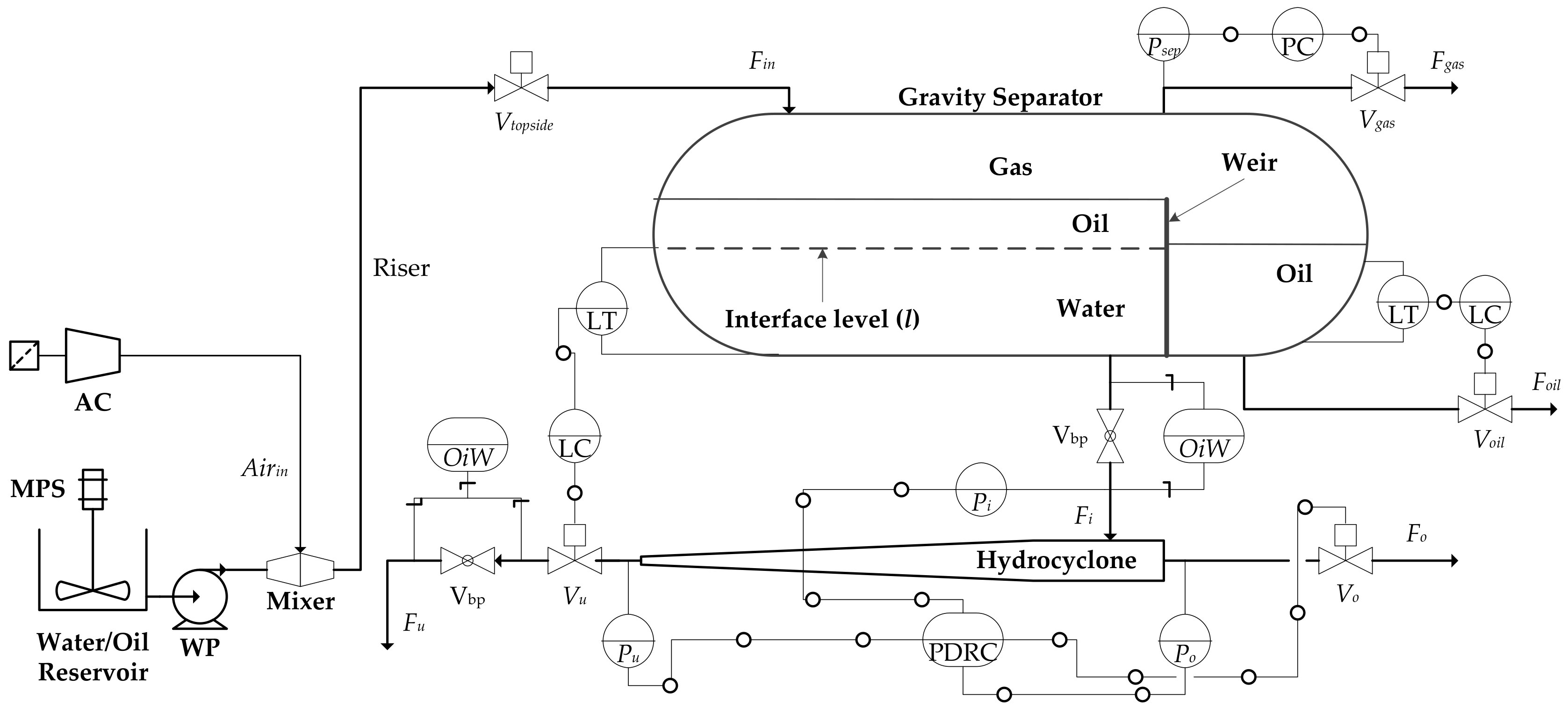
In current oil and gas production facilities, water handling is an increasing challenge, as maturing fields result in an ever-increasing water cut; in some cases up to 98% [1,2,3]. Due to high costs of equipment installation and maintenance, updates in the current facilities are preferred [4,5]. The system considered in this study is the most common type of oil and water separation facility in the Danish sector of the North Sea, consisting of a gravity separator with a downstream hydrocyclone system. The separation efficiency of the oil and water in the gravity separator is controlled by manipulating the interface level (l) of the oil and water. The manipulation of l facilitates a specific residence time that determines the separation rate of oil droplets, which then surface and get skimmed over a weir, the placement of the weir is illustrated in Figure 1. The level is governed by the underflow valve , which regulates the flow from the gravity separator () to the hydrocyclone. The separating efficiency of the hydrocyclone () is controlled by manipulating the overflow valve , which manipulates the flow of liquid through the overflow , which under the optimal operating conditions is assumed to consist of a high oil concentration. The overflow oil concentration is defined as (). This high oil concentration occurs as a centripetal force is generated due to the cylindrical shape of the hydrocyclone and the tangential injection of the liquid. The oil is thus forced to the center of the hydrocyclone forming what is known as the oil core [6,7], which is similar to the working principle of a solid–liquid hydrocyclone [7,8,9]. The feedback parameter for the control loop, is the pressure drop ratio (PDR), which is calculated using Equation (1) [10]. In previous studies, a proportionality between the PDR and the flow split has been shown, where , and is the hydrocyclone’s underflow flow rate [6,11,12,13,14]:
The PDR is thus governed by controlling , but in a previous study it was shown that negatively influences the performance of the PDR and is more dominant in comparison to [15]. The physical location of and can be seen in Figure 1. The location of the valves results in a physical coupling in the system, where has a cross-sectional area that is 25 times larger than that of and is therefore dominant with respect to the flow rate [12,16], which in turn influences the PDR.
In subsequent studies [17,18], this issue with the dominance of was addressed by updating the prevalent control strategy: currently comprising of two independent PID controllers, one for each control objective: level and PDR control. In these studies, an H robust control solution was proposed and resulted in an improved performance of the de-oiling system. In [18], reducing the fluctuation of the flow through the hydrocyclone and reducing the saturation of the control valves was believed to increase the system’s performance. The premise for this was based on previous studies [13,14,19], where it was shown through oil-in-water (OiW) measurements (manual sampling) that fluctuating flows reduced the efficiency of a hydrocyclone. The de-oiling efficiency of the hydrocyclone () is calculated through Equation (2) [20].
where is the concentration of oil in the underflow, and is the concentration of the oil in the inlet.
The determination of based on the OiW concentration has been investigated in previous studies [6,21], where relationships between the PDR and were compared to . In both studies, was investigated from a static perspective and did not deal with the dynamic changes, which is important if during fluctuating flow rates is to be investigated. This was later done in [13,22], where, in the latter study, was measured in real-time and its dynamics were observed for different operating conditions. In [22], it was observed that was not influenced by the PDR as long as PDR was kept within a specific range, which is dependent on the operating conditions. was shown to be proportional to where the proportionality was reduced as increased. This is consistent with the steady state results from [6], where increases with following an S-curve shape, and reaches steady state, which was found to be up to 99% in [6]. A potential conclusion from this is that keeping the PDR and the relatively stable within a desired operating range will result in a high . Another aspect is that relates only to the efficiency of the oil separated from the water, but it does not quantify water in the oil exiting through the overflow. This is defined as the de-watering efficiency, see Equation (3), where and are the water concentrations in the underflow and inlet, respectively. The latter is undesirable, as this results in the pollution of oil with water, which has to be handled at a cost in downstream processes or recirculation.
E is an important factor as water in the overflow will eventually have to be separated from the oil before the oil can be used, thus being a negative cost factor. In addition, as the hydrocyclone cannot achieve de-oiling efficiency (), the total amount of oil in the underflow is extremely important. For example, in 2015, the Danish oil sector discharged approximately 193 tons of dispersed oil into the sea, coming very close to the governmental limit of 202 tons [23,24].
The real-time measurement is crucial in evaluating the de-oiling performance of the hydrocyclone, which in current installations is based on manual samples and subsequent calculations performed twice a day following the OSPAR reference method [25,26]. Successful OiW measurements in the scaled pilot plant, specifically measurements of transients, have a potential for use in feedback control.
This study starts by evaluating the measurement technique used in [22] in measuring the OiW concentration in real time on the inlet and on the underflow of the hydrocyclone and extends the scope of the study by including the upstream three-phase gravity separator. The oil injection method used in [22] is in the current study replaced by an OiW mixture method that ensures a more stable OiW concentration and a more evenly distributed oil droplet size, as can be seen in Figure A1.
Using the OiW measurements, the entire system’s dynamic efficiency is evaluated during fluctuations in , where the fluctuating flow rate is crucial for several reasons. Firstly, it will enable us to evaluate if the instrument can track the transient behavior of the OiW concentration and thus the potential of using such instruments for feedback purposes. Secondly, it enables us to test the newly developed robust H control solution’s performance when subject to a disturbance, such as a fluctuating .
Two control solutions are implemented: a newly developed robust H control solution and a conventional PID control solution that is similar to the one currently used in the offshore oil and gas industry. Both controllers were developed in [18]. The goal of this is to investigate changes in the performance of by applying advanced control in comparison to a conventional control solution. The advanced control in [18] was shown to have the potential to improve the efficiency of the de-oiling system. This was based on the fact that, by reducing the impact of the fluctuation, which reverberates through the system and negatively influences , the efficiency can be improved. In the current study, this hypothesis is investigated directly through OiW measurements, thus evaluating directly.
2. Materials and Methods
2.1. Pilot Plant
The experiments were performed on a scaled pilot plant of a typical offshore de-oiling system, a simplified P&ID of this system is shown in Figure 1. Table 1 lists the description of equipment used in the pilot plant and Table 2 lists all the materials used in the experiments. The system comprises of a pump which pumps a mixture of oil and water into a mixer, where air is injected using an air compressor. This mixture is sent through a pipeline which is connected to a riser pipeline. The riser pipeline is upstream of the gravity separator, and they are separated by a topside choke valve [27,28,29]. The gravity separator is a scaled three-phase separator with a diameter of 0.6 m and an operating flow of 1 L/s (at 10 bars) and a residence time of ≈3 min, when using a weir height of 0.33 m. The gravity separator’s gas pressure is controlled using around a set point of 7 bars, which is limited by the gas pressure of the compressor. From the gravity separator, the water is sent to a single three-section 35 mm hydrocyclone liner from Vortoil [30]. The water level is measured using a differential pressure transmitter, and this measurement is used as the feedback parameter for the level control loop. The PDR is measured by the three pressure transmitters (, , and ) and is used as the feedback parameter for the PDR control loop. The liquid flows from the hydrocyclone’s overflow and underflow are controlled by the two valves ( and ), which are used in the PDR and level control loops, respectively. The OiW instruments are located at the hydrocyclone inlet and underflow, and they are referred to as in Figure 1.
2.2. The Measurement of OiW
The measurement of OiW follows the design presented in [22], where the OiW concentration is measured on the inlet and underflow of the hydrocyclone using a fluorescence based instrument, the TD-4100XDC (TD-4100) from Turner Designs. The instruments are placed on a side stream, and they are connected with a T-junction. A choke valve is used to divert some of the flow through the instruments. The instruments are calibrated to operate within a concentration range of [0–5000] ppm.
2.3. Oil-in-Water Mixture
The water and oil mixture was created by continuous stirring using two propeller stirrers to stir 2 m mixture, the propeller stirrer have a maximal capacity of 1469 m/h, but they were operated at approximately 1/3 of their maximal capacity.
A hydrocyclone’s performance is related to the droplet size at the inlet [31,32]. In order to quantify the droplet sizes in the OiW mixture, the mixture was scanned using video microscopy, using the Jorin VIPA (VIPA) instrument. The VIPA instrument was placed in the inlet side-stream and a constant flow was pumped through the system. The particles were recorded with a frame rate of 30 images/s and the particles counted using the Jorin VIPA software. For more information on the instrument refer to [33]. The droplet size distribution analysis is shown in Appendix A. The correct oil droplet distribution is difficult to evaluate, and little information on the oil droplet size distribution on the hydrocyclone inlet exists. This is because the oil droplet size distribution varies significantly between the different offshore installations and reliable measurements for offshore use have not matured. However, the general range of the droplet size has been reported to be between 1 and 1000 m in offshore untreated produced water, where most of the droplets lie in the range between 5 m and 50 m [34].
In [21], the reported droplet distribution lies between 5 and ≈120 m for a concentration of 4100 mg/L and between 3 and 70 m for a concentration of 435 mg/L. It is noteworthy that the concentration in [21] was created in the lab and is therefore not directly representative of an offshore scenario. From the histogram in Figure A1, we show that the majority of our droplets lie between 5 and 60 m, and thus we can safely say that it lies in a realistic range.
In [12], it was shown that reaching the droplet size of 60 m resulted in close to 100% efficiency. A similar result was shown in [21], where migration probability of 100% was seen when the droplet sizes were above 60 m. This indicates that, if our mixture had a significantly larger droplet size range, it would facilitate an improved separation efficiency, this could be explained as per the Stokes law, where larger droplet sizes facilitate better separation.
3. Experiment Design
A series of tests were designed to test the measurement technology and using the measurements for evaluating the performance of the control structures. The different tests are shown in Table 3 and described in the following.
3.1. Dynamic-Tracking Capability
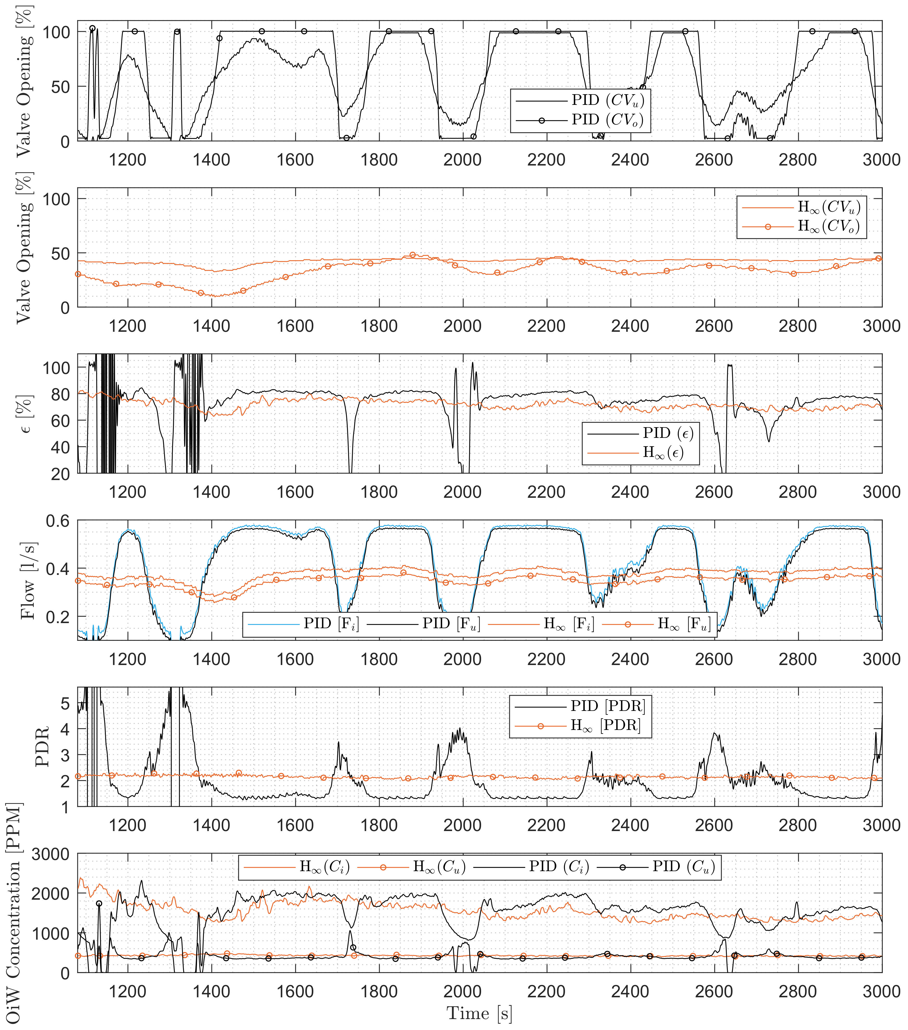
The initial experiment is a dynamic tracking capability analysis, with the objective to check whether the deployed OiW sensor could reliably track the dynamically varying flow conditions. The experiment is performed by running the PID controller at the same operating conditions two times and comparing the results. During the experiment, the system is subjected to a varying inlet flow rate, which is designed such that it emulates severe fluctuating flow rates. The fluctuating flow rates are discussed in [18,35]. The operating conditions, i.e., the inlet flow rate to the gravity separator are shown in the bottom plot in Figure 2. By varying the flow rate, it is possible to evaluate the dynamic performance of the instruments. The results are shown in the top three plots in Figure 2.
3.2. Controller Evaluation 1
The OiW measurements are evaluated on the de-oiling system, where the system is controlled using two different control strategies: (1) a PID control solution which was designed to emulate control solution from the Danish sector of the North Sea (see [18] for details) and (2) an H robust controller, which was developed in [18] and is expected to improve the system’s disturbance rejection, making the system robust towards fluctuating inlet flow rates . In this experiment, the inlet flow rate is the same as in the Dynamic-Tracking Capability experiment, which is challenging for the conventional PID control solution, and this experiment aims at investigating the two controllers disturbance rejection and de-oiling efficiency. Being able to measure the OiW concentration in real time can illuminate the benefit of using the robust controller, and we can identify the parameters that are linked to the system’s de-oiling efficiency .
3.3. Controller Evaluation 2
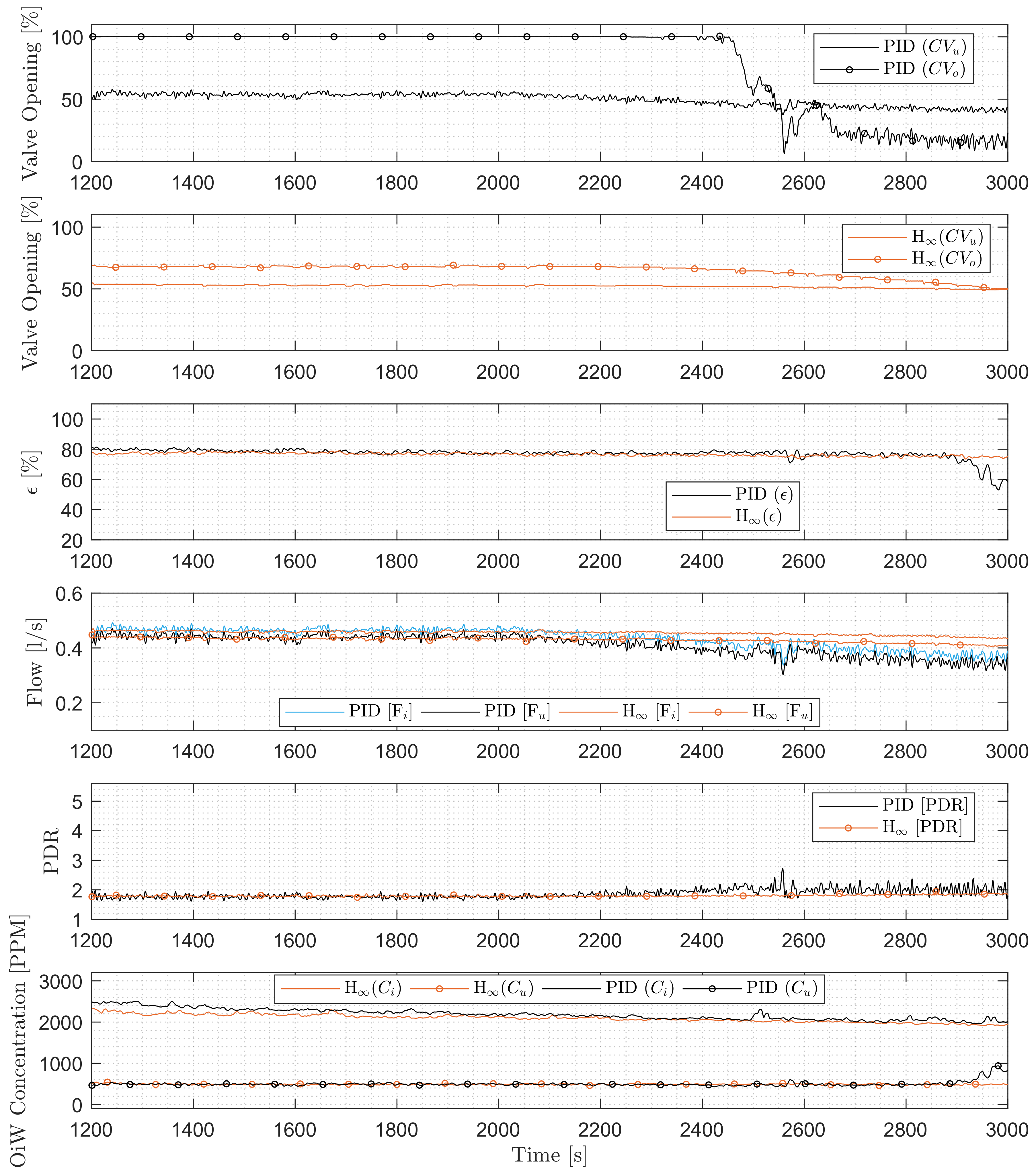
In this experiment, the system is operated first at a steady state, where the inlet flow rate is 0.47 L/s during the 1000–2000 s period. At 2000 s, the inlet flow rate is linearly decreased for 1000 s, from 0.47 to 0.37 L/s. The aim of this experiment is to investigate the system’s steady state de-oiling efficiency at different operating conditions.
4. Results and Discussion
4.1. Experiment Discussion: Dynamic-Tracking Capability
From the third plot in Figure 2, the efficiency of the two experiments appear relatively similar, except for some small deviations. The reason for the deviations are (1) a slightly alternating inlet concentration as can be seen in Plot 4 in Figure 2 and (2) the controller’s performance, which is reflected in the position of the valves in particular from 1400 to 2000 s. Nevertheless, the outlet concentration for both experiments is almost identical as seen in the bottom plot in Figure 2.
4.2. Experiment Discussion: Controller Evaluation With a Fluctuating Flow Rate
The efficiency of the hydrocyclone is calculated through Equation (2), but we find the total discharged oil concentration to be equally important, as it gives a good representation of the system’s polluting effects, in particular the total amount of discharged oil as mentioned earlier, and thus we present these results in Figure 3. The total discharged oil concentration throughout the experiment is shown in Table 4. In this initial analysis, the PID controller performs worse than the H control solution, discharging 6.95% more oil through the water. The relative larger amount of oil is related to the larger inlet flow rate, as can be seen in Figure 4, where is similar for both controllers, but is larger for the PID control solution where the total volume of the inlet mixture is 13.62% larger.
Comparing the total oil discharge to the efficiency, we see a different picture, where the PID control solution has a higher mean efficiency that the H control solution, as shown in Table 4. The higher efficiency is thought to be facilitated by the overflow valves being saturated at 100%, which occurs in many of the instances where the efficiency is above 80%. From the principles of the hydrocyclones operation [10], we can expect that, when the overflow valve is saturated at 100% opening, the flow through the overflow will be high. This causes the majority or all of the oil to flow through the overflow and thus not the underflow, which ensures good de-oiling efficiency, but at the consequence of poor de-watering separation. The negative side of this is that the overflow can potentially, in addition to the oil, contain water and thus result in poor de-watering separation . Another interesting fact is that the PID control solution returns a higher average efficiency of than the H control solution with a mean of . These results are similar to what was observed [21], where higher was observed in [6,21] while running at higher flow rates. This efficiency was achieved at a mean PDR value of 1.38, which is considered to be outside of the nominal operating range of the de-oiling hydrocyclone according to [6,13]. Instead it is more evident that the dynamic and static efficiency is more related to the inlet flow rate, as was concluded in a previous study [22].
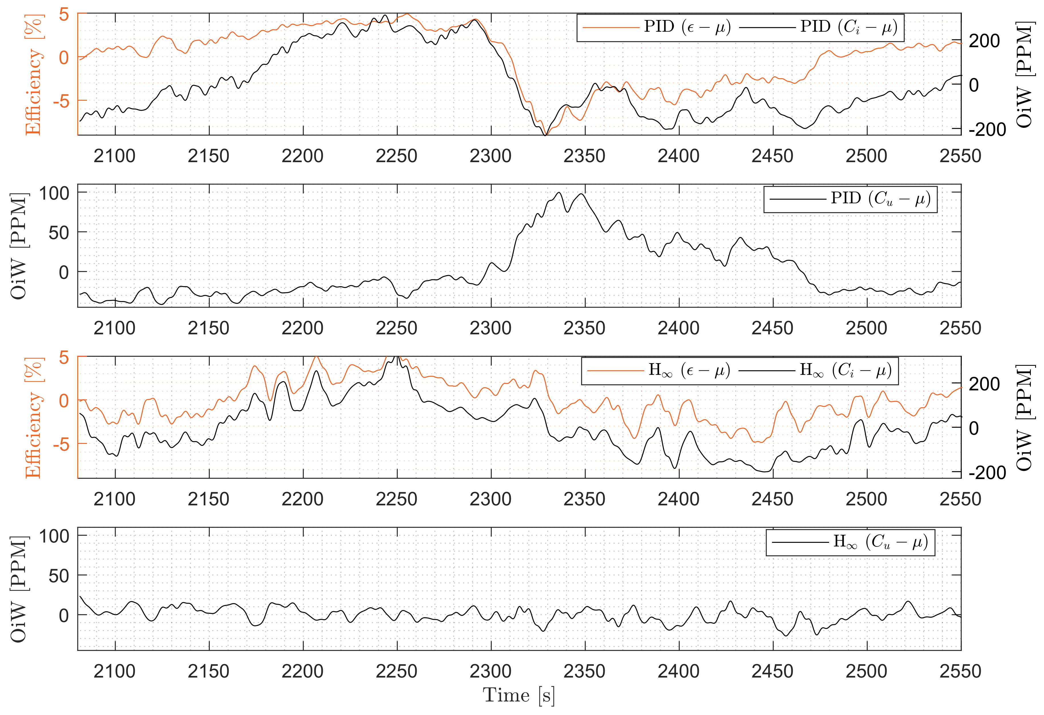
To analyze the dynamics of the efficiency in more detail, the controller evaluation experiment was investigated in a shorter time range (2050–2550 s), and the results are plotted in Figure 5. This particular range was chosen as the PID control solution results in valves to severely oscillate and influences the efficiency without reducing the efficiency to 0. A relationship between the efficiency, the underflow concentration, and the inlet concentration of the PID control solution is evident, with an inverse relationship with respect to the underflow concentration. When observing the H control solution, the is closely following the , but unlike the PID control solution the is steady, which is most likely caused by a more steady .
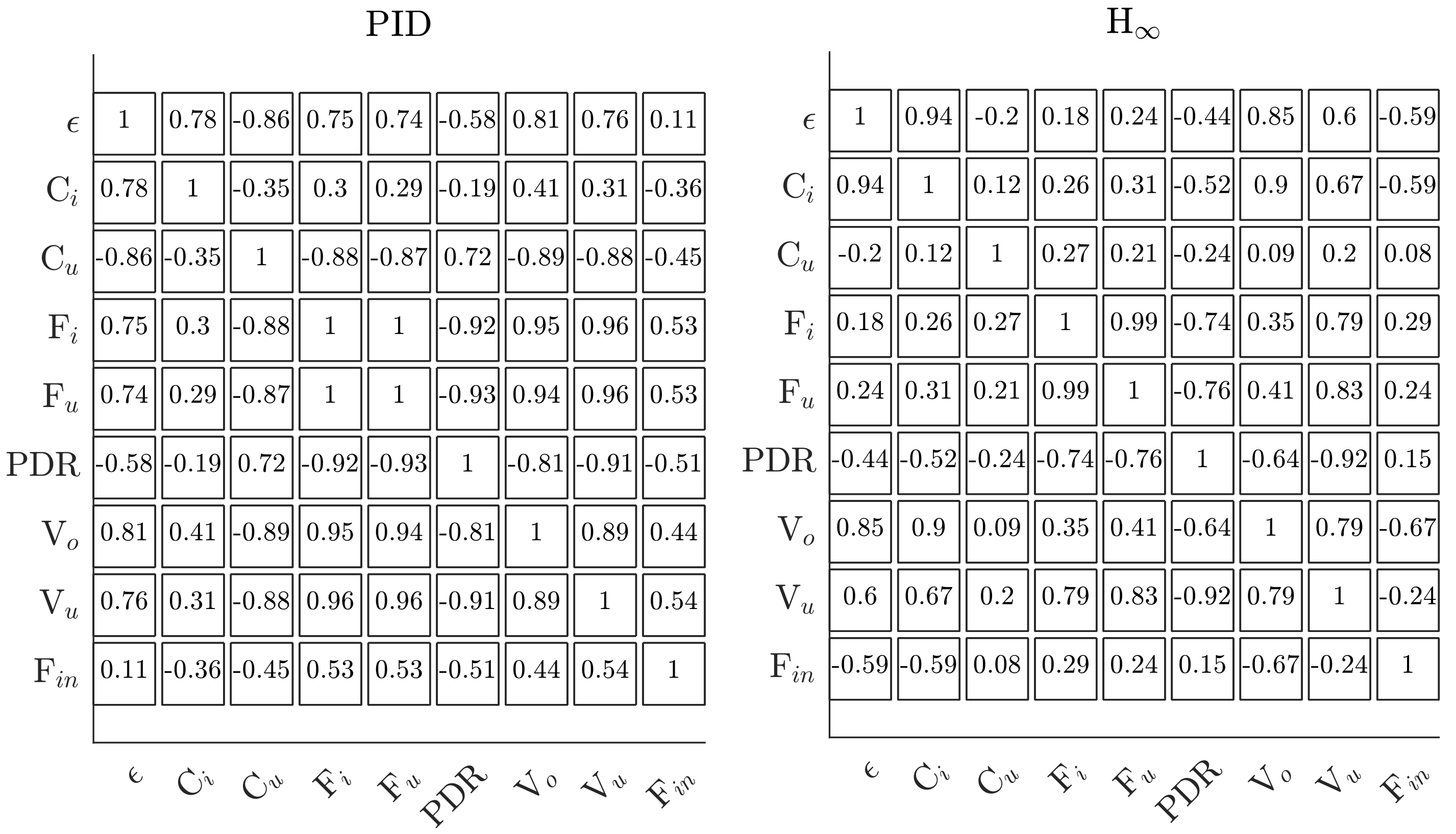
To further emphasize the relationship between the efficiency and the flow rates, a correlation coefficient has been calculated for all relevant system parameters from 2050 to 2550 s and plotted in a correlation matrix in Figure 6, where a numeric version is attached in the appendix in Figure A2. The relationship between and and that between and for the PID control solution is high, with 0.75 and 0.74 correlation coefficients, respectively, but so is the link to and , which consists of 0.78 and −0.86 correlation coefficients, respectively. This coincides with observations from Figure 5. When considering the H control solution, the lack of relationship between and is indicated by a correlation coefficient of −0.2. This value is not a true correlation but stems from the oscillations in the signals, as can be seen in Figure 5. The influence of the flow rates on is clear, as ’s relationships with both and for the H control solution present and correlation coefficients, respectively. As discussed earlier, has a significant impact on the amount of oil in the underflow, and from this analysis it can be seen that by using the H control solution is decoupled from many of the parameters, resulting in a consistent oil flow rate through the underflow during fluctuating inlet flow rates. The larger correlations between the flow and the valve actuation and between and suggest that the PID control solution leaves the hydrocyclone vulnerable towards fluctuating inlet flow rates.
4.3. Experiment Discussion: Controller Evaluation With Constant Flow Rate Followed by a Linearly Decreasing Flow Rate
Subjecting the system to a constant inlet flow rate has a positive effect on the system’s efficiency and its stability, especially when considering the PID control solution. The continuous flow into the system is reflected in the valve actuation considering the PID control solution in Figure 7, which now maintains the valves at a constant position until 2000 s, where the inlet flow rate is linearly decreasing from 0.47 to 0.37 L/s. After the linear decrease, the level controller starts to regulate the opening of , ending at an opening of . This is a good indication of the dominance of , as the relatively small change in causes a fast closing action of , which towards the end of the experiments chatters between 10 and 20%. Through the experiment, the efficiency is stable for both controllers, and so are and . After 2450 s, , with respect to the PID control solution, starts increasing due to the choking of , while remains unaffected. This directly affects . This could be an indication that the hydrocyclone’s separating mechanism is being compromised by the decreasing flow rate or that the flow of oil through the overflow is reducing; thus, an increased flow of oil is detected at the underflow. The reduced reference tracking of the robust H control solution here shows a positive effect, as the slower actuation of the valves results in a stable and thus . In cases where the inlet flow rate to the separator would be low for extensive periods, the robust H control solution would fare better than the conventional PID control solution. It is particularly in these situations, where the efficiency deviates, that OiW measurements are important, as they can be used as feedback to a controller or the operator to take the proper measures to restore maximal separation.
5. Conclusions
In this paper, we have investigated the OiW separation efficiency of a pilot scaled offshore de-oiling system consisting of a three-phase separator and a downstream hydrocyclone separator. The efficiency was measured using a novel method where two fluorescence-based oil-in-water monitors are used to measure the OiW concentration upstream and downstream of the hydrocyclone. The goal was to achieve real-time measurements of the hydrocyclones separation efficiency and investigate the potential of the measurements by the two instruments as a feedback parameter.
The system was injected with a mixture of OiW, which was stirred continuously in the buffer tank, which provided a consistent OiW concentration and droplet size distribution. Two control strategies were applied to the de-oiling system: a conventional PID control solution and a robust H control solution.
The OiW measurements were performed successfully with a good dynamic tracking capability in a wide variety of operating conditions, both with respect to steady-state and dynamic operating conditions.
In the controller evaluation, it is shown that, when the PID control solution is applied, it has a good performance while sacrificing the total oil discharge, which raises questions about the true value of . Instead, it directs more attention towards . This is especially true when the H control solution is applied, where its performance measured in is lower than that of the PID control solution, while achieving a lower and thus resulting in a lower pollutant discharge into the ocean. To elucidate, the system can perform well with respect to , while yet discharging large amounts of oil through the water fraction. In addition, the H control solution decoupled and from , which is a significant achievement, as it means that the system has become more robust towards fluctuating inlet flow rates.
Future studies will use OiW measurements in the control of the hydrocyclone, as and are the actual acclimatisation parameters, unlike the PDR or the flow split, and including them into the feedback loop will yield a better efficiency.
Author Contributions
Conceptualization, P.D. and Z.Y.; Methodology, P.D.; Software, P.D.; Validation, P.D.; Formal Analysis, P.D.; Investigation, P.D.; Resources, P.D. and Z.Y.; Writing-Original Draft Preparation, P.D.; Writing—Review & Editing, P.D. and Z.Y.; Visualization, P.D.; Supervision, Z.Y.; Project Administration, P.D. and Z.Y.
Acknowledgments
The authors would like to thank the colleagues M. Bram, D. Hansen, S. Jespersen, S. Pedersen, L. Hansen, and K. Jepsen from AAU for valuable discussions and lab support.
Conflicts of Interest
The authors declare no conflict of interest.
Abbreviations
| Name | Description | Unit |
| Inlet flow rate | L/s | |
| Separator gas outlet flow rate | m/s | |
| Hydrocyclone inlet flow rate | L/s | |
| Hydrocyclone underflow flow rate | L/s | |
| Hydrocyclone overflow flow rate | L/s | |
| Separator oil outlet flow rate | L/s | |
| Concentration of oil in the inlet | mg/L | |
| Concentration of oil in the underflow | mg/L | |
| Concentration of oil in the overflow | mg/L | |
| Concentration of water in the underflow | mg/L | |
| Concentration of water in the overflow | mg/L | |
| Separator pressure | bar | |
| Hydrocyclone inlet pressure | bar | |
| Hydrocyclone underflow pressure | bar | |
| Hydrocyclone overflow pressure | bar | |
| PDR | Hydrocyclone pressure drop ratio | - |
| Topside choke valve | % | |
| Separator gas outlet valve | % | |
| Separator oil outlet valve | % | |
| Hydrocyclone underflow valve | % | |
| Hydrocyclone overflow valve | % | |
| OIW instrument bypass valve | % | |
| OiWT | Oil-in-water transmitter | mg/L |
| OiW | Oil-in-water | - |
| Hydrocyclones de-oiling efficiency | % | |
| E | Hydrocyclones de-watering efficiency | % |
Appendix A. Analysis of the OiW Mixture’s Droplet Size Distribution
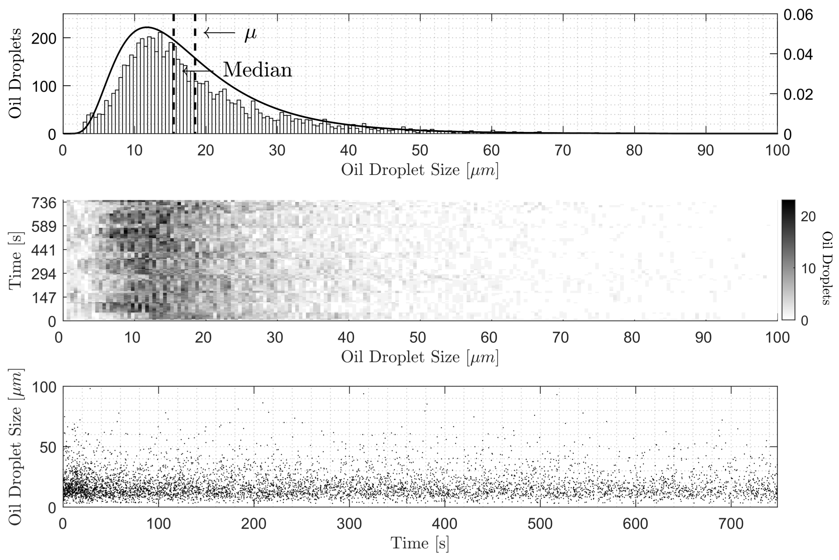
The oil-in-water mixture was analyzed using video microscopy, with the Jorin VIPA particle analyzer. In total, 15,000 images were recorded over the span of 748 seconds and analyzed. In this period, 6347 oil droplets were recognized by the software, based on a shape factor of 0.8, where the shape factor is calculated based on Equation (A1) and the droplet size is calculated based on the average Feret diameter [33,36,37].
The oil droplet distribution, shown in Figure A1, indicates droplets in the range from 3.0249 to 102.8636 m, with a mean and median of 18.4737 m and 15.4722 m, respectively. To analyze the stability of the oil droplet distribution, a moving window histogram, with a window size of 500 samples, is shown in the second plot in Figure A1. Finally, in the bottom plot, the raw data is plotted as a reference.
Figure A1.
Histogram of the droplet sizes with a fitted log normal distribution. The bottom plot shows all the detected droplet sizes with a linear fit.
Figure A1.
Histogram of the droplet sizes with a fitted log normal distribution. The bottom plot shows all the detected droplet sizes with a linear fit.

Appendix B. Correlation Analysis
The correlation matrix shown in Figure A2 is the same as shown in Figure 6, where the color scheme has been replaced with numerical values.
Figure A2.
Correlation matrix of system parameters for the 2080–2550 s time period, with respect to the PID and H control solution. Here shown with numerical values.
Figure A2.
Correlation matrix of system parameters for the 2080–2550 s time period, with respect to the PID and H control solution. Here shown with numerical values.
References
- Stephenson, M. A survey of produced water studies. In Produced Water; Springer: Boston, MA, USA, 1992. [Google Scholar]
- Bailey, B.; Crabtree, M.; Tyrie, J.; Elphick, J.; Kuchuk, F.; Romano, C.; Roodhart, L. Water control. Oilfield Rev. 2000, 12, 30–51. [Google Scholar]
- Veil, J.A.; Puder, M.G.; Elcock, D.; Redweik, R.J., Jr. A white paper describing produced water from production of crude oil, natural gas, and coal bed methane. Argonne Nat. Lab. Tech. Rep. 2004, 63. [Google Scholar] [CrossRef]
- Peel, J.; Howarth, C.; Ramshaw, C. Process intensification: Higee seawater deaeration. Chem. Eng. Res. Des. 1998, 76, 585–593. [Google Scholar] [CrossRef]
- Emmerson. Reducing Size in Offshore Topsides Valve Automation. 2018. Available online: http://www2.emersonprocess.com/en-US/brands/bettis/featuredSolutions/Pages/bettisSY.aspx (accessed on 19 February 2018).
- Meldrum, N. Hydrocyclones: A Solution to Produced-Water Treatment. SPE Prod. Eng. 1988, 3, 669–676. [Google Scholar] [CrossRef]
- Svarovsky, L. Solid-liquid Separation; Elsevier: Oxford, UK, 2000. [Google Scholar]
- Svarovsky, L. Hydrocyclones. In Solid-Liquid Separation; Elsevier: Oxford, UK, 2001; pp. 191–245. [Google Scholar]
- Svarovsky, L.; Thew, M. Hydrocyclones: Analysis and Applications; Springer Science & Business Media: Berlin, Germany, 2013. [Google Scholar]
- Thew, M. Hydrocyclone redesign for liquid-liquid separation. Chem. Eng. 1986, 427, 17–23. [Google Scholar]
- Thew, M.; Silk, S.; Colman, D. Determination and use of residence time distributions for two hydrocyclones. In Proceedings of the International Conference on Hydrocyclones, Churchill College, Cambridge, UK, 1–3 October 1980. [Google Scholar]
- Young, G.; Wakley, W.; Taggart, D.; Andrews, S.; Worrell, J. Oil-water separation using hydrocyclones: An experimental search for optimum dimensions. J. Pet. Sci. Eng. 1994, 11, 37–50. [Google Scholar] [CrossRef]
- Husveg, T.; Rambeau, O.; Drengstig, T.; Bilstad, T. Performance of a deoiling hydrocyclone during variable flow rates. Min. Eng. 2007, 20, 368–379. [Google Scholar] [CrossRef]
- Husveg, T. Operational Control of Deoiling Hydrocyclones and Cyclones for Petroleum Flow Control. Ph.D. Thesis, University of Stavanger, Stavanger, Norway, 2007. [Google Scholar]
- Durdevic, P.; Pedersen, S.; Yang, Z. Challenges in Modelling and Control of Offshore De-oiling Hydrocyclone Systems. J. Phys. Conf. Ser. 2017, 783. [Google Scholar] [CrossRef]
- Wolbert, D.; Ma, B.F.; Aurelle, Y.; Seureau, J. Efficiency estimation of liquid-liquid Hydrocyclones using trajectory analysis. AIChE J. 1995, 41, 1395–1402. [Google Scholar] [CrossRef]
- Durdevic, P. Real-Time Monitoring and Robust Control of Offshore De-oiling Processes. Ph.D. Thesis, Aalborg University, Aalborg, Denmark, 2017. [Google Scholar]
- Durdevic, P.; Yang, Z. Application of H∞ Robust Control on a Scaled Offshore Oil and Gas De-Oiling Facility. Energies 2018, 11, 287. [Google Scholar] [CrossRef]
- Husveg, T.; Johansen, O.; Bilstad, T. Operational Control of Hydrocyclones During Variable Produced Water Flow Rates—Frøy Case Study. SPE Prod. Oper. 2007, 22, 294–300. [Google Scholar]
- Thew, M.T. Cyclones for oil/water separation. In Encyclopaedia of Separation Science, 4th ed.; Academic Press: Cambridge, MA, USA, 2000; pp. 1480–1490. [Google Scholar]
- Simms, K.; Zaidi, S.; Hashmi, K.; Thew, M.; Smyth, I. Testing of the vortoil deoiling hydrocyclone using Canadian offshore crude oil. In Hydrocyclones; Springer: Dordrecht, The Netherlands, 1992; pp. 295–308. [Google Scholar]
- Durdevic, P.; Raju, C.S.; Bram, M.V.; Hansen, D.S.; Yang, Z. Dynamic Oil-in-Water Concentration Acquisition on a Pilot-Scaled Offshore Water-Oil Separation Facility. Sensors 2017, 17, 124. [Google Scholar] [CrossRef] [PubMed]
- Miljoestyrelsen. Generel Tilladelse for Mærsk Olie og Gas A/S (Mærsk Olie) Tilanvendelse, Udledning Oganden Bortskaffelse af Stoffer og Materialer, Herunder Olie og Kemikalier i Produktions-og Injektionsvand Fraproduktionsenhederne Halfdan, Dan, Tyra og Gorm for Perioden 1. Januar 2017–31. December 2018. Available online: https://mst.dk/media/92144/20161221-ann-generel-udledningstilladelse-for-maersk-olie-og-gas-2017-18.pdf (accessed on 12 June 2018).
- Hall, O.; SchrØder, C. Mærsk Afviser Kritik: Vores Olieforurening er Minimal. 2018. Available online: https://www.dr.dk/nyheder/penge/maersk-afviser-kritik-vores-olieforurening-er-minimal (accessed on 7 September 2018).
- OSPAR Commission, about OSPAR. 2018. Available online: https://www.ospar.org/about (accessed on 10 January 2018).
- Methodology for the Sampling and Analysis of Produced Water and Other Hydrocarbon Discharges. 2016. Available online: https://www.gov.uk/guidance/oil-and-gas-offshore-environmental-legislation (accessed on 3 November 2016).
- Storkaas, E.; Skogestad, S.; Godhavn, J.M. A low-dimensional dynamic model of severe slugging for control design and analysis. In Proceedings of the 11th International Conference on Multiphase Flow (Multiphase03), San Remo, Italy, 11–13 June 2003; pp. 117–133. [Google Scholar]
- Ogazi, A.I. Multiphase Severe Slug Flow Control. Ph.D. Thesis, Cranfield University, Cranfield, UK, 2011. [Google Scholar]
- Yang, Z.; Stigkær, J.P.; Løhndorf, B. Plant-wide control for better de-oiling of produced water in offshore oil & gas production. IFAC-papersonline 2013, 3, 45–50. [Google Scholar] [CrossRef]
- VORTOIL Deoiling Hydrocyclones. 2018. Available online: http://www.slb.com/~/media/Files/processing-separation/product-sheets/vortoil-ps.pdf (accessed on 5 July 2018).
- Rietema, K.; Maatschappij, S.I.R. Performance and design of hydrocyclones—III: Separating power of the hydrocyclone. Chem. Eng. Sci. 1961, 15, 310–319. [Google Scholar] [CrossRef]
- Bram, M.V.; Hansen, L.; Hansen, D.S.; Yang, Z. Hydrocyclone Separation Efficiency Modeled by Flow Resistances and Droplet Trajectories. IFAC-papersonline 2018, 51, 132–137. [Google Scholar] [CrossRef]
- Nezhati, K.; Roth, N.; Gaskin, R. “On-line determination of particle size and concentration (solids and oil) using ViPA Analyser-A way forward to control subsea separators ”presented at the IBC Production Separation Systems Conference. In Proceedings of the 7th Annual International Forum-Production Separation Systems, London, UK, 13–14 June 2001. [Google Scholar]
- Bradley, H.B. Petroleum Engineering Handbook; U.S. Department of Energy Office of Scientific and Technical Information (OSTI): Washington, DC, USA, 1987.
- Hansen, L.; Durdevic, P.; Jepsen, K.L.; Yang, Z. Plant-wide Optimal Control of an Offshore De-oiling Process Using MPC Technique. IFAC-PapersOnLine 2018, 51, 144–150. [Google Scholar] [CrossRef]
- Yang, M. Measurement of oil in produced water. In Produced Water; Springer: New York, NY, USA, 2011. [Google Scholar]
- Jorin Particle Detection. 2018. Available online: http://www.jorin.co.uk/technology/detection/ (accessed on 14 June 2018).
Figure 1.
Simplified P&ID of the pilot plant.

Figure 2.
Experiment Results: Dynamic-Tracking Capability analysis; results of two experiments and performed under the same operating conditions using the same PID control solution; the plots show valve openings, efficiencies, OiW concentrations, and .
Figure 2.
Experiment Results: Dynamic-Tracking Capability analysis; results of two experiments and performed under the same operating conditions using the same PID control solution; the plots show valve openings, efficiencies, OiW concentrations, and .
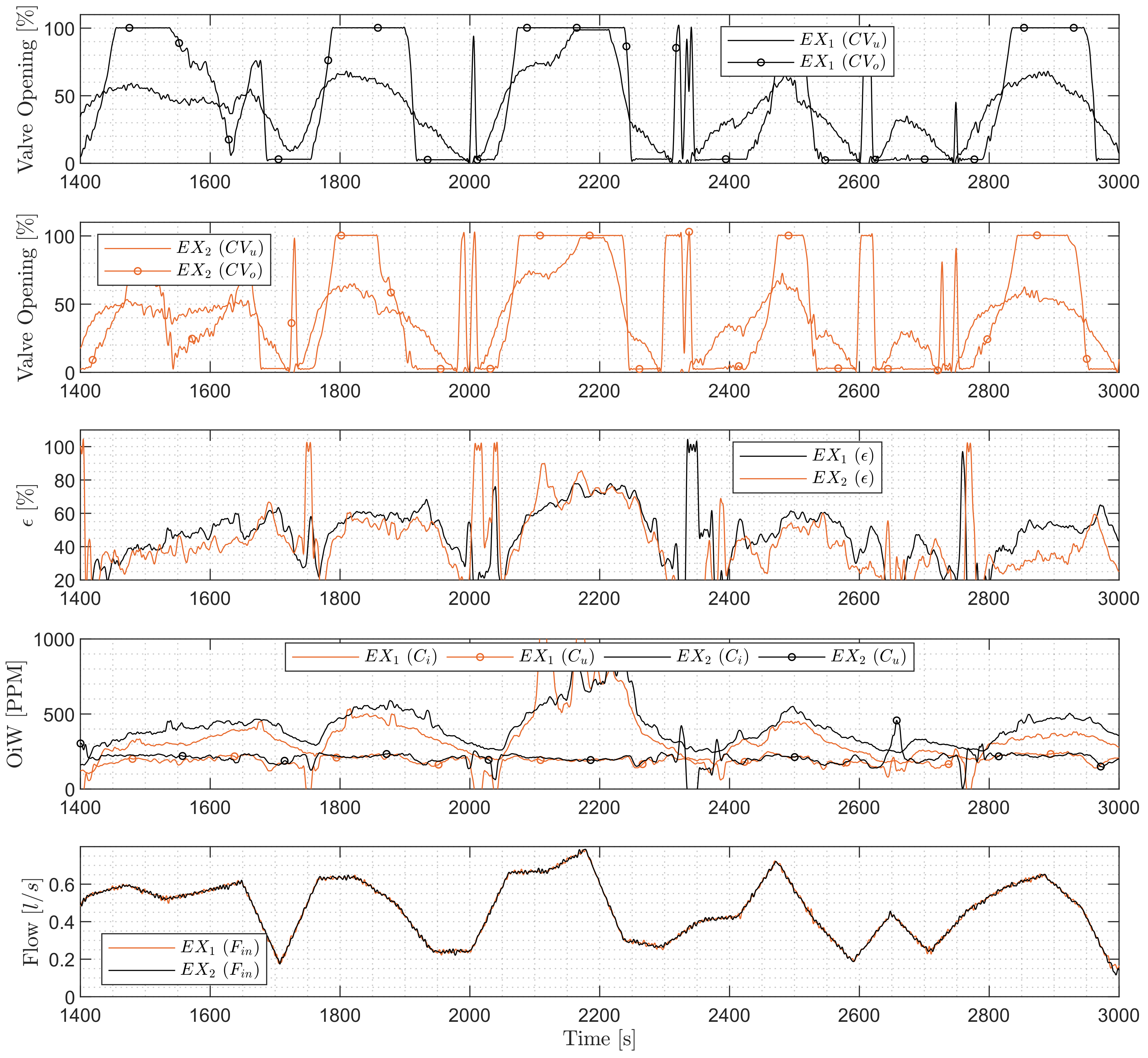
Figure 3.
Experiment Results: controller evaluation with fluctuating inlet flow rate . This plot shows the total oil discharged through the underflow.
Figure 3.
Experiment Results: controller evaluation with fluctuating inlet flow rate . This plot shows the total oil discharged through the underflow.
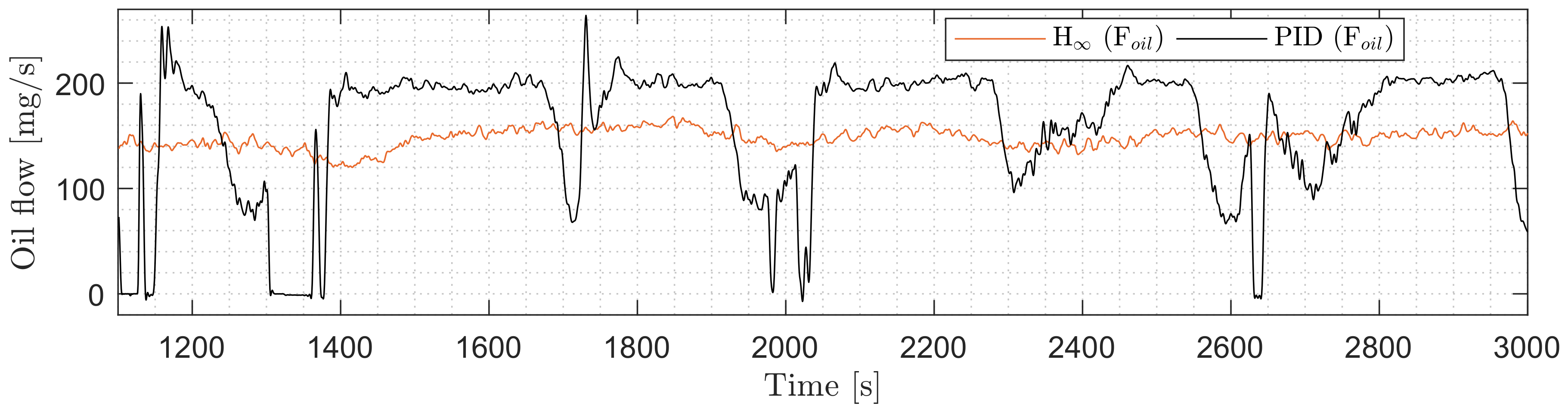
Figure 4.
Experiment Results: controller evaluation with fluctuating inlet flow rate . The plots show valve openings, efficiencies, flows, PDRs, and OiW concentrations.
Figure 4.
Experiment Results: controller evaluation with fluctuating inlet flow rate . The plots show valve openings, efficiencies, flows, PDRs, and OiW concentrations.

Figure 5.
Experiment Results: controller evaluation with fluctuating flow rate, zoomed in on a portion of the experiment to show the dynamics of the OiW measurements. The mean has been subtracted to emphasize the dynamic relationship.
Figure 5.
Experiment Results: controller evaluation with fluctuating flow rate, zoomed in on a portion of the experiment to show the dynamics of the OiW measurements. The mean has been subtracted to emphasize the dynamic relationship.

Figure 6.
Correlation matrix of system parameters from 2080 to 2550 s, with respect to the PID and H control solution. A numerical version is attached in the appendix, see Figure A2.
Figure 6.
Correlation matrix of system parameters from 2080 to 2550 s, with respect to the PID and H control solution. A numerical version is attached in the appendix, see Figure A2.
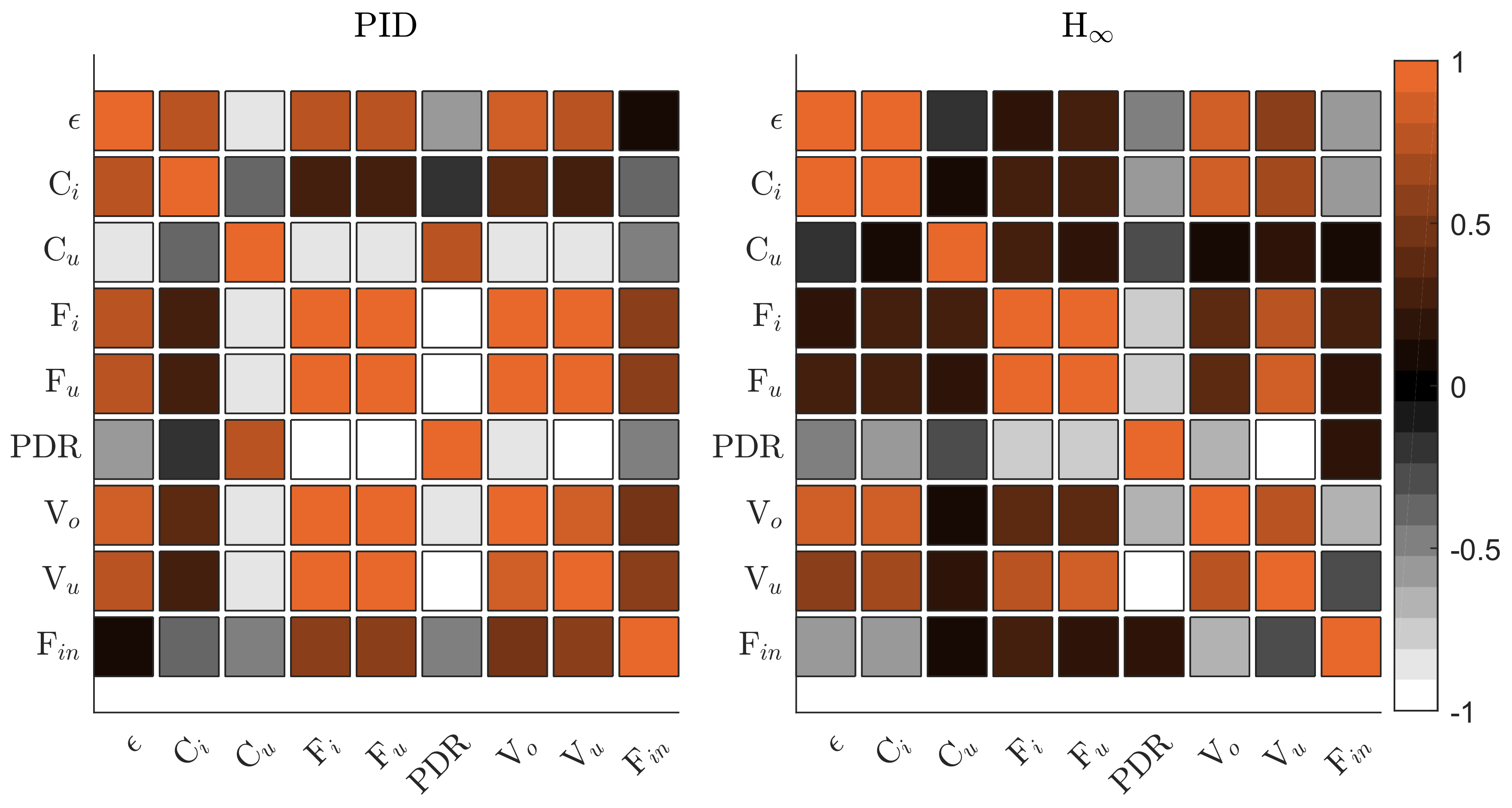
Figure 7.
Experiment Results: controller evaluation with constant inlet flow rate at 1000–2000 s at 0.47 L/s, followed by a linearly decreasing flow, from 0.47 to 0.37 L/s, 2000–3000 s. The plots show valve openings, efficiencies, flows, PDRs, and OiW concentrations.
Figure 7.
Experiment Results: controller evaluation with constant inlet flow rate at 1000–2000 s at 0.47 L/s, followed by a linearly decreasing flow, from 0.47 to 0.37 L/s, 2000–3000 s. The plots show valve openings, efficiencies, flows, PDRs, and OiW concentrations.


Table 1.
Description of the instruments and equipment used for the de-oiling set-up.
| Name | Type | Description | Range/size |
|---|---|---|---|
| WP | Grundfos CRNE 3 | Centrifugal water feed pump | 1 L/s at 162.7 m, max 25 bar |
| H | Vortoil liner | Up to 2 industrial hydrocyclone liners | 1.4” |
| Siemens Sitrans P200 | Piezo-resistive pressure measuring cell | (0–16) bar | |
| AC | — | Air compressor | 8.5 bar |
| LT | Rosemount 3051SAL | Scalable Level Transmitter | 6 mHO @4C-g |
| Rosemount 8732 | Electromagnetic flow transmitter | DN50 (0–25.97) L/s @ 12 m/s | |
| Bailey-Fischer-Porter 10DX4311C | Electromagnetic flow transmitter | DN15 (0–1.64) L/s | |
| Micro-Motion Coriolis Elite (CMFS010) | Coriolis flow transmitter | DN10 L/s | |
| Turner-Design TD-4100XDC | Fluorescence measurement OiW monitor | (0 ppb–5000 ppm) | |
| MPS | Milton Roy Mixing, 77212 AVON Cedex, FRANCE | Motorized Propeller Stirrer | 750/h, 1.1 KW, 137 RPM, Propeller D = 550 mm |
| Tank | Custom made | Stainless steel tank | 3 m |
| Bürkert 2301+8696 | Pneumatic Globe valve | mm mm | |
| Bürkert 2301+8696 | Pneumatic Globe valve | mm mm | |
| Bürkert 8626 | Mass flow controller | 20–1500 /min, @ 1.013 bar and 0 C |
Table 2.
Description of chemicals used for the hydrocyclone set-up.
| Name | Type | Description | Company |
|---|---|---|---|
| Oil | MIDLAND NON DETERGENT 30 | SAE 30 API SB | Oel-Brack AG |
| Air | From compressor | ≈8 bars | – |
| Water | From tap | ≈23.5 C | – |
Table 3.
List of experiments performed in this paper.
| Experiment Name | Aim |
|---|---|
| Dynamic-Tracking Capability | Evaluate the instruments dynamic and static performance |
| Controller Evaluation 1 | Evaluate the de-oiling efficiency () during fluctuating flow |
| Controller Evaluation 2 | Evaluate the instruments dynamic and static performance |
Table 4.
Total volume of the inlet mixture, total volume of oil discharged, and mean de-oiling efficiency . In the experiment (controller evaluation with fluctuating inlet flow rate ), the duration was 1900 s.
Table 4.
Total volume of the inlet mixture, total volume of oil discharged, and mean de-oiling efficiency . In the experiment (controller evaluation with fluctuating inlet flow rate ), the duration was 1900 s.
| Controller | Amount | Unit |
|---|---|---|
| PID control solution [] | 827.46 | L |
| H control solution [] | 714.73 | L |
| PID control solution [] | 0.302 | kg |
| H control solution [] | 0.281 | kg |
| PID control solution [] | 78.92 | % |
| H control solution [] | 71.8 | % |
© 2018 by the authors. Licensee MDPI, Basel, Switzerland. This article is an open access article distributed under the terms and conditions of the Creative Commons Attribution (CC BY) license (http://creativecommons.org/licenses/by/4.0/).
Share and Cite
MDPI and ACS Style
Durdevic, P.; Yang, Z. Dynamic Efficiency Analysis of an Off-Shore Hydrocyclone System, Subjected to a Conventional PID- and Robust-Control-Solution. Energies 2018, 11, 2379. https://doi.org/10.3390/en11092379
AMA Style
Durdevic P, Yang Z. Dynamic Efficiency Analysis of an Off-Shore Hydrocyclone System, Subjected to a Conventional PID- and Robust-Control-Solution. Energies. 2018; 11(9):2379. https://doi.org/10.3390/en11092379
Chicago/Turabian StyleDurdevic, Petar, and Zhenyu Yang. 2018. "Dynamic Efficiency Analysis of an Off-Shore Hydrocyclone System, Subjected to a Conventional PID- and Robust-Control-Solution" Energies 11, no. 9: 2379. https://doi.org/10.3390/en11092379
Note that from the first issue of 2016, this journal uses article numbers instead of page numbers. See further details here.