Simulation of Fluid-Thermal Field in Oil-Immersed Transformer Winding Based on Dimensionless Least-Squares and Upwind Finite Element Method

Abstract

In order to study the coupling fluid and thermal problems of the local winding in oil-immersed power transformers, the least-squares finite element method (LSFEM) and upwind finite element method (UFEM) are adopted, respectively, to calculate the fluid and thermal field in the oil duct. When solving the coupling problem by sequential iterations, the effect of temperature on the material property and the loss density of the windings should be taken into account. In order to improve the computation efficiency for the coupling fields, an algorithm, which adopts two techniques, the dimensionless LSFEM and the combination of Jacobi preconditioned conjugate gradient method (JPCGM) and the two-side equilibration method (TSEM), is proposed in this paper. To validate the efficiency of the proposed algorithm, a local winding model of a transformer is built and the fluid field is computed by the conventional LSFEM, dimensionless LSFEM, and the Fluent software. While the fluid and thermal computation results of the local winding model of a transformer obtained by the two LSFEMs are basically consistent with those of the Fluent software, the stiffness matrix, which is formed by the dimensionless scheme of LSFEM and preconditioned by the JPCGM and TSEM, has a smaller condition number and a faster convergence rate of the equations. Thus, it demonstrates a broader applicability.

1. Introduction

As the core equipment of power systems, power transformers are usually used for power transfer and voltage alternating, and its reliable operation is the premise to guarantee the quality of the power supply. Therefore, manufacturers and researchers are continuously committed to improving their performance and prolonging their life expectancy [1]. The service life of a transformer is dictated mainly by the aging of the paper insulation, which is affected in turn by the maximum temperatures in the various components during its operation. During the operation of the transformer, a small portion of the electrical energy gets lost in the form of heat during the transmission. For the forced oil circulation, the cold oil is pumped into the transformer through the inlet by the oil pump and contacts the heat generating components such as the iron core and windings through the oil duct; it absorbs the heat and then flows out of the tank through the outlet. For the nature oil circulation, the hot oil, which contacts the inner wall of the tank, flows upward after absorbing the heat and then transfers it to the tank; the tank transfers heat to air in the end. After cooling, the oil flows downward. Due to the convective circulation of oil, a closed loop is formed. In short, acting as the medium of heat transfer, the oil is the most important part of the cooling system in transformers [2,3]. If the cooling system is not designed appropriately, the overheating phenomenon of the components will occur [4,5,6]. As mentioned in Reference [7], in the hotspot, the depolymerization process of cellulose insulation gradually emerges, which will degrade the mechanical properties of cellulose paper, such as tensile strength and elasticity, and makes the paper brittle and incapable of enduring electrical forces and vibrations. This irreversible deterioration strongly affects the transformers service life. To ensure the normal operation of the transformer, the temperature must be kept below a critical level by effectively dissipating the generated heat [8,9]. The use of oil as insulation material has proven to be very efficient in dissipating the heat and it displays unique dielectric properties as well, which makes the oil immersed cooling type of power transformer widely applied in high voltage power transmission systems. Since the flow distribution in the cooling channel directly affects the operation temperature, the adoption of proper cooling systems is critical to the thermal management of transformers [10]. To get a better understanding of the thermal behavior and to optimize the thermal performance of oil-immersed transformers, the characteristics of oil flow velocity and temperature distribution has been analyzed and discussed by numerical simulations techniques [11,12,13,14,15,16,17,18,19,20,21,22,23,24,25,26,27].

Torriano et al., [10] numerically studied the impacts of the operational parameters, such as the mass flow rate and boundary conditions on the flow and temperature distributions of the windings. As can be concluded, the higher the flow rate, the better cooling effect of the windings can be achieved. With a more uniform temperature distribution in the windings, the hotspot temperature decreases. Kranenborg et al., [12] conducted computational fluid dynamics (CFD) simulations on a winding consisting of six partitions. They noted that the formation of hot streaks in the fluid and recognized their great influence on the downstream temperature distribution. In the literature in Reference [10], Skillen et al., [13] conducted a more detailed study on predicting the mixed-convection flow of coolant in a low-voltage transformer winding. They explored the generation mechanism of hot streaks and also found that there is a strong coupling among the flows in different passes. The experimental devices of the local winding, the transformer slicing model, and the entire structure of the transformer was established in the literature in Reference [20,21,22,23], respectively. The thermal profile of a transformer was experimentally investigated from different levels of complexity. Godina et al., [24] made a comprehensive review by analyzing and discussing the existing studies on the effect of loads and other key factors on oil-transformer ageing. They analyzed each relevant factor in detail and concluded that a monitoring system is essential to ensure the reliable operation of a transformer. Ramos et al., [25] has developed a mathematical differential model to represent the ventilation and the thermal performance of underground transformer substations, and numerically solved it. By the simulations of the model, whose validity has been verified by the temperature rise test, two important parameters related to the ventilation performance of the substation were obtained. Recently, some researchers have combined the response surface optimization method with the numerical calculation method to optimize the design of the transformer cooling system [7,27]. Zhang et al., [27] constructed a 3-D computational fluid dynamic model for a transformer to generate the training data for response surface method (RSM). They employed two types of RSMs to evaluate their performance of designed cooling systems. A comparison of the solution and the results obtained by the direct optimization method was conducted to verify the effectiveness of the RSM in the design of an oil-immersed transformer cooling system. Raeisian et al., [7] developed a numerical scheme to examine the effective parameters on the thermal management of distribution transformers. The input variables in the optimization procedure were considered to be the most effective ones. The results indicated that by using the proposed optimum transformer configuration, a reduction of about 16 °C of hotspot temperature is produced, as compared to the actual transformer. Moreover, a detailed literature review of the study investigating the effects of cooling system design on the overall performance of the transformers was presented in Reference [7]. Literature reviews show that an accurate and comprehensive understanding of the thermal behavior inside the transformer is the key to optimize the cooling system. As an electromagnetic-fluid-thermal field coupling problem, the calculation of the temperature rise inside the transformer is rather complex. Therefore, it is necessary to find a highly efficient and stable numerical method for multi-physics coupling problems [28,29,30].

At present, the numerical methods for multi-physics field coupling problems of electromagnetic, fluid, and the thermal field of power transformers mainly include the finite volume method (FVM) [12,14,15,16], finite element method (FEM) [17,18,19,28], and finite difference method (FDM). The FVM is one of the most popular methods in the field of CFD. For example, the CFD simulation software Fluent is based on the FVM. Compared to FVM, the FEM is applied to the thermal calculation of fluid-solid boundary, which is directly coupled. It ensures the continuity of heat flux and makes it suitable for thermal field calculation for complex boundaries and multi-media [31]. However, the application of FEM usually leads to numerical oscillation and thus the numerical distortion may appear when solving the convection-diffusion problems [32,33]. In view of this, a grid refinement method is then proposed at the cost of increasing the computation amount. Another method is the UFEM, which can effectively remove numerical oscillation without increasing its computational cost [34,35]. In order to give full play to the advantages of various algorithms, some researchers tried to use FVM to calculate the fluid field; when it comes to the thermal field, the calculation method, which is good at dealing with the fluid-solid coupling boundary, was adopted. For example, in Reference [36], the FVM and FEM were used to calculate a transformer model of ZZDFPZ-321100/530 (CHINA XD GROUP CO., LTD, Xi’an, China). In order to avoid numerical oscillation, the upwind schemes of FVM and FEM were introduced. In Reference [37], a hybrid algorithm combining FVM with FDM was proposed and compared with FVM or FDM. The results show that the hybrid algorithm compensates for the problems of poor adaptability to irregular meshes and limited computational accuracy.

It can be seen from the above literature that the FVM is widely applied in fluid field analysis for its high calculation accuracy and good stability of numerical solution. However, the computation process of FVM is rather cumbersome, and the computation amount of each nodes’ iteration is large. While the overlapping grids can be used to speed up convergence, the computation speed is still slow. The FEM can solve the velocity components of all nodes in the whole fluid region simultaneously, but the mass conservation equation and momentum equation needs to be solved by the iterative method. Therefore, the computational efficiency is not satisfactory. Besides, the stiffness matrix obtained by the FEM is not a symmetric positive definite, which makes it more difficult to solve the equations. In addition, the indirect-coupling methods are often adopted to cope with velocity-pressure coupling problems, which needs a great amount of computation.

In order to calculate the fluid field efficiently, the least-square finite element method (LSFEM), based on the concept of minimizing the 2-norm of residuals, is adopted in this paper [38,39,40]. A sparse symmetric and positive definite stiffness matrix formed by the LSFEM and the iterative method can be used to solve the equations accurately and efficiently. Meanwhile, the velocity-pressure coupling problems can be solved by direct-coupling methods with the LSFEM to further improve the computational efficiency. Four examples of Kovasznay flow, steady two-dimension and three-dimension backward-facing step flow, and unsteady flow around a circular cylinder are calculated by using LSFEM and Fluent software, respectively [41]. The results show that the accuracy of LSFEM is higher than that of FVM, and the results of the fluid field calculated by the LSFEM have a high numerical stability; therefore, the LSFEM does not need an upwind scheme or grid refinement to avoid numerical oscillation.

Xie et al., [42] applied the LSFEM to obtain the velocity distribution of the local oil duct in a transformer, and then applied the UFEM to get the temperature distribution. When calculating the fluid field of the transformer, the conventional Navier-Stokes equation was applied, and the results were basically consistent with that of Fluent software. However, the convergence rate is too slow, or in some cases, it even does not convergent. Doctor Xie also put forward a classical lid-driven cavity model based on the conventional governing equation by the LSFEM and analyzed its validity and convergence [43]. The calculation results are basically consistent with those of Ghia and others, but the convergence rate is not ideal. The reason lies in that the coefficients of the conventional Navier-Stokes equations differ greatly in orders of magnitude because of the great differences among physical parameters. Thus, the condition number of the corresponding stiffness matrix may be very large. Were it not handled properly, the iteration numbers might increase sharpely and could even cause a large numerical deviation. In order to solve the equations with large condition numbers, some preconditioning must be applied on them to reduce the condition number, and then those equations can be solved by iterative methods such as the conjugate gradient method (CGM) [44]. However, the preconditioned stiffness matrix may still have a large condition number, which means the goals of good accuracy and fast convergence rate cannot be guaranteed. In the light of this, two techniques are adopted in this paper. First, the dimensionless scheme, in which the coefficients of the equations only include Reynolds number and 1, is adopted, and it has much smaller difference in orders of magnitude [45]. Second, on the basis of Jacobi preconditioned method, the two-side equilibration method (TSEM) is used to optimize the preferred matrix of the Jacobi preconditioned conjugate gradient method (JPCGM), and the condition number of the coefficient matrix is further reduced by making the norms of the matrix’s row (column) equal [46].

This paper adopts the dimensionless LSFEM, combining the precondition method of JPCGM and TSEM, and UFEM to solve the coupling fluid-thermal fields separately. To validate the proposed method, a local winding model of a transformer is built, and the results of the fluid-thermal fields of the model and the convergence rates are analyzed and compared.

2. Mathematical Foundation of LSFEM

2.1. Governing Equations

The density of transformer oil vary a little, hence it can be regarded as incompressible fluid. The incompressible flow of the transformer oil can be described by the mass conservation equation and momentum equation, which are uniformly called Navier-Stokes equations:

$$\nabla \cdot \mathit{U}=0$$

(1)

$$(\rho \mathit{U}\cdot \nabla )\mathit{U}+\nabla p-\mu {\nabla }^2\mathit{U}=f$$

(2)

where U is the oil velocity vector, ρ is the oil density, μ stands for the dynamic viscosity of transformer oil, p represents the pressure of fluid, and f is the density vector of external force.

The thermal field satisfies the energy conservation equation, as described in Equation (3):

$$\nabla \cdot \left(\rho C_p\mathit{U}T\right)-\nabla \cdot \lambda \nabla T=S_T$$

(3)

where C_p is the specific heat capacity, λ represents the heat conductivity, and S_T stands for the heat source. The nodes in the solid domain have no velocities, thus, Equation (3) will degenerate into the heat conduction equation. In this paper, the UFEM scheme is used to obtain the temperature field distribution. The detailed derivation process is described in the literature [34,35].

The calculation process of the fluid-thermal coupling problems is depicted in Figure 1. The LSFEM is used to get the fluid field distribution, while the UFEM is used to calculate the temperature field. Then, the linearization iteration is carried out by the indirect coupling method. The maximum temperature difference between the two iterations is used as the convergence criterion, denoted by ε, which is set to 1 × 10⁻⁴ in this paper.

The Navier-Stokes equations of the incompressible fluid are the second-order partial differential equations (PDEs), and the LSFEM cannot be applied directly. It is necessary to introduce the vorticity to convert the second-order PDEs to the first-order PDEs so as to get the u-p-ω scheme of the Navier-Stokes equations [38]. In this paper, two different schemes of LSFEM are presented. One is a conventional scheme, and the other is the dimensionless scheme. For the sake of simplicity, this paper only gives the derivation process in two-dimensional rectangular coordinates.

2.2. Conventional Scheme of LSFEM

The first-order PDEs of the two-dimensional fluid can be obtained after introducing the vorticity [38]. The specific forms in two-dimensional rectangular coordinates are as follows:

$$\{\begin{array}{c}\frac{\partial u}{\partial x}+\frac{\partial v}{\partial y}=0\\ \rho u\frac{\partial u}{\partial x}+\rho v\frac{\partial u}{\partial y}+\frac{\partial p}{\partial x}+\mu \frac{\partial \omega }{\partial y}=f_x\\ \rho u\frac{\partial v}{\partial x}+\rho v\frac{\partial v}{\partial y}+\frac{\partial p}{\partial y}-\mu \frac{\partial \omega }{\partial x}=f_y\\ \omega +\frac{\partial u}{\partial y}-\frac{\partial v}{\partial x}=0\end{array}$$

(4)

where u and v are the components of the fluid velocity in the direction of x and y axis, f_x and f_y stand for the components of the external force density in the direction of the x and y axis, and ω represents the component of the vorticity in the direction of z axis.

For the nonlinear convection term in the Navier-Stokes equations, the linear iteration method is adopted. Thus, Equation (4) can be transformed into a compact matrix form:

$$\mathit{A}(\mathit{g})={\mathit{A}}_1\frac{\partial \mathit{g}}{\partial x}+{\mathit{A}}_2\frac{\partial \mathit{g}}{\partial y}+{\mathit{A}}_0\mathit{g}=\mathit{f}$$

(5)

in which

$$\{\begin{array}{c}{\mathit{A}}_1=\left(\begin{array}{cccc}1& 0& 0& 0\\ \rho u_0& 0& 1& 0\\ 0& \rho u_0& 0& -\mu \\ 0& -1& 0& 0\end{array}\right)\\ {\mathit{A}}_2=\left(\begin{array}{cccc}0& 1& 0& 0\\ \rho v_0& 0& 0& \mu \\ 0& \rho v_0& 1& 0\\ 1& 0& 0& 0\end{array}\right)\\ {\mathit{A}}_0=\left(\begin{array}{cccc}0& 0& 0& 0\\ 0& 0& 0& 0\\ 0& 0& 0& 0\\ 0& 0& 0& 1\end{array}\right)\\ \mathit{f}=\left(\begin{array}{c}0\\ f_x\\ f_y\\ 0\end{array}\right)\mathit{g}=\left(\begin{array}{c}u\\ v\\ p\\ w\end{array}\right)\end{array}$$

(6)

where u₀ and v₀ represent the velocity values after previous iteration.

The residual function can be defined by Equation (5):

$$\mathit{R}=\mathit{A}\left(\mathit{g}\right)-\mathit{f}$$

(7)

In order to get the minimum 2-norm value of the residual, we constructed the residual function:

$$\mathit{I}\left(\mathit{g}\right)={\Vert \mathit{A}\left(\mathit{g}\right)-\mathit{f}\Vert }_2$$

(8)

According to the variation method, the following equation can be obtained:

$$2{{\displaystyle \underset{\Omega }{\int }\left(\mathit{A}\cdot \mathit{g}\right)}}^T\left(\mathit{A}\cdot \mathit{h}-\mathit{f}\right)d\mathit{\Omega }=0$$

(9)

where, Ω is the solution domain, and h is the first-order variation of g.

With the triangular or quadrilateral grids applied, the unknown variables in the element can be obtained by interpolating:

$$\mathit{g}={\displaystyle \sum _{n=1}^{n_d}{\mathit{N}}_n}{\left(u_n,v_n,p_n,{\omega }_n\right)}^T$$

(10)

where g is the pending vector, N_n stands for the interpolating function, u_n, v_n, p_n, and ω_n are the velocity, pressure and vorticity of the nth node in the element respectively.

Let h = N, and substituting Equation (10) into Equation (9) yields:

$${{\displaystyle \underset{\Omega }{\int }\left(\mathit{A}{\mathit{N}}_1,\mathit{A}{\mathit{N}}_2,\cdots ,\mathit{A}{\mathit{N}}_n\right)}}^T\left(\mathit{A}{\mathit{N}}_1,\mathit{A}{\mathit{N}}_2,\cdots ,\mathit{A}{\mathit{N}}_n\right)\mathit{G}d\Omega ={{\displaystyle \underset{\Omega }{\int }\left(\mathit{A}{\mathit{N}}_1,\mathit{A}{\mathit{N}}_2,\cdots ,\mathit{A}{\mathit{N}}_n\right)}}^T\mathit{f}d\Omega$$

(11)

where G is the degree of freedom (DOF) vector of the node.

Equation (11) can be written in the form of a compact matrix equation:

$$\mathit{K}\cdot \mathit{G}=\mathit{F}$$

(12)

where K is the global stiffness matrix, and F is right-hand side function.

2.3. Dimensionless Scheme of LSFEM

The general Navier-Stokes equation is treated dimensionless by the dimensionless LSFEM scheme, and the constants of the equation are transformed into characteristic parameters. In the nondimensionalization, firstly the characteristic length L and characteristic velocity U are selected, and then the nondimensional basic quantities can be obtained according to the ratio of the basic quantities to the characteristic quantity. It is convenient to nondimensionalize the continuity equation and momentum conservation equation. The dimensionless quantities of the basic parameters are defined as follows:

$$u^{*}=\frac{u}{U}$$

(13)

$$v^{*}=\frac{v}{U}$$

(14)

$$x^{*}=\frac{x}{L}$$

(15)

$$y^{*}=\frac{y}{L}$$

(16)

$$p^{*}=\frac{p}{\rho U^2}$$

(17)

$$f_x^{*}=\frac{f_x}{U^2/L}$$

(18)

$$f_y^{*}=\frac{f_y}{U^2/L}$$

(19)

$${\omega }^{*}=\frac{\omega }{U/L}$$

(20)

The basic parameters in Equations (1) and (2) can be replaced by the dimensionless quantities, and then the equation for dimensionless u-p-ω scheme can be obtained:

$$\{\begin{array}{c}\frac{\partial u^{*}}{\partial x^{*}}+\frac{\partial v^{*}}{\partial y^{*}}=0\\ u^{*}\frac{\partial u^{*}}{\partial x^{*}}+v^{*}\frac{\partial u^{*}}{\partial y^{*}}+\frac{\partial p^{*}}{\partial x^{*}}+\frac{1}{Re}\frac{\partial {\omega }^{*}}{\partial y^{*}}=f_{{}_x}^{*}\\ u^{*}\frac{\partial v^{*}}{\partial x^{*}}+v^{*}\frac{\partial v^{*}}{\partial y^{*}}+\frac{\partial p^{*}}{\partial y^{*}}-\frac{1}{Re}\frac{\partial {\omega }^{*}}{\partial x^{*}}=f_{{}_y}^{*}\\ {\omega }^{*}+\frac{\partial u^{*}}{\partial y^{*}}-\frac{\partial v^{*}}{\partial x^{*}}=0\end{array}$$

(21)

where Re = UL/γ is the Reynolds number, and γ stands for the kinematic viscosity of the fluid. In order to distinguish them, the variables in Equation (21) are marked with asterisks.

According to Equation (21), the coefficient matrices of the dimensionless LSFEM scheme are as follows:

$$\{\begin{array}{c}{\mathit{A}}_1=\left(\begin{array}{cccc}1& 0& 0& 0\\ u_0^{*}& 0& 1& 0\\ 0& u_0^{*}& 0& -1/Re\\ 0& -1& 0& 0\end{array}\right)\\ {\mathit{A}}_2=\left(\begin{array}{cccc}0& 1& 0& 0\\ v_0^{*}& 0& 0& 1/Re\\ 0& v_0^{*}& 1& 0\\ 1& 0& 0& 0\end{array}\right)\\ {\mathit{A}}_0=\left(\begin{array}{cccc}0& 0& 0& 0\\ 0& 0& 0& 0\\ 0& 0& 0& 0\\ 0& 0& 0& 1\end{array}\right)\\ \mathit{f}=\left(\begin{array}{c}0\\ f_x^{*}\\ f_y^{*}\\ 0\end{array}\right)g=\left(\begin{array}{c}{u}^{*}\\ v^{*}\\ p^{*}\\ {\omega }^{*}\end{array}\right)\end{array}$$

(22)

Due to the little difference of physical parameters in the coefficient matrix, this method can avoid the large condition number of the stiffness matrix. The derivation process of equation stiffness matrix and the right-hand function by the dimensionless method are exactly the same as those of the conventional method. Limited by space, the derivation process will not be addressed in this paper.

2.4. Preconditioning and Iterative Solution Method

The stiffness matrix generated by the conventional LSFEM scheme is a sparse symmetric and a positive definite, but its condition number may be large due to the large difference of the physical parameters. While the general preconditioned conjugate gradient methods (PCGMs) can be used to solve the equations, they are sometimes unable to reduce the matrix condition number. In light of this, a method, which is a combination of JPCGM and TSEM, is put forward in this paper. Aiming at effectively reducing the condition number of the stiffness matrix of the pending equations, the basic idea of this method is stated as follows:

By constructing a matrix Q which approximates the global stiffness matrix and is symmetric, Equation (11) can be replaced by:

$${\mathit{Q}}^{-1}\mathit{K}\cdot \mathit{G}={\mathit{Q}}^{-1}\mathit{F}$$

(23)

There exists a nonsingular matrix W which makes Q = W^TW, so W is the Cholesky factorization of Q. In order to make the coefficient matrix symmetric, the new matrix equation is constructed:

$${\mathit{K}}_1\cdot {\mathit{G}}_1={\mathit{F}}_1$$

(24)

where K₁ = WQ⁻¹KW⁻¹, G₁ = WG, and F = WQ⁻¹F.

In the JPCGM, if the diagonal matrix Q is constructed from the principal diagonal of K, then the CGM is applied to the preconditioned matrix equation. As a result of the Jacobi preconditioned conjugate gradient method (JPCGM), the principal diagonal elements of the stiffness matrix are equal to one, so the differences of 1-norm between rows of K₁ are narrowed. However, for some reasons, the reduction of the condition number is not ideal. Then the two-side equilibration method (TSEM) is applied to tackle these situations. The key of the TSEM is to obtain the matrix Q so that the row of matrix K₁ has the same 1-norm. Suppose that Q is a diagonal matrix and its main diagonal elements are Q₁, Q₂, …, Q_i, respectively; i is the dimension of stiffness matrix, and the diagonal element is defined by:

$$Q_k=\frac{S}{{\displaystyle \sum _{j=1}^i\left|K_{kj}\right|}}$$

(25)

where K_kj is the element of kth row and jth column of matrix K, k = 1, 2, …, i; S is an arbitrary constant.

Theoretically, no matter what numbers of S there are, there will be no effect on the condition number of the matrix. However, for a seriously ill-conditioned matrix, the difference of S would result in different accuracy. If an appropriate value is assigned to S, the condition number of the matrix K₁ will be minimized.

3. Verification by Fluid-Thermal Coupling Problem

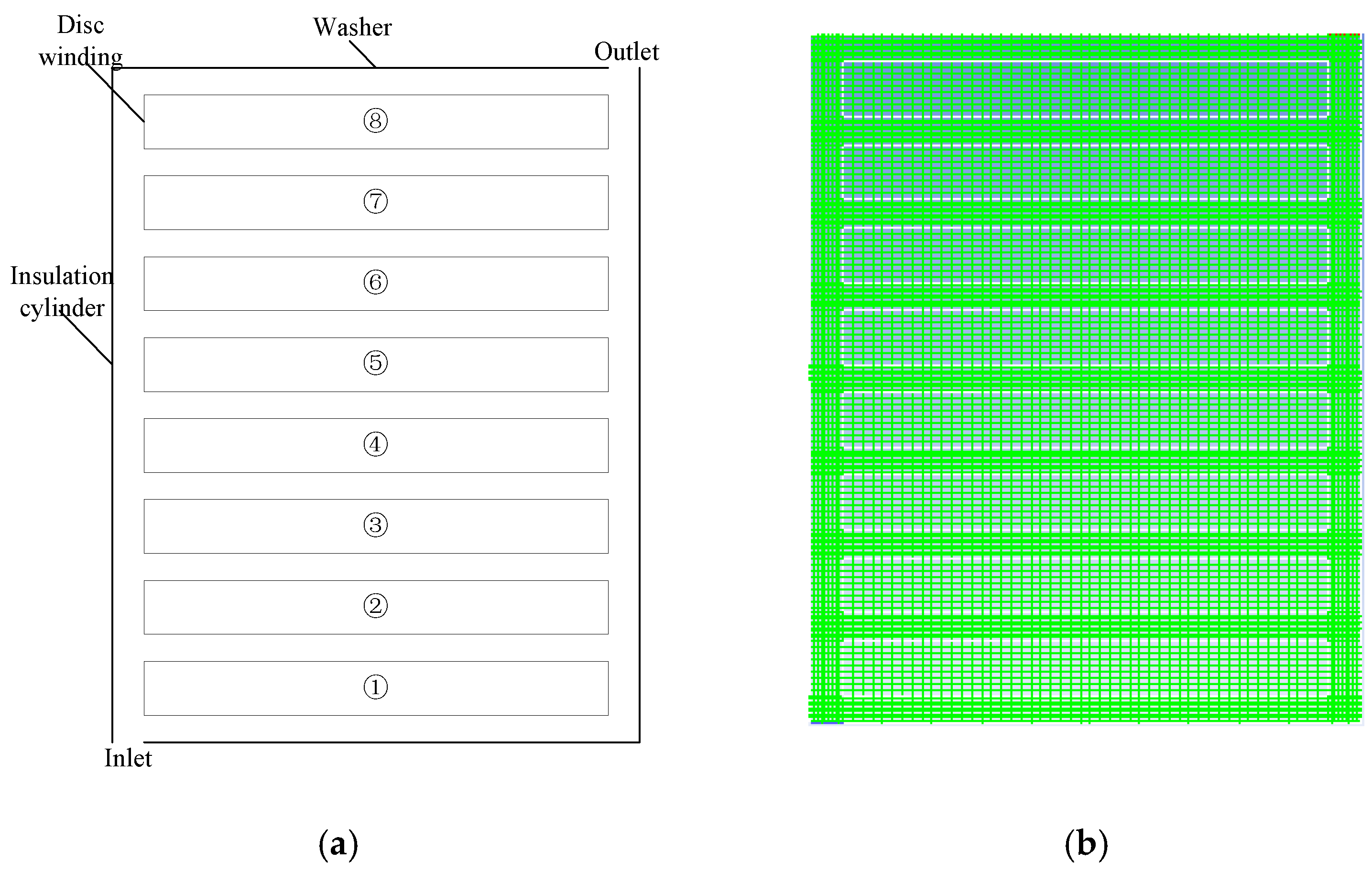
3.1. Transformer Winding Model

In order to verify the applicability and efficiency of the proposed algorithm for complex structures and multi-field coupling problems, a fluid-thermal field coupling problem of an oil-immersed transformer winding model is taken as instance and analyzed in this paper. A two-dimensional model of the transformer winding is selected and analyzed [42,43]. The sizes of this model are listed in

Table 1. Model Sizes.

Component	Size
Total Size of Model	0.1 m × 0.125 m
Size of Disc	0.088 m × 0.01 m
Length of Insulation Cylinder	0.125 m
Length of Washer	0.094 m
Width of Inlet	0.06 m
Width of Outlet	0.06 m

. The fluid area of the model consists of two vertical oil ducts and nine horizontal oil ducts. The geometric graph is shown in Figure 2a. When meshing the model, the grid of the oil ducts should be more elaborate than that of the discs, as shown in Figure 2b.

In the coupling field analysis, the physical parameters of the transformer oil are the linear or quadratic functions of the temperature [10], while others are deemed as constants, as listed in

Table 2. Physical parameters of model.

Materials	Physical Parameters	Function Fitting
Transformer oil	Density/kg·m−3	1098.72 − 0.712 T
	Specific heat capacity/J·(kg·K)−1	807.163 + 3.58 T
	Heat conductivity/W·(m·K)−1	0.1509 − 7.101 × 10−5 T
	Viscosity/Pa·s	0.0846 − 4 × 10−4T + 5 × 10−7 T2
Winding	Density/kg·m−3	8900
	Specific heat capacity/J·(kg·K)−1	381
	Heat conductivity/W·(m·K)−1	387.6

.

At the inlet, the boundary conditions u = 0, v = 0.05 m/s, and T = 330 K are applied. At the outlet, the pressure boundary conditions u = 0, p = 0, and $\partial T/\partial n=0$ are applied.

The no slip boundary, that is, u = 0, v = 0, and $\partial T/\partial n=0$, is applied on the washer and insulating cylinder. Their heat conductivities are very small and thus they are considered as adiabatic boundaries. The boundary of the disc is a fluid-solid coupling one.

As is known to all, the ohmic loss and eddy-current loss produced in the discs is the heat source for the whole model, while the ohmic loss accounts for the main part. The effect of the temperature on its resistance should be taken into account, and the winding loss should be adjusted considering the influence of the temperature when calculating the temperature field, which is defined in Reference [47]:

$$P=P_0\left(1+\beta \left(T-T_0\right)\right)$$

(26)

where P is the windings loss density per element area, P₀ is the winding loss density calculated at the initial temperature T₀. When the temperature is 273 K, the density of winding loss per element area is 2.27 × 10⁵ W/m². β represents the temperature coefficient of the metal conductors and the value of the copper is 0.00393 (1/K).

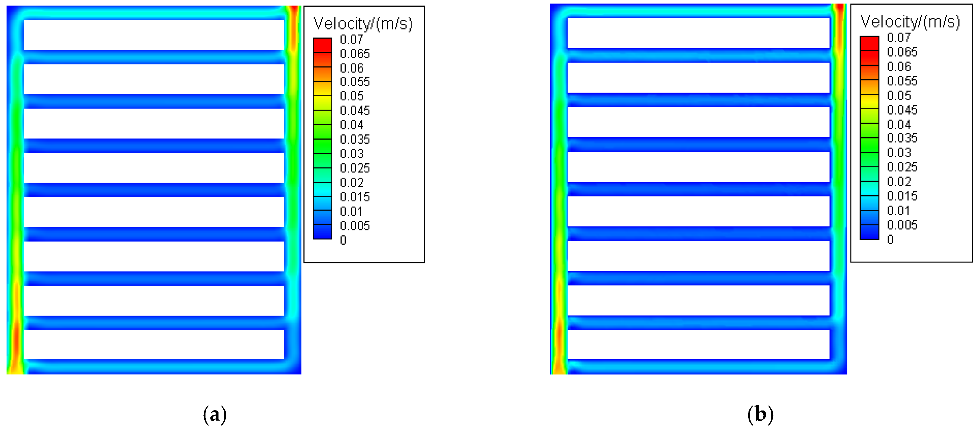
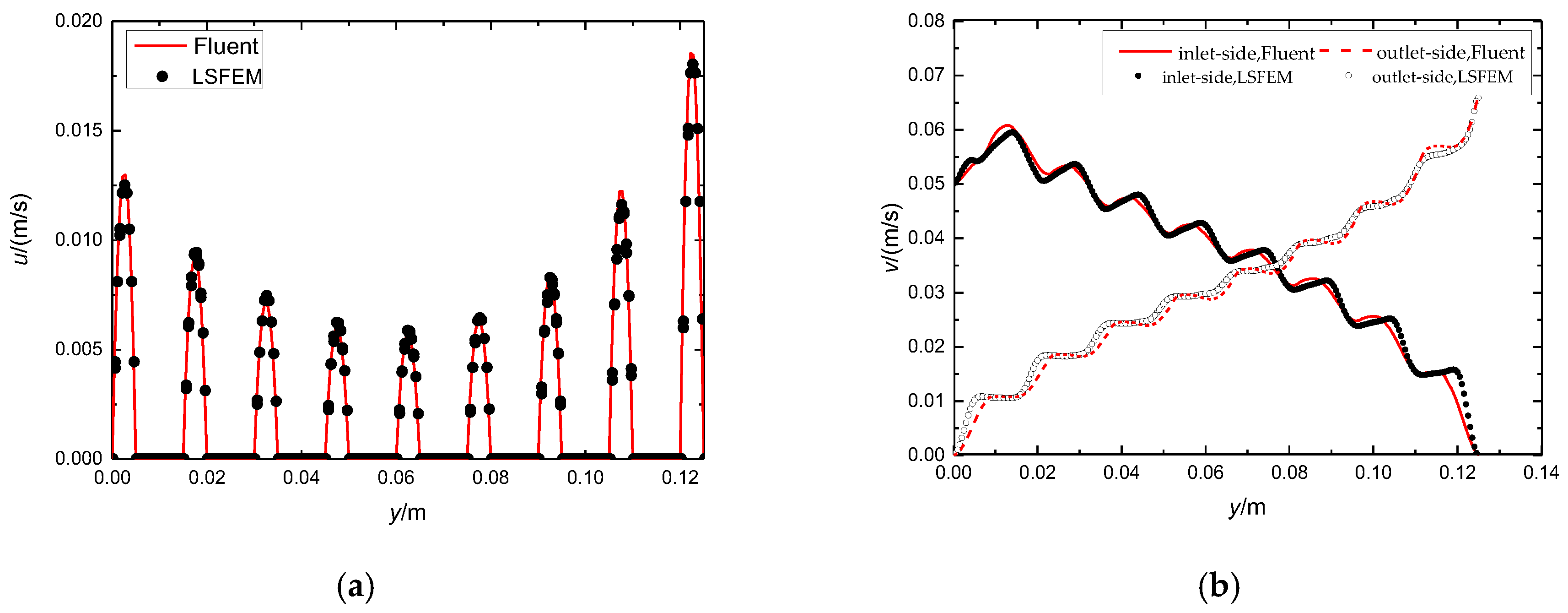
3.2. Velocity Distribution Analysis

The results by the conventional LSFEM [42,43] and the adopted dimensionless LSFEM are basically equal, the velocity distributions of the local winding model, calculated by the dimensionless LSFEM and Fluent software, are shown in Figure 3.

From Figure 3, we can see that the velocities at the horizontal and vertical oil ducts calculated by the proposed algorithm and Fluent software are almost the same, which is in accordance with the results computed by the conventional LSFEM and Fluent software [42]. In order to further illustrate the accuracy of the proposed algorithm, the velocity components of the two vertical oil ducts in different directions, x direction and y direction, are extracted, as is drawn in Figure 4.

In Figure 4a, from the bottom horizontal oil ducts to the top ones, the velocity of the horizontal oil decreases first and then increases. The velocity component of the x axis of the top horizontal oil duct is the largest, while the minimum velocity component of the x axis is in the middle oil duct. The velocity distributions are also in accord with results in Reference [42]. In Figure 4b, from the inlet to the top of the oil duct, the velocity of the vertical oil duct on the inlet side decreases in the form of fluctuations. The maximum velocity is at the place 0.015 m to the inlet. From the bottom of the oil duct to the outlet, the velocity of the vertical oil duct on the outlet side decreases in the form of fluctuations. The maximum velocity is at the outlet.

To sum up, the results of the dimensionless LSFEM are basically the same as those of Fluent software. In such a way, the accuracy of the dimensionless LSFEM scheme for the calculation of fluid field is proved.

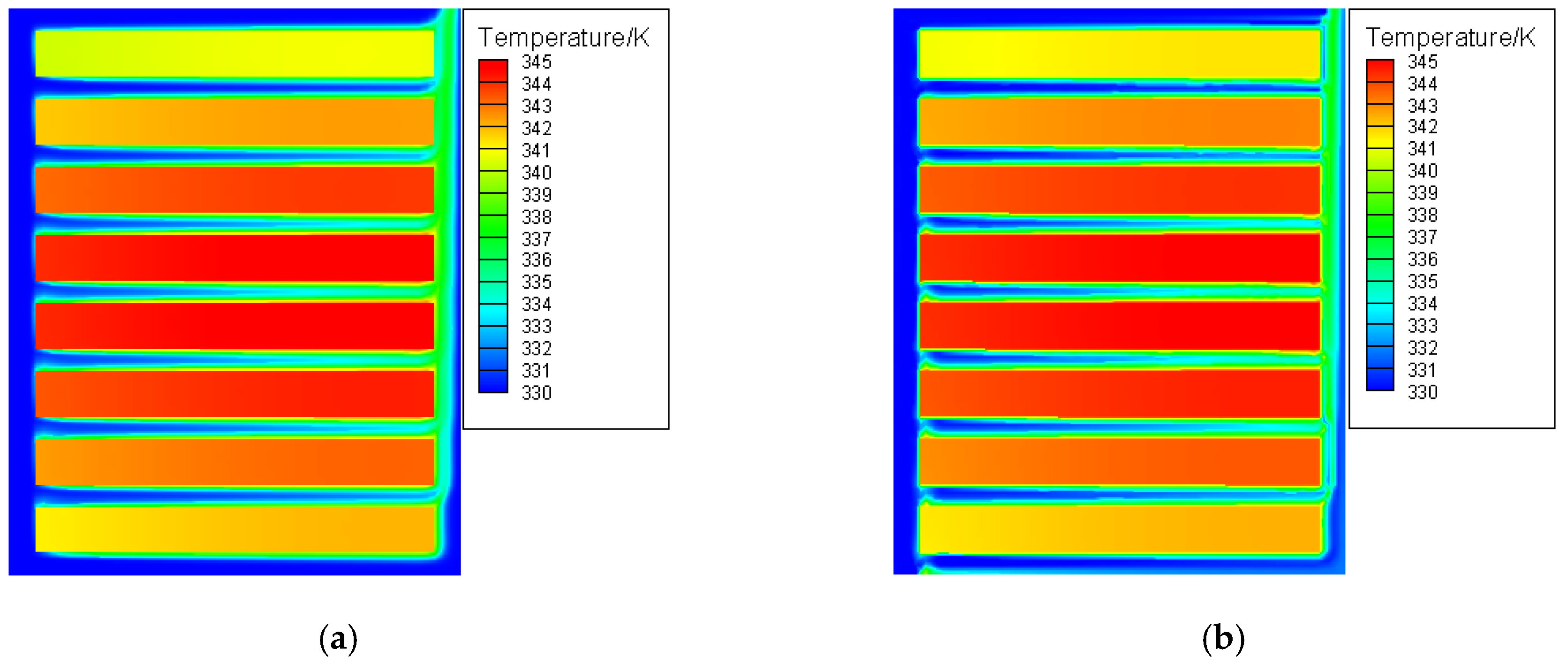
3.3. Temperature Distribution Analysis

The temperature distribution calculated by the proposed coupling algorithm and Fluent software are shown in Figure 5.

The temperature distributions are almost identical to the results in Reference [42], which are obtained by a combination of the conventional LSFEM and UFEM. For the sake of concise illustration, the discs are numbered in sequence, as shown in Figure 1a. In Figure 5, the temperatures of the discs increase first and then decrease in the order of one to eight. The temperature of the 8th disc is the lowest, while the temperatures of the fourth and fifth discs are the highest. The temperatures on the right-side of discs are higher than that on the left-side. The results obtained by the proposed algorithm are basically the same as those by the Fluent software.

The temperature values of the 1/4 vertical line on the left and right sides of the discs are extracted separately, as listed in

Table 3. Average temperature of discs calculated by Fluent and the UFEM (K).

Sequence Number of Disc	Left 1/4			Right 1/4
	UFEM	Fluent	Error	UFEM	Fluent	Error
1	341.5	340.9	+0.6	342.0	341.5	+0.5
2	342.8	342.1	+0.7	343.3	342.6	+0.7
3	343.7	343.1	+0.6	344.2	343.6	+0.6
4	344.2	343.7	+0.5	344.7	344.2	+0.5
5	344.3	343.7	+0.6	344.7	344.2	+0.5
6	343.5	343.0	+0.5	343.9	343.4	+0.5
7	342.3	341.7	+0.6	342.7	342.1	+0.6
8	340.9	340.3	+0.6	341.2	340.6	+0.6

.

As can be seen from Table 3, the highest temperature can be found on the right-side of the fourth disc and is 344.7 K, and the lowest temperature is on the left-side of the eight disc and is 340.9 K. The temperature difference is 3.8 K. The temperature of the right-side of the disc is 0.46 K higher than that of the left-side, on average.

Compared with the results obtained by Fluent software, the thermal field calculated by the proposed algorithm is slightly higher. The average temperature difference at the left 1/4 and the right 1/4 are 0.59 K and 0.56 K, respectively. The maximum difference is 0.7 K at the right 1/4 of the second disc, and its relative error is 0.2%.

The reasons for the difference of the results between the proposed method and Fluent software are concluded as follows:

(1)

Since the indirect coupling method proposed in this paper is a combination of the dimensionless LSFEM and UFEM, while Fluent software is based on FVM, the different principle of FEM and FVM could result in some deviations.

(2)

Different methods are adopted to deal with boundary conditions by FEM and FVM, which could bring some influence on the calculation results.

(3)

There are eight nodes per element for solving the fluid field by the LSFEM, while nine nodes per element to solve the thermal field by the UFEM, which adopts the second-order element. In contrast, Fluent software adopts the linear element. So their interpolation methods are different.

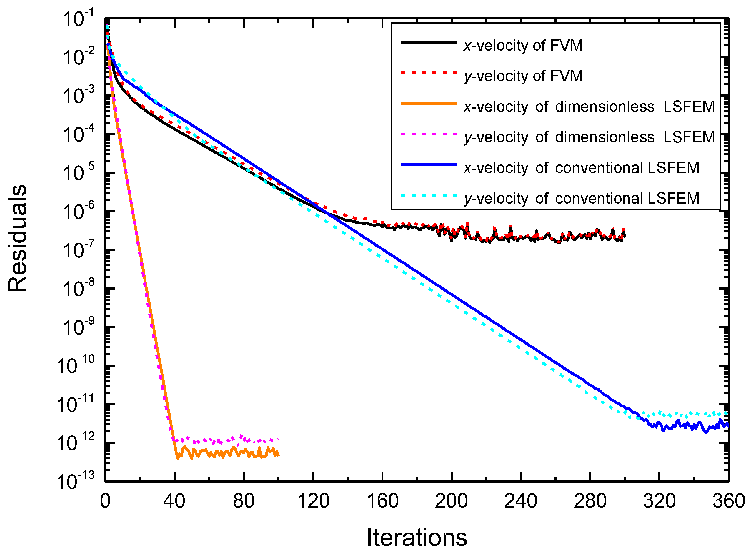
3.4. Convergence Analysis

While the above velocity and temperature distributions of the winding model, obtained by the Fluent software and the combination of conventional LSFEM and UFEM, respectively, are almost the same as those obtained by the proposed method in this paper, their convergence rates are different. The proposed method adopts the nondimensionalization of the Stokes equations and the preconditioning for the equation’s global stiffness matrix is conducted by the JPCGM and TSEM, so the corresponding equation converges faster. In order to illustrate the influence of the penalty function and different LSFEM schemes on the convergence rate, the iteration numbers, convergence time, and the condition numbers before and after preconditioning of the global stiffness matrix are listed in

Table 4. Convergence of discrete equations with different schemes and penalty functions.

Preconditioned Methods		JPCGM			JPCGM & TSEM
Penalty Function Size		104	106	108	108	108	108
Conventional Scheme	Condition Number 1	1.40 × 1018	1.40 × 1020	1.40 × 1022	1.88 × 1018	1.88 × 1020	1.88 × 1022
	Condition Number 2	9.89 × 109			1.13 × 108
	Iteration Numbers	Misconvergence			127	127	127
	Computation Time (s)				618	614	621
Dimensionless Scheme	Condition Number 1	8.27 × 1012	8.23 × 1014	8.23 × 1016	8.27 × 1012	8.23 × 1014	8.23 × 1016
	Condition Number 2	2.55 × 107			2.55 × 107
	Iteration Numbers	Convergence, wrong results			24	24	24
	Computation Time (s)				125	126	126

, where condition number one stands for the condition number before preconditioning and condition number two represents the condition number after preconditioning.

As can be seen from Table 4, the larger the value of a penalty function, the larger the condition number of the equations. However, all the three condition numbers of the conventional scheme can be reduced to 1.13 × 10⁸, and all the three condition numbers of the dimensionless scheme can be reduced to 2.55 × 10⁷ by JPCGM and TSEM. Therefore, even if the penalty function is different, the number of iterations and time for solving the equations is approximately the same after preconditioning by the JPCGM and TSEM.

For the two different LSFEM schemes, the condition number of the dimensionless scheme is smaller than that of the conventional scheme, and the number of iterations and the computation time of the dimensionless scheme is much smaller. It can be explained that the nondimensionalization process on the equations amounts to a preconditioning and the combination of nondimensionalization and JPCGM and TSEM can solve the fluid field more efficiently.

From Table 4 we can see that with the application of the JPCGM only, the conventional LSFEM scheme cannot get the convergent solution. Thus, the use of the dimensionless LSFEM, whose iteration number and computation time is meaningless, will obtain a wrong solution. The reason may be that the equations are seriously ill-conditioned in the neighborhood of zero. On the other hand, solutions with a good accuracy can be obtained for the two different LSFEMs by the combination of JPCGM and TSEM.

In addition, we can find that the two different LSFEMs based on the combination of JPCGM and TSEM converge effectively when the residual velocity is less than the convergence criterion, 1 × 10⁻⁶. However, for the Fluent software, it cannot continually converge when the velocity residuals reach the residual velocity. On the contrary, the convergence of the two different LSFEMs maintains the same speed and stays steady. In order to further analyze the minimum residual and convergence efficiency of the LSFEMs, the convergence criterion is defined as the velocity residuals less than 1 × 10⁻¹⁵, and the residual data are recorded. Figure 6 gives the convergence curves of the mentioned methods and shows that the two LSFEMs can get smaller convergence residuals than the Fluent software.

From Figure 6, we can see that the convergence trends of the velocity residuals in x and y directions are basically the same.

For the Fluent software based on FVM, the velocity residuals converge faster than that of the conventional LSFEM in the initial iteration stage; but the iteration rate decreases gradually. When the iteration reaches about 150 steps, the convergence is terminated. The minimum residual of convergence is larger than 1 × 10⁻⁷, and then the residuals oscillate between 1 × 10⁻⁶ and 1 × 10⁻⁷.

The convergence rate of the conventional LSFEM is approximately equal to that of Fluent, but the iterative residual is smaller. When the iteration reaches about 300 steps, the residuals tend to be stable and oscillate between 1 × 10⁻¹¹ and 1 × 10⁻¹².

The dimensionless LSFEM scheme converges continuously at a high rate. When the iteration reaches about 40 steps, the convergence is terminated and then the residuals tend to be stable and oscillate between 1 × 10⁻¹² and 1 × 10⁻¹³. Some conclusions can be achieved as follows:

(1)

Among these three calculation methods, the convergence rate of the dimensionless LSFEM scheme is the fastest, followed by the Fluent software based on the FVM, and finally the conventional LSFEM. In fact, the convergence rates of the latter two methods are very close.

(2)

During the convergence process, the residuals of dimensionless and conventional LSFEM schemes are much smaller than those of the Fluent software. The smallest residuals can be obtained by the dimensionless LSFEM scheme while the residuals of the Fluent software are the largest.

To sum up, the LSFEM has a better convergence and lower residual than the Fluent software.

4. Conclusions

In this paper, an efficient indirect coupling algorithm is adopted to analyze fluid-thermal coupling problems. Two different LSFEM schemes are analyzed and compared with Fluent software. Conclusions are drawn as follows:

(1)

Taking the results obtained by Fluent as a reference, the relative error of outlet velocity of the local winding computed by LSFEM is about 0.4%. The temperature difference between the upwind FEM and Fluent is less than 0.7 K. The LSFEM is stable and the numerical oscillations can be avoided without adding additional upwind schemes.

(2)

The combination of JPCGM and TSEM can effectively reduce the condition number of the equations and handle the ill-conditioned problems of the stiffness matrix. The larger the penalty functions, the larger the condition number of equations. It should be pointed out that the condition number can be reduced to the same value by preconditioning.

(3)

Compared with the FVM, the algorithm obtained by the dimensionless LSFEM scheme has better robustness, faster convergence, and lower residuals.

References

1. Heathcote, M.J. The J & P Transformer Book; Johnson & Phillips Ltd.: Karachi, Pakistan, 2007; pp. 121–187. [Google Scholar]
2. Higaki, M.; Kako, Y.; Moriyama, M.; Hirano, M.; Hiraishi, K.; Kurita, K. Static electrification and partial discharges caused by oil flow in forced oil cooled core type transformers. IEEE Trans. Power Appar. Syst. 1979, 98, 1259–1267. [Google Scholar] [CrossRef]
3. Wang, X.C.; Tao, J.P. Temperature field research of large forced-directed oil cooling transformer. Transformer 2008, 7, 6–10. [Google Scholar]
4. Sen, P.K.; Pansuwan, S. Overloading and loss-of-life assessment guidelines of oil-cooled transformers. In Proceedings of the 2001 Rural Electric Power Conference, Little Rock, AR, USA, 29 April–1 May 2001; pp. B4/1–B4/8. [Google Scholar]
5. Sefidgaran, M.; Mirzaie, M.; Ebrahimzadeh, A. Reliability model of the power transformer with ONAF cooling. Int. J. Electr. Power Energy Syst. 2011, 35, 97–104. [Google Scholar] [CrossRef]
6. Krause, C. Power Transformer insulation-history, technology and design. IEEE Trans. Dielectr. Electr. Insul. 2012, 19, 1941–1947. [Google Scholar] [CrossRef]
7. Raeisian, L.; Niazmand, H.; Ebrahimnia-Bajestan, E.; Werle, P. Thermal management of a distribution transformer: an optimization study of the cooling system using CFD and response surface methodology. Int. J. Electr. Power Energy Syst. 2018, 104, 443–455. [Google Scholar] [CrossRef]
8. IEEE. IEEE Guide for Loading Mineral-Oil-Immersed Transformers; IEEE: New York, NY, USA, 1996. [Google Scholar]
9. Perez, J. Fundamental principles of transformer thermal loading and protection. In Proceedings of the 11th IET International Conference on Developments in Power Systems Protection, Birmingham, UK, 29 March–1 April 2012; pp. 1–6. [Google Scholar]
10. Torriano, F.; Chaaban, M.; Picher, P. Numerical study of parameters affecting the temperature distribution in a disc-type transformer winding. Appl. Therm. Eng. 2010, 30, 2034–2044. [Google Scholar] [CrossRef]
11. Gong, R.H.; Ruan, J.J.; Chen, J.Z.; Quan, Y.; Wang, J. Analysis and experiment of hot-spot temperature rise of 110 kV three-phase three-limb transformer. Energies 2017, 10, 1079. [Google Scholar] [CrossRef]
12. Kranenborg, E.J.; Olsson, C.O.; Samuelsson, B.R.; Lundin, L.Å.; Missing, R.M. Numerical study on mixed convection and thermal streaking in power transformer windings. In Proceedings of the 5th European Thermal-Sciences Conference, Eindhoven, The Netherlands, 18–22 May 2008. [Google Scholar]
13. Skillen, A.; Revell, A.; Iacovides, H.; Wu, W. Numerical prediction of local hot-spot phenomena in transformer windings. Appl. Therm. Eng. 2012, 36, 96–105. [Google Scholar] [CrossRef]
14. Bengang, W.; Hua, H.; Junshang, L.; Nannan, W.; Mingqiu, D.; Tianyi, J. Three dimensional simulation technology research of split type cooling transformer based on finite volume method. Energy Procedia 2017, 141, 405–410. [Google Scholar] [CrossRef]
15. Chen, W.; Su, X.; Sun, C.; Pan, C.; Tang, J. Temperature distribution calculation based on FVM for oil-immersed power transformer windings. Electr. Power Autom. Equip. 2011, 31, 23–27. [Google Scholar]
16. Guo, R.; Lou, J.; Wang, Z.; Huang, H.; Wei, B.; Zhang, Y. Simulation and analysis of temperature field of the discrete cooling system transformer based on FLUENT. In Proceedings of the 2017 1st International Conference on Electrical Materials and Power Equipment, Xi’an, China, 14–17 May 2017; pp. 287–291. [Google Scholar]
17. Tsili, M.A.; Amoiralis, E.I.; Kladas, A.G.; Souflaris, A.T. Power transformer thermal analysis by using an advanced coupled 3D heat transfer and fluid flow FEM model. Int. J. Therm. Sci. 2012, 53, 188–201. [Google Scholar] [CrossRef]
18. Li, L.; Niu, S.; Ho, S.L.; Fu, W.N.; Li, Y. A novel approach to investigate the hot-spot temperature rise in power transformers. IEEE Trans. Magn. 2015, 51, 1–4. [Google Scholar]
19. Amoiralis, E.I.; Tsili, M.A.; Kladas, A.G.; Souflaris, A.T. Geometry optimization of power transformer cooling system based on coupled 3D FEM thermal-CFD analysis. In Proceedings of the 2010 14th Biennial IEEE Conference on Electromagnetic Field Computation, Chicago, IL, USA, 9–12 May 2010. [Google Scholar]
20. Torriano, F.; Campelo, H.; Quintela, M.; Labbé, P.; Picher, P. Numerical and experimental thermofluid investigation of different disc-type power transformer winding arrangements. Int. J. Heat Fluid Flow. 2018, 69, 62–72. [Google Scholar] [CrossRef]
21. Córdoba, P.A.; Silin, N.; Osorio, D.; Dari, E. An experimental study of natural convection in a distribution transformer slice model. Int. J. Therm. Sci. 2018, 129, 94–105. [Google Scholar] [CrossRef]
22. Arabul, A.Y.; Arabul, F.K.; Senol, I. Experimental thermal investigation of an ONAN distribution transformer by fiber optic sensors. Electr. Power Syst. Res. 2018, 155, 320–330. [Google Scholar] [CrossRef]
23. Zhang, X.; Daghrah, M.; Wang, Z.; Liu, Q.; Jarman, P.; Negro, M. Experimental verification of dimensional analysis results on flow distribution and pressure drop for disc-type windings in od cooling modes. IEEE Trans. Power Deliv. 2018, 33, 1647–1656. [Google Scholar] [CrossRef]
24. Godina, R.; Rodrigues, E.M.G.; Matias, J.C.O.; Catalão, J.P.S. Effect of loads and other key factors on oil-transformer ageing: Sustainability benefits and challenges. Energies 2015, 8, 12147–12186. [Google Scholar] [CrossRef]
25. Ramos, J.C.; Beiza, M.; Gastelurrutia, J.; Rivas, A.; Antón, R.; Larraona, G.S. Numerical modelling of the natural ventilation of underground transformer substations. Appl. Therm. Eng. 2013, 51, 852–863. [Google Scholar] [CrossRef]
26. Wang, L.; Zhou, L.; Tang, H.; Wang, D.; Cui, Y. Numerical and experimental validation of variation of power transformers’ thermal time constants with load factor. Appl. Therm. Eng. 2017, 126, 939–948. [Google Scholar] [CrossRef]
27. Zhang, Y.; Ho, S.L.; Fu, W. Applying response surface method to oil-immersed transformer cooling system for design optimization. IEEE Trans. Magn. 2018, 1–5. [Google Scholar] [CrossRef]
28. Liao, C.; Ruan, J.; Liu, C.; Wen, W.; Du, Z. 3-D coupled electromagnetic-fluid-thermal analysis of oil-immersed triangular wound core transformer. IEEE Trans. Magn. 2014, 50, 1–4. [Google Scholar] [CrossRef]
29. Wang, Q.; Wang, H.; Peng, Z.; Liu, P.; Zhang, T.; Hu, W. 3-D coupled electromagnetic-fluid-thermal analysis of epoxy impregnated paper converter transformer bushings. IEEE Trans. Dielectr. Electr. Insul. 2017, 24, 630–638. [Google Scholar] [CrossRef]
30. Liu, Y.; Li, G.; Guan, L.; Li, Z. The single-active-part structure of the UHVDC converter transformer with the UHVAC power grid. CSEE J. Power Energy Syst. 2017, 3, 243–252. [Google Scholar] [CrossRef]
31. Zhang, B.Z.; Yin, J.A.; Zhang, H.J. Numerical method of fluid mechanics. Mech. Eng. Press. 2003, 68–180. [Google Scholar]
32. Hendriana, D.; Bathe, K. On upwind methods for parabolic finite elements in incompressible flows. Int. J. Numer. Methods Eng. 2015, 47, 317–340. [Google Scholar] [CrossRef]
33. Zienkiewicz, O.C.; Taylor, R.L.; Nithiarasu, P. The Finite Element Method for Fluid Dynamics, 6th ed.; Elsevier Butterworth-Heinemann: Oxford, UK, 2005; pp. 525–537. [Google Scholar]
34. Brooks, A.N.; Hughes, T.J.R. Streamline upwind/petrov-galerkin formulations for convection dominated flows with particular emphasis on the incompressible navier-stokes equations. Comput. Methods Appl. Mech. Eng. 2015, 32, 199–259. [Google Scholar] [CrossRef]
35. Heinrich, J.C.; Huyakorn, P.S.; Zienkiewicz, O.C.; Mitchell, A.R. An ‘upwind’ finite element scheme for two-dimensional convective transport equation. Int. J. Numer. Methods Eng. 2010, 11, 131–143. [Google Scholar] [CrossRef]
36. Liu, G.; Jin, Y.J.; Ma, Y.Q.; Wang, L.P.; Chi, C.; Li, L. Two-dimensional temperature field analysis of oil-immersed transformer based on non-uniformly heat source. High Volt. Eng. 2017, 43, 3361–3370. [Google Scholar]
37. Wang, Y.Q.; Ma, L.; Lü, F.C.; Bi, J.G.; Wang, L.; Wan, T. Calculation of 3D temperature field of oil immersed transformer by the combination of the finite element and finite volume method. High Volt. Eng. 2014, 40, 3179–3185. [Google Scholar]
38. Jiang, B.N. The least-squares finite element method. Int. J. Numer. Methods Eng. 1998, 54, 3591–3610. [Google Scholar]
39. Bochev, P.B.; Gunzburger, M.D. Least-Squares Finite Element Methods; Springer: Berlin, Germany, 2009; pp. S23–S24. [Google Scholar]
40. Pontaza, J.P. A least-squares finite element formulation for unsteady incompressible flows with improved velocity–pressure coupling. J. Comput. Phys. 2006, 217, 563–588. [Google Scholar] [CrossRef]
41. Tao, S.; Yang, Z.; Jiang, B.; Gu, W.J. Application comparison of least square finite element method and finite volume method in CFD. Comput. Aided Eng. 2012, 21, 1–6. [Google Scholar]
42. Xie, Y.Q.; Li, L.; Song, Y.W.; Wang, S.B. Multi-physical field coupled method for temperature rise of winding in oil-immersed power transformer. Proc. CSEE 2016, 36, 5957–5965. [Google Scholar]
43. Xie, Y.Q. Study on flow field and temperature field coupling finite element methods in oil-immersed power transformer. Ph.D. Thesis, North China Electric Power University (Beijing), Beijing, China, July 2017. [Google Scholar]
44. Fialko, S.Y.; Zeglen, F. Preconditioned conjugate gradient method for solution of large finite element problems on CPU and GPU. J. Telecommun. Inform. Technol. 2016, 2, 26–33. [Google Scholar]
45. Wallot, J. XLIX. Dimensional analysis. Lond. Edinb. Dublin Philos. Mag. J. Sci. 2009, 3, 496. [Google Scholar] [CrossRef]
46. Liu, C.S. A two-side equilibration method to reduce the condition number of an ill-posed linear system. Comput. Model. Eng. Sci. 2013, 91, 17–42. [Google Scholar]
47. Liao, C.B.; Ruan, J.J.; Liu, C.; Wen, W.; Wang, S.S.; Liang, S.Y. Comprehensive analysis of 3-D electromagnetic-fluid-thermal fields of oil-immersed transformer. Electr. Power Autom. Equip. 2015, 35, 150–155. [Google Scholar]
Figure 1. Process of fluid-thermal coupling calculation.
Energies 11 02357 g001
Figure 2. (a) Geometric graph of local winding model; (b) local winding model after meshing.
Energies 11 02357 g002
Figure 3. Velocity distribution contour: (a) calculation result by Fluent; (b) Calculation result by dimensionless LSFEM.
Energies 11 02357 g003
Figure 4. (a) Velocity distribution of u along the vertical center line; (b) Velocity distribution of v along the vertical center line of the vertical oil ducts.
Energies 11 02357 g004
Figure 5. Temperature distribution contour: (a) calculation result by Fluent; (b) calculation result by the upwind finite element method.
Energies 11 02357 g005
Figure 6. Comparison of convergence curves.
Energies 11 02357 g006