Primary Frequency Controller with Prediction-Based Droop Coefficient for Wind-Storage Systems under Spot Market Rules


1
School of Electrical Engineering, Southeast University, Nanjing 210096, Jiangsu, China
2
School of Electrical Engineering and Computer Science, Queensland University of Technology, Brisbane, QLD 4000, Australia
3
Illinois Institute of Technology, Chicago, IL 60616, USA
*
Authors to whom correspondence should be addressed.
Energies 2018, 11(9), 2340; https://doi.org/10.3390/en11092340
Submission received: 26 July 2018
/
Revised: 15 August 2018
/
Accepted: 22 August 2018
/
Published: 5 September 2018
(This article belongs to the Special Issue Solar and Wind Energy Forecasting)
Abstract
:Increasing penetration levels of asynchronous wind turbine generators (WTG) reduce the ability of the power system to maintain adequate frequency responses. WTG with the installation of battery energy storage systems (BESS) as wind-storage systems (WSS), not only reduce the intermittency but also provide a frequency response. Meanwhile, many studies indicate that using the dynamic droop coefficient of WSS in primary frequency control (PFC) based on the prediction values, is an effective way to enable the performance of WSS similar to conventional synchronous generators. This paper proposes a PFC for WSS with a prediction-based droop coefficient (PDC) according to the re-bid process under real-time spot market rules. Specifically, WSS update the values of the reference power and droop coefficient discretely at every bidding interval using near-term wind power and frequency prediction, which enables WSS to be more dispatchable in the view of transmission system operators (TSOs). Also, the accurate prediction method in the proposed PDC-PFC achieves the optimal arrangement of power from WTG and BESS in PFC. Finally, promising simulation results for a hybrid power system show the efficacy of the proposed PDC-PFC for WSS under different operating conditions.
1. Introduction
The use of wind energy has grown rapidly in the past decade, as wind turbine generators (WTG) are fuel-free and emissions-free [1]. Dramatically different from conventional synchronous generators, WTG output relies significantly on random wind speed, and the rotor speed of dominant type WTG is decoupled from the system frequency with no inertial capability [2]. These factors limit the further penetration of WTG in the power system. Also, primary frequency control (PFC) for synchronous generators is inappropriate for WTG. Thus, WTG with PFC abilities have become a topic of interest in the WTG research field.
Initially, WTG had no PFC function, due to the maximum power point tracking (MPPT) operation. Authors such as [3,4,5] have proposed the concept of virtual inertia, in which kinetic energy stored in the spinning rotor of WTG is released depending on frequency deviations. However, the accessible kinetic energy is limited, and may lead to secondary frequency drops in some cases. On the other hand, the concept of de-loaded operation for WTG in PFC was proposed in [4,6,7,8,9,10], which preserves the generating margin by keeping the WTG in a de-loaded operational state. In detail, shifting the maximum power point to the right sub-optimal point by overspeed rotor control is often adopted in the de-loaded control [6,7]. Pitch angle control is another example of de-loaded operation when wind speed is high [8,9]. Meanwhile, coordinated overspeed rotor control and pitch angle control [4,10] enable WTG to perform better in PFC. For example, the authors in [4] propose a PFC strategy by controlling the generator torque and the pitch angle using the real-time reference values, but without exploring a way to obtain them. Although promising, the de-loaded operation of WTG results in the loss of green energy due to a sub-optimal operation point, and makes it difficult for WTG to avoid unexpected issues in the longer term unless some dramatic steps are taken in this direction.
Realizing these dangers, several grid operators have embarked on storage technologies. For example, large scale energy storage systems (ESS) are being installed in California and a similar proposal has been made by the Australian Energy Market Operator (AEMO) [11]. Meanwhile, ESS have been utilized in PFC for WTG in the research field, such as [12,13,14]. This research shows that generally, with the support of ESS, wind-storage systems (WSS) become more reliable in PFC, but the large capacity of ESS cannot be avoided as WTG operate on the maximum power point. Thus, to combine the advantages of both sides, de-loaded WTG operation with the assistance of ESS has become the typical way for WSS in load frequency control (LFC), as mentioned in [15,16]. Also, the authors in [17] suggested a PFC method using variable droop coefficients, which reduces the stress on WTG and battery energy storage systems (BESS), especially when wind speed is low. Similarly, variable droop coefficients were applied in [18,19,20] to enable WSS to undertake the proper frequency regulation responsibility according to their real-time capability. In particular, a dynamic schedule and control strategy for WSS in LFC is proposed in [21], and a simple wind power prediction method is used to improve the frequency regulation performance of WSS. The authors in [22] also mention that short-term forecasting is the key to supporting unit commitment and economic dispatch.
Currently, the best way to dispatch WSS in the PFC has not been agreed upon by transmission system operators (TSOs) worldwide. Whether WSS is dispatch-friendly from the perspective of TSOs has become a major issue, which can be addressed with two improvements.
On the one hand, a proper and accurate prediction method must be selected. In previous research, the models that have been popularly applied to wind power prediction can be classified into three categories: physical models, statistical models and hybrid models. Specifically, physical methods, such as numerical weather prediction (NWP), are appropriate for long-term predictions [23]. Statistical models, including linear models and non-linear models are trained using historical data and usually outperform NWP models in short-term forecasting. Linear models such as auto regressive (AR), autoregressive moving average (ARMA), and autoregressive integrated moving average (ARIMA) are most widely used in [24,25,26]. Those methods perform well especially in short-term predictions. Furthermore, artificial neutral network (ANN) as a kind of most popular non-linear method in wind power prediction is shown in [27,28,29]. Typically, the back propagation neural network (BPNN), as shown in [27], is used to approximate the time series method, but is highly reliant on experience. Similarly, [28] proposes a lower upper bound estimation (LUBE) method to overcome the instability of neural network because it gives more freedom and flexibility. Also, [29] develops a forecasting engine wavelet ANN with a stochastic search technique for training the forecasting engine, capturing highly non-linear patterns in the data. Lastly, hybrid models combine different prediction methods. For example, a hybrid multi-model methodology is developed in [30], which combines multiple different machine learning algorithms including ANN, support vector machine (SVM), gradient boosting machine, and random forest, is relevant for different time horizons in short-term predictions. As shown in [31], another hybrid model is proposed for very short-term wind power ensemble forecasting when NWP is unavailable. Additionally, Kalman filter (KF) as a post-processing method can be combined with prediction methods to improve the performance. Weather research and forecasting with KF are combined as a prediction system in [32] for short-term wind power prediction. In [33], KF is used to support an SVM to improve the accurate of short-term wind speed prediction.
On the other hand, from the perspective of TSOs, taking full advantage of the current electricity market rules is an effective way to make WTG more dispatchable, which prevents WTG with real-time variable droop coefficients. Therefore, to make WSS more dispatchable, a PFC with prediction-based droop coefficient (PDC) for a utility-scale WSS is proposed in this paper. Specifically, the possible WTG output power and the trend of frequency deviations are forecasted, then this evidence is used to update the equivalent droop coefficient () of WSS every short time intervals. Various signals such as historical frequency (), WTG output () data and real-time system frequency deviations (), wind speed () are considered to ensure the WSS provide power output () following continuously. Additionally, compared with the control strategy in [21], two improvements are highlighted in PDC-PFC. First of all, WSS are more easily dispatched by the TSO, as the droop coefficients of WSS stay constant in every bidding interval. Meanwhile, KF-AR is selected as an accurate and proper method to make wind power prediction because AR performs well when the weather conditions are stable, especially in very short-term prediction. Also, the state matrix and measurement matrix form of KF are easier to combine with AR. In addition, although AR reflects less characteristics of WTG historical data than ANN, with the support of BESS that drawback can be addressed.
2. Bidding and Operation Mechanism of WSS under Spot Market Rules
A typical hybrid power system includes thermal generators and WSS, physically connected to the grid and dispatched by the TSO. To guarantee the stability of the system, the TSO dispatches generators according to their bids of supply and supply reserve. Thus, PFC ability is one of the compulsory considerations when the TSO dispatches the renewables.
Generally, the spot market bidding mechanism is very similar in many countries, including Australia’s National Electricity Market. The responsibility of the bidding mechanism is to balance the electricity demand and supply by dispatching the generated power through the spot market [34]. In detail, the complete bidding mechanism includes the daily bid process, the re-bid process, and the default bid process [35]. The daily bid process is for both conventional generators and WTG submitting their bids day-ahead. The re-bid process allows generators to update their bids according to the real-time conditions, to match the supply and demand more instantaneously. Normally, generators are allowed to submit their re-bids up until approximately five minutes prior to the TSO without changing the offer price [35]. Authors have noticed that WTG are price-insensitive generators but suffer noticeable errors in the daily bids [36], which can be effectively reduced in the re-bid process. Additionally, the default bid process involves standing bids that apply when no daily bid has been made. In summary, the re-bid process reduces the prediction period effectively, benefiting the prediction accuracy.
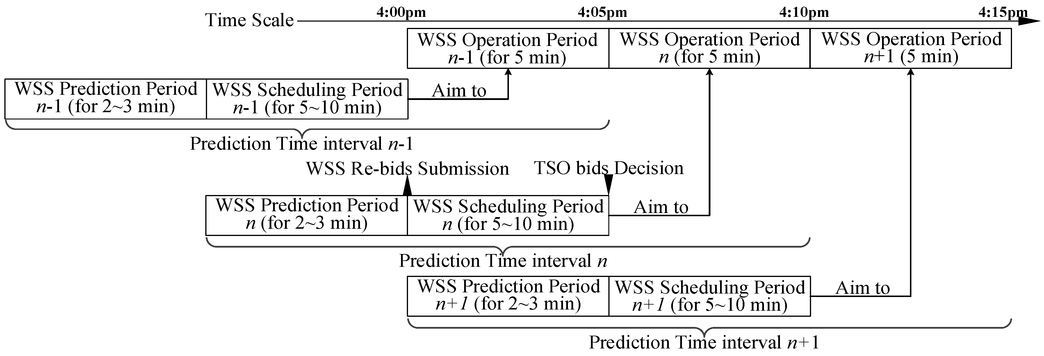
The operation loop of WSS in the re-bid process proposed in this paper is expressed in Figure 1. For example, WSS tend to be dispatched in the operational period between 4:05 p.m. and 4:10 p.m. WSS should submit their re-bids ( and ) 5~10 min earlier, and the TSO can re-schedule the generators’ bids in the market pool during the scheduling period and decide the generation combinations at 4:05 p.m. Before, WSS also spare 2~3 min as a prediction period to decide the re-bid submission. The time taken from the prediction period to the operation period is defined as the prediction time interval (PTI) and is typically 15 min.
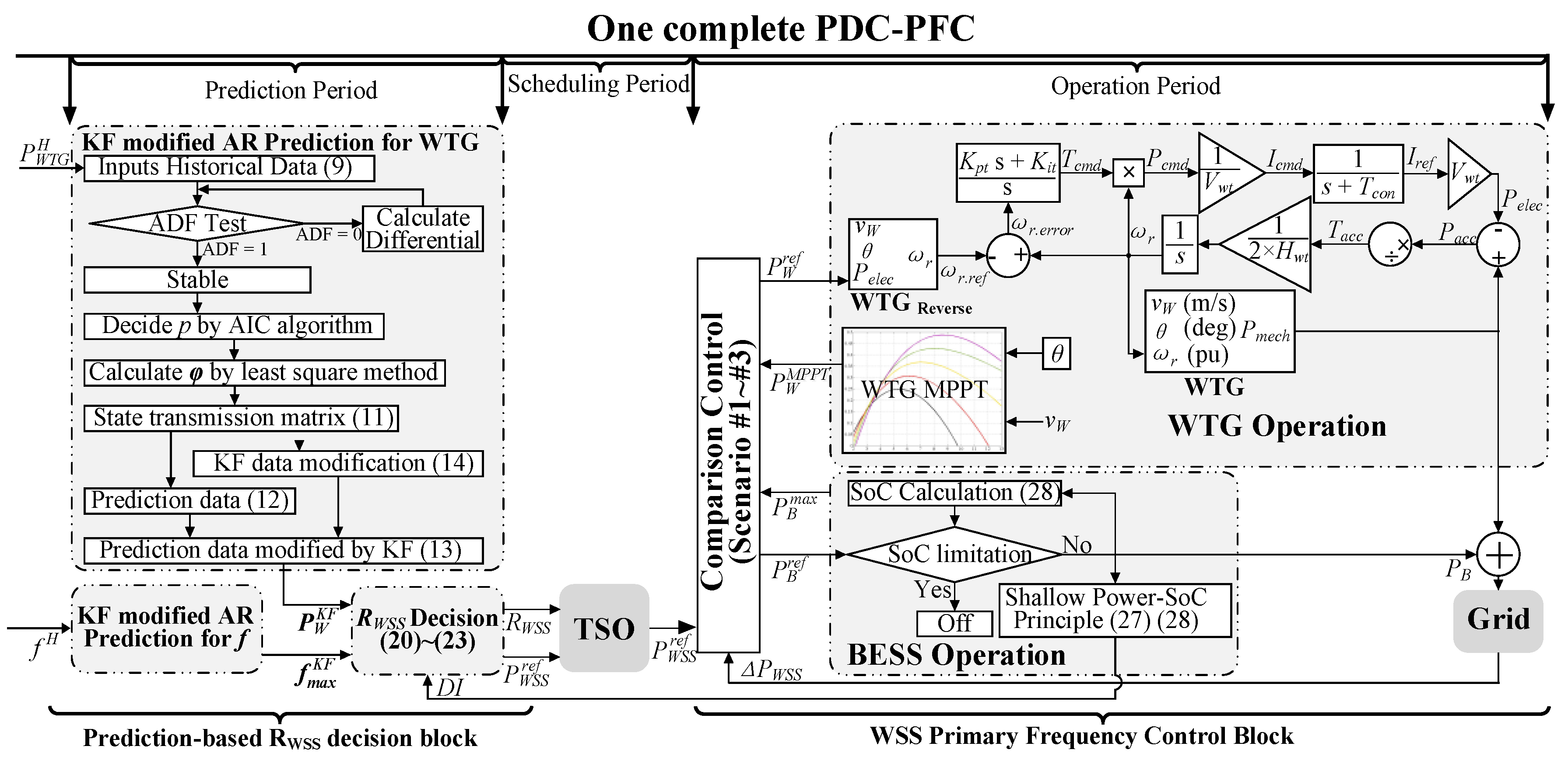
In the existing re-bid process, renewables are still regarded as generators with a lower degree of operation control. In other words, the re-bid process alone does not enable WSS to perform well in the PFC. Therefore, PDC-PFC, as seen in Figure 2 is proposed in this paper, by which WSS always aim at the preferable and in every bidding interval through the re-bid process, and provide corresponding , which is the sum of supply power () and supply reserve power ().
3. Primary Frequency Control with Prediction-Based Droop Coefficient for WSS
Dramatically different from conventional generators, is set by considering specific cases highly related to wind speed, instead of the inherent characteristics. PDC-PFC is utilized to determine the constant bidding power () and droop coefficient () of WSS for every bidding interval, which enables WSS to follow the market commitment and be more dispatchable.
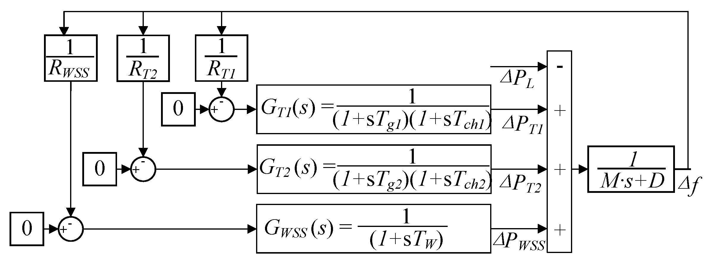
The dynamic model of a typical hybrid power system control area can be summarized as in Figure 3, in which the same type of generators are equivalent to one [37] with parameters as in Appendix A. Specifically, thermal generators contribute system inertia M with fixed droop coefficient , and WSS contribute no system inertia with decided by PDC-PFC. Variables in s domain have relationships as in Equations (1)–(5), and the transfer function of and is shown in Equation (6). Furthermore, the rate of change of the frequency (RoCoF), which is irrelevant to indicates the slope of the frequency drop at the beginning of the load disturbance as in Equation (7), and can finally increase the steady state of the frequency value, as in Equation (8). Thus, proper PFC from WSS can mitigate the frequency nadir, after load disturbances.
where, and are frequency response from WSS and thermal generators in PFC; and are the droop coefficients of WSS and thermal generators; represents the load disturbance and is the system frequency deviation; and are equivalent system inertia and damping; and are transfer functions of WSS and thermal generators; and are RoCoF and steady state of the frequency deviation after PFC.
Obviously, smaller is beneficial to the frequency stability, but WSS cannot guarantee enough reserved power in real time. PDC-PFC considers the uncertainty of WTG output, the limitation of the BESS capacity, and always decides the proper for every short-time interval.
Last, the complete PDC-PFC as shown in Figure 2, contains the “Prediction-based decision block” and “WSS primary frequency control block”. In detail, the “KF modified auto regressive (KF-AR) prediction” part is used to forecast the WTG output power and the trend in frequency deviation for the coming WSS operation period, and the decision” part decides the de-loaded level and the re-bid parameters for TSOs in KF modified auto regressive prediction. Meanwhile, in the WSS primary frequency control block, the “WTG operation” part and “BESS operation” part execute the control signals from the “Comparison control part” responding to the frequency regulation and wind speed fluctuations by absorbing and releasing power from the WTG and BESS. Generally, the inputs of PDC-PFC include historical frequency (), WTG output power (), real-time wind speed () from the WTG, frequency deviations (), and the output is , which is the sum of and consisting of and .
3.1. Prediction-Based Decision Block
The Prediction-based decision block consists of two parts, the Kalman filter modified auto regressive (KF-AR) prediction part and the decision part, which operate in sequence. According to the time-scale in Figure 1, PTI covers the “WSS prediction period”, “TSO scheduling period” and WSS operation period”, and a reasonable PTI is defined as 15 min.
3.1.1. KF-AR Prediction Part
Prediction of WTG output power is taken as an example to show the process of KF-AR Prediction, which has been fully summarized in Figure 2. First, historical WTG output power was collected as training data in Equation (9). The training data of WTG is from real-time recording and local memory without the process of data collection. Meanwhile, a 2~3 min prediction period was reserved for KF-AR prediction, as shown in Figure 1.
Furthermore, the AR model is a kind of a time-series analysis model that is regarded as a forecasting method for short-time intervals (such as 15 min in this paper). The boundary between AR, ARMA and ARIMA is not rigid, and the AR prediction process may use either of those methods. In detail, the historical values must pass the augmented Dickey–Fuller test (ADF = 1), because only stable data can be applied in the time-series analysis model. If fails to pass the ADF test (ADF = 0), a differential process is applied. As shown in Equation (10), p terms of historical data with coefficients are used. Specifically, the Akaike information criterion (AIC) and least square method are used to calculate p and respectively. However, AR prediction is normally with some forecast errors, which are further modified by KF as per Equations (11)–(16). In detail, p terms of compose the state transmission matrix F as in Equation (11), and the forecasted WTG output is calculated by Equation (12), which is similar to Equation (10). Last, is further modified to be by Equation (13) as the output.
where, is a matrix consisting of recorded WTG output power for the last prediction time interval; n represents the quantity of the historical data; is the state transmission matrix; is the forecasted value of without the KF modification; is the optimal value of WTG output by KF prediction; is used to link Equations (12) and (13); is with the measurement values based on forecasted wind speed; co-variances matrix of forecast error from to ; and are co-variances state estimation at and ; is the observation matrix (=1); represents Kalman gain; and are co-variance matrix of process noise and measurement noise, and both values are based on experience.
Similarly, the same prediction process is used for , which is another important parameter to calculate . As the frequency data is often recorded every 4 s in current power systems, historical frequency data () for the past several minutes is shown as Equation (18). Meanwhile, as PFC of WSS focuses more on the under-frequency situation, the maximum under frequency excursion () in every minute is chosen as per Equation (19). Finally, KF-AR prediction is applied to obtain for PTI.
where, is a matrix including 15 min frequency value, and each row represents a one-minute time interval; is a function used to calculate the minimum frequency values.
3.1.2. Decision Part
is determined by and in the decision part. Referring to conventional generators, the aim of WSS is 5% of supply power as a supply reserve power for PFC. However, the randomness of wind speed, is not a constant value. Thus, based on human understanding, when the fluctuation of the WTG output power is high, WSS should bid a smaller supply power with more reserved power for WSS in PFC and vice versa.
In detail, the standard deviation of indicates the fluctuation of WTG output, and the corresponding is calculated in Equation (20), which is further used to calculate proper as per Equation (21). Last, is obtained in Equation (22), and the state of the BESS is also involved. In this way, and keep updating every bidding interval, which enables WSS to be dispatched and to follow their commitment in PFC more easily.
where, is the de-loaded level of WTG, is the coefficient which shows the influences of WTG output power fluctuations on ; is the proposed re-bid power of WSS; is the reciprocal value of the droop coefficient; is the principle of ”shallow cycle operation profile” of batteries; is its threshold; shows the proportion of the moments that BESS operates on shallow cycle operation profile mode. Additionally, and are functions to calculate the standard deviation and the average values; is a counter. Positively, keeps constant within every WSS operation period in Figure 1. From the perspective of TSOs, WSS can be dispatched similar to a conventional generator in that particular period. Also, by considering the characteristics of WTG, varies every prediction time interval to remain optimized. Thus, WSS can always be regarded as conventional generators by PDC-PFC, and easier to dispatch.
In conclusion, the prediction-based decision block decides and of WSS for the next operation period through two processes. In particular, KF is applied to improve the accuracy of the prediction. Also, is a convincing value, because of the consideration of the states of WTG, BESS and system frequency deviations.
3.2. WSS Primary Frequency Control Block
Once and is confirmed by the TSO, the WSS Primary Frequency Control Block is applied to make sure the WSS ensures the reference power and respond to frequency deviation by adjusting the output of WTG () and BESS (). The complete WSS Primary Frequency Control Block is comprised of the “WTG operation” part, “BESS operation” part and “Comparison control” part, as already shown in Figure 2.
3.2.1. Comparison Control
Comparison control is the connection between the KF-based decision block and the WSS primary frequency control block. As shown in Figure 2, the demand signals ( and ) from the grid and available power ( and ) are compared to decide the and signals.
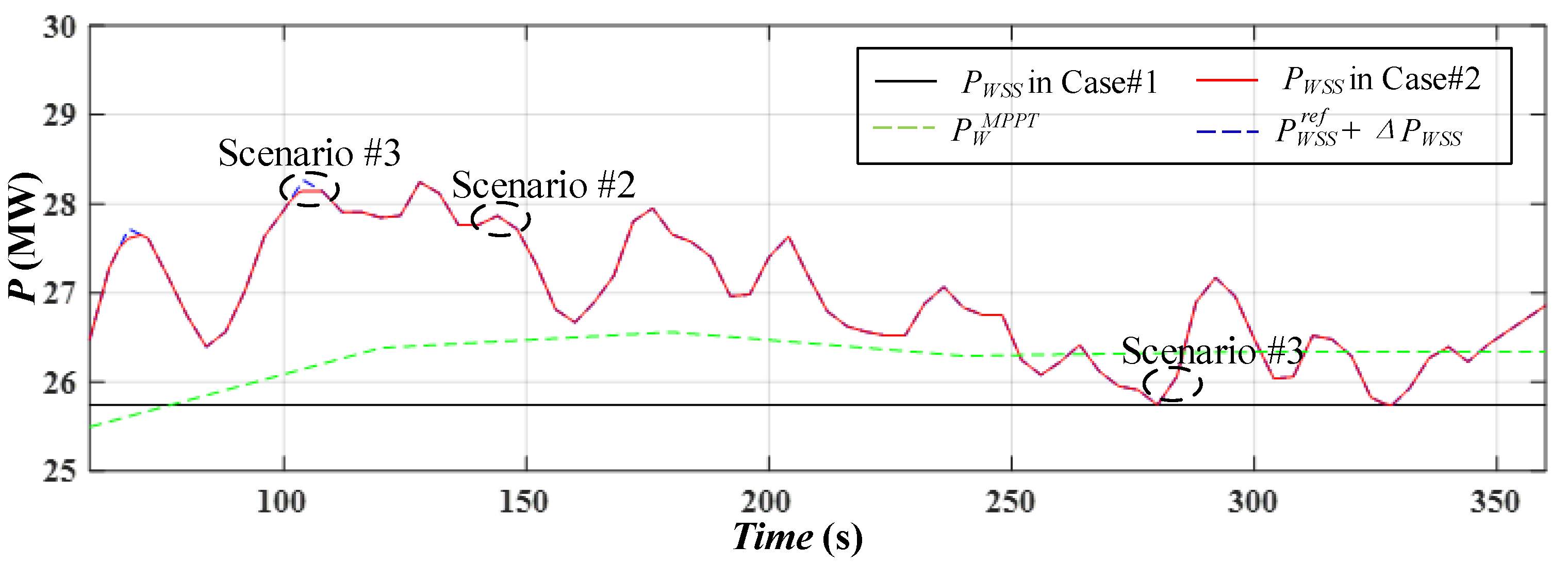
Taking the under-frequency situation as an example, three scenarios may happen in real-time operation. Details of the WTG and BESS energy management are shown in (24)–(26).
- Scenario #1: WTG with its reserved power supply the demand, if .
- Scenario #2: WTG with its reserved power and BESS supply the demand, if .
- Scenario #3: WTG with its reserved power and BESS supply all their power, but cannot meet the demand, if . The chance of Scenario #3 is extremely low in the proposed PDC-PFC, because of the dynamic and .
3.2.2. WTG Operation
MPPT is the basics of WTG operation, and the maximum output power of WTG is directly related to wind speed (). Moreover, DFIG as the dominant type of WTG, can operate on de-loaded mode, in which rotor speed can be accelerated up to 130% [1] to make WTG output power less than the maximum power point. Thus, WTG operation aims to achieve by releasing and absorbing power in a typical range, when the fluctuations of wind speed and frequency deviations happen. Particularly, the de-load level of WTG varied in real time, according to the predicted weather conditions and frequency performance in Equation (20), as a fixed de-load level results in either energy spilled or shortage. In addition, the dynamic model of WTG, including MPPT and de-loaded operation are shown in Figure 2, and the values of the parameters are listed in Appendix A. More details of the de-loaded operation block can be referred to in [21].
3.2.3. BESS Operation
Because of the randomness of wind speed, BESS are compulsory for dealing with unexpected issues to fulfil the bid commitment. As long as state of charge (SoC) of BESS is within the typical range, such as [0.2, 0.8], BESS respond to . Otherwise, BESS are switched off.
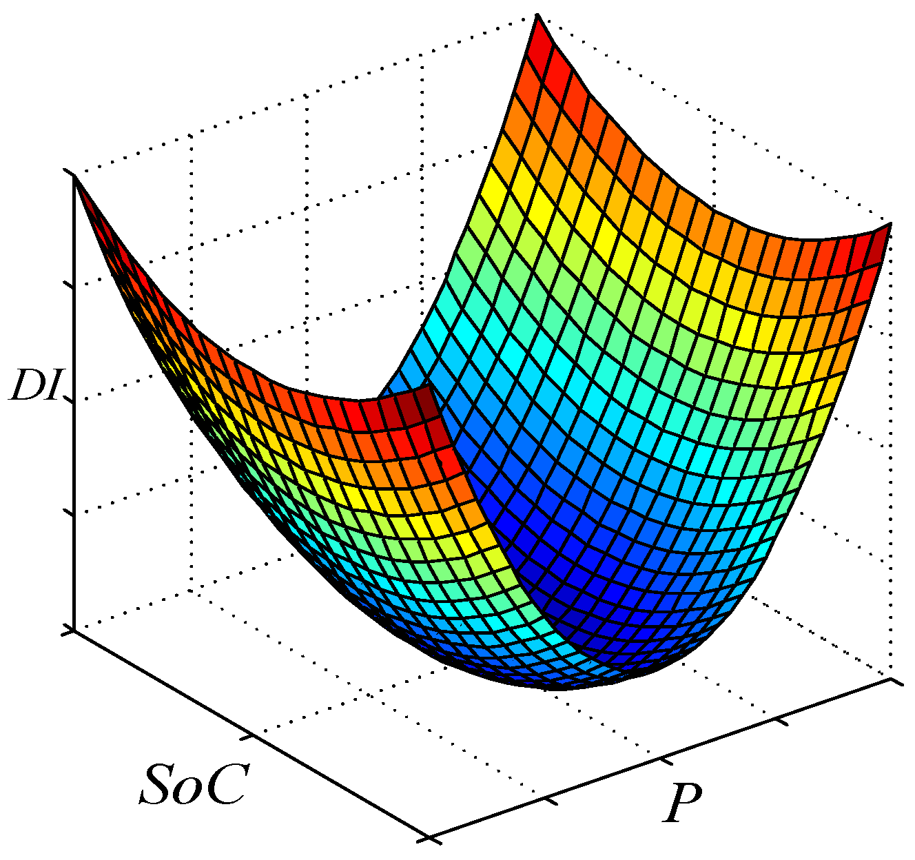
To extend BESS operation life and to avoid the occurrence of Scenario #3, the principle of shallow cycle operation profile for BESS is proposed in the BESS operation. The shallow cycle operation profile index is expressed in Equation (27), and SoC can be further expressed as a function of and in Equation (28).
where is the shallow cycle operation profile index at moment t; and are the charging and discharging power of BESS, and either and equals 0 at every t moment; is the state of charge of BESS at t moment; is the reference value; and are the charging and discharging efficiency of BESS, respectively.
Figure 4 is a more intuitive way to show the principle of shallow cycle operation profile. The light colored area represents the moment BESS belongs to the shallow cycle operation profile mode, and the warm colored area represents the opposite mode. The proportion of the moments of in the light colored area of all in the operation period affects the in Equation , which avoids the overuse of BESS.
In conclusion, PDC-PFC is achieved by the combination of KF-AR prediction and decision. In this way, WSS can perform very similarly to conventional generators in PFC. Specifically, and are carefully chosen in every bidding interval, and the power from WTG and BESS is well organized.
4. Simulation and Discussion
In the first part of this section, the performance of the proposed prediction-based decision block and WSS primary frequency control block are simulated. Also, the efficacy of the proposed PDC-PFC is investigated and compared with other conventional control strategies.
4.1. Performance of Prediction-Based Decision Block
The PTI in Figure 1 is assumed to be 15 min in the simulation by covering three periods of PDC-PFC. The values of and for the corresponding period is determined by (20)–(22), which in turn are based on the WTG output and from the past 15 min. Moreover, WTG often record their output power every minute in practice, n in equals 15 in (9), and m in also equals 15 in (18). The results of the predicted WTG output power and system frequency in PTI #1 is shown in Table 1 and Table 2, respectively. Other combinations of different wind speed situations and frequency excursions are created to represent typical time intervals and marked as PTI #2 and PTI #3, and the results are shown in Appendix B in Table A1, Table A2, Table A3 and Table A4.
Based on the process in Figure 2, the terms of AR model p of WTG and frequency excursion are both decided to be 10, according to the results of the ADF test and AIC algorithm. The least square method is applied to determine the coefficients of each term, and the transmission matrix F is obtained. The values of and are generated by KF-AR prediction, whereas and are calculated by AR prediction. Also, the KF-AR prediction values in PTI #1 (dotted black curve) are compared with the AR prediction values (dotted red curve) and the real values (dotted blue curve) in Figure 5a,b. Also, the errors between AR prediction, KF-AR prediction and the real values are listed in the third and fifth columns of Table 1, Table 2, and Table A1, Table A2, Table A3, Table A4. In the comparisons, values of are larger than in all those six tables. For example, in Table 1, of WTG output in PTI #1 equals 2.1605, while is 1.5680. In conclusion, KF-AR prediction values are very close to the real values, and much better than the AR prediction values, especially for the prediction of WTG output power.
Finally, according to the analysis of the prediction data listed in Table 1, Table 2, and Table A1, Table A2, Table A3, Table A4, the parameters of PDC-PFC in three PTI are shown in Table 3. Typically, as the average wind speed is medium with light fluctuations during PTI #1, the WTG has a 5.25% de-loaded value. By considering the possible maximum frequency excursion, the droop coefficient is set to be 22.34. Similarly, the WTG has a high de-loaded level of 19.49% because of heavy wind speed fluctuations during PTI #2. The corresponding droop coefficient is smaller at 14.45, which means that the WSS undertake less PFC responsibility, and avoid the unexpected issues. Also, during PTI #3, the WSS is under normal weather conditions, but the droop coefficient is set to be only 3.9 because of the large frequency excursion. To sum up, the WSS parameters chosen by PDC-PFC accord with human understanding, and the rationality of PDC-PFC has been partly proved.
4.2. Performance of WSS Primary Frequency Control Block
An open-loop control is used to simulate the performance of the WSS primary frequency control block, as shown in Figure 2. Taking PTI #1 as an example, the target power of WSS is the sum of MW and MW, and the available power is the sum of and MW. In particular, fluctuate in real-time in the same way as the values of in Table 1. Meanwhile, two cases as shown in Table 4, are used to verify the control block, by which the power output of WSS can achieve the target value. Additionally, BESS are assumed to be totally under the shallow P-SoC limitation before PTI #1, and is equal to 1 in this part.
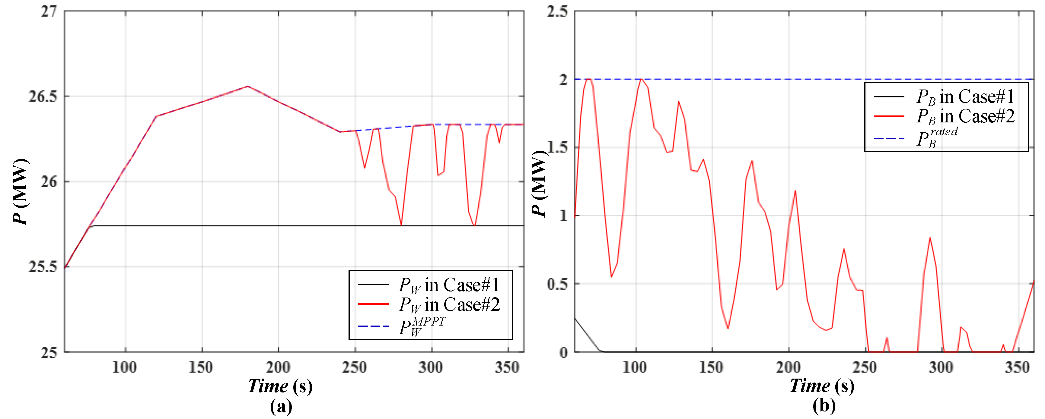
In Figure 6, the black and red lines representing the block can respond to the system demand and in those two cases, and the occurrences of the three scenarios are also marked. At the same time, WTG takes responsibility for the system demand for most of time, because the blue dotted line as the target value is nearly overlapped by the black (Case #1) and red (Case #2) lines. Moreover, the output power of WTG and BESS in Case #1 and Case #2 is compared with and as shown in Figure 7. Although is more than at the beginning of the interval, BESS compensate for the power shortage, and the system demand is still satisfied. In summary, PDC-PFC can manage the power of WTG and BESS to mitigate the fluctuations in WTG in Case #1 and respond to the system frequency deviations in Case #2.
4.3. Performance of PDC-PFC in Hybrid Power System
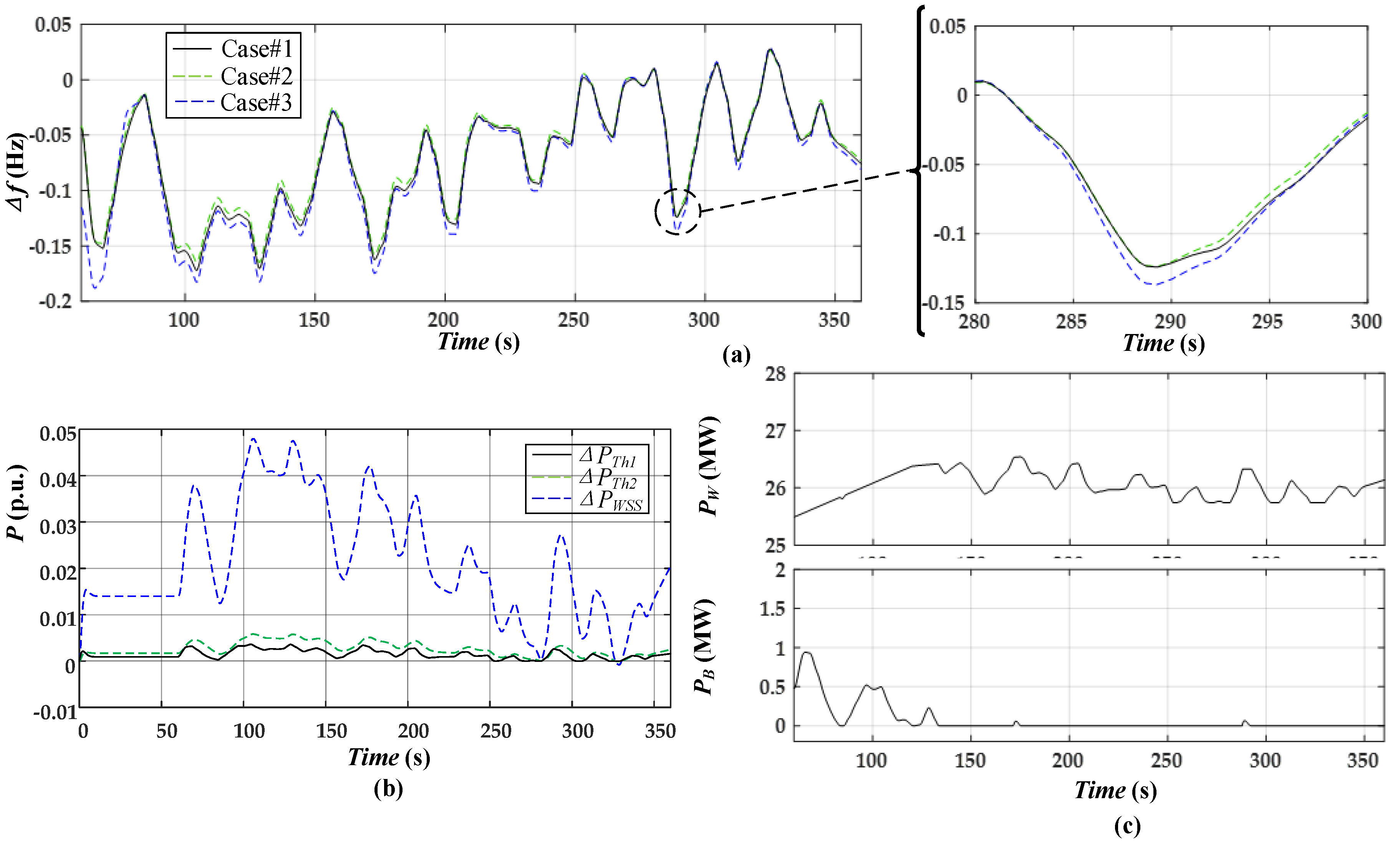
The performance of WSS equipped with PDC-PFC was simulated in the dynamic model of a hybrid power system, as in Figure 3 with parameters in Appendix A, and PDC-PFC was compared with two other cases (listed in Table 5). Specifically, the bidding power of two thermal generators , were 200 MW, 50 MW, and WSS 25.74 MW in PTI #1, feeding 250 MW demand.
The control performance in those three cases with the same fluctuations and load deviations are shown in Figure 8. Specifically, the frequency deviations in those three cases are shown in Figure 8a, the contribution of each generator including WSS is shown in Figure 8b, and the output power of WTG and BESS are shown in Figure 8c. Moreover, as the penetration of WTG replaces equivalent conventional generator and reduces the effective inertia of the system, Case #3 (blue dotted curve) has a lower frequency nadir in PFC than Case #2 (green dotted curve). However, the proposed WSS utilizes its droop coefficient combined with the fast response speed of WTG and BESS increases the frequency nadir in PFC in Case #1 (black curve). In conclusion, the proposed PDC-PFC in Case #1 demonstrated the best control performance, and WSS have a similar response as that of conventional coal-based synchronous generators.
4.4. Advantages of the Application of PDC-PFC
Further analysis of PDC-PFC is included in this part, and PDC-PFC is compared with several fixed de-loaded droop coefficients using AR prediction, as shown in Table 6. Also, three operation periods PTI #1–PTI #3 based on the values from Table 1, Table 2, and Table A1, Table A2, Table A3, Table A4 are used to show the adaptability and advantages of PDC-PFC. The following results show PDC-PFC enables WSS to operate similarly to conventional generators with proper combination of and , by considering real wind speed fluctuations and load deviations.
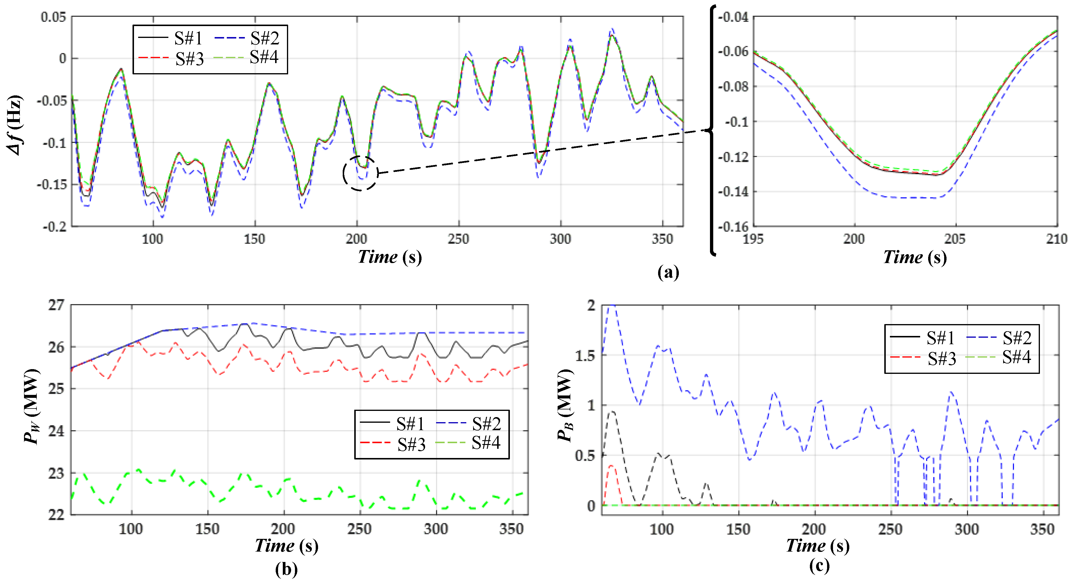
The performance of each strategy shown in Table 6 was evaluated in terms of frequency response with the utilization of WTG and BESS. As the details show in Figure 9a, S#2 (dotted blue curve) worsens the WSS performance in the frequency response because WSS bid the largest by replacing the equivalent amount of synchronous inertia, leaving the hybrid power system with the least inertia and WTG reserve with insufficient power for PFC. Meanwhile, WTG and BESS operate on and for most of the operation period, as shown in Figure 9b,c. Although the wind energy is fully utilized, a large part of the BESS capacity is also required with a bad shallow cycle operation profile index, which affects the sustainable use of BESS.
On the contrary, S#4 (dotted green curve) hash the highest de-loaded level, which leads to the lowest wind energy penetration as the smallest . It is clear the frequency performance (green curve) is satisfactory, as shown in Figure 9a, similar to S#2 and S#3. However, the highest de-loaded level with an inappropriate value of leads to a huge amount of wind energy spillage and abandonment to the use of BESS as in Figure 9b,c. Finally, S#3 (dotted red curve) is a relatively better choice than S#2 and S#4 for WSS in PTI #1, and S#1 (black curve) is the best choice on the basis of more accurate prediction data.
Furthermore, to highlight the efficacy of PDC-PFC and its ability to always find the proper combination of and , two more PTI were examined, and the results are summarized in Table 7. The results of Figure 9 are further verified by the concrete data of wind energy spillage and BESS capacity requirement in PTI #1. Also, it is obvious in PTI #2, PDC-PFC makes WTG with the largest de-loaded level, as wind speed fluctuates violently. The frequency performance of S#1 is much better than S#2 and S#3 and also better than S#4. Although, S#1 suffers the largest amount of wind energy spillage, less BESS capacity is required. Similarly, S#1 has the best control performance according to our comprehensive assessments, and balances the spilled wind energy and BESS capacity requirement. In conclusion, PDC-PFC can always decide the most suitable value of and for every short time interval according to the real-time conditions by using accurate prediction method. Also, PDC-PFC enables WSS to perform similarly to synchronous generators by dispatching WTG and BESS wisely.
5. Conclusions
If future power systems with high levels of renewables are to maintain acceptable levels of frequency response, all new and existing generators should be asked to contribute to the system frequency response. The participation of WTG in frequency response, especially in under-frequency situations is very necessary to ensure system stability. In this paper, PDC-PFC ensures that the performance of WSS is similar to conventional generators in a short time frame, which makes WSS more dispatchable from the perspective of TSOs.
Here, two innovations were considered in PDC-PFC. On the one hand, the spot market rule has been fully considered in PDC-PFC, and thus, from the perspective of TSOs, WSS can be regarded as conventional generators and are easier to dispatch. In detail, WSS joins the re-bid process of the spot market with constant and by the prediction-based decision block. Meanwhile, as and varies every re-bid interval according to real-time wind speed fluctuations and load deviations, WSS can always operate on the optimal operational conditions.
On the other hand, an accurate and proper method, KF-AR was used to improve the wind power prediction. Although AR reflects less characteristics of WTG historical data than ANN, the involvement of BESS can overcome that drawback. Moreover, AR has stable performance for the short-term prediction without the aid of experience, and KF further improves the prediction accuracy level.
In summary, with the application of AR-KF in PDC-PFC, WSS can satisfy the system frequency requirement, avoiding wind energy spillage and the excessive use of BESS in the current spot market rules. The simulation results show that WSS can guarantee smooth output power and the frequency response in every PTI under the control of PDC-PFC.
Author Contributions
Writing-Original Draft Preparation, S.Z. and B.Y.; Writing-Review and Editing, Y.M.; Supervision, M.S.; Funding Acquisition, J.Z.
Funding
This research was funded by a Grant for Key Research and development program of Jiangsu Province name of funder, grant number BE2015157.
Conflicts of Interest
The authors declare no conflict of interest.
Abbreviations
| ADF | Augmented Dickey–Fuller test |
| AIC | Akaike information criterion |
| AR | Auto regressive |
| ARMA | Autoregressive moving average |
| BPNN | Back propagation neural network |
| KF | Kalman filter |
| MPPT | Maximum power point tracking |
| RoCoF | Rate of change of the frequency |
| PFC | Primary frequency control |
| PTI | Prediction time interval |
| WSS | Wind storage systems |
| AEMO | Australian Energy Market Operator |
| ANN | Artificial neural network |
| ARIMA | Autoregressive integrated moving average |
| BESS | Battery energy storage systems |
| ESS | Energy storage systems |
| LUBE | Lower upper bound estimation |
| NWP | Numerical weather prediction |
| PDC | Prediction-based droop coefficient |
| TSO | Transmission system operator |
| SVM | Support vector machine |
| WTG | Wind turbine generators |
Appendix A
For Thermal generator:R1 = 0.04; k1 = 0.03; Tg = 0.2; Tch = 0.3; Fhp = 0.3; Trh = 7.
For WTG:Hwt = 5.19; Kpt = 3; Kit = 0.6; Vwt = 1; Tcon = 0.02; Tf = 5; Tp = 0.01; Kpp = 114; Kip = 76; Kpc = 3; Kic = 30; Kpfreq = 3.5; Kifreq = 1.4; Tpc = 0.05.
Appendix B

Table A1.
Comparison of AR prediction and KF-AR for WTG output in PTI #2.
| PTI #2 | AR Error | KF-AR Error | |||
| 86.112 | 86.112 | 0.000 | 86.112 | 0.000 | |
| 73.099 | 86.112 | 13.013 | 86.112 | 13.013 | |
| 65.372 | 75.254 | 9.882 | 77.129 | 11.757 | |
| 54.314 | 69.202 | 14.888 | 69.746 | 15.432 | |
| 61.819 | 59.927 | −1.892 | 60.472 | −1.347 | |
| 54.580 | 65.397 | 10.817 | 62.899 | 8.319 | |
| 57.778 | 58.661 | 0.883 | 58.617 | 0.839 | |
| 43.478 | 58.841 | 15.363 | 59.230 | 15.752 | |
| 40.813 | 45.497 | 4.684 | 49.954 | 9.141 | |
| 54.536 | 42.566 | −11.970 | 44.731 | −9.805 | |
| 72.611 | 55.479 | −17.132 | 51.877 | −20.734 | |
| 42.234 | 69.294 | 27.060 | 65.349 | 23.115 | |
| 45.432 | 42.533 | −2.899 | 49.628 | 4.196 | |
| 43.522 | 46.618 | 3.096 | 47.082 | 3.560 | |
| 46.631 | 43.291 | −3.340 | 45.418 | −1.213 | |
| p = 8 | = 11.6654 | = 11.7365 | |||
| = [−0.16564, −0.19595, −0.17420, −0.10053, −0.12672, 0.04684, 0.0975, −0.04312] | |||||
Table A2.
Comparison of AR prediction and KF-AR for WTG output in PTI #3.
| PTI #3 | AR Error | KF-AR Error | |||
| 48.274 | 48.274 | 0 | 48.274 | 0 | |
| 47.297 | 48.274 | 0.977 | 48.274 | 0.977 | |
| 46.009 | 47.047 | 1.038 | 47.484 | 1.475 | |
| 45.165 | 46.016 | 0.851 | 46.341 | 1.176 | |
| 45.743 | 45.104 | −0.630 | 45.561 | −0.182 | |
| 45.343 | 45.981 | 0.638 | 45.761 | 0.418 | |
| 44.943 | 45.051 | 0.108 | 45.424 | 0.481 | |
| 45.609 | 45.332 | −0.277 | 45.068 | −0.540 | |
| 46.631 | 45.712 | −0.919 | 45.557 | −1.074 | |
| 52.848 | 46.606 | −6.242 | 46.366 | −6.482 | |
| 50.406 | 54.365 | 3.959 | 51.206 | 0.800 | |
| 50.228 | 47.829 | −2.399 | 50.389 | 0.161 | |
| 49.962 | 52.653 | 2.690 | 50.140 | 0.178 | |
| 49.517 | 48.073 | −1.444 | 50.207 | 0.690 | |
| 49.828 | 49.752 | −0.076 | 49.564 | −0.264 | |
| p = 14 | = 2.2245 | = 1.8195 | |||
| = [0.06716, −0.04129, 0.05665, −0.17665, −0.16173, 0.19796, 0.05614, 0.04070, 0.24075, −0.03954, 0.11655, −0.05894, 0.07230, 0.02357] | |||||
Table A3.
Comparison of AR prediction and KF-AR for frequency prediction of PTI #2.
| PTI #2 | AR Error | KF-AR Error | |||
| 50.002 | 50.002 | 0 | 50.002 | 0 | |
| 49.950 | 50.002 | 0.052 | 50.002 | 0.052 | |
| 49.896 | 49.955 | 0.059 | 49.959 | 0.063 | |
| 49.851 | 49.924 | 0.073 | 49.910 | 0.059 | |
| 49.898 | 49.893 | −0.005 | 49.868 | −0.030 | |
| 50.014 | 49.943 | −0.071 | 49.903 | −0.110 | |
| 50.014 | 50.005 | −0.009 | 49.999 | −0.015 | |
| 49.996 | 49.958 | −0.038 | 50.004 | 0.008 | |
| 50.003 | 49.946 | −0.057 | 49.983 | −0.012 | |
| 49.978 | 49.982 | 0.004 | 49.990 | 0.012 | |
| 49.982 | 49.985 | 0.003 | 49.977 | −0.005 | |
| 49.984 | 49.987 | 0.003 | 49.982 | −0.002 | |
| 49.928 | 49.970 | 0.042 | 49.985 | 0.057 | |
| 49.962 | 49.942 | −0.020 | 49.938 | −0.024 | |
| 49.918 | 50.009 | 0.091 | 49.960 | 0.042 | |
| p = 10 | = 0.0445 | = 0.0461 | |||
| = [0.09677, 0.43163, 0.26816, 0.30061, 0.10312, 0.02442, 0.01091, 0.06579, 0.25277, 0.02630] | |||||
Table A4.
Comparison of AR prediction and KF-AR for frequency prediction of PTI #3.
| PTI #3 | AR Error | KF-AR Error | |||
| 49.927 | 49.927 | 0.000 | 49.927 | 0.000 | |
| 49.860 | 49.927 | 0.067 | 49.927 | 0.067 | |
| 49.822 | 49.872 | 0.050 | 49.869 | 0.047 | |
| 49.848 | 49.855 | 0.007 | 49.834 | −0.014 | |
| 49.867 | 49.880 | 0.013 | 49.853 | −0.014 | |
| 49.878 | 49.853 | −0.025 | 49.868 | −0.010 | |
| 49.913 | 49.858 | −0.055 | 49.876 | −0.037 | |
| 49.891 | 49.896 | 0.005 | 49.902 | 0.011 | |
| 49.841 | 49.866 | 0.025 | 49.889 | 0.048 | |
| 49.839 | 49.853 | 0.014 | 49.849 | 0.010 | |
| 49.873 | 49.877 | 0.004 | 49.844 | −0.029 | |
| 49.931 | 49.886 | −0.045 | 49.871 | −0.060 | |
| 49.975 | 49.911 | −0.064 | 49.919 | −0.056 | |
| 49.913 | 49.935 | 0.022 | 49.956 | 0.043 | |
| 49.876 | 49.880 | 0.004 | 49.912 | 0.036 | |
| p = 13 | = 0.0362 | = 0.0347 | |||
| = [0.06716, −0.04129, 0.05665, −0.18141, −0.39609, −0.32619, 0.19323, −0.08590, 0.12856, 0.12687, −0.10047, 0.06576, −0.15407] | |||||
References
- Gevorgian, V.; Zhang, Y.; Ela, E. Investigating the Impacts of Wind Generation Participation in Interconnection Frequency Response. IEEE Trans. Sustain. Energy 2015, 6, 1004–1012. [Google Scholar] [CrossRef]
- Yuan, T.; Wang, J.; Guan, Y.; Liu, Z.; Song, X.; Che, Y.; Cao, W. Virtual Inertia Adaptive Control of a Doubly Fed Induction Generator (DFIG) Wind Power System with Hydrogen Energy Storage. Energies 2018, 11, 904. [Google Scholar] [CrossRef]
- Wang, Y.; Bayem, H.; Giralt-Devant, M.; Silva, V.; Guillaud, X.; Francois, B. Methods for Assessing Available Wind Primary Power Reserve. IEEE Trans. Sustain. Energy 2015, 6, 272–280. [Google Scholar] [CrossRef]
- Wang-Hansen, M.; Josefsson, R.; Mehmedovic, H. Frequency Controlling Wind Power Modeling of Control Strategies. IEEE Trans. Sustain. Energy 2013, 4, 954–959. [Google Scholar] [CrossRef]
- Ghosh, S.; Kamalasadan, S.; Senroy, N.; Enslin, J. Doubly Fed Induction Generator (DFIG)-Based Wind Farm Control Framework for Primary Frequency and Inertial Response Application. IEEE Trans. Power Syst. 2016, 31, 1861–1871. [Google Scholar] [CrossRef]
- Asmine, M.; Langlois, C.É.; Aubut, N. Inertial response from wind power plants during a frequency disturbance on the Hydro-Quebec system—Event analysis and validation. IET Renew. Power Gener. 2018, 12, 515–522. [Google Scholar] [CrossRef]
- Li, H.; Wang, J.; Du, Z.; Zhao, F.; Liang, H.; Zhou, B. Frequency control framework of power system with high wind penetration considering demand response and energy storage. J. Eng. 2017, 2017, 1153–1158. [Google Scholar]
- Senjyu, T.; Sakamoto, R.; Urasaki, N.; Funabashi, T.; Fujita, H.; Sekine, H. Output power leveling of wind turbine Generator for all operating regions by pitch angle control. IEEE Trans. Energy Convers. 2006, 21, 467–475. [Google Scholar] [CrossRef]
- Fu, Y.; Wang, Y.; Zhang, X. Integrated wind turbine controller with virtual inertia and primary frequency responses for grid dynamic frequency support. IET Renew. Power Gener. 2017, 11, 1129–1137. [Google Scholar] [CrossRef]
- Mi, Y.; Hao, X.; Liu, Y.; Fu, Y.; Wang, C.; Wang, P.; Loh, P.C. Sliding Mode Load Frequency Control for Multi-area Time-delay Power System with Wind Power Integration. IET Gener. Transm. Dis. 2017, 11, 4644–4653. [Google Scholar] [CrossRef]
- Australian Energy Market Operator. Emerging Technologies Information Paper; Australian Energy Market Operator: Melbourne, Australia, 2016. [Google Scholar]
- Miao, L.; Wen, J.; Xie, H.; Yue, C.; Lee, W.J. Coordinated Control Strategy of Wind Turbine Generator and Energy Storage Equipment for Frequency Support. IEEE Trans. Ind. Appl. 2015, 51, 2732–2742. [Google Scholar] [CrossRef]
- Zou, J.; Pipattanasomporn, M.; Rahman, S.; Lai, X. A Frequency Regulation Framework for Hydro Plants to Mitigate Wind Penetration Challenges. IEEE Trans. Sustain. Energy 2016, 7, 1583–1591. [Google Scholar] [CrossRef]
- Zhang, S.; Mishra, Y.; Shahidehpour, M. Fuzzy-Logic Based Frequency Controller for Wind Farms Augmented With Energy Storage Systems. IEEE Trans. Power Syst. 2016, 31, 1595–1603. [Google Scholar] [CrossRef]
- Tan, J.; Zhang, Y. Coordinated Control Strategy of a Battery Energy Storage System to Support a Wind Power Plant Providing Multi-Timescale Frequency Ancillary Services. IEEE Trans. Sustain. Energy 2017, 8, 1140–1153. [Google Scholar] [CrossRef]
- He, G.; Chen, Q.; Kang, C.; Xia, Q.; Poolla, K. Cooperation of Wind Power and Battery Storage to Provide Frequency Regulation in Power Markets. IEEE Trans. Power Syst. 2017, 32, 3559–3568. [Google Scholar] [CrossRef]
- Vidyanandan, K.V.; Senroy, N. Primary Frequency Regulation by Deloaded Wind Turbines Using Variable Droop. IEEE Trans. Power Syst. 2013, 28, 837–846. [Google Scholar] [CrossRef]
- Van de Vyver, J.; De Kooning, J.D.; Meersman, B.; Vandevelde, L.; Vandoorn, T.L. Droop Control as an Alternative Inertial Response Strategy for the Synthetic Inertia on Wind Turbines. IEEE Trans. Power Syst. 2016, 31, 1129–1138. [Google Scholar] [CrossRef]
- Wang, R.; Chen, L.; Zheng, T.; Mei, S. VSG-based adaptive droop control for frequency and active power regulation in the MTDC system. CSEE J. Power Energy Syst. 2017, 3, 260–268. [Google Scholar] [CrossRef]
- Wang, Z.; Wu, W. Coordinated Control Method for DFIG-Based Wind Farm to Provide Primary Frequency Regulation Service. IEEE Trans. Power Syst. 2017, 33, 2644–2659. [Google Scholar] [CrossRef]
- Zhang, S.; Mishra, Y.; Shahidehpour, M. Utilizing distributed energy resources to support frequency regulation services. Appl. Energy 2017, 206, 1484–1494. [Google Scholar] [CrossRef]
- Lydia, M.; Kumar, S.S.; Selvakumar, A.I.; Kumar, G.E.P. Linear and non-linear autoregressive models for short-term wind speed forecasting. Energy Convers. Manag. 2016, 112, 115–124. [Google Scholar] [CrossRef]
- Pan, K.; Qian, Z.; Chen, N. Probabilistic Short-Term Wind Power Forecasting Using Sparse Bayesian Learning and NWP. Math. Probl. Eng. 2015, 2015, 785215. [Google Scholar] [CrossRef]
- Torres, J.L.; Garcia, A.; De Blas, M.; De Francisco, A. Forecast of Hourly Average Wind Speed with ARMA Models in Navarre. Sol. Energy 2005, 79, 65–77. [Google Scholar] [CrossRef]
- Deng, J.; Jirutiti, P. Short-Tem Load Forecasting Using Time Series Analysis: A Case Study for Singapore. In Proceedings of the 2010 IEEE Conference on Cybernetics and Intelligent Systems (CIS 2010), Singapore, 28–30 June 2010. [Google Scholar]
- Erdem, E.; Shi, J. ARMA Based Approaches for Forecasting the Tuple of Wind Speed and Direction. Appl. Energy 2011, 88, 1405–1414. [Google Scholar] [CrossRef]
- Gao, Y.; Qu, C.; Zhang, K. A Hybrid Method Based on Singular Spectrum Analysis, Firefly Algorithm, and BP Network for Short-term Wind Speed Forecasting. Energies 2016, 9, 757. [Google Scholar] [CrossRef]
- Kavousi-Fard, A.; Khosravi, A.; Nahavandi, S. A New Fuzzy-Based Combines Prediction Interval for Wind Power Forecasting. IEEE Trans. Power Syst. 2016, 31, 18–26. [Google Scholar] [CrossRef]
- Chitsaz, H.; Amjady, N.; Zareipour, H. Wind Power Forecast Using Wavelet Neural Network Trained by Improved Clonal Selection Algorithm. Energy Convers. Manag. 2015, 89, 588–598. [Google Scholar] [CrossRef]
- Feng, C.; Cui, M.; Hodge, B.M.; Zhang, J. A Data-Driven Multi-Model Methodology with Deep Feature Selection for Short-Term Wind Forecasting. Appl. Energy 2017, 190, 1245–1257. [Google Scholar] [CrossRef]
- Lee, D.; Park, Y.G.; Park, J.B.; Roh, J.H. Very Short-Term Wind Power Ensemble Forecasting without Numerical Weather Prediction through the Predictor Design. J. Electr. Eng. Technol. 2017, 12, 2177–2186. [Google Scholar]
- Che, Y.; Peng, X.; Delle-Monache, L.; Kawaguchi, T.; Xiao, F. A wind power forecasting system based on the weather research and forecasting model and Kalman filtering over a wind-farm in Japan. J. Renew. Sustain. Energy 2016, 8, 319–329. [Google Scholar] [CrossRef]
- Chen, K.; Yu, J. Short-term wind speed prediction using an unscented Kalman filter based state-space support vector regression approach. Appl. Energy 2014, 113, 690–705. [Google Scholar] [CrossRef]
- Australian Energy Market Operator. Guide to Ancillary Services in the National Electricity Market; Australian Energy Market Operator: Melbourne, Australia, 2015. [Google Scholar]
- Australian Energy Market Operator. An Introduction to Australia’s National Electricity Market; Australian Energy Market Operator: Melbourne, Australia, 2010. [Google Scholar]
- Zhang, N.; Kang, C.; Xia, Q.; Liang, J. Modeling Conditional Forecast Error for Wind Power in Generation Scheduling. IEEE Trans. Power Syst. 2014, 29, 1316–1324. [Google Scholar] [CrossRef]
- Kundur, P.; Balu, N.J.; Lauby, M.G. Power System Stability and Contol; McGraw-Hill Education: New York, NY, USA, 1994. [Google Scholar]
Figure 1.
Operation loop of WSS in the re-bid process.

Figure 2.
PDC-PFC for WSS under spot market rules.

Figure 3.
Dynamic model of a hybrid power system in load frequency control.

Figure 4.
Principle of shallow cycle operation profile for battery energy storage systems.

Figure 5.
(a) Comparison between prediction data and real data of WTG output; (b) Comparison between prediction data and real data of system frequency deviations.
Figure 5.
(a) Comparison between prediction data and real data of WTG output; (b) Comparison between prediction data and real data of system frequency deviations.

Figure 6.
Power output of WSS in two cases.

Figure 7.
(a) WTG output in Case #1 and Case #2; (b) BESS output in Case 1 and Case 2.

Figure 8.
The control performance of PDC-PFC in three cases: (a) Frequency deviations in three cases; (b) Contribution of each generator in PFC; (c) Output power of WTG and BESS in PDC-PFC.
Figure 8.
The control performance of PDC-PFC in three cases: (a) Frequency deviations in three cases; (b) Contribution of each generator in PFC; (c) Output power of WTG and BESS in PDC-PFC.

Figure 9.
The control performance of PDC-PFC in three cases: (a) Frequency deviations of the hybrid system by four control strategies; (b) Output power of WTG in four strategies; (c) Output power of BESS in four strategies.
Figure 9.
The control performance of PDC-PFC in three cases: (a) Frequency deviations of the hybrid system by four control strategies; (b) Output power of WTG in four strategies; (c) Output power of BESS in four strategies.

Table 1.
Comparison of KF-AR prediction and AR prediction for WTG output.
| PTI #1 | AR Error | KF-AR Error | |||
| 32.420 | 32.420 | 0.000 | 32.420 | 0.000 | |
| 31.176 | 32.420 | 1.244 | 32.420 | 1.244 | |
| 29.444 | 29.972 | 0.528 | 31.335 | 1.891 | |
| 24.870 | 27.713 | 2.843 | 29.613 | 4.743 | |
| 26.202 | 20.406 | −5.796 | 25.431 | −0.771 | |
| 25.714 | 27.359 | 1.645 | 25.519 | −0.195 | |
| 24.514 | 25.477 | 0.963 | 25.516 | 1.002 | |
| 24.026 | 23.314 | −0.712 | 24.654 | 0.628 | |
| 26.513 | 23.481 | −3.032 | 24.035 | −2.478 | |
| 25.580 | 28.744 | 3.164 | 25.943 | 0.363 | |
| 25.492 | 24.911 | −0.581 | 25.823 | 0.331 | |
| 26.380 | 25.110 | −1.270 | 25.581 | −0.799 | |
| 26.557 | 27.285 | 0.728 | 26.217 | −0.340 | |
| 26.291 | 27.055 | 0.764 | 26.580 | 0.289 | |
| 26.335 | 26.000 | −0.335 | 26.429 | 0.094 | |
| p = 10 | = 2.1605 | = 1.5680 | |||
| F = [0.96755, 0.04472, −0.03152, −0.01465, −0.00503, 0.04098, −0.02613, 0.04021, 0.01432, −0.05951] | |||||
Table 2.
Comparison of KF-AR prediction and AR prediction for frequency prediction.
| PTI #1 | AR Error | KF-AR Error | |||
| 49.827 | 49.827 | 0.000 | 49.827 | 0.000 | |
| 49.853 | 49.827 | −0.026 | 49.827 | −0.026 | |
| 49.888 | 49.847 | −0.041 | 49.848 | −0.040 | |
| 49.969 | 49.866 | −0.103 | 49.879 | −0.090 | |
| 49.906 | 49.918 | 0.012 | 49.949 | 0.043 | |
| 49.880 | 49.848 | −0.032 | 49.902 | 0.022 | |
| 49.864 | 49.863 | −0.001 | 49.876 | 0.012 | |
| 49.883 | 49.886 | 0.003 | 49.863 | −0.020 | |
| 49.917 | 49.908 | −0.009 | 49.884 | −0.033 | |
| 49.919 | 49.910 | −0.009 | 49.912 | −0.007 | |
| 49.959 | 49.901 | −0.058 | 49.915 | −0.044 | |
| 49.954 | 49.928 | −0.026 | 49.945 | −0.009 | |
| 49.840 | 49.933 | 0.093 | 49.943 | 0.103 | |
| 49.835 | 49.817 | −0.018 | 49.859 | 0.024 | |
| 49.844 | 49.893 | 0.049 | 49.842 | −0.002 | |
| p = 10 | = 0.0445 | = 0.0429 | |||
| = [−0.21334, 0.54803, 0.54861, 0.29915, 0.096370, 0.10164, 0.04971, 0.06464, 0.15160, 0.18462] | |||||
Table 3.
Parameters of WSS in PDC-PFC for three PTI.
| PTI #1 | 5.26 | 25.74 | 22.34 |
| PTI #2 | 19.49 | 52.04 | 14.45 |
| PTI #3 | 7.08 | 44.33 | 3.9 |
Table 4.
Performance of WSS Primary Frequency Control Block for Two Different Cases.
| Case # | Content |
|---|---|
| Case #1 | fluctuating with no load deviations |
| Case #2 | fluctuating with no load deviations |
Table 5.
Comparison of frequency response considering three different cases.
| Case # | Content |
|---|---|
| Case #1 | System with 25.74 MW WTG with PDC-PFC |
| Case #2 | System includes conventional generators only |
| Case #3 | System includes 25.74 MW WTG without frequency response |
Table 6.
Comparison of frequency response considering three different cases.
| PTI | Parameters | S#1: PDC-PFC | S#2: ARP-PFC | S#3: ARP-PFC | S#4: ARP-PFC |
|---|---|---|---|---|---|
| PTI #1 | (%) | 5.26 | 0 | 6 | 12 |
| (MW) | 25.74 | 26.78 | 25.17 | 22.15 | |
| 22.34 | 23.23 | 21.85 | 19.23 | ||
| PTI #2 | (%) | 19.49 | 0 | 6 | 12 |
| (MW) | 52.04 | 63.89 | 60.05 | 52.85 | |
| 14.45 | 17.75 | 16.68 | 14.68 | ||
| PTI #3 | (%) | 7.08 | 0 | 6 | 12 |
| (MW) | 44.33 | 47.74 | 43.08 | 37.91 | |
| 3.90 | 4.20 | 3.95 | 3.70 |
Table 7.
Comparison of frequency response considering three different PTI.
| PTI | Parameters | S#1 | S#2 | S#3 | S#4 |
|---|---|---|---|---|---|
| PTI #1 | Δf Performance | Best | Bad | Good | Bad |
| Spilled Wind Energy (kWh) | 26.2 | 0 | 75.2 | 376.5 | |
| Energy from BESS (kWh) | 7.80 | 85.1 | 1.1 | 0 | |
| PTI #2 | Δf Performance | Best | Bad | Bad | Good |
| Spilled Wind Energy (kWh) | 47.8 | 0 | 24.7 | 35.5 | |
| Energy from BESS (kWh) | 10.4 | 290.4 | 104.4 | 40.8 | |
| PTI #3 | Δf Performance | Best | Bad | Good | Bad |
| Spilled Wind Energy (kWh) | 24.0 | 0 | 85.7 | 240.5 | |
| Energy from BESS (kWh) | 5.7 | 64.4 | 3.3 | 1.4 |
© 2018 by the authors. Licensee MDPI, Basel, Switzerland. This article is an open access article distributed under the terms and conditions of the Creative Commons Attribution (CC BY) license (http://creativecommons.org/licenses/by/4.0/).
Share and Cite
MDPI and ACS Style
Zhang, S.; Mishra, Y.; Yuan, B.; Zhao, J.; Shahidehpour, M. Primary Frequency Controller with Prediction-Based Droop Coefficient for Wind-Storage Systems under Spot Market Rules. Energies 2018, 11, 2340. https://doi.org/10.3390/en11092340
AMA Style
Zhang S, Mishra Y, Yuan B, Zhao J, Shahidehpour M. Primary Frequency Controller with Prediction-Based Droop Coefficient for Wind-Storage Systems under Spot Market Rules. Energies. 2018; 11(9):2340. https://doi.org/10.3390/en11092340
Chicago/Turabian StyleZhang, Shengqi, Yateendra Mishra, Bei Yuan, Jianfeng Zhao, and Mohammad Shahidehpour. 2018. "Primary Frequency Controller with Prediction-Based Droop Coefficient for Wind-Storage Systems under Spot Market Rules" Energies 11, no. 9: 2340. https://doi.org/10.3390/en11092340
Note that from the first issue of 2016, this journal uses article numbers instead of page numbers. See further details here.