A Hybrid Framework for Short Term Multi-Step Wind Speed Forecasting Based on Variational Model Decomposition and Convolutional Neural Network


1
School of Hydropower and Information Engineering, Huazhong University of Science and Technology, Wuhan 430074, China
2
Hubei Key Laboratory of Digital Valley Science and Technology, Huazhong University of Science and Technology, Wuhan 430074, China
*
Authors to whom correspondence should be addressed.
Energies 2018, 11(9), 2292; https://doi.org/10.3390/en11092292
Submission received: 3 August 2018
/
Revised: 25 August 2018
/
Accepted: 27 August 2018
/
Published: 31 August 2018
(This article belongs to the Section A: Sustainable Energy)
Abstract
:Wind speed is an important factor in wind power generation. Wind speed forecasting is complicated due to its highly nonstationary character. Therefore, this paper presents a hybrid framework for the development of multi-step wind speed forecasting based on variational model decomposition and convolutional neural networks. In the first step of signal pre-processing, the variational model decomposition approach decomposes the wind speed data into several independent modes under different center pulsation. The vibrations of decomposed modes are useful for accurate wind speed forecasting. Then, the influence of different numbers of modes and the input length of the convolutional neural network are discussed to select the optimal value through calculating the errors. During the regression step, each mode is treated as a channel that constitutes the input of the forecasting model. The convolution operations in convolutional neural networks extract helpful local features in each mode and the relationships between modes for forecasting. We take advantage of the convolutional neural network and directly output multi-step forecasting results. In order to show the forecasting and generalization performance of the proposed method, wind seed data from two wind farms in Inner Mongolia, China and Sotavento Galicia, Spain with different statistical information were employed. Some classic statistical approaches were adopted for comparison. The experimental results show the satisfactory performance for all of the methods in single-step forecasting and the advantages of using decomposed modes. The root mean squared errors range from 0.79 m/s to 1.64 m/s for all of the methods. In the case of multi-step forecasting, our proposed method achieves an outstanding improvement compared with the other methods. The root mean squared error of our proposed method was 1.30 m/s while the worst performance of the other methods was 9.68 m/s. The proposed method is able to directly predict the variation trend of wind speed based on historical data with minor errors. Hence, the proposed forecasting schemes can be utilized for wind speed multi-step forecasting to cost-effectively manage wind power generation.
1. Introduction
In recently years, sustainability transitions, which aim to create more sustainable consumption and production for socio-technical systems, have become a significant issue. In the energy sector, the scarcity of fossil fuels and environmental pollution have become the important issues for the continuous development of human society. According to the current European roadmap, the reduction in greenhouse gas emission is necessary for limiting the politically agreed temperature increase by two degrees. In order to achieve this target, renewable energy as a percentage of gross final energy consumption should reach 20% [1]. Therefore, the rapid development of renewable energy resources such as wind, solar and wave energy has been the common choice globally. Among these new resources, wind power has been growing fast worldwide and will continue growing to solve the energy crisis. Similar to the parameters which have an effect on power system, such as load control mode and power system operation, wind speed is significantly influential in wind power system. However, natural wind speed is nonstationary and random. Therefore, accurate forecasting of wind speed is a significant and challenging task.
Wind forecasting methods can generally be divided into the following categories: the persistence method, physical approach, statistical approach and hybrid approach [2]. The persistence method is suitable for very short to short term forecasting. It is supposed that wind speed at next time will be the same as the current value. Although the performance of this method for long-term forecasting is unsatisfactory, it can still be a benchmark for comparison. In physical methods, numerical weather prediction (NWP) models are used to forecast wind speed and climate variables. Landberg utilized a Wind Atlas Application and Analysis program for corrections of wind speed predictions [3]. Lazić et al. applied the regional atmospheric numerical weather prediction Eta model and effectively predicted wind power [4]. Negnevitsky et al. introduced an adaptive neuro-fuzzy inference system to forecast a wind speed time series and obtained accurate predictions when weather conditions were stable [5]. However, these physical models consume a large amount of computing time and the forecasting errors can be significant under complex conditions.
Statistical methods consider the relationship between the forecast wind speed and historical data. These models, including time-series approaches and machine learning approaches can be collectively called data-driven models. Time-series approaches such as autoregressive moving average models [6], autoregressive integrated moving average models [7] and others are widely adopted in the literature [8]. The models mentioned above are based on the premise that the wind speed or power follows a normal distribution. Considering the randomness and non-stationarity of wind speed, it is difficult to accurately long-term predict through these time-series approaches. Machine learning approaches such as artificial neural networks (ANN) [7,9], recurrent neural networks (RNN) [10,11,12], extreme learning machine (ELM) [13,14,15] and support vector regression (SVR) [15,16] exhibit great nonlinear fitting ability through modeling from the historical data. In addition, signal process approaches have also been applied to improve the performance of machine learning forecasting results. Wang et al. proposed a three-phase signal decomposition technique to decompose wind speed and predicted multi-step ahead wind speed through feature extraction and weighted regularized extreme learning machine. Four real wind speed prediction cases verified the effectiveness of their proposed hybrid model [17]. Liu et al. investigated hybrid methods using wavelet packet decomposition (WPD), empirical mode decomposition (EMD) and the ELM for wind speed prediction. Wind speed series were decomposed into low frequency and high frequency sub-layers. Different models including data-driven models and hybrid models were compared with each other and the results indicated that the hybrid model had the best predicting performance [18]. Barbounis et al. employed meteorological information and different networks to deal with the problem of long-term wind speed and power forecasting. Simulation results demonstrated that the recurrent models outperformed the static ones [10]. Senjyu et al. also confirmed the validity of neural networks (NN) for predicting wind speed by computer simulations and proposed an application of RNN for wind speed prediction [19]. Abdoos decomposed wind speed through variational mode decomposition (VMD) and selected features based on Gram-Schmidt Orthogonalization. Then, ELM was trained using selected features for efficient and fast prediction. The results justified the superiority of their proposed method in accurate forecasting and saving computational time [20]. Naik et al. combined variational mode decomposition with low rank multi-kernel ridge regression for short-term forecasting. They constructed prediction intervals with different confidence levels for wind speed and wind power [21]. Although these methods achieved some satisfactory predicting results, most of them predicted single-step points subjected to the model structure. The accumulative errors of the aforementioned methods may be significant when forecasting multi-step data through iterative prediction. Consequently, predictive control and the dispatched mode for renewable power have been combined with multi-step forecasting. The precise results obtained from multi-step forecasting can help power systems make dispatch plans ahead and improve their competitiveness in energy markets. The ability of peak filling and valley filling of some renewable energy also benefits from precise multi-step forecasting and creates more potential financial benefits. Therefore, multi-step forecasting has become one of the research “hotspots” in wind speed forecasting. Recently, convolutional neural networks (CNNs) have shown an outstanding ability to discover useful representations for classification and regression tasks such as the generative model [22], image classification [23], fault diagnosis [24], modelling sentences [25], and so on. The output of the convolutional layer is multidimensional which offers the potential to address the challenges of multi-step wind speed forecasting. In this paper, a hybrid framework is proposed to predict the wind speed for a period of time instead of one point in time. The VMD approach is applied to decompose the wind speed series into modes as different channels of input. The decomposition of wind speed is helpful to enhance the performance of the forecasting. Then, the CNN is developed to address the problem of multi-step wind speed forecasting. We investigated the single-step and multi-step forecasting results of wind speed data from two wind farms in different areas with some other classical benchmark methods and the results proved the progressiveness of our proposed method.
The main contributions of our work for the field of multi-step wind speed forecasting are as follows:
- (1)
- This work combined a signal decomposition approach with deep learning methods to improve the multi-step predicting accuracy. Compared with the CNN method without decomposition, our proposed VMD-CNN method performed better in multi-step forecasting and single-step forecasting. The simpler vibration modes through VMD brought about more precise predictions. Owing to the advantages of CNN, the output layer can be directly mapped to the data in next period of time. Experiments showed the outstanding fitting ability for multi-step forecasting of proposed method compared with other methods.
- (2)
- The proposed method provided a way to consider the local features and relationships of the decomposed modes. The common hybrid approaches train independent models for each decomposed mode and simply aggregate the forecasting results together. The convolutional operation in the CNN can learn the correlation relationships through integrating the decomposed modes into the input of one model, which enhanced the performance of multi-step forecasting.
The remainder of this paper is organized as follows. In Section 2, several descriptions of the basic methodology of VMD and CNNs are reviewed. In Section 3, we introduce the system framework and forecasting model in detail. The wind speed forecasting procedure is also illustrated. Then, in Section 4. the time series of wind speed from different wind farms are applied to demonstrate the validity of the proposed method Finally, Section 5 presents our conclusions.
2. Methodology
2.1. Variational Mode Decomposition
VMD was first proposed by Dragomiretskiy and Zosso in 2014 as a signal processing method [26]. It is a state-of-art adaptive and quasi-orthogonal method to decompose the signal into independent modes . Each mode is compact around a center pulsation and the Gaussian smoothness is utilized to estimate the bandwidth. The VMD can be formulated as a constrained variational problem as follows:
where means Dirac distribution and * denotes convolution. The quadratic penalty term and Lagrangian multipliers are introduced to translate the problem into an unconstrained one:
where denotes the balancing parameter of the data-fidelity constrained. In order to solve this problem, the alternate direction method of multipliers (ADMM) is adopted and the iterative process can be written as:
(1) Minimization of :
(2) Minimization of :
where , , , are the Fourier transform of , , , respectively, n is the number of iterations. The main procedures of VMD can be summarized as follows:
- Step 1:
- Initialize , and maximum number of iterations N. Set n = 1;
- Step 2:
- Obtain and by Equations (3) and (4) respectively;
- Step 3:
- Update by the following equation:where is the update parameter;
- Step 4:
- If or n = N, stop iterating; otherwise n = n + 1 and return to Step 2.
Similar to many other signal process methods, there are some parameters of VMD that need to be determined in advance, such as the mode number K, the mode frequency bandwidth control parameter , the noise-tolerance , the tolerance of convergence criterion and the maximum iterations N. Many studies in the literature have proved that these parameters have significant impacts on noise robustness and decomposition efficiency. When parameter K is set too low, under-segmentation may appear. A few modes may be integrated into other modes or disappear in this situation. The time-frequency distribution of modes may overlap each other when the signal is decomposed into too many modes. In addition, the parameter is related to the data-fidelity constrained. Therefore, many scholars have combined intelligent algorithms to search optimal parameters for VMD [13,27,28,29]. In this paper, the employed deep learning method has great adaptivity and is insensitive to the different parameters. The influence of parameters was investigated and is discussed in Section 4.2.
2.2. Convolutional Neural Networks
CNNs have been proved to have great ability for classification and regression tasks. They can extract helpful local features from the input through convolution operation. More details about CNNs can be found in the literature [23]. The layers adopted in our forecasting model will be described below.
2.2.1. Convolutional Layer
The convolutional layers in the convolutional neural network can be regarded as filters through the convolution kernels [23]. In each filter, neurons multiply the data points by their weights. The kernels in each filter share weights to simplify computation overhead. One filter extracts one frame for the next layer. Assume the local region of layer l is and the weights of i-th filter kernel is , then the corresponding output can be calculated as follows:
where * denotes the convolutional operation.
2.2.2. Activation Layer
Nonlinear activation functions, such as hyperbolic tangent, sigmoid and rectified linear unit (ReLU) functions, are usually adopted on the output of each layer to enhance the representation ability. In recent years, ReLU has been widely used to make the network more trainable. The formula of ReLU can be written as follow:
where is the activation output of .
2.2.3. Flatten Layer
The input and output of convolutional layers are multidimensional. For the sake of obtaining multi-step forecasting output, the flatten layers are used to flatten the input matrixes to vectors. Suppose the input is , the output of the flatten layer will be .
2.2.4. Upsampling Layer
The convolution operation in CNN will lead to dimension reduction compared to the input data. Similar to some interpolation methods, the upsampling layer repeats the input matrixes in a different axis to get an output in the expectant dimension. For example, we can upsample the input on the first dimension by step s, and the corresponding output is .
3. The Novel Hybrid Variational Mode Decomposition (VMD)-Convolutional Neural Network (CNN) Data-Driven Model
The specific flowchart of the proposed method is illustrated in Figure 1, in which the signal process and the artificial intelligence approach are systematically integrated to predict wind speed. The original data are decomposed into different modes which constitute the input data and determine the architecture of the CNN forecasting model. Then, the input data set is divided into training and testing data sets to train the CNN forecasting model and evaluate the forecasting performance, respectively.
3.1. Data Decomposition
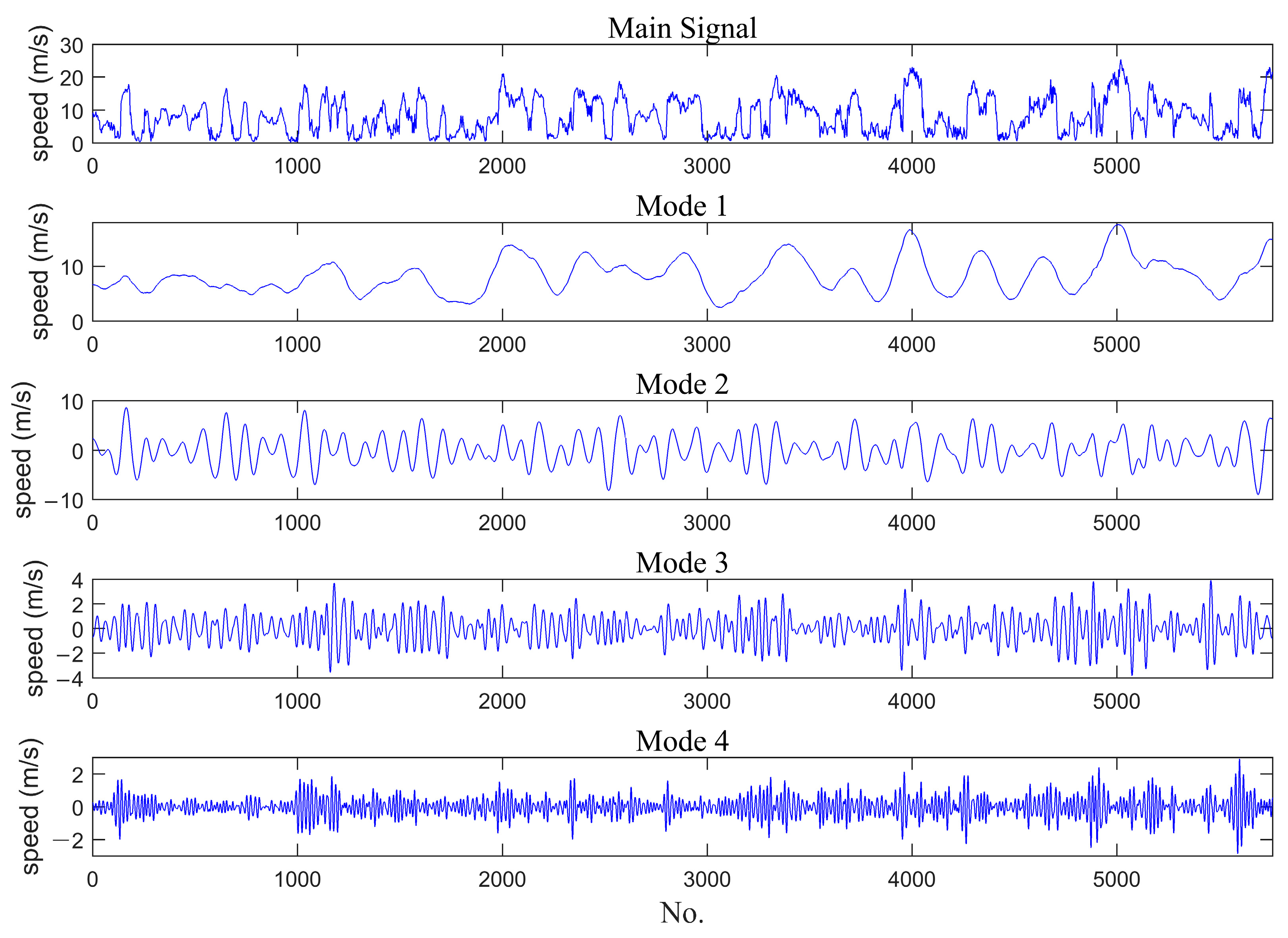
Wind speed time-series often contain different frequency components, including the trend term, cycle term and stochastic term, which hinders accurate modeling and forecasting. Through VMD, the historical speed wind data from a wind farm in Inner Mongolia, China together with four decomposed modes are shown in Figure 2. The original wind speed is extremely random and complex. Each decomposed mode is compacted around a center pulsation, and the higher order mode contains higher frequency components. The features of the trend components can be extracted from low frequency modes. The cycle term and stochastic term of wind speed can be predicted through modeling of the higher order modes.
3.2. Constitution of Input and Output Matrices
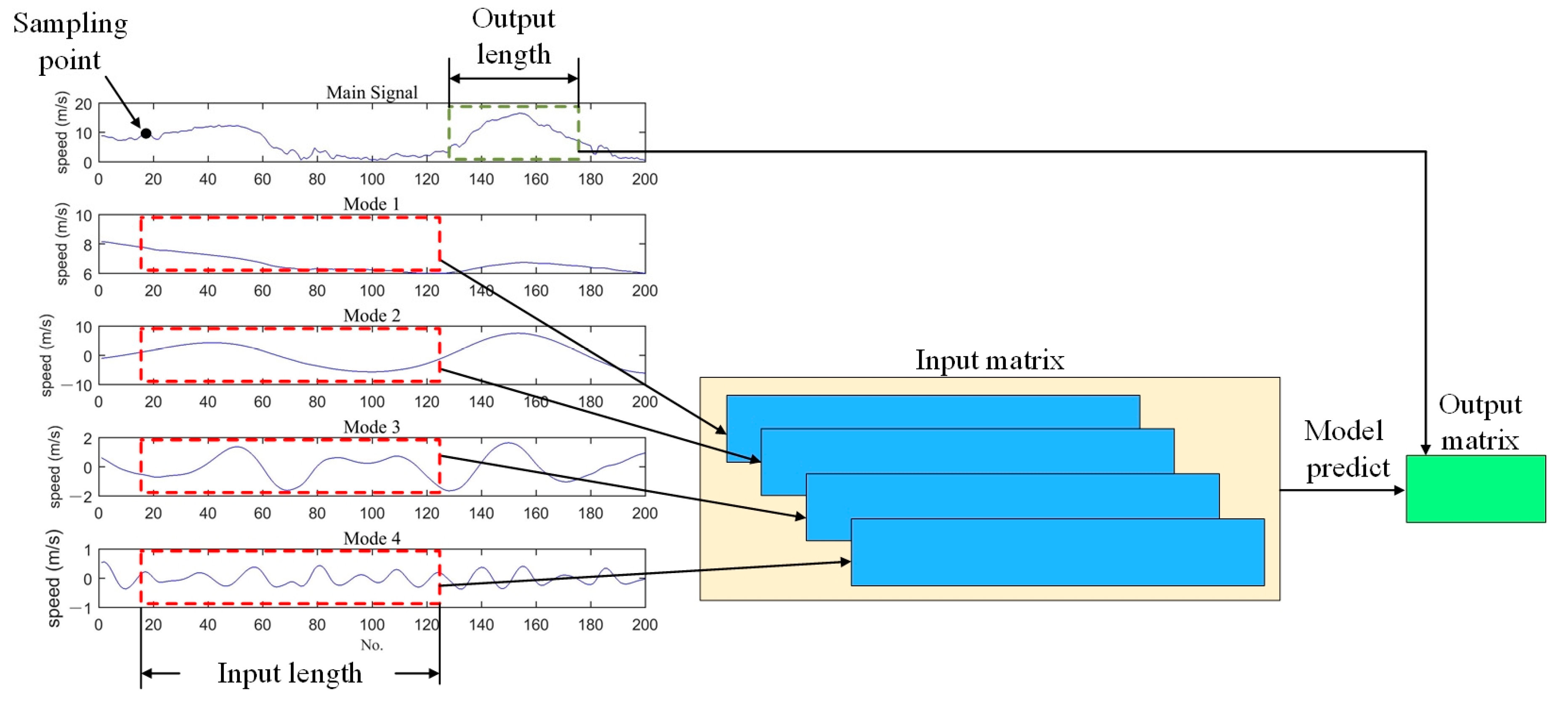
After decomposition of the wind speed data, modes in different frequency scales are obtained. As introduced in Section 2, the convolutional layers in CNN can be regarded as filters to extract local features from the input data. Therefore, the input and output matrices are constituted intuitively as illustrated in Figure 3. Let denote the k-th decomposed mode and denote the original wind speed signal, where L means the total number of observed points. Then, the input matrix Input and output matrix Output can be formulated as follows:
where and denote the input length and output length, respectively, i means the index of sampling point.
3.3. Forecasting Model Structure
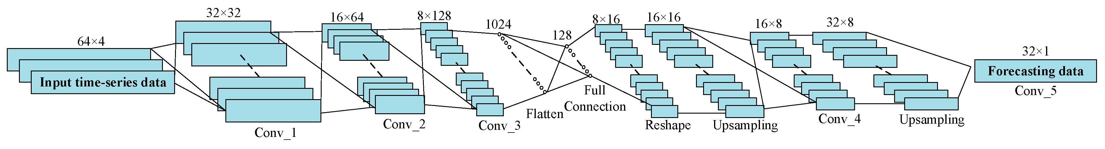
In this paper, 1-D CNN is adopted for wind speed forecasting. Common CNNs process images and accept input tensors in three dimensions, which are the width, height and number of color channels in images. Similarly, the 1-D CNN accepts time-series input in two dimensions: the time steps and number of channels. In fact, when the height of images is 1, the common CNN can be simplified to 1-D CNN. The CNN structure adopted in this paper is shown in Figure 4. The four channels in input data match the four decomposed modes from wind speed signal. Then, multiple filters extract features in different scale to capture the mapping relationship between input data and output data. The convolution of stride is employed instead of pooling (e.g., max pooling) because stride convolution is fully differentiable and allows the network to learn its own special down-sampling [17].
4. Applications to Wind Speed Forecasting
4.1. Data Description
In this paper, wind speed observation data gathered from a wind farm in Inner Mongolia, China were employed to demonstrate the efficiency of the proposed model. There was a total of 5760 points with a sampling interval of half an hour. We chose the first 4600 observations as the training set and the remaining points are used to test the model performance. The statistical information foreach data set is illustrated in Table 1. Before the training, the training set is normalized to enhance the CNN training performance. Besides, several classical statistical and their hybrid methods are constructed for comparison with our proposed model to evaluate the performance.
4.2. Model Establishment
There are two parameters that mainly influence the forecasting results of the proposed methods: the number of decomposed modes and the input length. The training data set was adopted to verify the structure of CNN. All the following experiments were run in Python 2.7 code. The Central Processing Unit (CPU) of the runtime environment was Intel Xeon E5-2650 v2 and the size of Random Access Memory (RAM) was 128 GB. The training data set was processed as described in Section 3. The parameters of each layer in the network were initialized through sampling from a random Gaussian distribution with zero mean and 0.1 standard deviation. In each experiment, the training iterations and output predicting length were kept the same, which were 100 epochs and 32, respectively. Considering the multi-step prediction output is a vector, the root mean squared error (RMSE) defined by the following is adopted to judge the predicting performance.
where M means the number of testing samples, and are the d-th predicting and true output of m-th sample, respectively.
4.2.1. Number of Decomposed Modes
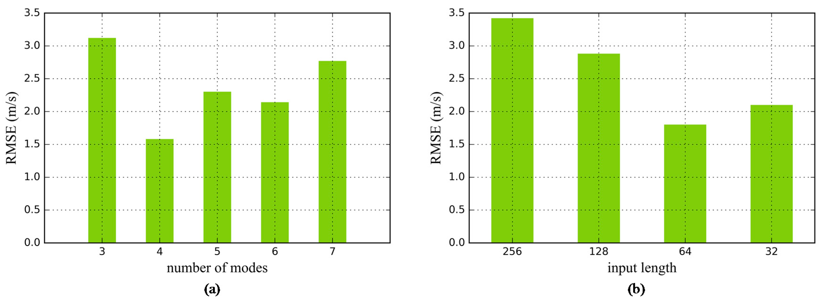
As mentioned above, mode mixing may appear and cause inaccurate prediction when the number of decomposed modes is too small. On the other side, too many modes will give rise to a complicated forecasting method and unnecessary computing overheads. To identify the channels of the input layer, the experiment was first conducted to observe the influence of number of decomposed modes. As illustrated in Figure 5a, the error comes to a minimum value when the number of decomposed modes is four. With the increase in number of modes, the predicting error increases from 1.59 to 2.78. When the wind speed signal is decomposed into 3 modes, the predicting error increases to 3.13. Therefore, the most suitable number of decomposed modes is chosen as 4 for the rest of the experiments.
4.2.2. Input Length
The determination of input length is another critical issue which not only decides the input layer of adopted forecasting structure but also influences the prediction results. As stride technology is employed in this model, the input length should be a power of 2 which is useful for construction. Hence, we choose 256, 128, 64 and 32 as the input length for comparison. In Figure 5b, the prediction error decreases from 3.43 to 1.81 when the input length ranges from 256 to 64. This phenomenon indicates that the long input tensors bring about extra noise for accurate forecasting. However, when the input length is the same as the output length, the prediction error increases to 2.11, which means that essential information about the relationship between the current data and historical data is lacking in this situation.
Therefore, the details of the adopted model are determined through the experiments described above. The number of decomposed modes is 4 and the input length is set as 64. The details of the forecasting model are shown in Table 2. As illustrated in Figure 5, although different parameters of VMD and input length influence the forecasting results, the CNN-based forecasting model generally achieved satisfactory results. Owing to the strong nonlinear learning and fitting ability, the proposed CNN is significantly better than some hybrid forecasting methods which are sensitive to the change in parameters.
4.3. Forecasting Results and Analysis
To verify the effectiveness of the proposed VMD-CNN method, the following experiments were conducted to compare it with some other existing methods that have been proved feasible for wind speed forecasting. The SVR is an efficient machine learning method for regression. The input matrices of SVRs were determined by partial autocorrelation function (PACF) values [13], and the parameters of SVRs were selected through grid search (GS). The ELM is a feed-forward network with a single hidden layer and is easy to train due to its fast convergence speed. In the case of ELM forecasting, the input matrices were the same as SVRs. GS was also used to optimize the number of hidden nodes, ranging from 20 to 1000. NN as a simplification of CNN, is also employed for comparison. Different from the case of SVR and ELM, the output of NN can be in multiple dimensions. The topology of NN was 64-100-100-32, and both hidden layers were activated by the ReLU activation function. The training epoch and optimization algorithm were the same as the proposed method. The CNN method without VMD had one channel instead of four and accepted the original data as input. The rest of the layers of CNN were the same as the proposed VMD-CNN model.
In the case of multi-step forecasting, we selected 16 h as the forecast horizon, which means all the methods were tested through generating 32 predictions from historical data. In order to obtain multiple step prediction results, iterative prediction was employed for the ELM and SVR methods, which means that one forecasting point was added into the input to constitute a new testing example until the length of the predicting output is the same as the proposed method. The output dimensions of NN were directly set as the output length while in the case of single-step forecasting, the output dimensions of NN was 1 and the outputs of CNN models were sent to a full connection layer with one-dimension. For each aforementioned forecasting approach, there was a VMD-based hybrid method for comparison and to exhibit the effectiveness of decomposition. For example, VMD-SVR means four SVR models were trained for four decomposed modes and the prediction results were obtained by aggregating each prediction value.
Three common evaluating indicators were adopted to estimate the performance of the forecasting models. The RMSE is defined as Equation (10), while the mean absolute error (MAE) and mean absolute percentage error (MAPE) are formulated as follows:
In addition, the improved percentage of RMSE, MAE, MAPE are exploited to intuitively describe the degree of enhancement from model 1 to model 2. The definitions are as the follows:
where , , , , and are the errors of model 1 and model 2, respectively.
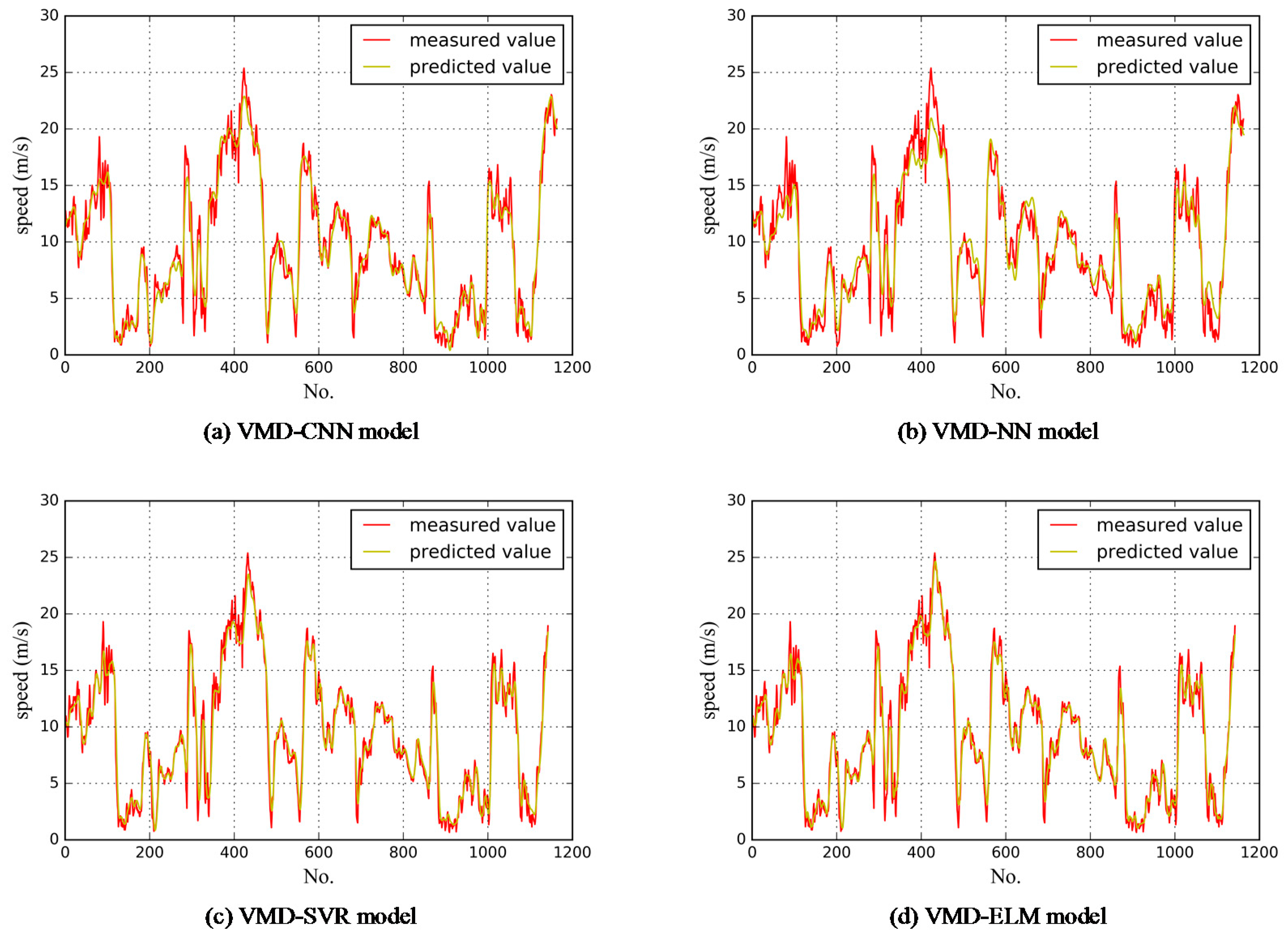
The final results are shown in Table 3 and illustrated in Figure 6. In the single-step forecasting experiment, all the VMD-based hybrid methods had a better performance compared with their statistical method. The RMSE decreases 0.61, 0.75, 0.35 and 0.18 for SVR, ELM, NN, CNN and their hybrid method, respectively. This phenomenon proves that the decomposition of signal is helpful for single-step forecasting because the simpler vibration mode of decomposed modes is easier to predict. It can be seen that the VMD-SVR hybrid method performs the best in RMSE, MAE and MAPE. Although the errors of other methods are greater, the maximum RMSE, MAE and MAPE values among them are also satisfactory, which are 1.64, 1.36 and 22.88 respectively. The forecasting results of all the hybrid methods are presented in Figure 7. All of them can approximately fit the test data with very little error. Therefore, multi-step forecasting is more worthy of research and development for short-term wind speed forecasting.
In the multi-step forecasting experiment, the SVR and ELM, which are the single-step predicting methods, underperformed significantly. The applied iterative predicting approach accumulates a little error in each step, and finally leads to a significant error. The NN and CNN can directly output predictions in multiple dimensions owing to their architecture. Thus, in the case of multi-step forecasting, the NN and CNN based methods performed much better than SVR and ELM. As illustrated in Figure 6 and Table 3, the proposed VMD-CNN method achieved the best result among all the methods. The RMSE, MAE and MAPE of VMD-CNN are 1.3, 1.04 and 20.31, respectively which are roughly the same as the single-step experiment. By contrast, the RMSE, MAE and MAPE of VMD-SVR increase to 6.36, 5.04 and 89.22, respectively.
In addition, the improved percentages between the proposed VMD-CNN method and the other methods are shown in Table 4. It is clearly shown that the proposed method performs 72.22%, 79.33%, 40.91% and 70.18% better for RMSE than SVR, ELM, VMD-NN and CNN, respectively. A great improvement also exits for MAE and MAPE indexes. This result verifies the significant superiority of the proposed method in multi-step wind speed forecasting. It is worth noting that the SVR and ELM perform better than their hybrid VMD-based methods, which means their multi-step forecasting performance on decomposed modes are also not good enough. By contrast, the hybrid VMD-based NN and CNN methods can enhance RMSE by 52.99% and 72.18%compared to NN and CNN methods, respectively.
Finally, some random test examples were chosen and their multi-step prediction results for SVR, ELM, VMD-NN and the proposed VMD-CNN methods are shown in Figure 8. In Figure 8, the cumulative processes of errors of SVR and ELM are clearly exhibited. At the beginning of the iterations, the SVR and ELM methods can accurately predict the future value. With the increases in iteration, the prediction results of SVR and ELM methods are uncontrollable and far from the true value. The VMD-NN and VMD-CNN methods can basically forecast the change of wind speed and VMD-CNN performs better in the majority of examples. In fact, the proposed VMD-CNN method can accurately predict the variation trends in wind speed ignoring the slight randomness. Therefore, these multi-step forecasting results strongly suggest the significance of the proposed method for multi-step wind speed forecasting.
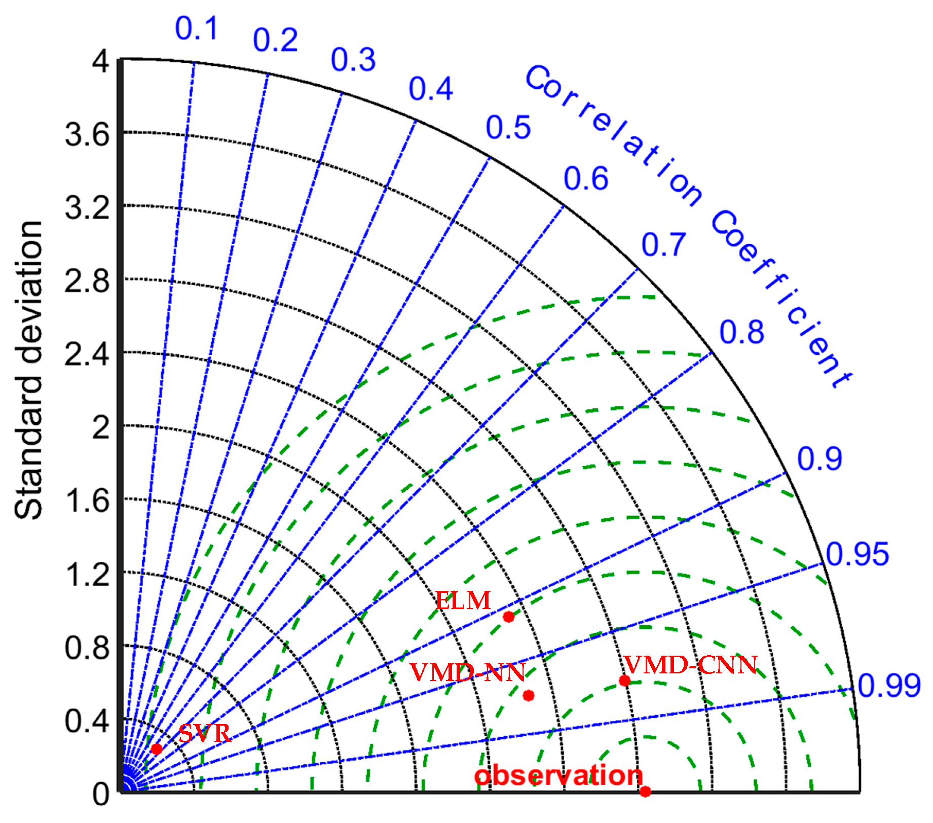
In order to specifically describe the prediction results of different models, a Taylor diagram is employed as illustrated in Figure 9. The standard deviations, centered root-mean-square and pattern correlations with observation of each prediction in testing example 1 are clearly exhibited. In Figure 9, it can be seen that the VMD-NN and VMD-CNN model have roughly the same correlation coefficient as the observation. However, the VMD-CNN model has the smallest RMSE and the same standard deviation as the observation, whereas the VMD-NN model has little spatial variability, considering its smaller standard deviations. Of the poorer performing models, the ELM model is most correlative with observation, while the standard deviation of the SVR model is close to zero, which means the prediction of the SVR model stays the same without variation. In general, our proposed VMD-CNN model outperforms the compared models on all of the statistical characteristics.
4.4. Additional Forecasting Case
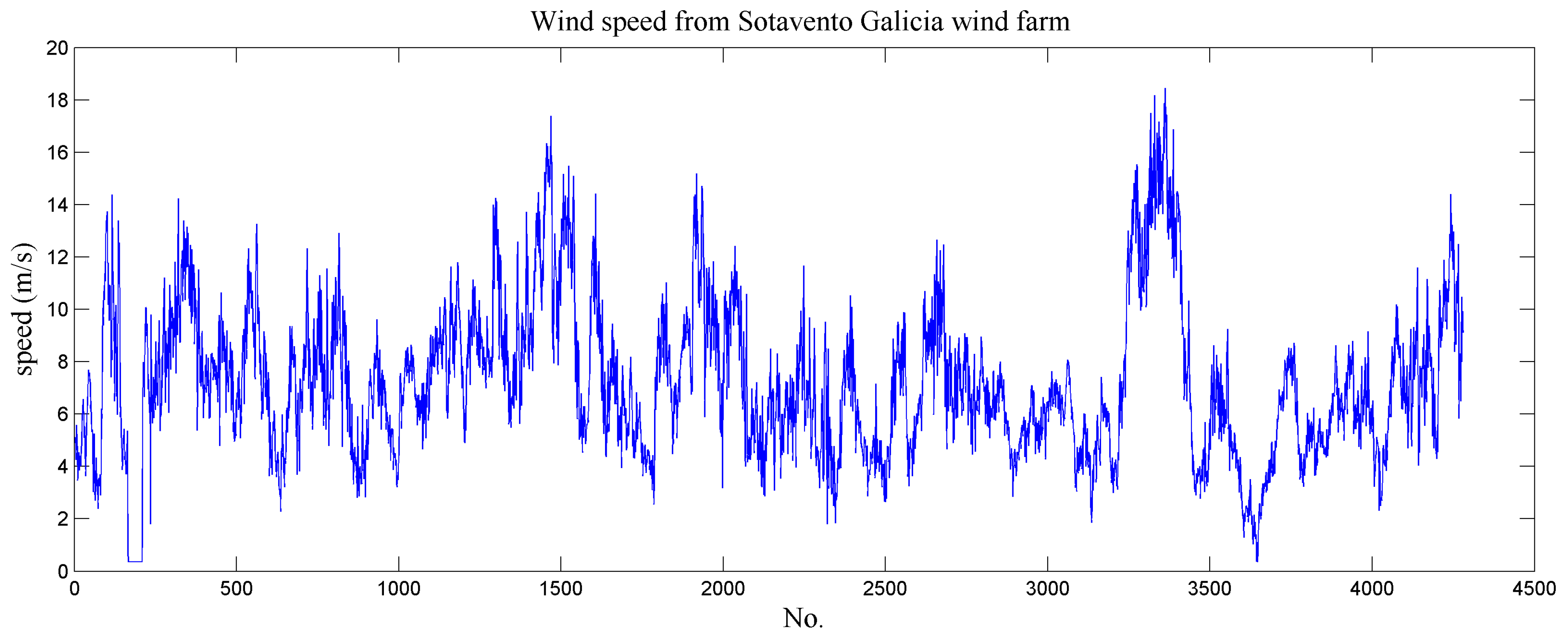
In order to further verify the efficiency of the proposed method, the 10-min wind speed data of the widely-studied wind farm in Sotavento Galicia, Spain [31] collected from 1 March 2018 to 31 March 2018 were used as an additional multi-step forecasting case. The number of observations for wind speed included in this study amounts to 4280. The first 3200 points were chosen for training and the remaining data are used to verify the performance of the models. The original observations are shown in Figure 10 and the statistical information is listed in Table 5. We chose SVR and ELM models for comparison in this study because their performances are better than their hybrid model in the multi-step forecasting experiment. Like the experiment for wind speed data in Inner Mongolia, China, the output length of all models was 32, which meant the forecast horizon was 5.3 h. The RMSE, MAE and MAPE of the different methods are listed in Table 6. As illustrated in Table 6, the rankings of the forecasting results are similar to the one in Section 4.3. The proposed method still has the best performance among all of the tested models. These results have demonstrated that the proposed method has immense potential for multi-step wind speed forecasting.
5. Conclusions
This paper proposes a hybrid method for multi-step wind speed forecasting. The proposed VMD-CNN method employs VMD to decompose the wind speed signal into different modes under different center pulsation. By taking advantage of the structure of CNN, each mode is regarded as one channel to constitute the input. Then, the filters in each layer of CNN are trained to extract the local features and relationships between modes. Finally, the output layer of CNN is set in multiple dimensions to directly forecast the future wind speed. Several experiments were conducted to prove the effectiveness of the proposed method. By comparing the statistical approaches and their hybrid VMD-based methods, it has been proved that the decomposed modes are helpful for accurate predicting. Although the ELM and SVR methods performed better in single-step forecasting, the proposed method also exactly predicted the next wind speed value. In the case of multi-step forecasting, the proposed method achieved significant results while the SVR-based and ELM-based methods performed poorly. The VMD-CNN method predicted the variation trend of wind speed in general. For every evaluating indicator, our proposed VMD-CNN achieved the lowest value. However, the number and size of the filters of the proposed method should be optimized to adapt to more complicated wind speed. The influence of other signal process approaches should be discussed specifically in the future. For further studies, the impact of other climate parameters, such as wind direction could also be considered as an input or output to enhance the forecasting performance.
Author Contributions
J.Z. and H.L. designed and performed the forecasting model; Y.X. and W.J. analyzed the data; H.L. and W.J. wrote the paper.
Funding
This research was funded by the National Key R&D Program of China (Nos. 2016YFC0402205, 2016YFC0401910), the National Natural Science Foundation of China (Nos. 51579107, 51079057) and the Natural Science Foundation of Huazhong University of Science and Technology (No. 2017KFYXJJ209).
Acknowledgments
This work was supported by the National Key R&D Program of China (Nos. 2016YFC0402205, 2016YFC0401910), the National Natural Science Foundation of China (NSFC) (Nos. 51579107, 51079057) and the Natural Science Foundation of Huazhong University of Science and Technology (No. 2017KFYXJJ209).
Conflicts of Interest
The authors declare no conflict of interest.
Nomenclature
| the corresponding activation output of convolutional layer | |
| the original signal | |
| Input | the input matrix of the proposed model |
| K | the number of decomposed modes |
| L | the total number of observed points |
| the length of input data in our proposed model | |
| the length of forecasting data in our proposed model | |
| M | the number of testing samples |
| MAE | the mean absolute error |
| MAPE | the mean absolute percentage error |
| Output | the output matrix of the proposed model |
| the improved percentage of RMSE | |
| the improved percentage of MAE | |
| the improved percentage of MAPE | |
| RMSE | the root mean squared error |
| the d-th predicting value of m-th sample | |
| the k-th decomposed modes | |
| the parameters of i-th filter kernel in l-th layer | |
| the input of a layer in network | |
| the input in local region j of layer l | |
| the output of a layer in network | |
| the d-th true value of m-th sample | |
| the corresponding output of local region j of layer l through convolutional layer | |
| the balancing parameter | |
| the Dirac distribution | |
| center pulsation of | |
| the noise-tolerance | |
| the tolerance of convergence criterion | |
| * | convolution operation |
| Euclidean distance |
References
- Ponta, L.; Raberto, M.; Teglio, A.; Cincotti, S. An Agent-based Stock-flow Consistent Model of the Sustainable Transition in the Energy Sector. Mpra Paper 2016, 145, 274–300. [Google Scholar] [CrossRef]
- Soman, S.S.; Zareipour, H.; Malik, O.; Mandal, P. A review of wind power and wind speed forecasting methods with different time horizons. In Proceedings of the North American Power Symposium, Arlington, TX, USA, 26–28 September 2010; pp. 1–8. [Google Scholar]
- Landberg, L. Short-term prediction of the power production from wind farms. J. Wind Eng. Aerodyn. 1999, 80, 207–220. [Google Scholar] [CrossRef]
- Lazić, L.; Pejanović, G.; Živković, M. Wind forecasts for wind power generation using the Eta model. Renew. Energy 2010, 35, 1236–1243. [Google Scholar] [CrossRef]
- Potter, C.W.; Negnevitsky, M. Very short-term wind forecasting for Tasmanian power generation. IEEE Trans. Power Syst. 2006, 21, 965–972. [Google Scholar] [CrossRef]
- Torres, J.L.; García, A.; Blas, M.D.; Francisco, A.D. Forecast of hourly average wind speed with ARMA models in Navarre (Spain). Sol. Energy 2005, 79, 65–77. [Google Scholar] [CrossRef]
- Cadenas, E.; Rivera, W. Wind speed forecasting in the South Coast of Oaxaca, México. Renew. Energy 2007, 32, 2116–2128. [Google Scholar] [CrossRef]
- Weron, R. Electricity price forecasting: A review of the state-of-the-art with a look into the future. Int. J. Forecast. 2014, 30, 1030–1081. [Google Scholar] [CrossRef]
- Hinton, G.E.; Salakhutdinov, R.R. Reducing the Dimensionality of Data with Neural Networks. Science 2006, 313, 504–507. [Google Scholar] [CrossRef] [PubMed]
- Barbounis, T.G.; Theocharis, J.B.; Alexiadis, M.C.; Dokopoulos, P.S. Long-term wind speed and power forecasting using local recurrent neural network models. IEEE Trans. Energy Convers. 2006, 21, 273–284. [Google Scholar] [CrossRef]
- Mikolov, T.; Karafiát, M.; Burget, L.; Černocký, J.; Khudanpur, S. Recurrent Neural Network Based Language Model. In Proceedings of the INTERSPEECH 2010 11th Annual Conference of the International Speech Communication Association, Makuhari, Japan, 26–30 September 2010; pp. 1045–1048. [Google Scholar]
- López, E.; Valle, C.; Allende, H.; Gil, E.; Madsen, H. Wind Power Forecasting Based on Echo State Networks and Long Short-Term Memory. Energies 2018, 11, 526. [Google Scholar] [CrossRef]
- Zhang, C.; Zhou, J.; Li, C.; Fu, W.; Peng, T. A compound structure of ELM based on feature selection and parameter optimization using hybrid backtracking search algorithm for wind speed forecasting. Energy Convers. Manag. 2017, 143, 360–376. [Google Scholar] [CrossRef]
- Huang, G.B.; Zhu, Q.Y.; Siew, C.K. Extreme learning machine: Theory and applications. Neurocomputing 2006, 70, 489–501. [Google Scholar] [CrossRef] [Green Version]
- Cincotti, S.; Gallo, G.; Ponta, L.; Raberto, M. Modeling and forecasting of electricity spot-prices: Computational intelligence vs. classical econometrics. Ai Commun. 2014, 27, 301–314. [Google Scholar]
- Fu, W.; Zhou, J.; Zhang, Y.; Zhu, W.; Xue, X.; Xu, Y. A state tendency measurement for a hydro-turbine generating unit based on aggregated EEMD and SVR. Meas. Sci. Technol. 2015, 26, 125008. [Google Scholar] [CrossRef]
- Wang, J.; Wang, Y.; Li, Y. A Novel Hybrid Strategy Using Three-Phase Feature Extraction and a Weighted Regularized Extreme Learning Machine for Multi-Step Ahead Wind Speed Prediction. Energies 2018, 11, 321. [Google Scholar] [CrossRef]
- Liu, H.; Mi, X.; Li, Y. An experimental investigation of three new hybrid wind speed forecasting models using multi-decomposing strategy and ELM algorithm. Renew. Energy 2018, 123, 694–705. [Google Scholar] [CrossRef]
- Senjyu, T.; Yona, A.; Urasaki, N.; Funabashi, T. Application of Recurrent Neural Network to Long-Term-Ahead Generating Power Forecasting for Wind Power Generator. In Proceedings of the IEEE Power Systems Conference and Exposition, Atlanta, GA, USA, 29 October–1 November 2006; pp. 1260–1265. [Google Scholar]
- Abdoos, A.A. A new intelligent method based on combination of VMD and ELM for short term wind power forecasting. Neurocomputing 2016, 203, 111–120. [Google Scholar] [CrossRef]
- Naik, J.; Bisoi, R.; Dash, P.K. Prediction interval forecasting of wind speed and wind power using modes decomposition based low rank multi-kernel ridge regression. Renew. Energy 2018, 129, 357–383. [Google Scholar] [CrossRef]
- Radford, A.; Metz, L.; Chintala, S. Unsupervised Representation Learning with Deep Convolutional Generative Adversarial Networks. In Proceedings of the International Conference on Learning Representations, San Juan, Puerto Rico, 2–4 May 2016. [Google Scholar]
- Krizhevsky, A.; Sutskever, I.; Hinton, G.E. ImageNet classification with deep convolutional neural networks. In Proceedings of the International Conference on Neural Information Processing Systems, Stateline, NV, USA, 3–8 December 2012; pp. 1097–1105. [Google Scholar]
- Zhang, W.; Li, C.; Peng, G.; Chen, Y.; Zhang, Z. A deep convolutional neural network with new training methods for bearing fault diagnosis under noisy environment and different working load. Mech. Syst. Signal Process. 2018, 100, 439–453. [Google Scholar] [CrossRef]
- Kalchbrenner, N.; Grefenstette, E.; Blunsom, P. A Convolutional Neural Network for Modelling Sentences. In Proceedings of the Association for Computational Linguistics, Baltimore, MD, USA, 22–27 June 2014. [Google Scholar]
- Dragomiretskiy, K.; Zosso, D. Variational Mode Decomposition. IEEE Trans. Signal Process. 2014, 62, 531–544. [Google Scholar] [CrossRef]
- Zhang, Y.; Liu, K.; Qin, L.; An, X. Deterministic and probabilistic interval prediction for short-term wind power generation based on variational mode decomposition and machine learning methods. Energy Convers. Manag. 2016, 112, 208–219. [Google Scholar] [CrossRef]
- Lahmiri, S. Comparing Variational and Empirical Mode Decomposition in Forecasting Day-Ahead Energy Prices. IEEE Syst. J. 2017, 11, 1907–1910. [Google Scholar] [CrossRef]
- Zhang, X.; Miao, Q.; Zhang, H.; Wang, L. A parameter-adaptive VMD method based on grasshopper optimization algorithm to analyze vibration signals from rotating machinery. Mech. Syst. Signal Process. 2018, 108, 58–72. [Google Scholar] [CrossRef]
- Kingma, D.; Ba, J. Adam: A Method for Stochastic Optimization. In Proceedings of the 3rd International Conference for Learning Representations, San Diego, CA, USA, 7–9 May 2015. [Google Scholar]
- Lydia, M.; Suresh Kumar, S.; Immanuel Selvakumar, A.; Edwin Prem Kumar, G. Linear and non-linear autoregressive models for short-term wind speed forecasting. Energy Convers. Manag. 2016, 112, 115–124. [Google Scholar] [CrossRef]
Figure 1.
The architecture of the proposed variational mode decomposition (VMD)-convolutional neural network (CNN) hybrid data-driven forecasting model.
Figure 1.
The architecture of the proposed variational mode decomposition (VMD)-convolutional neural network (CNN) hybrid data-driven forecasting model.
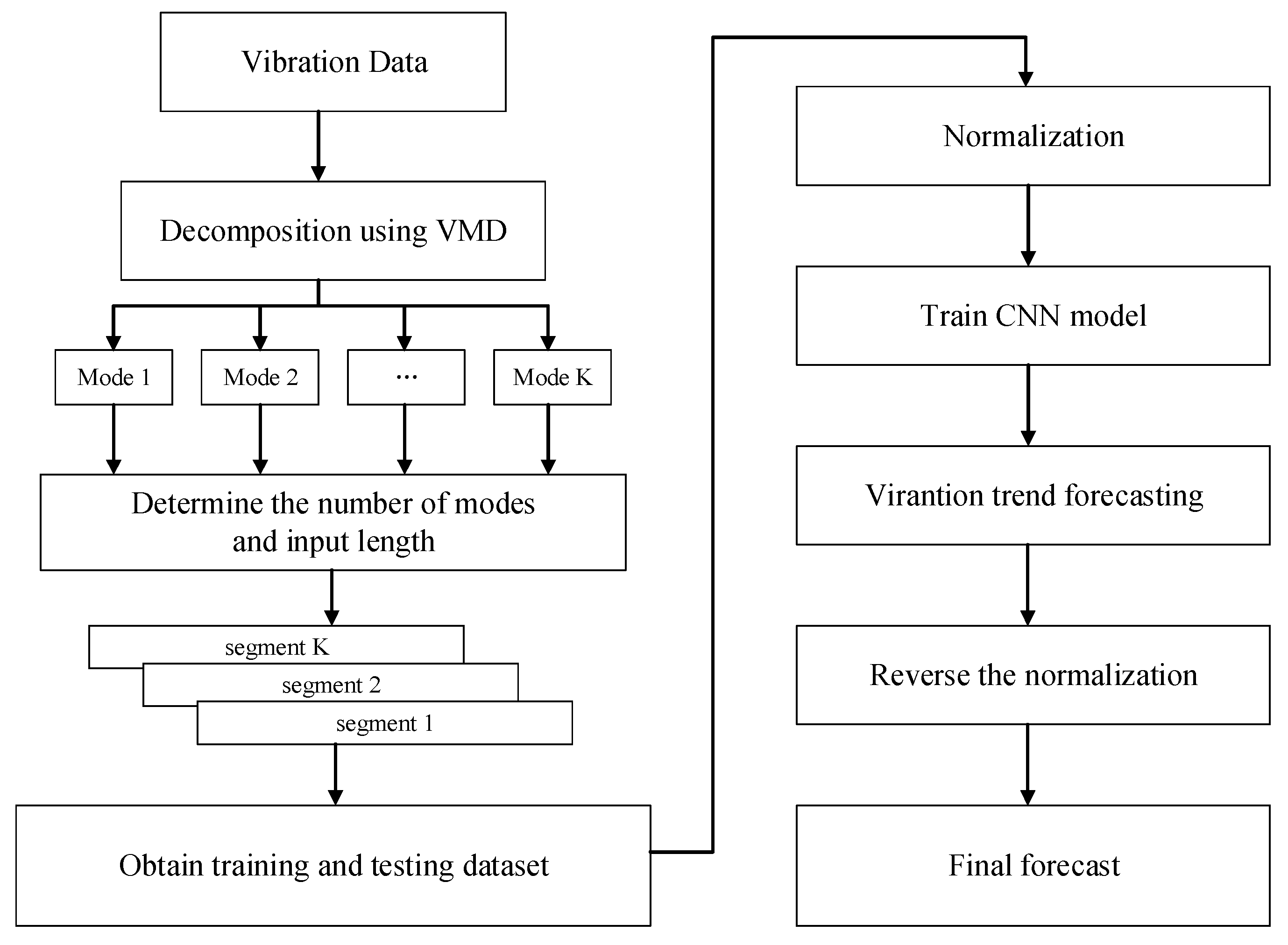
Figure 2.
Wind speed signal and the decomposed modes.

Figure 3.
Constitution of input and output matrices.

Figure 4.
Structure of the CNN model adopted for forecasting.

Figure 5.
Comparison of different model parameters: (a) number of modes, (b) input length.

Figure 6.
Evaluating indicators of forecasting models: (a) multi-step forecasting, (b) single-step forecasting. RMSE: root mean squared error; MAE: mean absolute error; MAPE: mean absolute percentage error.
Figure 6.
Evaluating indicators of forecasting models: (a) multi-step forecasting, (b) single-step forecasting. RMSE: root mean squared error; MAE: mean absolute error; MAPE: mean absolute percentage error.
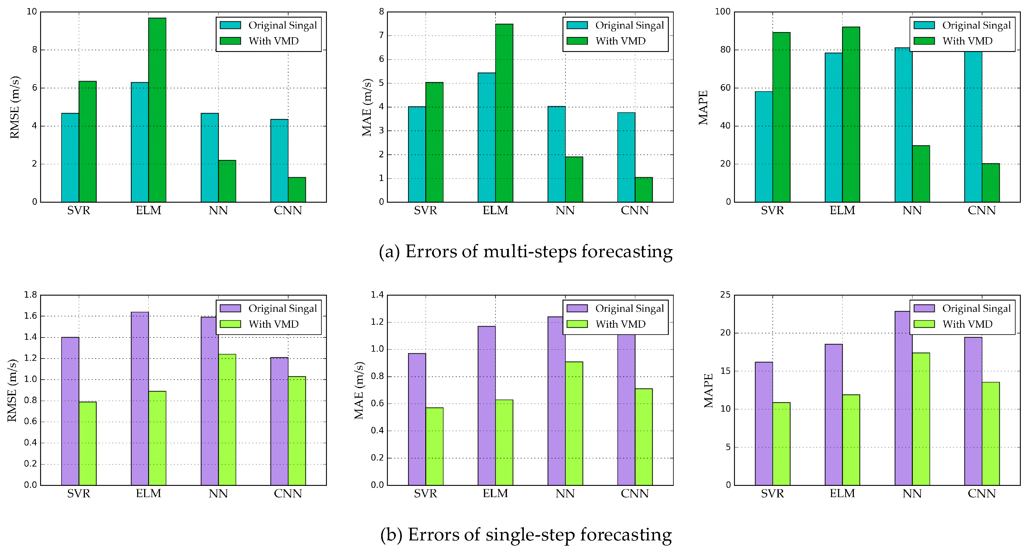
Figure 7.
The single-step forecasting results of hybrid methods: (a) VMD-CNN model, (b) VMD-NN model, (c) VMD-SVR model, (d) VMD-ELM model NN: neural networks; SVR: support vector regression; ELM: extreme learning machine.
Figure 7.
The single-step forecasting results of hybrid methods: (a) VMD-CNN model, (b) VMD-NN model, (c) VMD-SVR model, (d) VMD-ELM model NN: neural networks; SVR: support vector regression; ELM: extreme learning machine.

Figure 8.
The multi-step forecasting results of the methods.
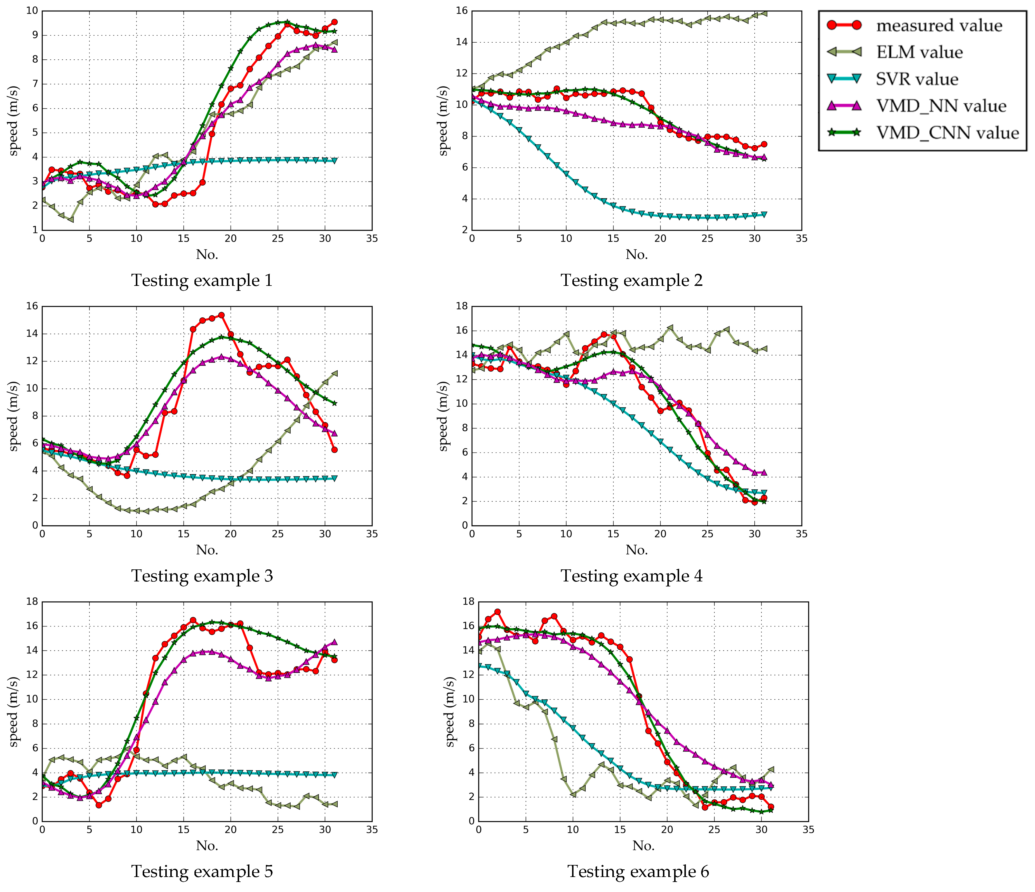
Figure 9.
Taylor diagram of testing example 1.

Figure 10.
Wind speed time-series of Sotavento Galicia wind farm.

Table 1.
Statistical information for each data set.
| Statistical Indicator | Entire Data Set | Training Data Set | Testing Data Set |
|---|---|---|---|
| Maximum (m/s) | 25.39 | 23.10 | 25.39 |
| Minimum (m/s) | 0.3 | 0.3 | 0.66 |
| Median (m/s) | 7.81 | 7.45 | 9.02 |
| Mean (m/s) | 8.28 | 7.916 | 9.732 |
| Standard deviation (m/s) | 5.262 | 5.074 | 5.726 |
| Coefficient of variation (%) | 63.55 | 64.10 | 58.84 |
| Autocorrelation function value at lag 1 | 0.9886 | 0.9892 | 0.986 |
Table 2.
Forecasting model details.
| No. | Layer Type | Output Dimensions | Kernel Size | Kernel Number | Stride | Activation Function |
|---|---|---|---|---|---|---|
| 1 | Input layer | 64 × 4 | / | / | / | / |
| 2 | Convolutional layer 1 | 32 × 32 | 20 | 32 | 2 | ReLU |
| 3 | Convolutional layer 2 | 16 × 64 | 10 | 64 | 2 | ReLU |
| 4 | Convolutional layer 3 | 8 × 128 | 5 | 128 | 2 | ReLU |
| 5 | Flatten | 1024 | / | / | / | / |
| 6 | Full Connection | 128 | / | / | / | ReLU |
| 7 | Reshape | 8 × 16 | / | / | / | / |
| 8 | UpSampling | 16 × 16 | / | / | / | / |
| 9 | Convolutional layer 4 | 16 × 8 | 5 | 8 | 1 | ReLU |
| 10 | UpSampling | 32 × 8 | / | / | / | / |
| 11 | Convolutional layer 5 | 32 × 1 | 10 | 1 | 1 | linear |
Adam’s [30] optimization algorithm is adopted to update the parameters in each layers. ReLU: rectified linear unit.
Table 3.
Multi-step and single-step forecasting results of different methods.
| Method | Multi-Step Forecasting | Single-Step Forecasting | ||||
|---|---|---|---|---|---|---|
| RMSE (m/s) | MAE (m/s) | MAPE (%) | RMSE (m/s) | MAE (m/s) | MAPE (%) | |
| SVR | 4.68 | 4.02 | 58.18 | 1.40 | 0.97 | 16.19 |
| VMD-SVR | 6.36 | 5.04 | 89.22 | 0.79 | 0.57 | 10.88 |
| ELM | 6.29 | 5.44 | 78.43 | 1.64 | 1.17 | 18.55 |
| VMD-ELM | 9.68 | 7.49 | 92.16 | 0.89 | 0.63 | 11.91 |
| NN | 4.68 | 4.03 | 81.22 | 1.59 | 1.24 | 22.88 |
| VMD-NN | 2.20 | 1.91 | 29.80 | 1.24 | 0.91 | 17.38 |
| CNN | 4.36 | 3.77 | 88.04 | 1.21 | 1.36 | 19.46 |
| VMD-CNN | 1.30 | 1.04 | 20.31 | 1.03 | 0.71 | 13.55 |
RMSE: root mean squared error; MAE: mean absolute error; MAPE: mean absolute percentage error.
Table 4.
Improved percentages of different methods in multi-step forecasting.
| Compared Methods | PRMSE | PMAE | PMAPE |
|---|---|---|---|
| VMD-CNN vs. SVR | 72.22 | 74.12 | 65.09 |
| VMD-CNN vs. ELM | 79.33 | 80.88 | 74.10 |
| VMD-CNN vs. VMD-NN | 40.91 | 45.54 | 31.85 |
| VMD-CNN vs. CNN | 70.18 | 72.41 | 76.93 |
| SVR vs. VMD-SVR | 26.41 | 20.23 | 34.79 |
| ELM vs. VMD-ELM | 35.02 | 27.36 | 14.89 |
| VMD-NN vs. NN | 52.99 | 52.60 | 66.59 |
NN: neural networks; SVR: support vector regression; ELM: extreme learning machine.
Table 5.
Statistical information of wind speed from Sotavento Galicia wind farm.
| Statistical Indicator | Entire Data Set | Training Data Set | Testing Data Set |
|---|---|---|---|
| Maximum (m/s) | 18.46 | 18.46 | 14.40 |
| Minimum (m/s) | 0.35 | 0.35 | 0.35 |
| Median (m/s) | 6.75 | 7.01 | 5.9 |
| Mean (m/s) | 7.16 | 7.42 | 6.06 |
| Standard deviation (m/s) | 2.913 | 2.637 | 3.610 |
| Coefficient of variation (%) | 40.70 | 35.54 | 59.57 |
| Autocorrelation function value at lag 1 | 0.9397 | 0.9354 | 0.9372 |
Table 6.
Multi-step forecasting results of models in Sotavento Galicia wind farm.
| Method | Multi-Step Forecasting | ||
|---|---|---|---|
| RMSE (m/s) | MAE (m/s) | MAPE (%) | |
| SVR | 3.57 | 3.35 | 50.56 |
| ELM | 4.55 | 4.21 | 65.93 |
| VMD-NN | 1.77 | 1.41 | 45.31 |
| VMD-CNN | 1.21 | 0.95 | 23.14 |
© 2018 by the authors. Licensee MDPI, Basel, Switzerland. This article is an open access article distributed under the terms and conditions of the Creative Commons Attribution (CC BY) license (http://creativecommons.org/licenses/by/4.0/).
Share and Cite
MDPI and ACS Style
Zhou, J.; Liu, H.; Xu, Y.; Jiang, W. A Hybrid Framework for Short Term Multi-Step Wind Speed Forecasting Based on Variational Model Decomposition and Convolutional Neural Network. Energies 2018, 11, 2292. https://doi.org/10.3390/en11092292
AMA Style
Zhou J, Liu H, Xu Y, Jiang W. A Hybrid Framework for Short Term Multi-Step Wind Speed Forecasting Based on Variational Model Decomposition and Convolutional Neural Network. Energies. 2018; 11(9):2292. https://doi.org/10.3390/en11092292
Chicago/Turabian StyleZhou, Jianzhong, Han Liu, Yanhe Xu, and Wei Jiang. 2018. "A Hybrid Framework for Short Term Multi-Step Wind Speed Forecasting Based on Variational Model Decomposition and Convolutional Neural Network" Energies 11, no. 9: 2292. https://doi.org/10.3390/en11092292
Note that from the first issue of 2016, this journal uses article numbers instead of page numbers. See further details here.