A Modified Firefly Algorithm with Rapid Response Maximum Power Point Tracking for Photovoltaic Systems under Partial Shading Conditions

Abstract

A rapid response optimization technique for photovoltaic maximum power point tracking (MPPT) under partial shading conditions (PSCs) is proposed in this study. To improve the solar MPPT tracking speed for rapidly-changing environmental conditions and to prevent the conventional firefly algorithm (FA) from becoming trapped at the local peaks and oscillations during the search process, a novel fusion algorithm, named the modified firefly algorithm (MFA), is proposed. The MFA integrates and modifies the processes of two algorithms, namely the firefly algorithm with neighborhood attraction (NaFA) and simplified firefly algorithm (SFA). A modified attraction process for the NaFA is used in the first iteration to avoid trapping at local maximum power points (LMPPs). In addition, in order to improve the convergence speed, the attractiveness factor of the attraction process is designed to be related to the power and position difference of the fireflies. Furthermore, the number of fireflies is designed to decrease in proportion with the iterations in the modified SFA process. Results from both the simulations and evaluations verify that the proposed algorithm offers rapid response with high accuracy and efficiency when encountering PSCs. In addition, the MFA can avoid becoming trapped at LMPPs and ease the oscillations during the search process. Consequently, the proposed method could be considered to be one of the most promising substitutes for existing approaches. In addition, the proposed method is adaptable to different types of solar panels and different system formats with specifically designed parameters.

1. Introduction

The power-voltage characteristics (P-V curve) of a photovoltaic (PV) system are nonlinear and influenced by both the solar irradiance and ambient temperature, which exhibit different maximum power points (MPPs). In order to optimize the utilization of PV systems, conventional maximum power-point tracking (MPPT) algorithms, such as perturb and observe (P&O), Incremental Conductance (IC), and Hill Climbing (HC), are frequently utilized [1,2,3]. However, when PV modules become fractionally shaded and receive varying amounts of solar irradiance due to clouds, trees, tall buildings, and/or other neighboring objects, partial shading conditions (PSCs) occur and cause the P-V curves of the PV modules to exhibit multiple local maximum power points (LMPPs) [4,5]. Another cause of PSCs is randomness in the PV modules themselves, such as the occurrence of cracks in the PV panels [6]. Under PSCs, conventional MPPT methods can easily fail to identify the global maximum power point (GMPP) among the numerous LMPPs and then become trapped at a local peak, which might significantly reduce the output power of the PV modules. Moreover, environmental conditions often change rapidly; therefore, improving the tracking speed of MPPT algorithms under PSCs has received much attention in recent years [7].

Nature-inspired algorithms have drawn increasing attention from researchers for MPPT application under PSCs, as they properly deal with non-linear and stochastic optimization problems and offer excellent performance without involving complex mathematical calculations, resulting in computational simplicity and quick response [6,8]. Various nature-inspired algorithms, such as the particle swarm optimization (PSO) [9], the flower pollination algorithm (FPA) [10,11], and the firefly algorithm (FA) [12,13] have been verified to handle the MPPT optimization problem well under PSCs. Among those techniques, PSO has the advantages of simple structure, straightforward experimental implementation, and high accuracy. However, the convergence speed of this method is slow due to the complex computation processes [10,13,14]. Although the tracking accuracy of the FPA is high, the stability of its convergence speed is low due to the Levy distribution of the cross-pollination process.

The FA is an effective optimization technique based on the light-intensity behavior of fireflies, and it has been confirmed to accurately track the GMPP under PSCs. The major advantages of adopting the FA for solar MPPT are its high accuracy, simple computational processes, fast convergence and lower PV-power turbulence [6,13]. Nevertheless, too many attractions during the conventional FA search process may cause the fireflies to become trapped in the LMPPs or result in oscillations [15]. In addition, the tracking speed of the FA could be further improved for solar MPPT applications, especially under rapidly-changing environmental conditions. The simplified firefly algorithm (SFA), which is a modification of the FA, has been proposed in order to improve the tracking speed by simplifying the convergence process [16]; nevertheless, this comes at the cost of decreased tracking accuracy and even more frequent trapping at LMPPs [6]. In response, the firefly algorithm with the neighborhood attraction (NaFA) algorithm was proposed to mitigate the over-attraction problem of the FA [15]. When compared with the SFA, the NaFA can efficiently improve the tracking accuracy, but it has slower convergence speed.

In order to improve both the tracking speed and accuracy of the FA, a modified firefly algorithm (MFA) that integrates the processes of the NaFA and SFA is proposed in this study. A modified attraction process for the NaFA is used in the first iteration to avoid trapping at LMPPs. In this study, the attractiveness factor of the attraction process is specifically designed to be related to the power and location difference of the fireflies, which can improve its processing speed. For the second and following iterations, a modified SFA with convergence-speed-improved processes is implemented. The number of fireflies is designed to decrease in proportion with the iterations, which improves the convergence speed. To our knowledge, this is the first study that evaluates the fusion of the NaFA and SFA for photovoltaic MPPT [6,17]. The advantages of the proposed algorithm are rapid response time with high accuracy and efficiency for PV systems under PSCs.

2. Methodology

2.1. Solar Cell Circuit Model

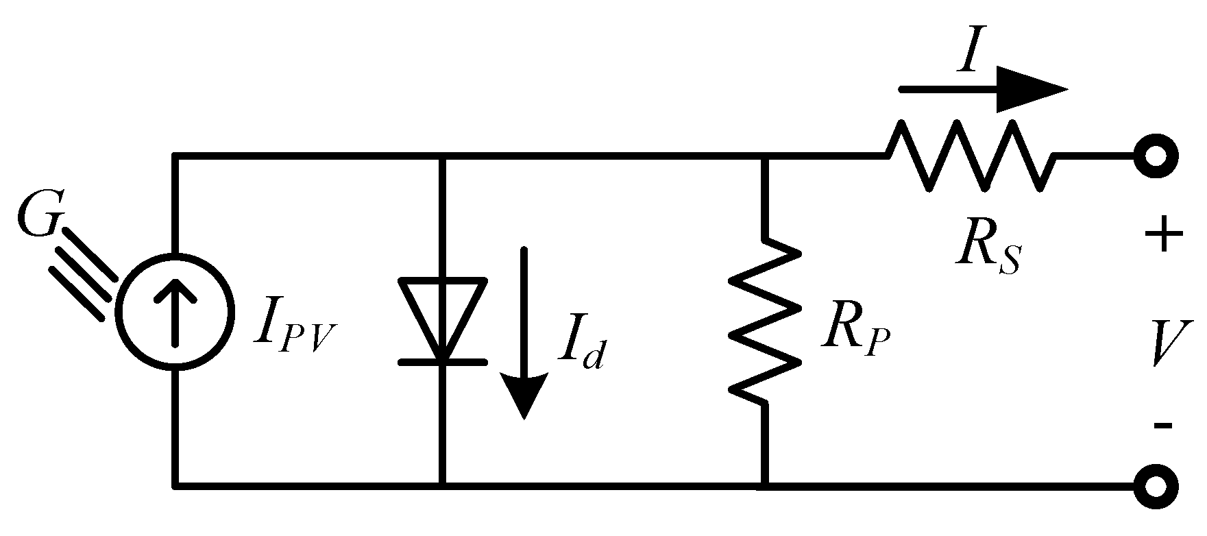
Figure 1 shows the equivalent circuit of a PV cell, where I_PV is the current that is generated by the incident light (G); I_d is the forward bias current of the diode; and, R_P and R_S are the intrinsic shunt resistance and internal series resistance of the cell, respectively. The relationship between the current (I) and voltage (V) of the solar cell can be expressed as

$$I=I_{PV}-I_0\left\{\exp \left[\frac{q\left(V+I{R}_S\right)}{nKT}\right]-1\right\}-\frac{V+I{R}_S}{R_P}$$

(1)

where I₀ is the diode reverse saturation current, q is the electron charge, K is Boltzmann constant, T (in Kelvin) is the temperature of the p-n junction, n is the diode ideality constant, and V + IR_s is the cross-voltage of the diode.

The five parameters (I_PV, I₀, R_S, R_P, and n) of the circuit model can be extracted from the datasheet-based information under three conditions (open circuit, short circuit, and maximum power point) [18]. As such, respectively substituting the parameters of the open circuit (V = V_OC, I = 0), short circuit (V = 0, I = I_SC), and maximum power point (V = V_mp, I = I_mp) conditions into Equation (1) yields:

$$0=I_{PV}-I_0\left[\exp \left(\frac{q{V}_{OC}}{nKT}\right)-1\right]-\frac{V_{OC}}{R_P}$$

(2)

$$I_{SC}=I_{PV}-I_0\left[\exp \left(\frac{q{I}_{SC}{R}_S}{nKT}\right)-1\right]-\frac{R_S{I}_{SC}}{R_P}$$

(3)

$$I_{MP}=I_{PV}-I_0\left\{\exp \left[\frac{q\left(V_{MP}+I_{MP}{R}_S\right)}{nKT}\right]-1\right\}-\frac{V_{MP}+R_S{I}_{MP}}{R_P}$$

(4)

where V_OC is the open circuit voltage, I_SC is the short circuit current, and V_mp and I_mp are voltage and current at the maximum power point, respectively. Typically, the shunt resistance R_P in practical devices is sufficiently large and it could be neglected. In addition, the value of R_S could also be obtained from the datasheet. Moreover, by exploiting Equations (2)–(4), other unknown parameters of the circuit model can be extracted.

2.2. Irradiance and Temperature Effects

The equations and parameters of the circuit model that is mentioned in the previous section are based on the standard test condition (STC), which consists of a cell temperature of 25 °C under 1000 W/m² solar irradiance with AM 1.5 spectral distribution. When considering the effect of temperature and irradiance changes, the light-generated current I_PV, which depends linearly on the solar irradiance and is influenced by the temperature, should be corrected by

$$I_{PV}=\left(I_{PV,STC}+K_I\Delta T\right)\frac{G}{G_{STC}}$$

(5)

where I_PV,STC is the light-generated current at STC, K_I is the temperature coefficient of the current, G is the irradiance level on the cell surface, G_STC is 1000 W/m², $\Delta T=T_{cell}-T_{STC}$, and T_cell and T_STC are the actual temperature of the solar cell and 25 °C, respectively. In addition, the diode reverse saturation current I₀ is strongly dependent on the temperature, and it can be modeled as [19]

$$I_0=\frac{I_{SC,STC}+K_I\Delta T}{\exp \left[\frac{q\left(V_{OC,STC}+K_V\Delta T\right)}{nKT}\right]-1}$$

(6)

where I_SC,STC and V_OC,STC are the short circuit current and open circuit voltage at STC, respectively, while K_I and K_V individually represent the temperature coefficients of the current and voltage.

To calculate the actual temperature of the solar cell T_cell, the normal operating cell temperature (NOCT) parameter that is provided by datasheet is usually adopted. NOCT is defined as the temperature reached by the open circuit cells in a module with an irradiance level of 800 W/m², ambient temperature of 20 °C, and wind speed of 1 m/s. Accordingly, T_cell could be calculated from NOCT by

$$T_{cell}=T_a+\frac{G}{800}\left(\mathrm{NOCT}-20\right)$$

(7)

where T_a is ambient temperature in Celsius, and G is the irradiance level on the cell surface.

2.3. Effects of PSCs and Bypass Diodes

To obtain the desired output voltage, solar cells are usually connected in series and/or parallel to form a PV module. As a result, Equation (1) can be modified to represent the relationship between the current and voltage of a PV module, and is modeled as

$$I=N_P\langle I_{PV}-I_0\left\{\exp \left[\frac{q\left(V+I{R}_S\right)}{nKT{N}_S}\right]-1\right\}\rangle -\frac{V+I{R}_S}{R_P}$$

(8)

where N_S and N_P are the number of cells connected in series and parallel, respectively. Similarly, practical PV arrays are composed of several connected PV modules. Usually, blocking and bypass diodes are used to protect PV modules from current reverse flow and hot-spot issues, respectively. However, the P-V curves of the PV arrays under PSCs with bypass diodes might exhibit multiple LMPPs, which increases the complexity of the system’s MPPT [6].

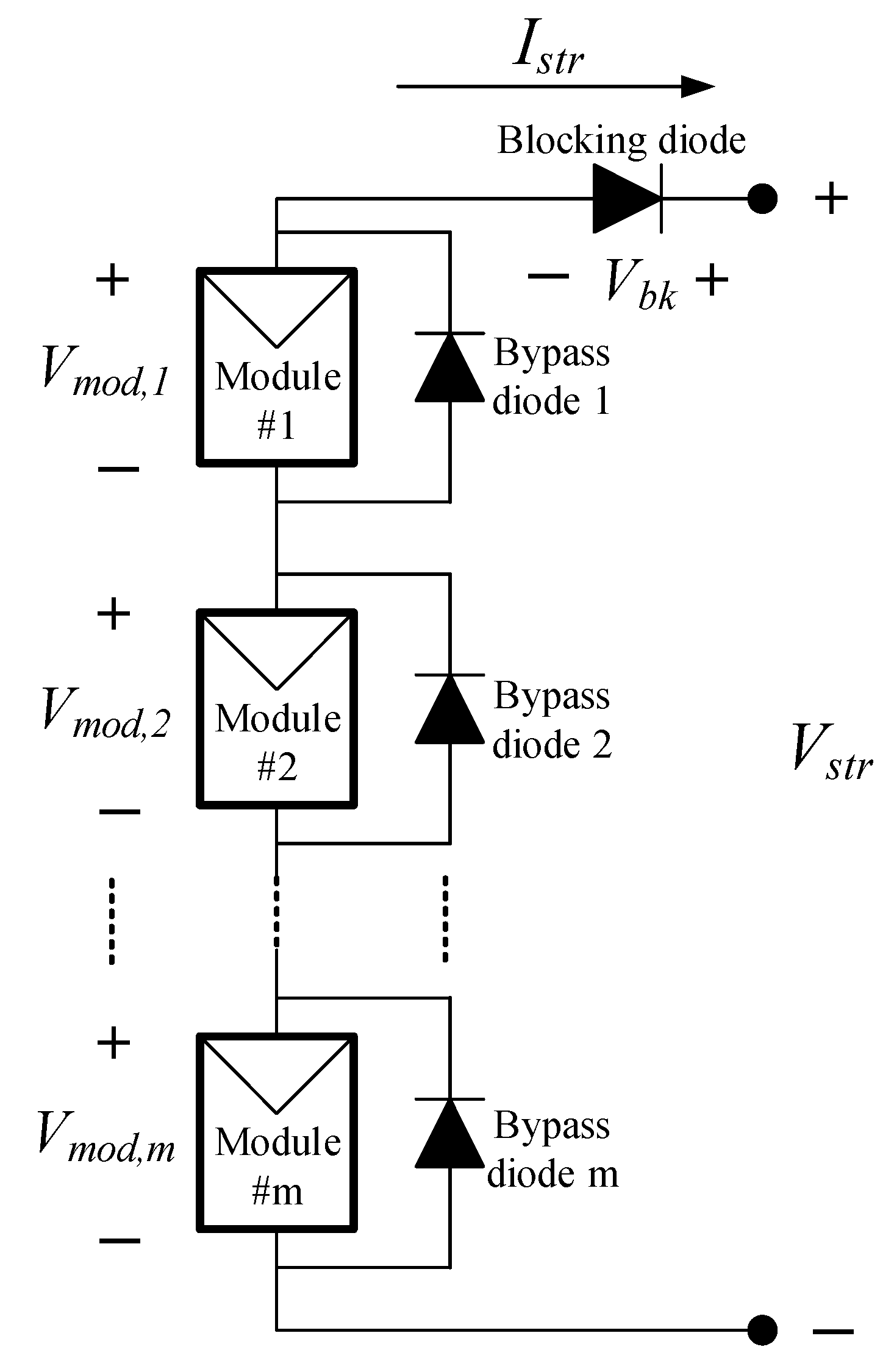
In order to more comprehensively model the I-V relationship of a series-connected PV array with bypass and blocking diodes, a PV string composed of m modules is illustrated in Figure 2. Each module of the string is protected by a bypass diode; in addition, one blocking diode is connected at the end of the string. Here, the voltage of the PV string V_str could be calculated by summing the individual module voltage V_mod,i and the voltage drop of the blocking diode V_bk. In addition, the calculation of V_mod,i depends on the string operating current I_str and the short circuit current I_SC,i (approximately equal to the photocurrent of the module) of each module i. When I_str is equal to or smaller than I_SC,i, the positive module voltage V_mod,i could be calculated while using the Lambert W function [20]; in contrast, when I_str is larger than I_SC,i, the bypass diode conducts, and V_mod,i is clipped to a small negative voltage equal to the forward bias voltage of the bypass diode. As such, the module operates at its short circuit current I_SC,i, and therefore the bypass diode carries the difference of the string current I_str and I_SC,i. Consequently, the relationship between the PV string voltage V_str and current I_str could be modeled by

$$V_{str}={\displaystyle \sum }_{i=1}^m{V}_{mod,i}+V_{bk}$$

(9)

$$V_{mod,i}=\{\begin{array}{l}{R}_P·\left(I_{PV}+I_0\right)-\left(R_S+R_P\right)·I_{str}-a·W\left\{\frac{R_P{I}_0}{a}\exp \left[\frac{R_P\left(I_{PV}+I_0-I_{str}\right)}{a}\right]\right\},I_{str}\le I_{SC,i}\hfill \\ -\frac{n_{bp}KT}{q}·\ln \left(\frac{I_{str}-I_{SC,i}}{I_{0,bp}}+1\right),I_{str}>I_{SC,i}\hfill \end{array}$$

(10)

$$V_{bk}=-\frac{n_{bk}KT}{q}·\ln \left(\frac{I_{str}}{I_{0,bk}}+1\right)$$

(11)

where W{x} denotes the Lambert W function, which is the inverse of the equation $W·e^W=x$, $a=nKT/q$, n_bp and n_bk, respectively, represent the ideality constants of the bypass and blocking diodes, and I_0,bp and I_0,bk correspond to the reverse saturation current of the bypass and blocking diodes.

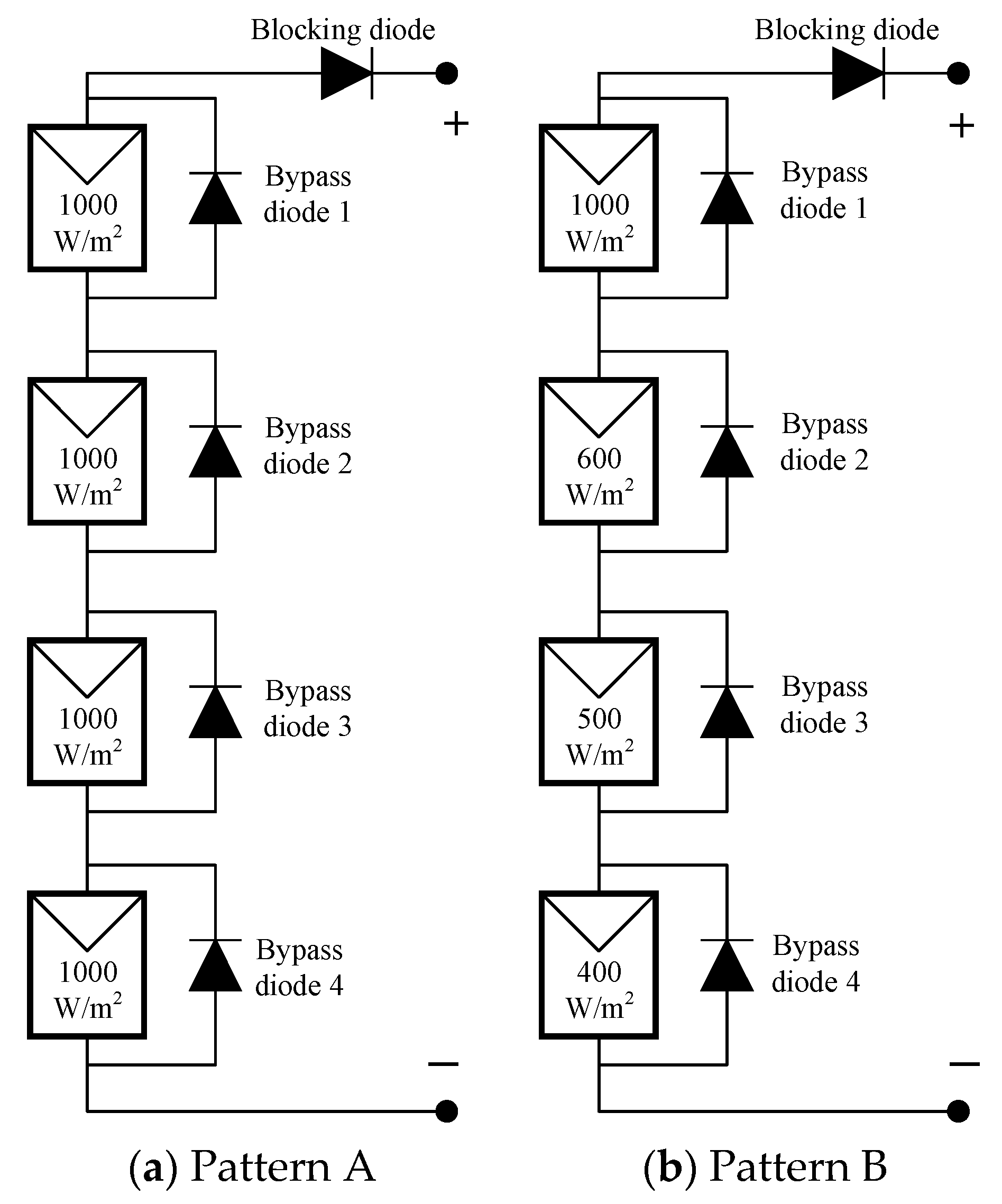
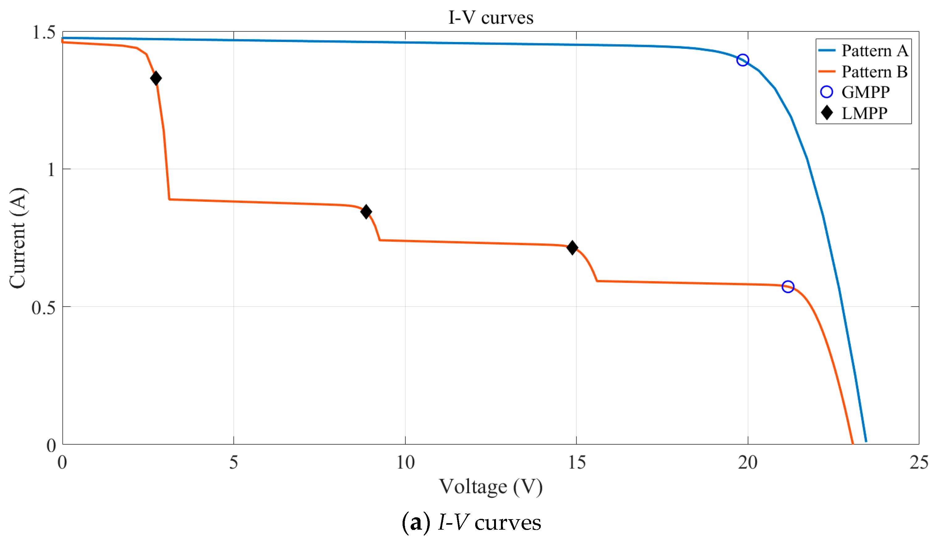
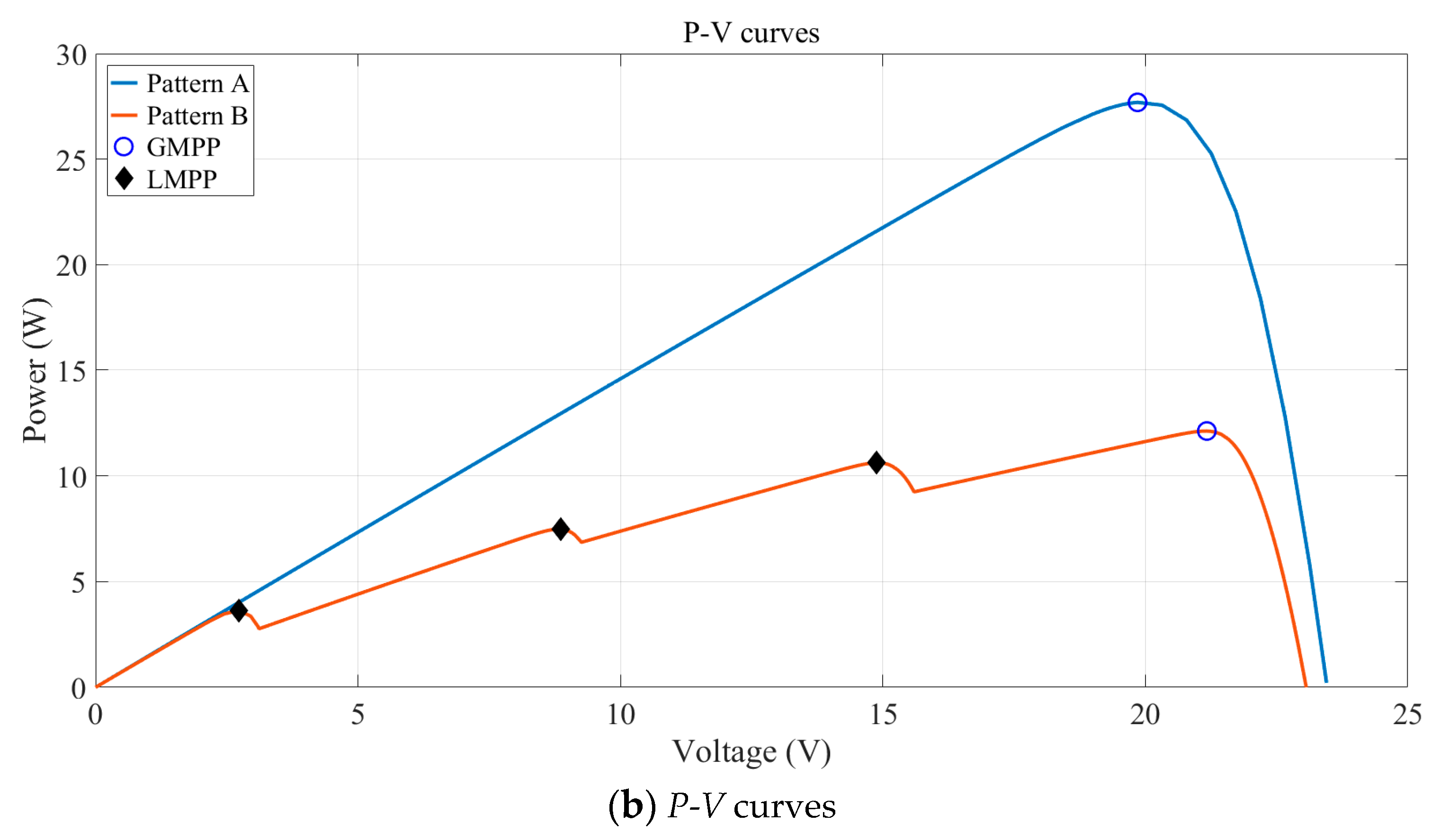
Under PSCs, I_SC,i in Equation (10), which is approximately equal to the photocurrent and directly proportional to the irradiance of its corresponding module, might be different for all the modules of a PV string. This could cause steps in the I-V curves and multiple LMPPs in the P-V curves. Figure 3 illustrates a PV array, which comprises four PV modules in series with blocking and bypass diodes, under both uniform irradiance (Pattern A) and PSCs (Pattern B). As demonstrated in Figure 4, with four series-connected modules each under a different irradiance level, both the interval number and LMPP number of the array’s I-V and P-V curves are 4. As such, the resulting P-V curve will become more complex, resulting in numerous peaks in one array with long strings. Under such conditions, conventional MPPT methods can easily fail to identify the GMPP among the LMPPs and become trapped at a local peak, which might significantly reduce the output power of the PV modules. In addition, the irradiance level will likely change rapidly, thereby causing variations in the curve pattern and the location of the GMPP. Accordingly, to extract the maximum power output of the system under PSCs, the adopted MPPT algorithm should be able to quickly and accurately identify the GMPP among the LMPPs.

2.4. FA for MPPT under PSCs

The FA has been verified as an effective optimization technique that is based on swarm intelligence. The search pattern of the FA is determined by the attractions among fireflies, whereby a dim firefly moves toward a brighter firefly. To implement the FA for solar MPPT application, the locations of the fireflies are usually defined as different operating points along the P-V curve of a PV array. Specifically, the brightness of each firefly is taken as the generated power of the PV array, and so it corresponds to the position of the particular firefly. Consequently, several operating points of the PV array are initially distributed along the P-V curve and are then adjusted based on the FA algorithm, which measures the voltage and current, and then calculates the output power of the operating points to identify the MPPs. It has been confirmed that the FA implemented for a PV system’s MPPT under PSCs can accurately track the GMPP with simple computational processes, fast convergence, and lower turbulence in PV power [6,13].

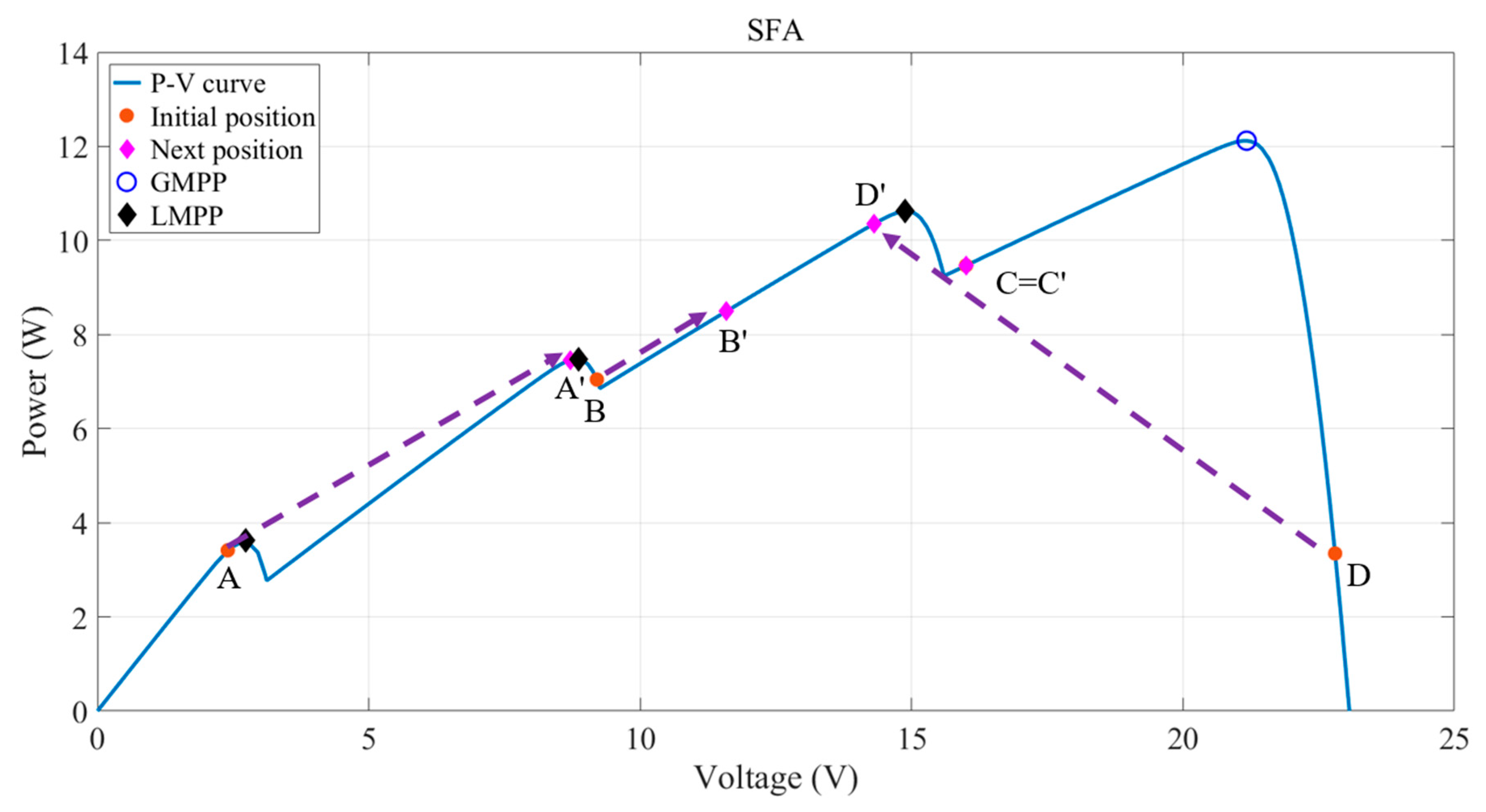
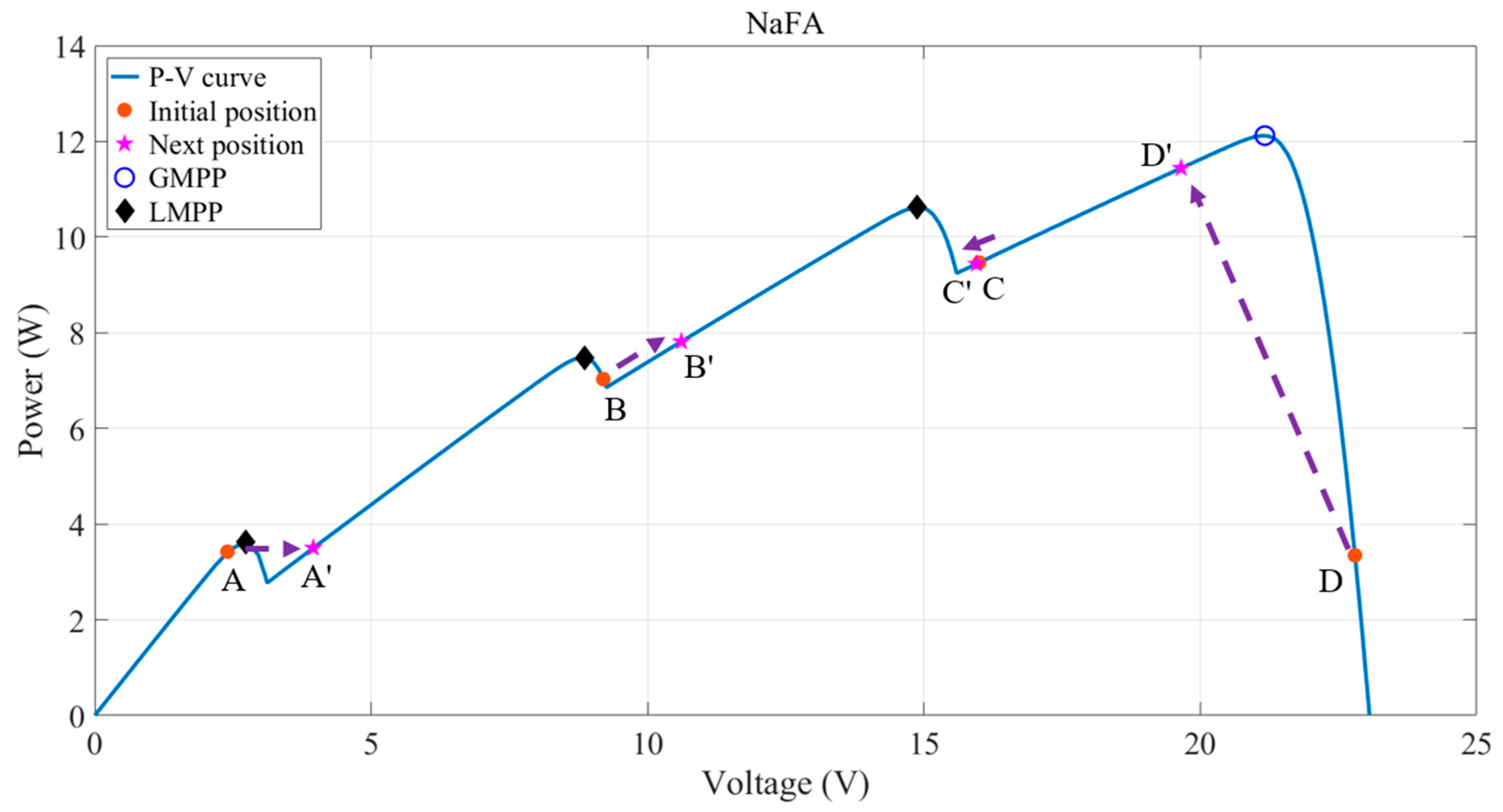
Nevertheless, improvements to the tracking speed of the FA can be made for solar MPPT applications, especially under rapidly-changing environmental conditions. The SFA algorithm, which is modified from the FA, was proposed to improve the tracking speed [21]. However, as aforementioned, the simplification of the convergence process has the tradeoff of decreased tracking accuracy and more frequent trapping in LMPPs. Figure 5 illustrates the adjustment of the operating points in the P-V curve of a PV array under PSCs with the SFA. It can be seen that when the positions of the four initial fireflies (A to D) are adjusted to new positions (A′ to D′) after the first iteration, firefly D might be attracted by the three other fireflies and leave the actual GMPP interval and move to the local-peak interval. In this manner, too many attractions may cause the fireflies to become trapped at the LMPPs or produce oscillations during the search process. In response, the NaFA was proposed to overcome these problems, in which each firefly is attracted by other brighter fireflies selected from a predefined neighborhood rather than those from the entire population [16]. To illustrate this concept, Figure 6 shows that firefly D is only attracted by neighbor C, thereby preventing over-movement. Compared with the SFA, the NaFA can indeed improve the tracking accuracy, but with slower convergence speed. From trial and error experiments, we found that one iteration of the NaFA is sufficient to prevent LMPP trapping in most cases. Consequently, to simultaneously exploit the advantages of the NaFA’s high accuracy and the SFA’s fast convergence, this work proposes a fusion algorithm that integrates the NaFA and SFA for MPPT.

2.5. Processes of the Proposed Algorithm

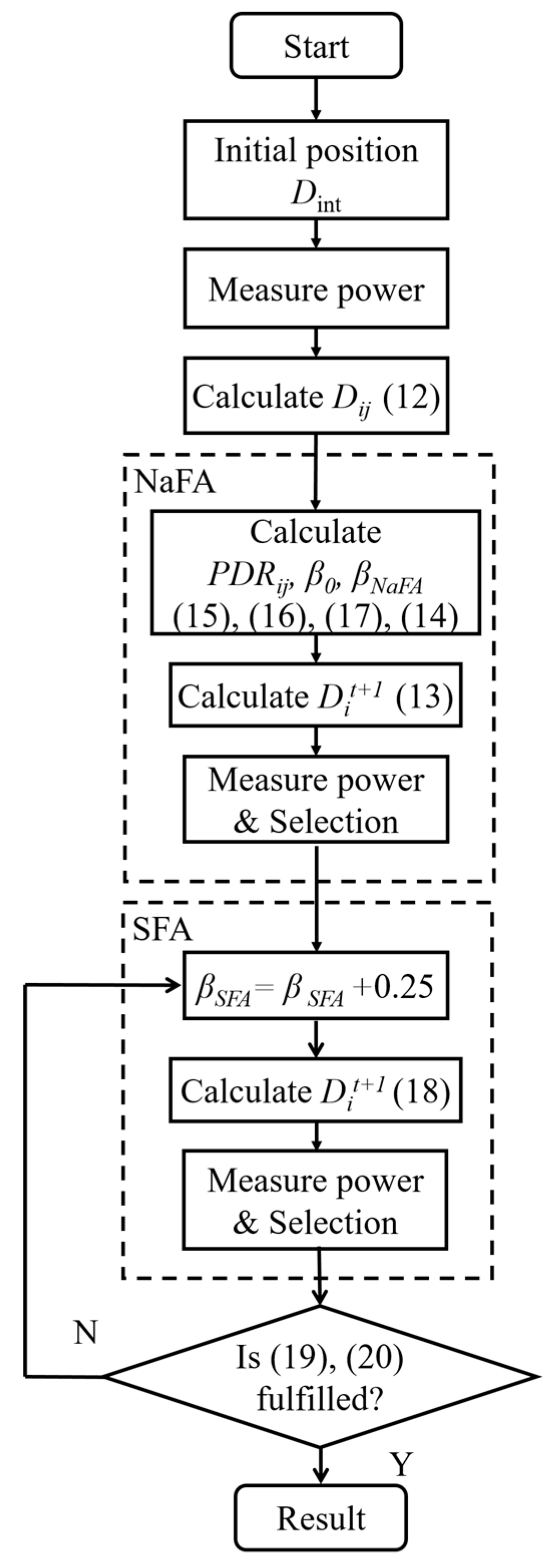
In this study, the proposed modified firefly algorithm (MFA) integrates the NaFA and SFA algorithms for solar MPPT under PSCs. A boost power converter is used as the interface to feed the output power of a PV array to a load. The operating points of the PV array’s P-V curve are controlled by adjusting the pulse-width-modulation (PWM) signal of the power converter. Accordingly, the positions of the fireflies are defined as the on/off duty cycle of the PWM signals in this study. As with the FA, the brightness of each firefly is taken as the generated power of the PV array, and so it corresponds to the position of the particular firefly. The processing flow of the proposed MFA algorithm is presented in Figure 7. As seen, the MFA is composed of two major processes, namely the modified NaFA and SFA. In the modified NaFA process, the fireflies are initially positioned and uniformly distributed in four duty-cycle points (D_ini = 0.05, 0.333, 0.616, and 0.90).

The corresponding voltage and current of each firefly at its different position are then measured for power calculation. In addition, the distance D_ij is calculated by

$$D_{ij}=D_j-D_i;i,j=1~4,i\ne j$$

(12)

where D_i and D_j are the positions of fireflies i and j. In a NaFA, fireflies are attracted only by brighter neighborhoods, which could reduce the phenomenon of oscillations, which easily leads to trapping at LMPPs with the conventional FA. The movement of a firefly i, which is attracted by a brighter firefly j, is given by

$$D_i^{t+1}=D_i^t+{\beta }_{NaFA}·D_{ij}+\alpha \epsilon$$

(13)

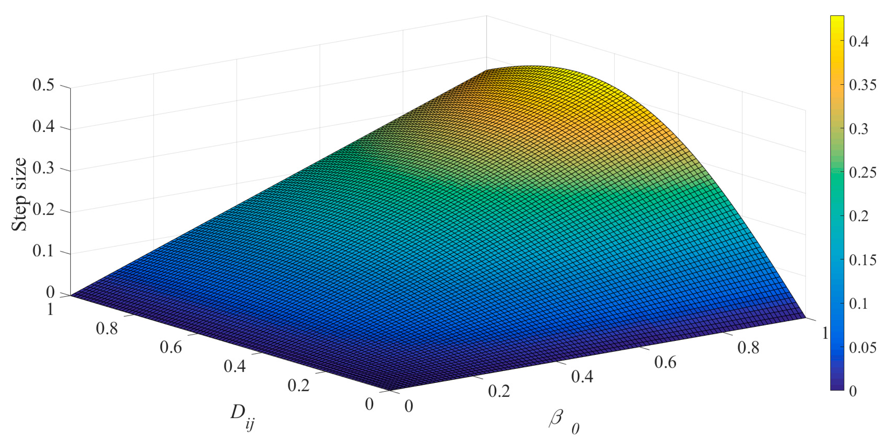
where D_i^t and D_i^t+1 are the current and next positions of firefly i, respectively, β_NaFA is the degree of attractiveness, D_ij is the distance between fireflies i and j, α represents a random coefficient that decreases with iterations by a reduction constant θ, and ε denotes a random number. Here, β_NaFA∙D_ij is the step size of the movement, which is directly proportional to β_NaFA and D_ij. As a result, with the same degree of attractiveness, a larger distance between two fireflies will lead to a larger movement step size and faster convergence speed. The degree of attractiveness β_NaFA is derived by [12]

$${\beta }_{NaFA}={\beta }_0\left[\exp {\left(-\gamma \left|D_{ij}\right|\right)}^2\right]$$

(14)

where β₀ denotes the initial attractiveness and γ is the light absorption coefficient. It is observed that a shorter distance D_ij leads to higher attractiveness β_NaFA; and contrastively, a larger distance leads to lower attractiveness. Figure 8 shows the relationship between the step size (duty cycle of the converter), distance D_ij, and initial attractiveness β₀.

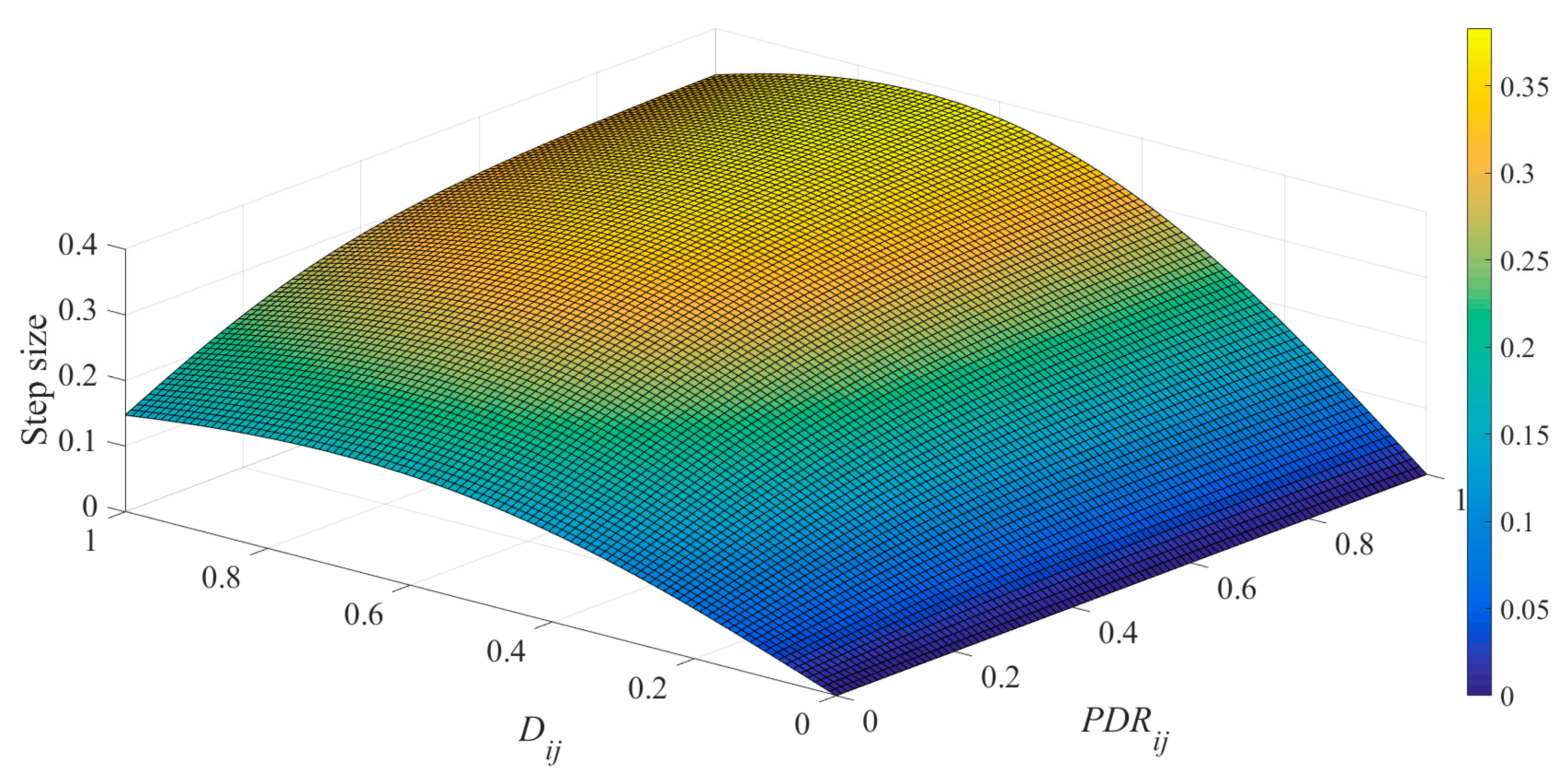
The initial attractiveness β₀ of the conventional NaFA is set as a constant, which means that the brightness of fireflies does not change during the entire moving process. Be that as it may, the output power (brightness) of fireflies at different positions in the P-V curve might be different. Accordingly, the initial attractiveness in the NaFA should be adapted to solar application. In this study, β₀ is set as a dynamic parameter affected by the power difference ratio PDR_ij. The PDR_ij of a firefly i and a brighter firefly j is defined and calculated by

$$PD{R}_{ij}=1-\frac{P_i}{P_j}$$

(15)

where P_i and P_j are the output power of fireflies i and j, respectively. Since P_j is larger than P_i, PDR_ij will range between 0 and 1. In this manner, a larger PDR_ij means a larger power difference ratio between two fireflies, which should lead to larger initial attractiveness β₀. The relationship between PDR_ij and β₀ is designed to be transferred by a hyperbolic tangent sigmoid transfer function. Furthermore, setting the range of β₀ could be used for adjusting tracking accuracy and speed optimization [16]. As a result, two parameters are used for β₀ to range from a to b. Consequently, the calculation of β₀ could be expressed by

$${\beta }_{0,sig}=\frac{2}{1+\exp \left(-5\times PD{R}_{ij}\right)}-1$$

(16)

$${\beta }_0={\beta }_{0,sig}\times \left(b-a\right)+a$$

(17)

where β_0,sig is a parameter transferred from PDR_ij by the hyperbolic tangent sigmoid transfer function.

Since, in this study, the fireflies are initially positioned in four duty cycle points and uniformly distributed from 0.05 to 0.90, the initial distance D_ij between each pair of fireflies is 0.283. From trial and error experiments of different step sizes, the optimized range setting of β₀ is from 0.4 to 0.9. Figure 9 shows the relationship between step size, distance D_ij, and power difference ratio PDR_ij of the proposed NaFA process. As illustrated in Figure 7, the next position D_i^t+1 of a firefly i is then calculated. Since D_i^t+1 is affected by all other brighter fireflies, it is sequentially calculated using Equation (13) with each brighter firefly j. The corresponding output power of the firefly at its new position is then measured. After that, a total of eight fireflies from the initial and second generations are sorted. Of the eight fireflies, the three with the largest output power are selected for the next SFA process.

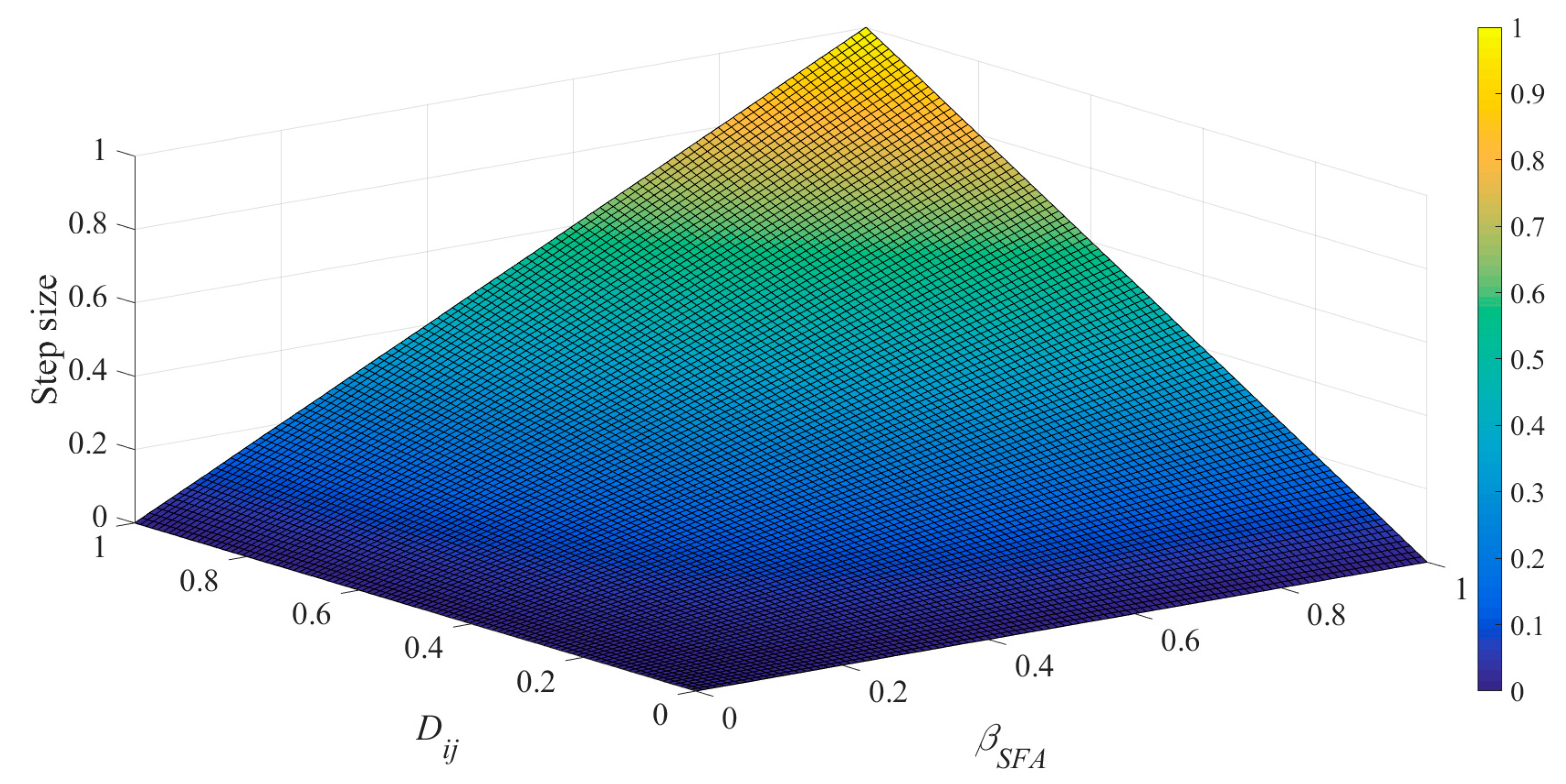
The modified SFA process is executed after the NaFA process. In order to accelerate the convergence speed of the conventional FA, the degree of attractiveness β_SFA of the conventional SFA is regularly increased by 0.25 after each iteration [16]. With this setting, a lower β_SFA in the initial iterations might improve the accuracy of searching for LMPPs; meanwhile, a higher β_SFA in the following iterations will accelerate the searching speed. In addition, in the SFA, parameters α, ε, and γ are omitted for simplification. Consequently, the simplified calculation of the movement of a firefly i attracted by a brighter firefly j is given by

$$D_i^{t+1}=D_i^t+{\beta }_{SFA}·D_{ij}$$

(18)

where D_i^t and D_i^t+1 are the current and next positions of firefly i, respectively, and D_ij is the distance between fireflies i and j. As a result, the step size of movement β_SFA∙D_ij and the searching speed will be directly proportional to β_SFA and D_ij, as illustrated in Figure 10. In this study, the movement calculation of the modified SFA is the same as that in the conventional SFA; however, the number of fireflies is reduced from three in first iteration to two in the following iterations. During each iteration, the output power of each firefly is measured for the selection process until the convergence judgment is satisfied.

3. Simulation

3.1. Simulation Setup

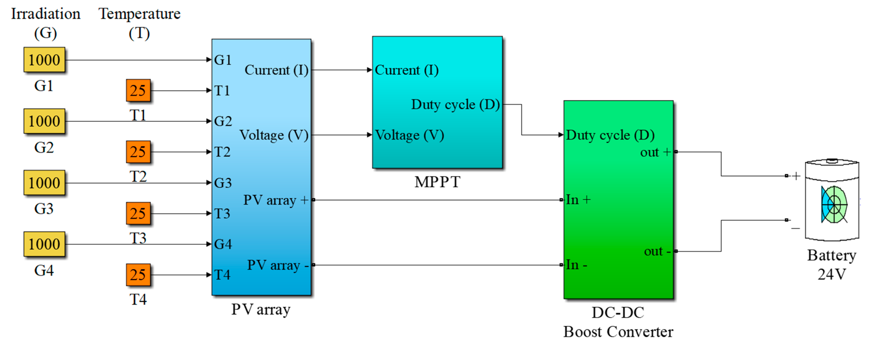
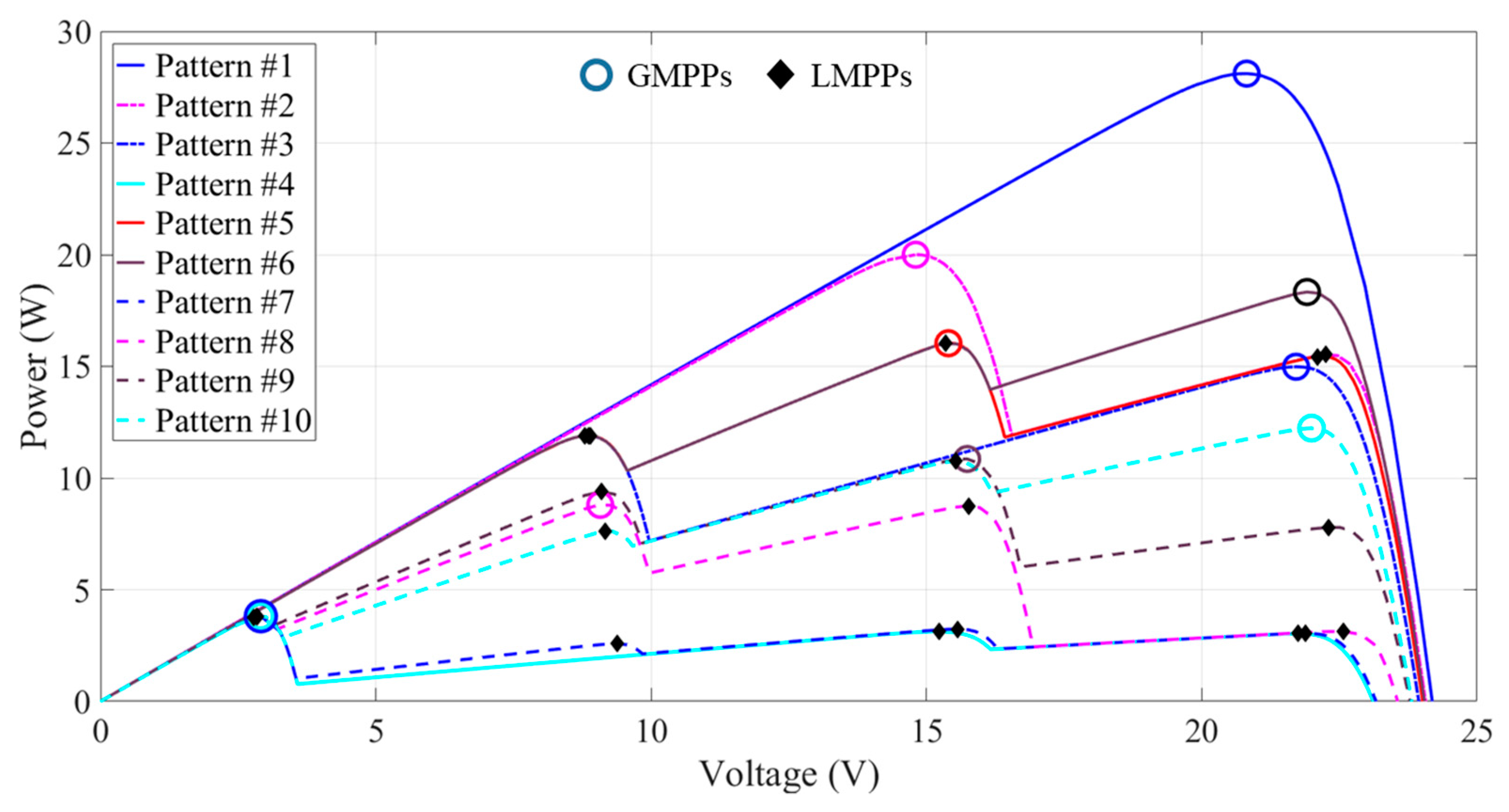
The proposed algorithm was first simulated with the Simulink toolbox of MATLAB R2016a software, the system blocks for which are shown in Figure 11. The PV array was composed of four series-connected modules (Modules #1–#4), with their parameters being given in

Table 1. Parameters of the experimental modules.

Variables	Spec.
VOC	6.04 V
ISC	1.43 A
Vmp	5.13 V
Imp	1.37 A
Pmp	7.02 W
KV	−0.522%/°C
KI	0.144%/°C
NOCT	45 °C
RS	27.2 mΩ
RS (bypass diode)	12 mΩ
nbp (bypass diode)	1.2

. The temperature of the modules (T1–T4) was controlled at 25 °C. The irradiation setups (G1–G4) for each module could be individually programmed to generate different PSCs.

Table 2. Irradiance setups of the 10 evaluation patterns (W/m²).

Irradiance Setup	LMPPs	Module #1	Module #2	Module #3	Module #4
Pattern #1	1	1000	1000	1000	1000
Pattern #2	2	1000	1000	1000	500
Pattern #3	2	1000	1000	500	500
Pattern #4	3	1000	150	150	100
Pattern #5	3	1000	750	750	500
Pattern #6	3	1000	1000	750	500
Pattern #7	4	1000	200	150	100
Pattern #8	4	1000	700	400	100
Pattern #9	4	1000	750	500	250
Pattern #10	4	1000	600	500	400

lists the 10 different PSCs (Patterns #1–#10), the purpose of which was to simulate patterns that have 1–4 LMPPs, with their respective GMPP located at different intervals. Figure 12 illustrates the P-V curves of the PV array under the 10 different patterns and their corresponding GMPPs (#1–#10). Five different MPPT algorithms, FPA, FA, NaFA, SFA, and the proposed MFA were implemented in the MPPT block to compare and evaluate tracking accuracy and speed. The operating voltage and current of the PV array were measured as input data of the MPPT algorithms. A DC-DC boost converter controlled by a PWM signal was used as the interface to feed the output power of the PV array to a 24 V battery load. The duty cycle (D) of the PWM signal is adjusted by the MPPT algorithms to change the operating point of the PV array. All of the simulations were conducted using a computer with a standard Intel i7 Processor and 16 GB RAM.

Simulations were conducted under the same conditions for the five MPPT algorithms and all of the experiments were performed with the same initial position of the operating points, as indicated in Section 2.5. The convergence judgment criteria, according to Equations (19) and (20), were the same for all the algorithms.

$$P_{i\_\min }/P_{j\_\max }\ge 98.75\%$$

(19)

$$\left|D_{j\_\max }-D_{i\_\min }\right|<0.05$$

(20)

where P_{i_min} and P_{j_max} are the minimum and maximum output power of the operating points, while D_{i_min} and D_{j_max} are their respective positions that are represented as the duty cycle. Both criteria must be satisfied to be judged as converged. As soon as both criteria are satisfied, convergence is confirmed and the operating point with P_{j_max} is considered as the estimated MPP of the algorithm. The difference between the power of the estimated MPP (P_{MPP_est}) and the power of the actual MPP (P_{MPP_true}) is considered as the error (ERR), which is expressed as

$$ERR(\%)=1-\frac{P_{MPP\_est}}{P_{MPP\_true}}\times 100\%$$

(21)

The MPPT performance is assessed in terms of the percentage of energy generated from the PV array during the simulation period, which is calculated by [19]

$${\eta }_{mppt}(\%)=\frac{E_{mppt}}{E_{MPP\_true}}=\frac{\int P_{mppt}dt}{\int P_{MPP\_true}dt}\times 100\%$$

(22)

where η_mppt is the tracking efficiency of the MPPT algorithm, and E_mppt is the energy extracted by the algorithm, which is calculated by the integral of the module output power P_mppt over time; meanwhile, E_{MPP_true} and P_{MPP_true} denote the energy and power of the actual MPP, respectively. The simulation was iterated 100 times, with the averaged ERR and η_mppt of each algorithm, corresponding to tracking accuracy and efficiency, being used for comparison. In addition, the number of measured operating points during the tracking process was counted as the sampling times. The total sampling times and execution time needed before convergence for each algorithm were averaged for tracking speed comparison.

Table 3. Parameter settings of the flower pollination algorithm (FPA), firefly algorithm (FA), NaFA, SFA, and the proposed MFA.

FPA [11]	FA [16]	NaFA [15]	SFA [21]	Proposed MFA
P = 0.8	α = 0.012	α = 0.012	β = [0.3 0.55 0.8 1]	a = 0.4
γ = 1.5	β = 0.5	β = 0.5	-	b = 0.9
-	γ = 1	γ = 1	-	α = 0.012
-	θ = 0.97	θ = 0.97	-	β = [0.3~1]
-	-	-	-	γ = 1
-	-	-	-	θ = 0.97

lists the parameter settings of the five MPPT algorithms for evaluation. The settings of the four conventional algorithms are based on the literature. Since the experimental PV array was composed of four series-connected modules, the maximum interval number of the array’s P-V curve under PSCs was four. In order to select the proper initial population number for the experiments, a preliminary evaluation was conducted. The initial population number was evaluated from three to six for all algorithms.

Table 4. Simulation results of the FPA with different population numbers under the 10 patterns.

Population #	Average Iterations	Average Sampling Times	Average Error (%)
3	4.79	14.36	4.89
4	5.79	23.16	2.11
5	5.93	29.64	2.27
6	6.34	38.03	2.46

,

Table 5. Simulation results of the FA with different population numbers under the 10 patterns.

Population #	Average Iterations	Average Sampling Times	Average Error (%)
3	6.97	20.92	3.27
4	6.11	24.45	2.72
5	5.7	28.49	1.71
6	5.46	32.74	2.19

,

Table 6. Simulation results of the NaFA with different population numbers under the 10 patterns.

Population #	Average Iterations	Average Sampling Times	Average Error (%)
3	11.93	35.80	13.33
4	13.57	54.28	13.46
5	18.71	93.53	13.44
6	20.64	123.85	13.41

,

Table 7. Simulation results of the SFA with different population numbers under the 10 patterns.

Population #	Average Iterations	Average Sampling Times	Average Error (%)
3	3.9	11.7	8.02
4	3.5	14	5.28
5	3.4	17	7.22
6	3.2	19.2	3.92

and

Table 8. Simulation results of the MFA with different population numbers under the 10 patterns.

Population #	Average Iterations	Average Sampling Times	Average Error (%)
3	3.78	9.38	5.32
4	3.83	12.21	1.65
5	3.82	15.82	1.98
6	4.55	21.82	1.66

list the averaged iterations, sampling times, and errors under the 10 irradiation patterns using the five different algorithms. It was observed that sampling time is proportional to population number for all algorithms, while number of iterations and errors exhibit different trends for different algorithms. Considering the fewer sampling times and reasonable tracking accuracy for most algorithms, a population number of 4 was chosen for further evaluation experiments.

3.2. Simulation Results

Table 9. Simulation results of the tracking speed, accuracy and efficiency.

Patterns	Algorithms	Sampling Times		Time (ms)		Error (%)		Efficiency (%)
		Average	SD	Average	SD	Average	SD	Average	SD
Pattern #1	FPA	19.2	5.628	3.05	0.0011	10.264	0.067	85.23	0.056
	FA	22.92	1.785	1.28	0.0002	0.788	0.002	95.78	0.002
	NaFA	32.52	1.673	1.84	0.0002	0.802	0.003	94.53	0.002
	SFA	12	0.001	0.73	0.0001	0.008	0.001	96.92	0.001
	MFA	11	0.001	0.88	0.0003	0.430	0.001	96.24	0.07
Pattern #2	FPA	20.04	8.327	4.43	0.0021	2.352	0.035	94.13	0.027
	FA	12.28	1.026	0.92	0.0001	0.042	0.001	97.62	0.001
	NaFA	28.16	1.963	2.07	0.0002	0.019	0.001	95.9	0.001
	SFA	12	0.001	0.93	0.0002	0.042	0.001	97.7	0.001
	MFA	11.44	0.833	1.15	0.0003	0.142	0.001	96.88	0.108
Pattern #3	FPA	16.64	5.818	3.12	0.0010	1.229	0.002	96.08	0.021
	FA	25.48	2.1	1.62	0.0002	1.203	0.001	96.28	0.003
	NaFA	40.28	2.621	1.90	0.0010	0.260	0.001	92.71	0.009
	SFA	12	0.001	0.83	0.0001	6.020	0.001	92.65	0.001
	MFA	15	0.001	1.46	0.0002	0.552	0.001	96.37	0.009
Pattern #4	FPA	32.72	17.555	7.25	0.0038	2.232	0.033	91.27	0.032
	FA	36.68	6.072	2.58	0.0004	0.164	0.001	88	0.002
	NaFA	104	0.001	7.09	0.0004	12.299	0.001	76.98	0.018
	SFA	16	0.001	1.23	0.0002	12.299	0.001	83.83	0.001
	MFA	15	0.001	1.64	0.0004	4.076	0.001	91.85	0.04
Pattern #5	FPA	23.52	14.182	5.16	0.0029	0.960	0.015	95.59	0.017
	FA	15.32	1.510	1.10	0.0002	0.255	0.003	97.72	0.003
	NaFA	29	2	2.00	0.0002	0.044	0.001	96.54	0.001
	SFA	12	0.001	0.9	0.0001	1.059	0.001	97.21	0.001
	MFA	12.18	1.209	1.55	0.0005	0.836	0.015	96.48	1.729
Pattern #6	FPA	16.36	5.275	3.41	0.0017	1.380	0.027	94.45	2.334
	FA	24.72	2.502	1.51	0.0003	12.265	0.007	85.91	0.751
	NaFA	34.88	2.279	2.16	0.0003	3.026	0.004	93.36	0.416
	SFA	12	0.001	0.78	0.0001	8.086	0.001	90.18	0.001
	MFA	13	0.001	1.19	0.0003	0.694	0.001	96.66	0.082
Pattern #7	FPA	38.32	21.251	7.31	0.0036	2.194	0.022	92.09	0.035
	FA	36.68	5.212	2.69	0.0005	0.181	0.001	89.75	0.002
	NaFA	104	0.001	7.03	0.0002	12.286	0.001	83.46	0.001
	SFA	16	0.001	1.25	0.0002	12.286	0.001	84.71	0.001
	MFA	15	0.001	1.63	0.0004	4.478	0.004	92.04	0.51
Pattern #8	FPA	25.88	18	5.70	0.0038	0.016	0.001	96.48	0.007
	FA	29.12	3.983	1.93	0.0003	0.022	0.001	95.37	0.006
	NaFA	104	0.001	6.34	0.0004	0.031	0.001	92.7	0.004
	SFA	16	0.001	1.09	0.0002	0.031	0.001	97.18	0.001
	MFA	13	0.001	1.20	0.0003	0.031	0.001	96.99	0.056
Pattern #9	FPA	20.12	8.209	3.69	0.0014	0.367	0.005	95.99	0.011
	FA	17.92	2.308	1.19	0.0002	0.369	0.004	97.05	0.005
	NaFA	29.52	3.05	1.94	0.0004	0.060	0.001	95.51	0.001
	SFA	16	0.001	1.1	0.0001	0.099	0.001	97.48	0.001
	MFA	13	0.001	1.23	0.0004	0.121	0.001	97.41	0.018
Pattern #10	FPA	16.24	4.852	3.44	0.0011	1.957	0.028	94.92	0.022
	FA	24.24	3.355	1.62	0.0003	12.03	0.007	85.99	0.007
	NaFA	35.76	2.351	2.38	0.0003	3.041	0.004	93.28	0.004
	SFA	16	0.001	1.11	0.0002	13.00	0.001	85.52	0.001
	MFA	13	0.001	1.28	0.0003	1.13	0.001	96.26	0.089

summarizes the simulation results of the sampling times, execution times, errors and efficiencies of the five MPPT algorithms under the 10 PSC patterns. It is observed that the SFA and MFA require fewer sampling times and shorter execution times than the other algorithms under most patterns. However, the error of the SFA was usually larger than the other algorithms under Patterns #3–#7, and #10. In addition, the proposed MFA has the highest tracking efficiency under Patterns #3, #4, #6, and #10, thereby verifying that it can provide faster tracking speed with good accuracy and efficiency. On the other hand, due to the step size of the FPA being associated with Levy flight, the SD of its sampling times, execution time, and error are larger than the other algorithms. In addition, the sampling times and execution time of the NaFA reach maximum values under Patterns #4, #7, and #8, which is due to it failing to satisfy the convergence criteria during the simulation period.

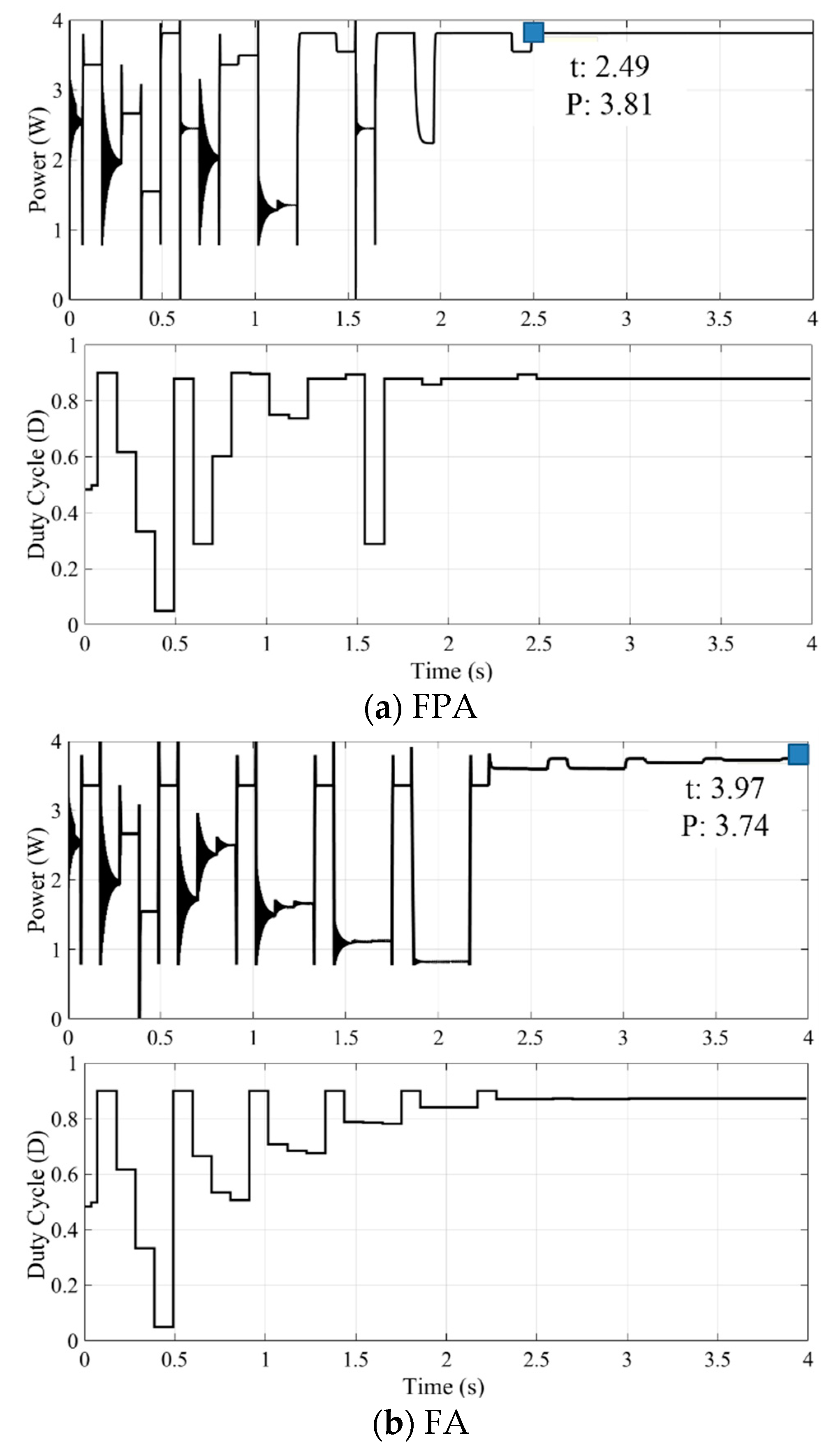
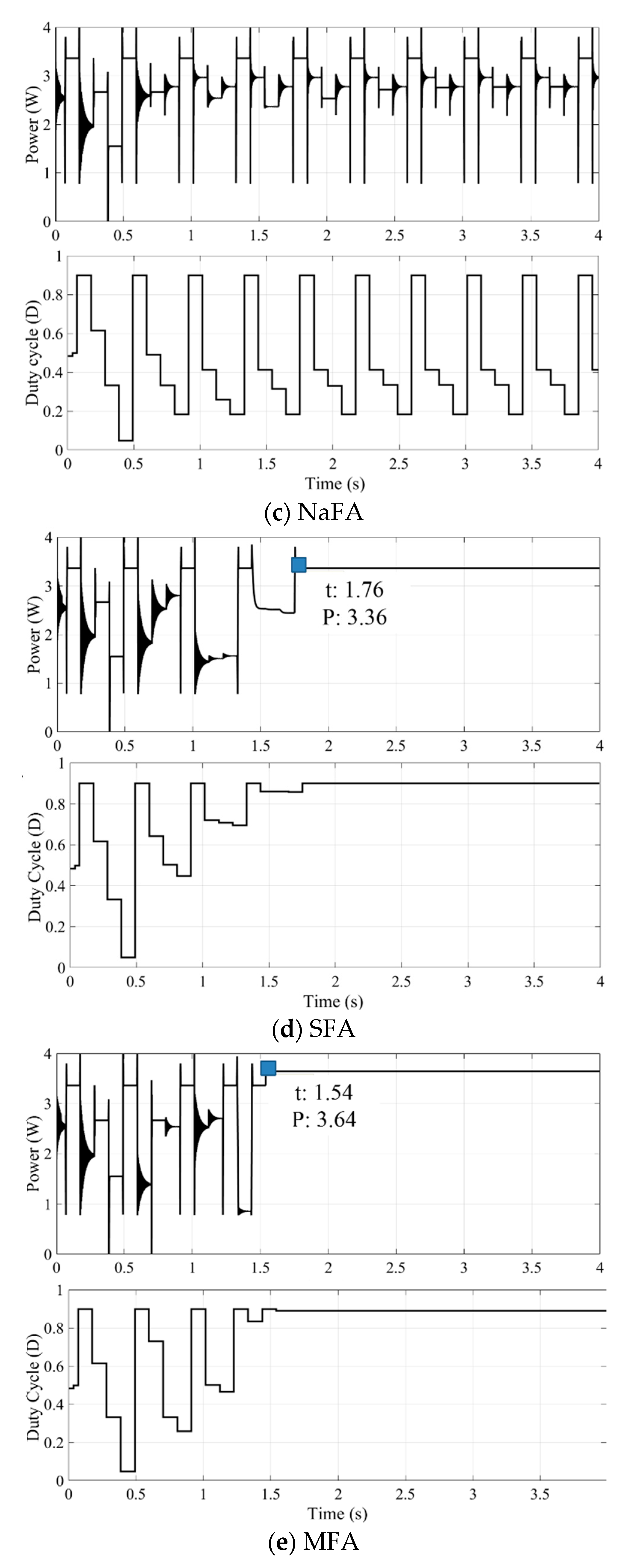
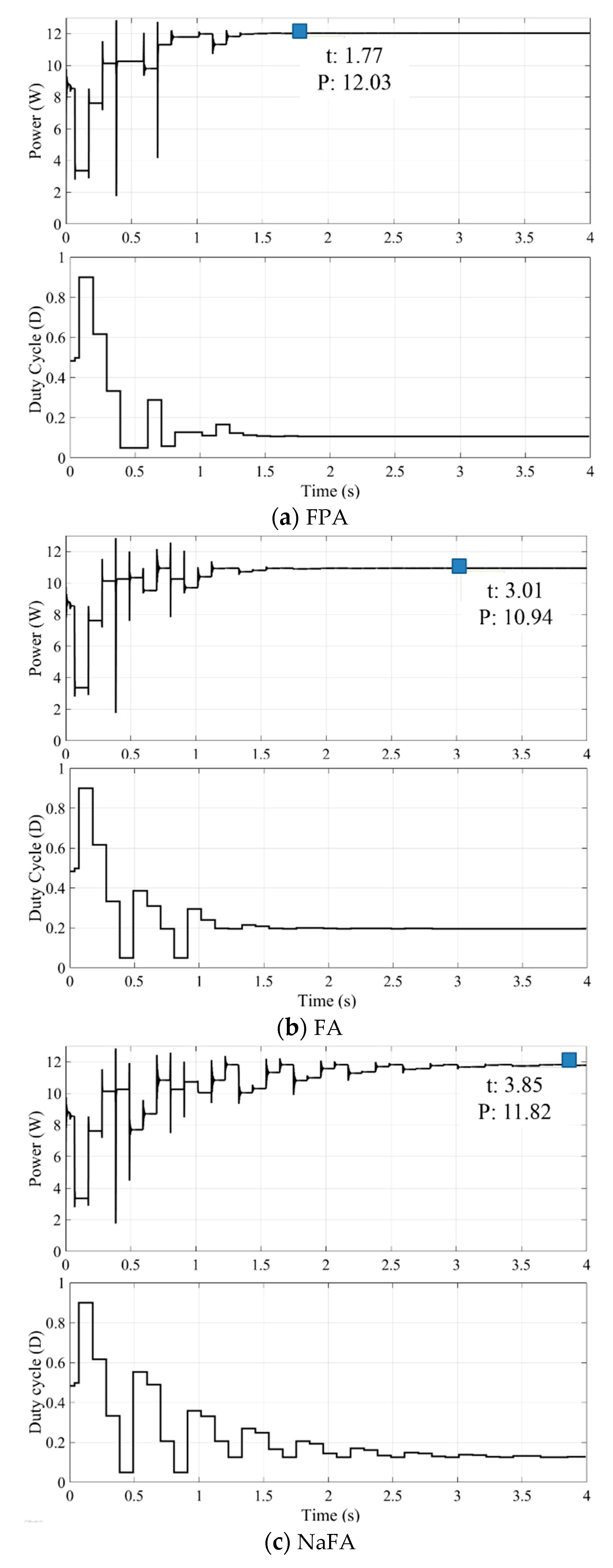
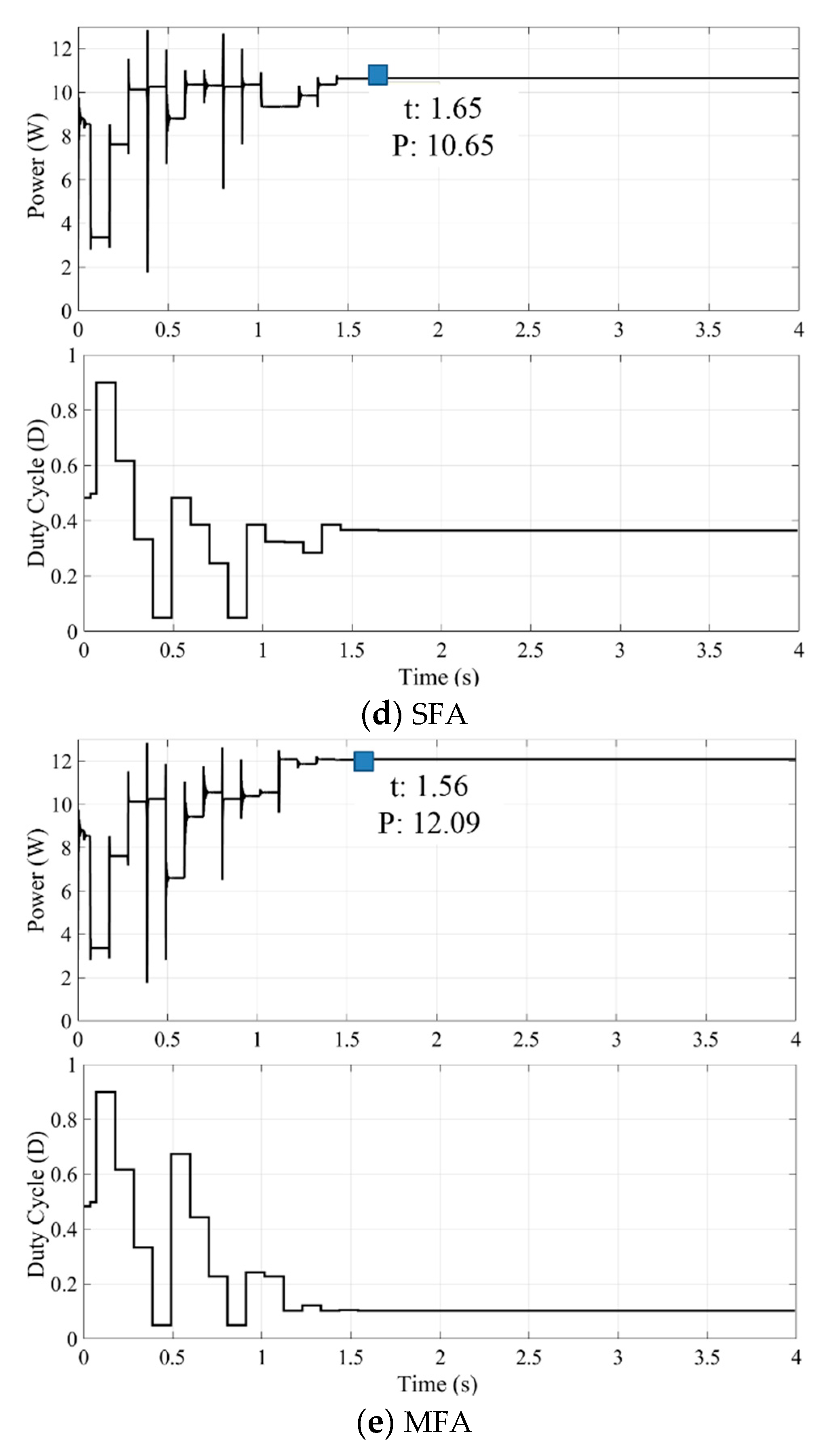
Figure 13 and Figure 14 illustrate the variations in the output power and corresponding duty cycle during the simulated tracking processes of the five algorithms under PSC Pattern #4 and Pattern #10, respectively. The t and P that are marked in the figures represent execution time of the algorithm and power of its estimated MPP, respectively. It is observed in Figure 13 that under Pattern #4, which exhibits three LMPPs, the MFA has the shortest execution time and good power output. Although the FPA and FA have larger power output, the execution time is longer. On the other hand, it is observed that the NaFA could not satisfy the convergence criteria by the end of this period. Figure 14 illustrates that under Pattern #10, which exhibits four LMPPs, the FPA and MFA have the shortest execution times and largest output power during the process. Comparatively, the FA and NaFA have longer execution times, while the FA and SFA have lower power output, respectively.

Table 10. Comparison of the simulation results of the five algorithms at 25 °C.

Algorithms	Averaged Sampling Times	Averaged Time (ms)	Averaged Error (%)	Averaged Efficiency (%)
FPA	22.90	19.57	2.30	93.62
FA	24.54	16.45	2.73	92.95
NaFA	53.01	34.74	3.19	91.5
SFA	14	9.95	5.29	92.34
MFA	13.16	13.20	1.25	95.37

summarizes the simulation results. Here, sampling times, execution times, tracking errors and efficiencies for the five algorithms under the PSC 10 patterns are averaged and compared. Under the simulation conditions, the MFA has the fewest sampling times, smallest error and highest efficiency. When compared with the other algorithms, the averaged sampling times of the MFA could be reduced around 0.84 (6.00%) to 39.85 (75.17%) during the tracking process. In addition, although the averaged execution time of the MFA is longer than the SFA by approximately 3.25 ms, it is around 6.37, 3.25, and 21.54 ms shorter when compared with the FPA, FA, and NaFA, respectively. Furthermore, when compared with the FPA, FA, NaFA, and SFA, the averaged error of the MFA is around 1.05%, 1.48%, 1.94%, and 4.04% lower, respectively, under the simulation conditions. In addition, when compared with the FPA, FA, NaFA, and SFA, the averaged efficiency of the MFA is around 1.75%, 2.42%, 3.87%, and 3.03% higher, respectively.

To evaluate the temperature effect, the simulation was again conducted at NOCT. Specifications of the PV array, irradiation patterns, parameters setting of the algorithms, and convergence criteria were all the same as those described in the Simulation setup section. In addition, performance of the proposed MFA algorithm was tested at five different cell temperatures (25 °C, 35 °C, 45 °C, 55 °C, and 65 °C).

Table 11. Simulation results comparison of the five algorithms at 45 °C.

Algorithms	Averaged Sampling Times	Averaged Time (ms)	Averaged Error (%)	Averaged Efficiency (%)
FPA	22.63	19.34	6.75	87.75
FA	24.13	16.18	5.65	89.56
NaFA	45.17	29.6	2.38	90.91
SFA	13.18	9.38	6.42	90.2
MFA	13.1	13.14	3.09	93.52

summarizes the simulation results of the five algorithms at NOCT (45 °C), in which sampling times, execution times, tracking errors, and efficiencies for the five algorithms under the 10 PSC patterns are averaged and compared. When compared with Table 10, it can be observed that the averaged sampling times, execution time and error of the NaFA are lower at 45 °C, which might be due to V_OC decreasing with temperature. For the other four algorithms, the averaged sampling times and execution time are roughly the same at 25 °C and 45 °C. However, the averaged error increased and averaged efficiency decreased for all five algorithms at higher temperature.

Table 12. Performance of the proposed MFA at different temperature.

Temperature	Averaged Sampling Times	Averaged Time (ms)	Averaged Error (%)	Averaged Efficiency (%)
25	13.16	13.20	1.25	95.37
35	13.08	13.04	2.29	94.61
45	13.1	13.14	3.09	93.52
55	13.28	13.24	2.43	93.67
65	13.11	13.07	2.32	93.07

lists the performance comparison of the proposed MFA at five different temperatures. As shown, it appears that the averaged sampling times and execution time are unaffected by cell temperature. However, it is observed that, when compared with 25 °C, the averaged error of the proposed MFA, respectively, increased around 1.04%, 1.84%, 1.18%, and 1.07% as the temperature increased from 35 to 65 °C. Similarly, when compared with 25 °C, the averaged efficiency of the MFA, respectively, decreased around 0.76%, 1.85%, 1.7%, and 2.3 % as the temperature increased from 35 to 65 °C.

4. System Evaluation

4.1. Evaluation System Setup

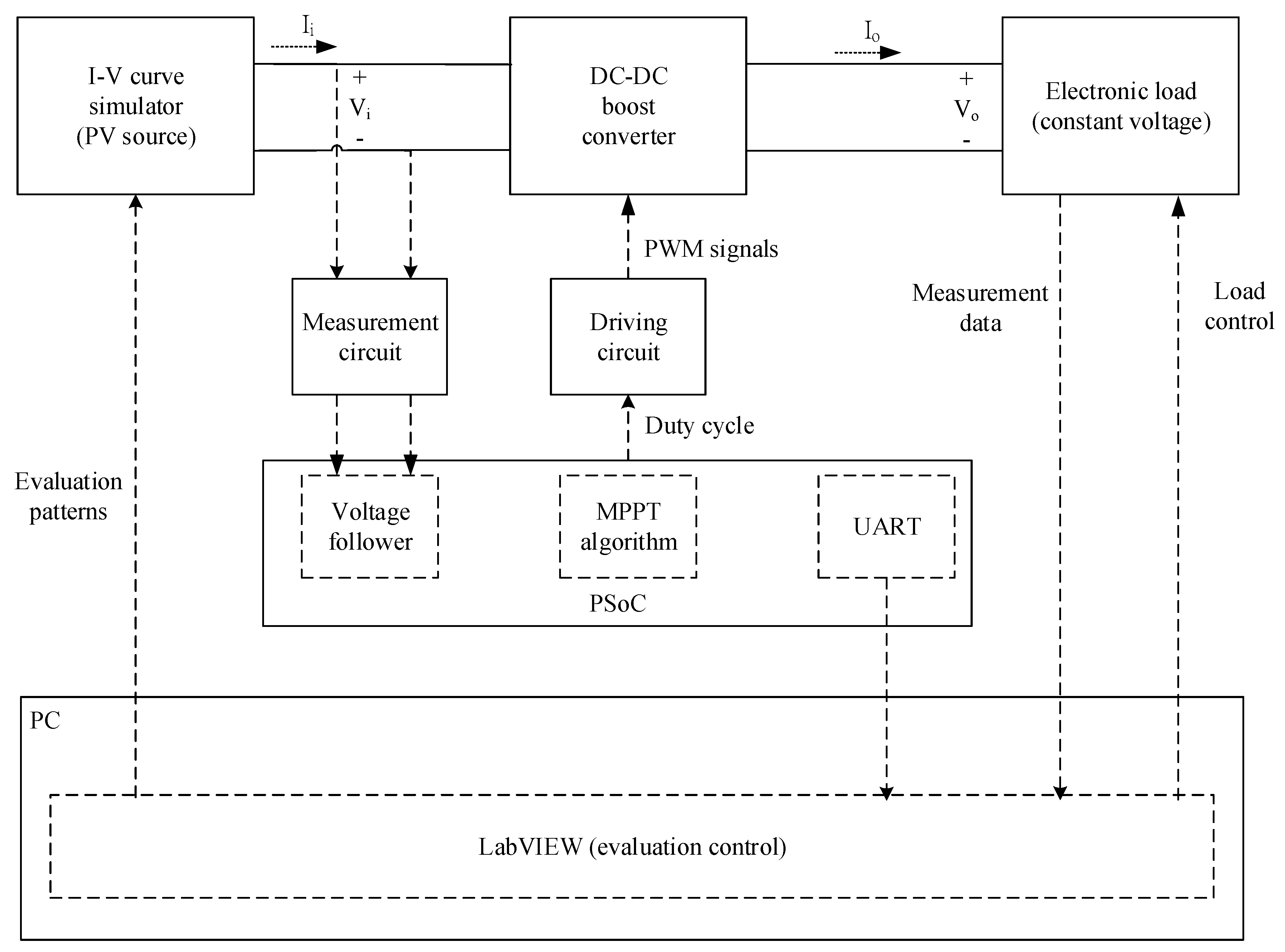
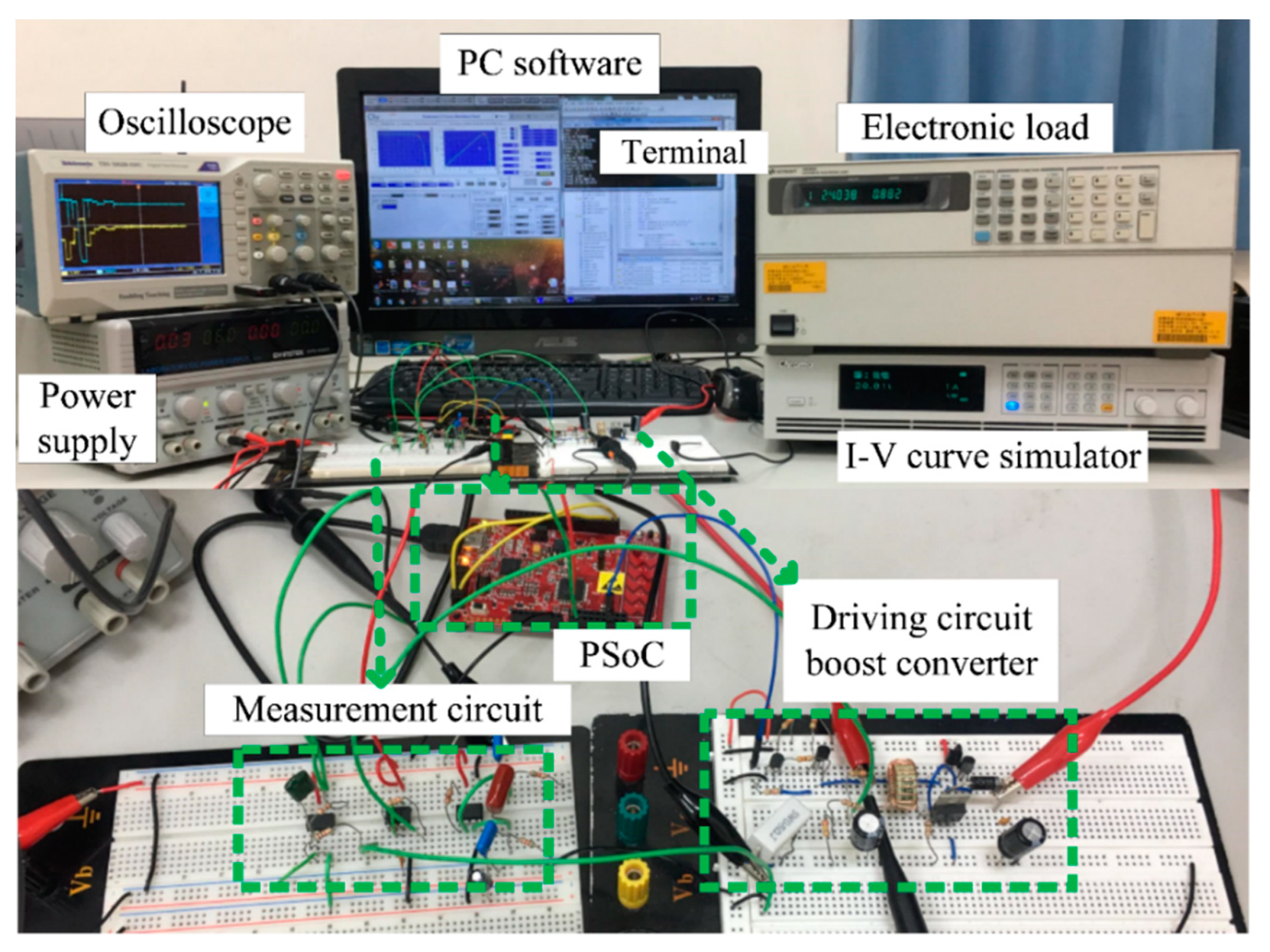
To further verify the MPP tracking speed and tracking accuracy of the proposed MFA, a hardware evaluation system was installed, the structure and signal flow of which is illustrated in Figure 15. An I-V curve simulator (Chroma, 62020H) was utilized to simulate the PV array output under different PSCs. Specifications of the PV array and the 10 irradiation patterns were the same as described in the Simulation setup section. A DC-DC boost converter controlled by a PWM signal was used as the interface to feed the output power of the PV array to a programmable electronic load (Keysight, N3300A) that is set at constant voltage mode. The specifications of the boost converter are listed in

Table 13. Specifications of the boost converter.

Parameter	Value
Switching frequency	100 kHz
Inductor	35 μH
Capacitor	35 V, 470 μF
Electronic load	Constant voltage

. The five MPPT algorithms, namely the FPA, FA, NaFA, SFA, and the proposed MFA, were coded and executed using a programmable system-on-chip controller (Cypress, PSoC), which has an ARM Cortex-M0 core running at 48 MHz. The operating point of the PV array’s I-V curve was controlled by adjusting the duty cycle of the PWM signal. Meanwhile, the input voltage V_i and current I_i of the boost converter were measured with the measurement circuit, the PSoC’s onboard programmable amplifier circuit and the analog-to-digital (A/D) converters. All of the evaluation experiments were conducted and controlled by a PC software programmed in LabVIEW (National Instruments). Figure 16 presents a photograph of the evaluation system.

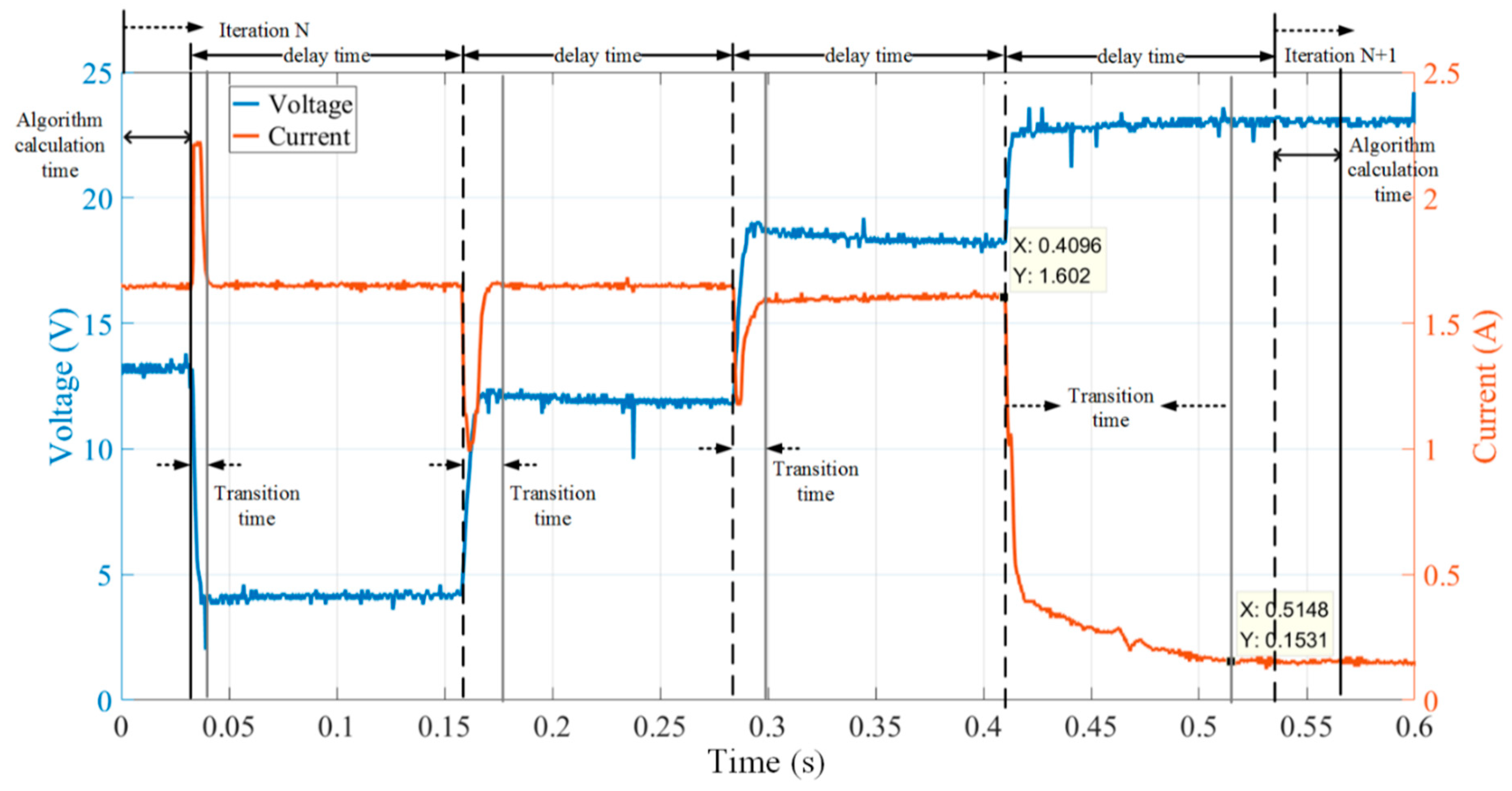
Since the I_SC of the simulated PV array is around 1.43 A, the maximum transition time needed for the converter and load to reach stead state was approximately 105 ms. Consequently, a 200 ms delay time was set to ensure a stable output for each operating point adjustment. Figure 17 illustrates the voltage and current variations of the PV array being controlled by the proposed MFA. At the onset of each iteration, the calculations of the algorithm were processed; then, four operating points were sequentially executed with the 200 ms delay time for each transition to reach its steady state for measurement.

4.2. Evaluation Results

Evaluation experiments were conducted 100 times under the same simulation conditions.

Table 14. Evaluation results of the tracking speed, accuracy and efficiency.

Patterns	Algorithms	Time (s)	Voltage (volts)	Current (amperes)	Power (watts)	GMPP (watts)	Error (%)	Efficiency (%)
Pattern #1	FPA	4.742	19.079	1.483	28.284	28.620	1.174	85.87
	FA	4.162	18.926	1.489	28.182		1.530	91.31
	NaFA	10.46	19.649	1.454	28.566		0.009	89.58
	SFA	3.3268	18.930	1.489	28.185		1.519	90.72
	MFA	3.12	19.883	1.436	28.550		0.244	91.38
Pattern #2	FPA	5.014	15.004	1.427	21.408	21.486	0.364	86.00
	FA	4.216	15.072	1.418	21.371		0.534	92.06
	NaFA	10.42	15.064	1.417	21.346		0.652	87.98
	SFA	3.341	14.827	1.448	21.473		0.059	91.11
	MFA	3.701	15.333	1.3795	21.152		1.555	89.05
Pattern #3	FPA	4.755	17.944	0.843	15.120	16.107	6.131	81.62
	FA	4.365	17.859	0.843	15.052		6.548	86.34
	NaFA	10.54	19.250	0.833	16.037		0.432	84.14
	SFA	3.31	17.899	0.843	15.088		6.329	87.18
	MFA	3.301	18.899	0.840	15.883		1.389	90.57
Pattern #4	FPA	4.168	5.139	1.357	6.975	7.090	1.622	76.72
	FA	9.16	5.145	1.355	6.973		1.655	68.21
	NaFA	27.42	5.443	0.984	5.357		24.44	53.97
	SFA	4.4	5.208	1.318	6.866		3.162	76.79
	MFA	5.384	5.130	1.363	6.994		1.363	80.35
Pattern #5	FPA	5.316	19.010	0.843	16.031	16.780	4.461	81.27
	FA	4.196	15.063	1.103	16.609		1.020	92.01
	NaFA	27.31	15.753	1.049	16.518		1.502	83.41
	SFA	3.48	14.353	1.168	16.767		0.075	92.73
	MFA	4.84	15.074	1.099	16.572		1.239	90.59
Pattern #6	FPA	10.37	18.645	0.986	18.374	19.610	6.300	72.34
	FA	4.472	18.087	0.986	17.834		9.056	84.66
	NaFA	17.18	19.295	0.981	18.930		3.465	83.76
	SFA	3.21	18.015	0.845	15.224		22.3638	72.14
	MFA	3.248	19.148	0.984	18.838		3.938	87.89
Pattern #7	FPA	4.164	5.096	1.376	7.011	7.179	2.335	78.35
	FA	9.641	5.147	1.347	6.932		3.429	71.58
	NaFA	27.42	5.380	1.085	5.836		18.70	58.94
	SFA	4.148	5.297	1.225	6.487		9.630	73.01
	MFA	5.384	5.114	1.366	6.984		2.707	75.19
Pattern #8	FPA	5.02	14.629	0.663	9.697	10.830	10.457	80.33
	FA	3.89	14.755	0.657	9.691		10.519	83.54
	NaFA	27.52	9.5133	1.113	10.592		2.188	81.16
	SFA	4.16	10.248	1.024	10.489		3.1502	87.67
	MFA	3.96	9.846	1.099	10.823		0.063	88.54
Pattern #9	FPA	6.172	14.705	0.839	12.331	12.339	0.063	85.78
	FA	4.208	14.933	0.826	12.339		0.002	92.45
	NaFA	12.81	14.629	0.838	12.263		0.636	85.56
	SFA	4.164	10.315	1.071	11.047		10.471	82.37
	MFA	4.42	14.417	0.843	12.148		1.549	87.34
Pattern #10	FPA	5.024	17.693	0.685	12.112	12.701	4.632	83.73
	FA	5.028	17.615	0.686	12.086		4.842	89.2
	NaFA	13.67	18.528	0.676	12.527		1.369	83.28
	SFA	3.326	17.608	0.686	12.079		4.897	88.54
	MFA	3.124	18.647	0.677	12.622		0.618	90.22

summarizes the evaluation results of the execution times, estimated MPPs, errors, and efficiencies of the five MPPT algorithms under the 10 PSCs. The voltage, current, and power of each MPPT algorithm’s estimated MPP were averaged and compared. Estimated MPPs with abnormal operating voltage and lower power might indicate that the MPPT was trapped at one of the LMPPs. For instance, the FPA became trapped under Patterns #5 and #8; the FA became trapped under Pattern #8; and, the SFA became trapped under Pattern #9. Comparatively, the NaFA and MFA did not become trapped at any of the LMPPs. In addition, time is defined as the total execution time needed for the tracking processes to reach convergence. Furthermore, error and efficiency are defined as previously stated in the Simulation setup section. It is observed that the MFA was the only algorithm with an average error smaller than 4% under all the patterns. In addition, under Patterns #1, #3, #6, #8, and #10, the NaFA and MFA had smaller errors than the other algorithms. However, the execution times of the NaFA were larger than the other algorithms under all patterns. Moreover, the execution times of the NaFA under Patterns #4, #5, #7, and #8 were exceedingly long, which might be due to it not being able to satisfy the convergence criteria by the end of the evaluation period. Furthermore, under Patterns #1, #3, #4, #6, #8, and #10, the MFA had the highest efficiency among the tested algorithms. In contrast, the efficiency of the NaFA was the lowest of the tested algorithms under Patterns #4, #7, and #10. Accordingly, the proposed MFA holds strong potential, as it offered rapid response time with high accuracy and efficiency under all evaluation conditions.

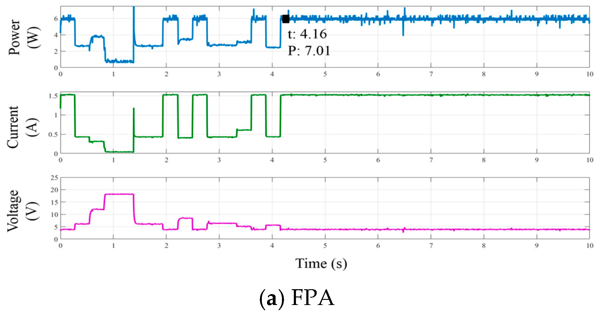
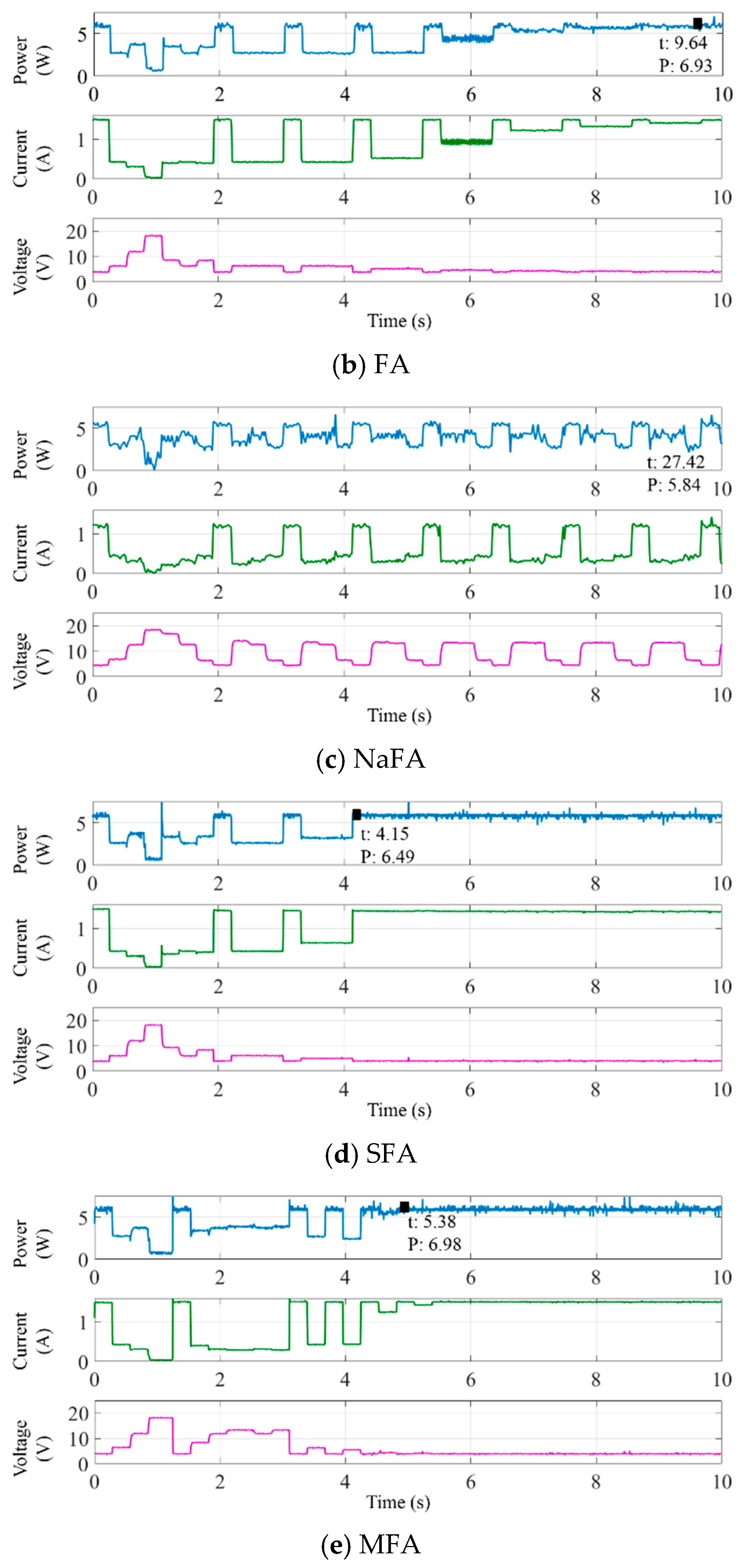
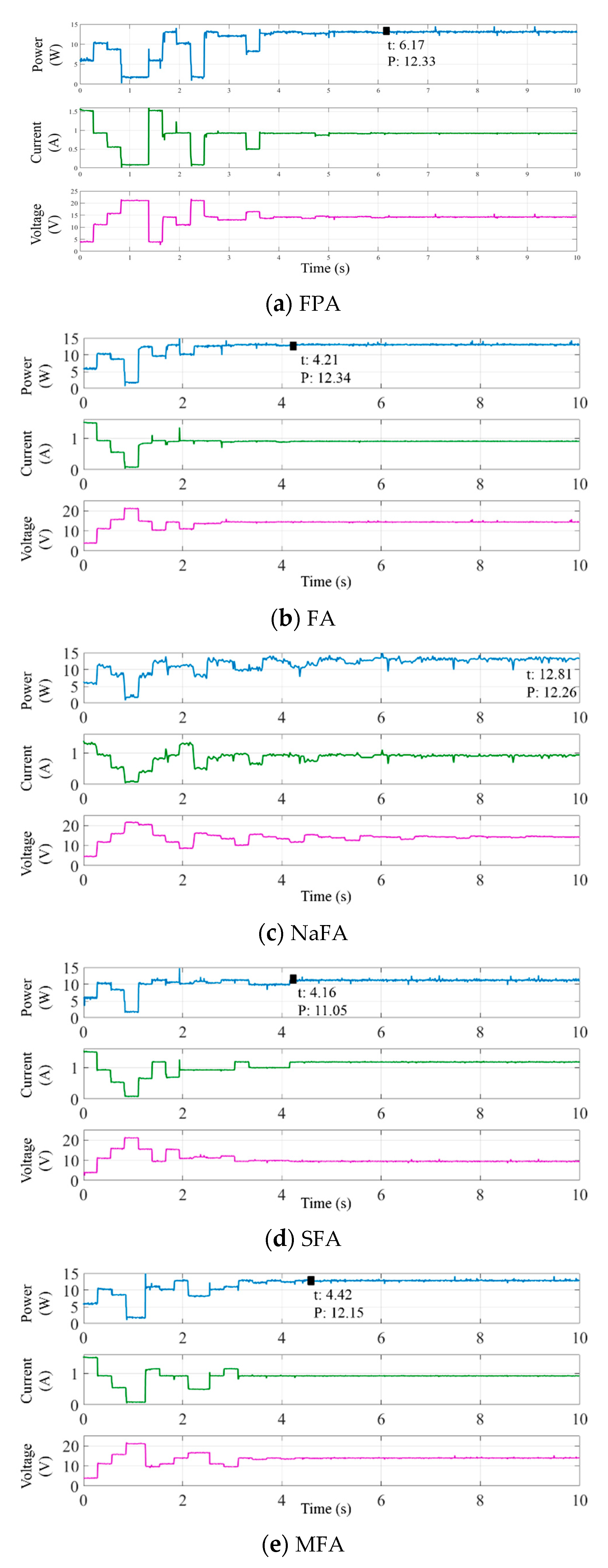
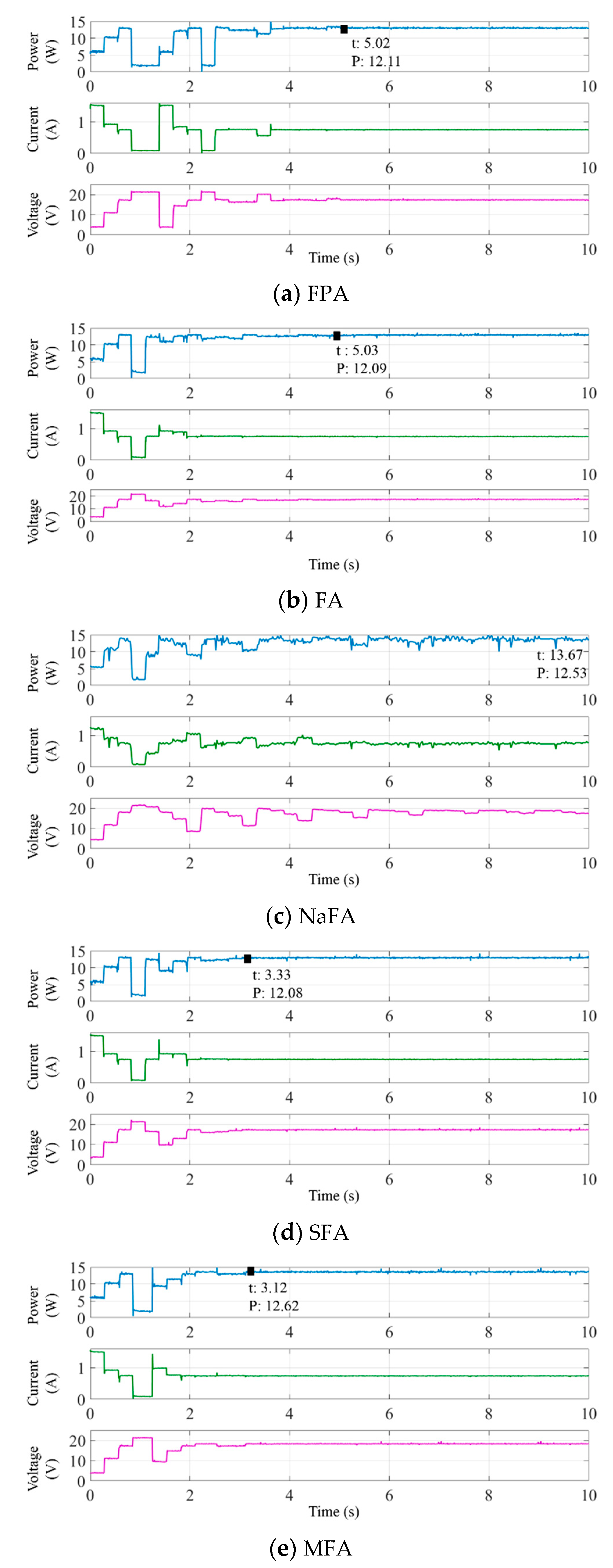
Figure 18, Figure 19 and Figure 20 illustrate the variations in the power, current, and voltage during one evaluation tracking process of the five algorithms under Patterns #7, #9, and #10, respectively. The three chosen patterns all exhibit four intervals and four LMPPs in the P-V curve, the difference being that the location of their GMPPs are in the leftmost, middle, and rightmost intervals, respectively. The t and P marked in the figures represent the execution time of the algorithm and power of its estimated MPP, respectively. It is observed that when the location of the GMPP is in the leftmost interval and close to I_SC, as with Pattern #7, the execution times of the FPA, SFA, and MFA are shorter than those of the other two algorithms. In addition, under this condition, the estimated MPP power of the FPA, FA, and MFA are larger than those of the others two. When the location of the GMPP is in the middle 2 intervals of the P-V curve, as with Pattern #9, the FA and MFA have shorter execution times and larger power output. Moreover, when the location of the GMPP is in the rightmost interval and close to V_OC, as with Pattern #10, the execution times of the FA, SFA, and MFA are shorter, while the FPA, NaFA, and MFA have larger output power. Evaluations of the other patterns, which have two or three LMPPs exhibit similar results. Consequently, the proposed MFA can provide both shorter execution time and larger output power when the location of the GMPP moves.

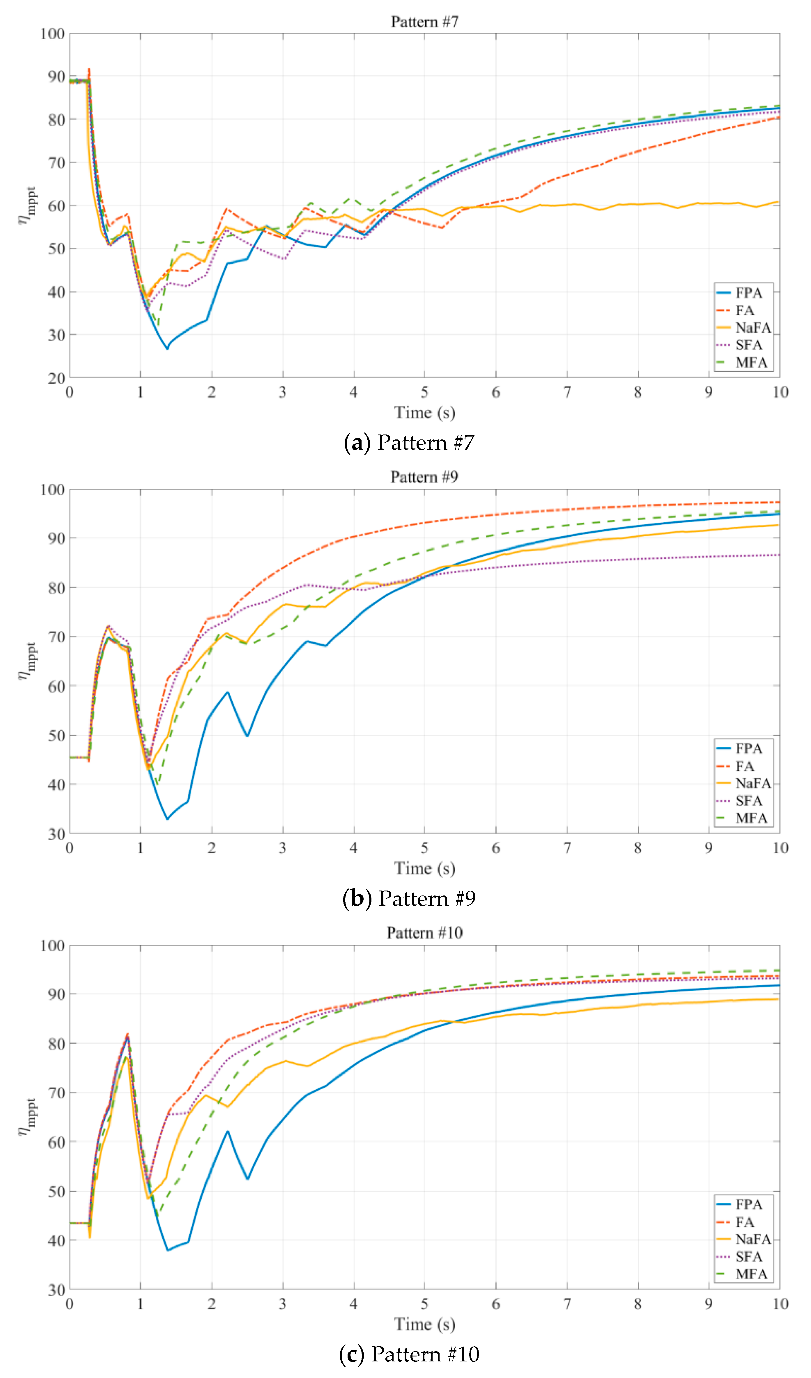
Figure 21 illustrates the variations in efficiency during one evaluation tracking process of the five algorithms under Patterns #7, #9, and #10, respectively. It can be seen that the efficiencies of all five algorithms exhibit large damping and deviation during the initial iterations. Nevertheless, the efficiency curves of the proposed MFA quickly become stable, especially after the convergence judgment criteria are satisfied. In addition, although all five algorithms have relatively lower efficiencies under Pattern #7, the proposed MFA has the best efficiency under Patterns #7 and #10. Furthermore, the FA and MFA have the highest efficiencies under Pattern #9.

Table 15. Comparison of the evaluation results of the five algorithms.

Algorithms	Averaged Execution Time (s)	Averaged Error (%)	Averaged Efficiency (%)
FPA	5.48	3.74	81.201
FA	5.33	3.90	85.136
NaFA	18.47	5.35	79.178
SFA	3.69	6.15	84.226
MFA	4.05	1.45	87.112

summarizes the evaluation results of the five algorithms under the 10 PSC patterns. Here, the execution times, tracking errors and efficiencies are averaged and compared. Under the evaluation conditions, the MFA has the lowest error and highest efficiency. When compared with the FPA, FA, NaFA, and SFA, the averaged error of the MFA can be, respectively, improved around 2.29%, 2.45%, 3.90%, and 4.70%; in addition, the averaged efficiency of the MFA was higher by around 5.91%, 1.98%, 7.93%, and 2.89%, respectively. Although the averaged execution time of the MFA is longer than that of the SFA by around 0.36 s (9.8%), it is shorter by approximately 1.43 s (26.09%), 1.28 s (24.02%), and 14.42 s (78.07%) when compared with the FPA, FA, and NaFA, respectively.

5. Discussion and Conclusions

Although the conventional FA can accurately extract the GMPP under PSCs, the tracking speed can be further improved. In addition, despite the convergence process being simplified, accuracy tended to decline with decreasing processing time. Furthermore, simplified calculation processes might cause the search results to become trapped at LMPPs. In response, this work proposed a fusion algorithm that integrates the NaFA and SFA for MPPT. A modified attraction process for the NaFA was used in the first iteration to avoid trapping at LMPPs. The attractiveness factor of the attraction process was specifically designed to relate to the power and location difference of the fireflies, which improved its processing speed. For the second and following iterations, a modified SFA with convergence-speed-improved processes was implemented. The number of fireflies was designed to decrease in proportion with the iterations, which improved the convergence speed. To our knowledge, this is the first study that evaluated the fusion of the NaFA and SFA for photovoltaic MPPT.

Although integrating the NaFA and SFA leads to an execution time that is slightly longer than the original SFA, the simulation and evaluation results demonstrate that the proposed algorithm offers shorter execution times, smaller error and higher efficiency when encountering PSCs. In addition, it can avoid becoming trapped at LMPPs and ease oscillations during the search process. For instance, the evaluation results demonstrate that, when compared to the FPA, FA, NaFA, and SFA algorithms, the tracking error of the proposed algorithm can be, respectively, improved around 2.29%, 2.45%, 3.90%, and 4.70%; in addition, the averaged efficiency of the MFA was higher by around 5.91%, 1.98%, 7.93%, and 2.89%, respectively. In addition, although the averaged execution time of the MFA is longer than the SFA by 9.8%, it is 26.09%, 24.02%, and 78.07% faster when compared with the FPA, FA, and NaFA, respectively.

Table 16. Qualitative comparison of the proposed method with other algorithms.

No.	Parameters	P&O	ABC	Cuckoo	FPA	FA	NaFA	SFA	MFA
1	Tracking speed	Slow	Fast	Fast	Moderate	Moderate	Slow	Fast	Fast
2	Tracking accuracy	Low	Moderate	High	High	High	Moderate	Moderate	High
3	Trapping at LMPPs	High	Low	Low	Low	Low	Low	Moderate	Low
4	Steady state oscillation	Large	Zero	Zero	Zero	Zero	Zero	Zero	Zero
5	Complexity	Low	High	Moderate	Moderate	Low	Low	Low	Moderate
6	Execution time	Slow	Moderate	Moderate	Moderate	Moderate	Slow	Fast	Fast
7	Efficiency	Moderate	Moderate	High	Moderate	High	Low	High	High

presents a qualitative comparison of the proposed method with other algorithms, namely the P&O, ABC, Cuckoo, FPA, FA, NaFA, and SFA. The performance evaluation of the MPPT techniques are qualitatively weighed using: (1) tracking speed; (2) tracking accuracy; (3) trapping at LMPPs; (4) steady state oscillation; (5) complexity; (6) execution time; and, (7) efficiency. In addition, the parameters are gauged qualitatively as ‘fast/high’, ‘moderate’, and ‘slow/low’. As can be seen, although the fusion process slightly increases the complexity of the proposed method, it offers rapid tracking speed with high accuracy and efficiency. In addition, the proposed method is adaptable to different types of solar panels and different system formats with specifically designed parameters.

Since the experimental PV array was composed of four series-connected modules, the maximum number of LMPPs for the array’s P-V curve under PSCs was four. From the simulation results of this study, the optimized population number of the evaluated algorithms was the same as the number of LMPPs. Future studies could investigate the relationship between the module number of the array and the population number of the proposed algorithm, and further expand the prototype to larger scale arrays. Furthermore, the control range of the PWM’s duty cycle is around 0.1 to 0.85; as such, future studies could also further improve this range by optimizing the performance of the converter.

References

- Eltawil, M.A.; Zhao, Z. Mppt techniques for photovoltaic applications. Renew. Sustain. Energy Rev. 2013, 25, 793–813. [Google Scholar] [CrossRef]
- Femia, N.; Petrone, G.; Spagnuolo, G.; Vitelli, M. Optimization of perturb and observe maximum power point tracking method. IEEE Trans. Power Electron. 2005, 20, 963–973. [Google Scholar] [CrossRef] [Green Version]
- Xuesong, Z.; Daichun, S.; Youjie, M.; Deshu, C. The simulation and design for mppt of pv system based on incremental conductance method. In Proceedings of the 2010 WASE International Conference on Information Engineering, Beidaihe, China, 14–15 August 2010; pp. 314–317. [Google Scholar]
- Dileep, G.; Singh, S.N. Application of soft computing techniques for maximum power point tracking of spv system. Sol. Energy 2017, 141, 182–202. [Google Scholar] [CrossRef]
- Belhachat, F.; Larbes, C. A review of global maximum power point tracking techniques of photovoltaic system under partial shading conditions. Renew. Sustain. Energy Rev. 2018, 92, 513–553. [Google Scholar] [CrossRef]
- Li, G.; Jin, Y.; Akram, M.W.; Chen, X.; Ji, J. Application of bio-inspired algorithms in maximum power point tracking for pv systems under partial shading conditions—A review. Renew. Sustain. Energy Rev. 2018, 81, 840–873. [Google Scholar] [CrossRef]
- Huang, Y.-P.; Chen, X.; Ye, C.-E. A hybrid maximum power point tracking approach for photovoltaic systems under partial shading conditions using a modified genetic algorithm and the firefly algorithm. Int. J. Photoenergy 2018, 2018, 7598653. [Google Scholar] [CrossRef]
- Danandeh, M.A.; Mousavi, G.S.M. Comparative and comprehensive review of maximum power point tracking methods for pv cells. Renew. Sustain. Energy Rev. 2018, 82, 2743–2767. [Google Scholar] [CrossRef]
- Liu, L.; Meng, X.; Liu, C. A review of maximum power point tracking methods of pv power system at uniform and partial shading. Renew. Sustain. Energy Rev. 2016, 53, 1500–1507. [Google Scholar] [CrossRef]
- Prasanth Ram, J.; Rajasekar, N. A new global maximum power point tracking technique for solar photovoltaic (pv) system under partial shading conditions (psc). Energy 2017, 118, 512–525. [Google Scholar] [CrossRef]
- Ram, J.P.; Rajasekar, N. A novel flower pollination based global maximum power point method for solar maximum power point tracking. IEEE Trans. Power Electron. 2017, 32, 8486–8499. [Google Scholar]
- Yang, X.-S. Chapter 8—Firefly algorithms. In Nature-Inspired Optimization Algorithms; Elsevier: Oxford, UK, 2014; pp. 111–127. [Google Scholar]
- Sundareswaran, K.; Peddapati, S.; Palani, S. Mppt of pv systems under partial shaded conditions through a colony of flashing fireflies. IEEE Trans. Energy Convers. 2014, 29, 463–472. [Google Scholar]
- Shi, J.; Zhang, W.; Zhang, Y.; Xue, F.; Yang, T. Mppt for pv systems based on a dormant pso algorithm. Electr. Power Syst. Res. 2015, 123, 100–107. [Google Scholar] [CrossRef]
- Wang, H.; Wang, W.; Zhou, X.; Sun, H.; Zhao, J.; Yu, X.; Cui, Z. Firefly algorithm with neighborhood attraction. Inf. Sci. 2017, 382–383, 374–387. [Google Scholar] [CrossRef]
- Safarudin, Y.M.; Priyadi, A.; Purnomo, M.H.; Pujiantara, M. Maximum power point tracking algorithm for photovoltaic system under partial shaded condition by means updating beta firefly technique. In Proceedings of the 2014 6th International Conference on Information Technology and Electrical Engineering (ICITEE), Yogyakarta, Indonesia, 7–8 October 2014; pp. 1–5. [Google Scholar]
- Mohapatra, A.; Nayak, B.; Das, P.; Mohanty, K.B. A review on mppt techniques of pv system under partial shading condition. Renew. Sustain. Energy Rev. 2017, 80, 854–867. [Google Scholar] [CrossRef]
- Laudani, A.; Riganti Fulginei, F.; Salvini, A. Identification of the one-diode model for photovoltaic modules from datasheet values. Sol. Energy 2014, 108, 432–446. [Google Scholar] [CrossRef]
- Huang, Y.-P.; Hsu, S.-Y. A performance evaluation model of a high concentration photovoltaic module with a fractional open circuit voltage-based maximum power point tracking algorithm. Comput. Electr. Eng. 2016, 51, 331–342. [Google Scholar] [CrossRef]
- Batzelis, E.I.; Routsolias, I.A.; Papathanassiou, S.A. An explicit pv string model based on the lambert w function and simplified mpp expressions for operation under partial shading. IEEE Trans. Sustain. Energy 2014, 5, 301–312. [Google Scholar] [CrossRef]
- Safarudin, Y.M.; Priyadi, A.; Purnomo, M.H.; Pujiantara, M. Combining simplified firefly and modified p&o algorithm for maximum power point tracking of photovoltaic system under partial shading condition. In Proceedings of the 2015 International Seminar on Intelligent Technology and Its Applications (ISITIA), Surabaya, Indonesia, 20–21 May 2015; pp. 181–186. [Google Scholar]
Figure 1.
Solar cell model.
Figure 2.
A photovoltaic (PV) string with m modules connected in series and protected by the bypass and blocking diodes.
Figure 3.
Operation of a PV array under (a) uniform irradiance and (b) partial shading conditions (PSCs).
Figure 4.
(a) I-V and (b) power-voltage (P-V) curves of the PV array under uniform irradiance and PSCs.
Figure 5.
Adjustment of operating points along the P-V curve of a PV array under PSCs with the simplified firefly algorithm (SFA).
Figure 6.
Adjustment of operating points along the P-V curve of a PV array under PSCs with the firefly algorithm with neighborhood attraction (NaFA).
Figure 7.
Processing flow of the modified firefly algorithm (MFA).
Figure 8.
Relationship between the movement step size, distance Dij, and initial attractiveness β0 in the attraction process.
Figure 9.
Relationship between step size, distance Dij and power difference ratio PDRij of the proposed NaFA process.
Figure 10.
Relationship between the step sizes, degree of attractiveness βSFA and distance Dij in the SFA process.
Figure 11.
System blocks for simulation.
Figure 12.
P-V curves of the 10 PSC patterns in the simulation.
Figure 13.
Power and duty cycle variations during one simulated tracking process for the five algorithms under PSC Pattern #4.
Figure 14.
Power and duty cycle variations during one simulated tracking process for the five algorithms under PSC Pattern #10.
Figure 15.
Evaluation system structure.
Figure 16.
Photograph of the evaluation system.
Figure 17.
Operating point adjustment and delay time setting of the proposed MFA.
Figure 18.
Power, current, and voltage variations during one evaluation tracking process of the five algorithms under Pattern #7.
Figure 19.
Power, current, and voltage variations during one evaluation tracking process of the five algorithms under Pattern #9.
Figure 20.
Power, current and voltage variations during one evaluation tracking process of the five algorithms under Pattern #10.
Figure 21.
Efficiency variations during one evaluation tracking process of the five algorithms under Patterns #7, #9, and #10.